Embed Size (px)
Citation preview
1 Exam 1 Spring 2020 AERE 331 Take-Home Due 2/14(F) SOLUTION [NOTE: All work, answers and plots must be placed directly beneath the given problem part to receive credit. Matlab code that supports the same
should be placed in the Appendix. I will not go to the Appendix to search for answers and concepts used to obtain them.]
PROBLEM 1(30pts) In the absence of feedback control, the velocity/thrust transfer function for a satellite in deep space
is given by: ssGv 10/1)( .
(a)(5pts) Assuming the thruster can actually generate an impulse, f(t)=100δ(t), for this input, arrive at the expression for
)(tv .
Solution: ( ) 100F s . And so: ( ) ( ) ( ) 10 /vV s G s F s s . Hence, )(110)( ttv .
(b)(5pts) Explain why, in reality, the craft cannot behave in the manner associated with your answer in (a) using the
concept F=ma.
Explanation: From (a): ( ) 101( ) ( ) 10 ( )v t t a t t , which states that the acceleration at 0t is infinite.
[NOTE: Nonetheless, this can be a useful model, depending on the time scale and/or bandwidth of interest.]
(c)(10pts) It should be clear that the satellite position/thrust transfer function is: 210/1)( ssGp . Design a PD controller
so that the unity feedback CL position system will have critical damping ( 1 ) and sec2 . To this end, use the
method of equating coefficients associated with the CL characteristic polynomial. Do not use the root locus method.
Solution:
For PDc KsKsG )( , the OLTF is
210)()()(
s
KsKsGsGsG PD
pc
& the CLTF is
PD
PD
KsKs
KsKsW
210)( .
5.0/1284 . Hence, 25.0)5.0(1.01.0)( 222 sssKsKssp PD.
Equating coefficients gives: PK 2.5 and
DK 10 . Hence: ( )cG s s 10 2.5 .
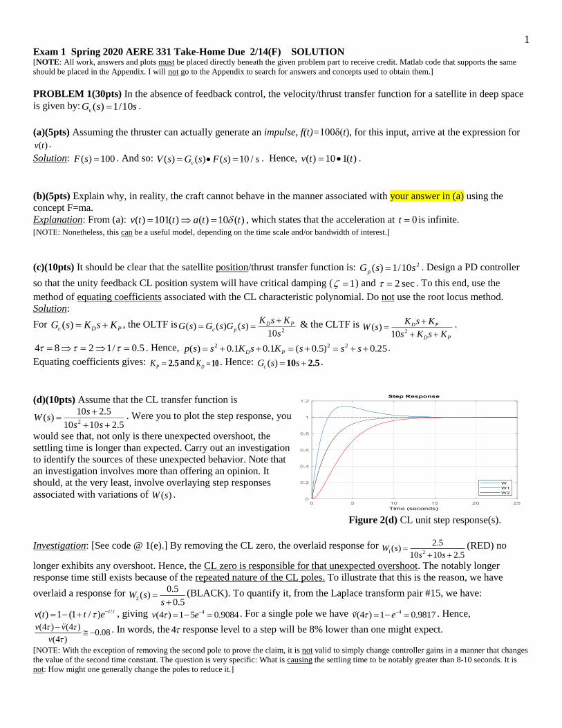
(d)(10pts) Assume that the CL transfer function is
5.21010
5.210)(
2
ss
ssW . Were you to plot the step response, you
would see that, not only is there unexpected overshoot, the
settling time is longer than expected. Carry out an investigation
to identify the sources of these unexpected behavior. Note that
an investigation involves more than offering an opinion. It
should, at the very least, involve overlaying step responses
associated with variations of ( )W s .
Figure 2(d) CL unit step response(s).
Investigation: [See code @ 1(e).] By removing the CL zero, the overlaid response for 1 2
2.5( )
10 10 2.5W s
s s
(RED) no
longer exhibits any overshoot. Hence, the CL zero is responsible for that unexpected overshoot. The notably longer
response time still exists because of the repeated nature of the CL poles. To illustrate that this is the reason, we have
overlaid a response for 2
0.5( )
0.5W s
s
(BLACK). To quantify it, from the Laplace transform pair #15, we have:
/( ) 1 (1 / ) tv t t e , giving 4(4 ) 1 5 0.9084v e . For a single pole we have 4(4 ) 1 0.9817v e . Hence,
(4 ) (4 )0.08
(4 )
v v
v
. In words, the 4 response level to a step will be 8% lower than one might expect.
[NOTE: With the exception of removing the second pole to prove the claim, it is not valid to simply change controller gains in a manner that changes
the value of the second time constant. The question is very specific: What is causing the settling time to be notably greater than 8-10 seconds. It is
not: How might one generally change the poles to reduce it.]
2 PROBLEM 2(35pts) A transport aircraft at altitude of 10,000 ft and speed of 487 ft/s has the yaw rate/rudder position
transfer function: 07.013.278.121.2
24.030.043.173.0
)(
)()(
234
23
ssss
sss
s
srsG
r
p
.
(a)(12pts) (i) Compute the plant poles to TWO decimal places. (ii) From these numbers, compute all of the plant time
constants, as well as any damping ratios and damped natural frequencies (again, to TWO decimal places). (iii) Give the
name of the lateral mode associated with each pole (or set of poles).
Solution: [Show ALL work/code HERE.] Rp=roots([1 2.21 1.78 2.13 .07]) = -1.86 ; -0.16 +/- 1.04i ; -0.03
1.86 1/1.86r rp 0.54 s roll mode ; 0.03 1/ 0.03sp spp 33.33 s spiral mode
0.16 1.04 1/ 0.16 ; /dr dr dp i r s 6.25 s 1.04 . th=atan(1.04/.16); ζ=cos(th) =0.15. Dutch roll mode
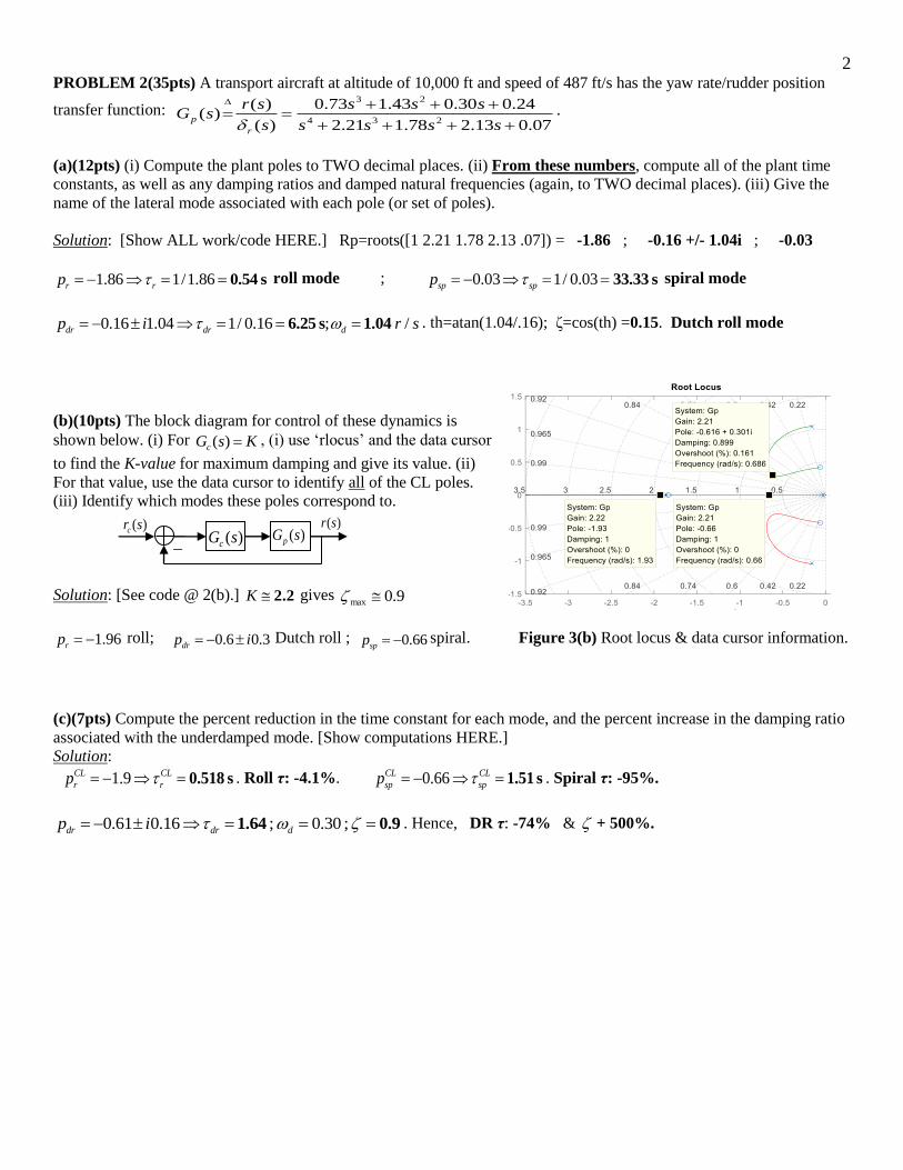
(b)(10pts) The block diagram for control of these dynamics is
shown below. (i) For KsGc )( , (i) use ‘rlocus’ and the data cursor
to find the K-value for maximum damping and give its value. (ii)
For that value, use the data cursor to identify all of the CL poles.
(iii) Identify which modes these poles correspond to.
Solution: [See code @ 2(b).] 2.2K gives 9.0max
1.96rp roll; 0.6 0.3drp i Dutch roll ; 0.66spp spiral. Figure 3(b) Root locus & data cursor information.
(c)(7pts) Compute the percent reduction in the time constant for each mode, and the percent increase in the damping ratio
associated with the underdamped mode. [Show computations HERE.]
Solution:
1.9CL CL
r rp 0.518 s . Roll τ: -4.1%. 0.66CL CL
sp spp 1.51 s . Spiral τ: -95%.
0.61 0.16 ; 0.30 ;dr dr dp i 1.64 0.9 . Hence, DR τ: -74% & + 500%.
)(sGc
)(sr)(src
)(sGp
3
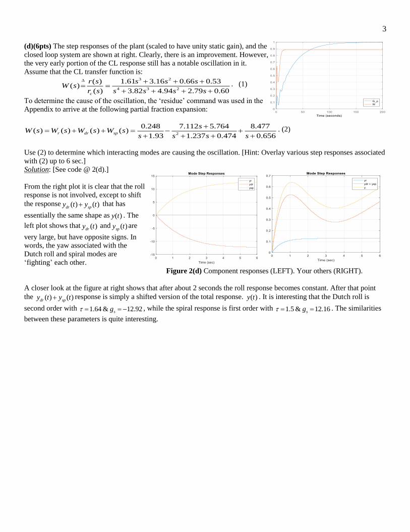
(d)(6pts) The step responses of the plant (scaled to have unity static gain), and the
closed loop system are shown at right. Clearly, there is an improvement. However,
the very early portion of the CL response still has a notable oscillation in it.
Assume that the CL transfer function is:
3 2
4 3 2
( ) 1.61 3.16 0.66 0.53( )
( ) 3.82 4.94 2.79 0.60c
r s s s sW s
r s s s s s
. (1)
To determine the cause of the oscillation, the ‘residue’ command was used in the
Appendix to arrive at the following partial fraction expansion:
2
0.248 7.112 5.764 8.477( ) ( ) ( ) ( )
1.93 1.237 0.474 0.656r dr sp
sW s W s W s W s
s s s s
. (2)
Use (2) to determine which interacting modes are causing the oscillation. [Hint: Overlay various step responses associated
with (2) up to 6 sec.]
Solution: [See code @ 2(d).]
From the right plot it is clear that the roll
response is not involved, except to shift
the response ( ) ( )dr spy t y t that has
essentially the same shape as ( )y t . The
left plot shows that ( )dry t and ( )spy t are
very large, but have opposite signs. In
words, the yaw associated with the
Dutch roll and spiral modes are
‘fighting’ each other.
Figure 2(d) Component responses (LEFT). Your others (RIGHT).
A closer look at the figure at right shows that after about 2 seconds the roll response becomes constant. After that point
the ( ) ( )dr spy t y t response is simply a shifted version of the total response. ( )y t . It is interesting that the Dutch roll is
second order with 1.64 & 12.92sg , while the spiral response is first order with 1.5 & 12.16sg . The similarities
between these parameters is quite interesting.
4
PROBLEM 3(35pts) A motor to be used for a solar array angular positioning has 10( )
( 0.5)pG s
s s
. In this problem you
will design a unity feedback command control system having a pole at 0 2 2s i .
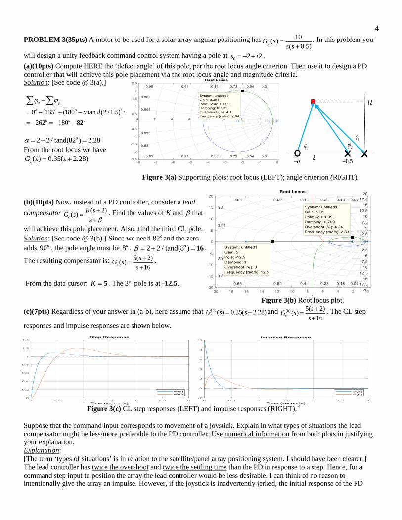
(a)(10pts) Compute HERE the ‘defect angle’ of this pole, per the root locus angle criterion. Then use it to design a PD
controller that will achieve this pole placement via the root locus angle and magnitude criteria.
Solution: [See code @ 3(a).]
0 [135 (180 tan (2 /1.5)]
262 180
z p
o o o
o o
a d
o82
.
2 2 / tand(82 ) 2.28o
From the root locus we have
( ) 0.35( 2.28)cG s s
Figure 3(a) Supporting plots: root locus (LEFT); angle criterion (RIGHT).
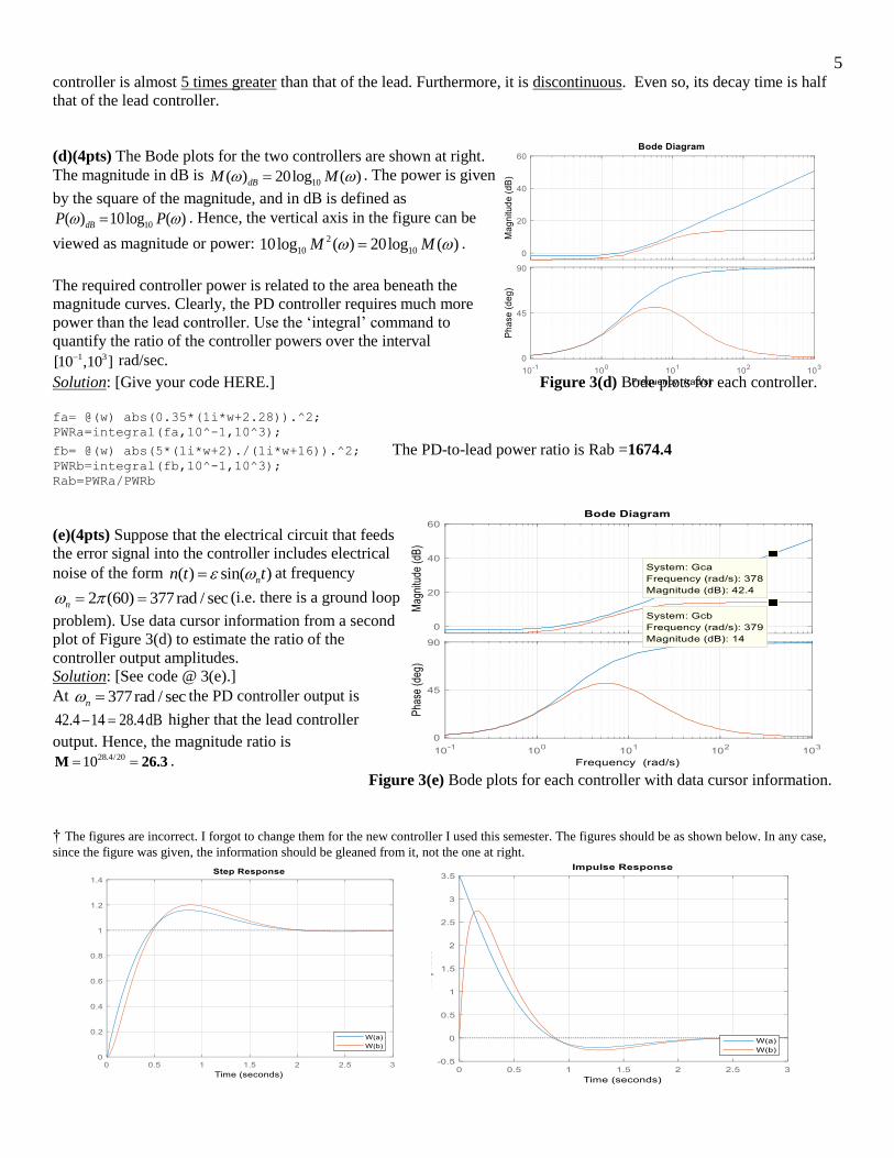
(b)(10pts) Now, instead of a PD controller, consider a lead
compensator ( 2)( )c
K sG s
s
. Find the values of K and that
will achieve this pole placement. Also, find the third CL pole.
Solution: [See code @ 3(b).] Since we need 82o and the zero
adds o90 , the pole angle must be 8o . 2 2 / tand(8 )o 16 .
The resulting compensator is: 5( 2)( )
16c
sG s
s
.
From the data cursor: K 5 . The 3rd pole is at -12.5.
Figure 3(b) Root locus plot.
(c)(7pts) Regardless of your answer in (a-b), here assume that ( ) ( ) 0.35( 2.28)a
cG s s and ( ) 5( 2)( )
16
b
c
sG s
s
. The CL step
responses and impulse responses are shown below.
Figure 3(c) CL step responses (LEFT) and impulse responses (RIGHT). †
Suppose that the command input corresponds to movement of a joystick. Explain in what types of situations the lead
compensator might be less/more preferable to the PD controller. Use numerical information from both plots in justifying
your explanation.
Explanation:
[The term ‘types of situations’ is in relation to the satellite/panel array positioning system. I should have been clearer.]
The lead controller has twice the overshoot and twice the settling time than the PD in response to a step. Hence, for a
command step input to position the array the lead controller would be less desirable. I can think of no reason to
intentionally give the array an impulse. However, if the joystick is inadvertently jerked, the initial response of the PD
2
2i
1
2z
0.5
5 controller is almost 5 times greater than that of the lead. Furthermore, it is discontinuous. Even so, its decay time is half
that of the lead controller.
(d)(4pts) The Bode plots for the two controllers are shown at right.
The magnitude in dB is 10( ) 20log ( )dBM M . The power is given
by the square of the magnitude, and in dB is defined as
10( ) 10log ( )dBP P . Hence, the vertical axis in the figure can be
viewed as magnitude or power: 2
10 1010log ( ) 20log ( )M M .
The required controller power is related to the area beneath the
magnitude curves. Clearly, the PD controller requires much more
power than the lead controller. Use the ‘integral’ command to
quantify the ratio of the controller powers over the interval 1 3[10 ,10 ] rad/sec.
Solution: [Give your code HERE.] Figure 3(d) Bode plots for each controller.
fa= @(w) abs(0.35*(1i*w+2.28)).^2;
PWRa=integral(fa,10^-1,10^3);
fb= @(w) abs(5*(1i*w+2)./(1i*w+16)).^2; The PD-to-lead power ratio is Rab =1674.4 PWRb=integral(fb,10^-1,10^3);
Rab=PWRa/PWRb
(e)(4pts) Suppose that the electrical circuit that feeds
the error signal into the controller includes electrical
noise of the form ( ) sin( )nn t t at frequency
2 (60) 377rad / secn (i.e. there is a ground loop
problem). Use data cursor information from a second
plot of Figure 3(d) to estimate the ratio of the
controller output amplitudes.
Solution: [See code @ 3(e).]
At 377rad / secn the PD controller output is
42.4 14 28.4dB higher that the lead controller
output. Hence, the magnitude ratio is 28.4/2010 M 26.3 .
Figure 3(e) Bode plots for each controller with data cursor information.
† The figures are incorrect. I forgot to change them for the new controller I used this semester. The figures should be as shown below. In any case,
since the figure was given, the information should be gleaned from it, not the one at right.
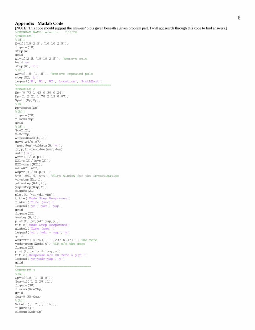
6 Appendix Matlab Code [NOTE: This code should support the answers/ plots given beneath a given problem part. I will not search through this code to find answers.] %PROGRAM NAME: exam1.m 2/3/20
%PROBLEM 1
%(d):
W=tf([10 2.5],[10 10 2.5]);
figure(10)
step(W)
grid
W1=tf(2.5,[10 10 2.5]); %Remove zero
hold on
step(W1,'r')
%(e):
W2=tf(.5,[1 .5]); %Remove repeated pole
step(W2,'k')
legend('W','W1','W2','Location','SouthEast')
%===============================================
%PROBLEM 2
Np=[0.73 1.43 0.30 0.24];
Dp=[1 2.21 1.78 2.13 0.07];
Gp=tf(Np,Dp);
%(a):
Rp=roots(Dp)
%(b):
figure(20)
rlocus(Gp)
grid
%(d):
Gc=2.21;
G=Gc*Gp;
W=feedback(G,1);
gs=0.24/0.07;
[num,den]=tfdata(W,'v');
[r,p,k]=residue(num,den)
s=tf('s');
Wr=r(1)/(s-p(1));
W21=r(2)/(s-p(2));
W22=conj(W21);
Wdr=W21+W22;
Wsp=r(4)/(s-p(4));
t=0:.001:6; t=t'; %Time window for the investigation
yr=step(Wr,t);
ydr=step(Wdr,t);
ysp=step(Wsp,t);
figure(21)
plot(t,[yr,ydr,ysp])
title('Mode Step Responses')
xlabel('Time (sec)')
legend('yr','ydr','ysp')
grid
figure(22)
y=step(W,t);
plot(t,[yr,ydr+ysp,y])
title('Mode Step Responses')
xlabel('Time (sec)')
legend('yr','ydr + ysp','y')
grid
Wzdr=tf(-5.764,[1 1.237 0.474]); %no zero
yzdr=step(Wzdr,t); %DR w/o the zero
figure(23)
plot(t,[yr+yzdr+ysp,y])
title('Response w/o DR zero & y(t)')
legend('yr+yzdr+ysp','y')
grid
%=====================================
%PROBLEM 3
%(a):
Gp=tf(10,[1 .5 0]);
Gca=tf([1 2.28],1);
figure(30)
rlocus(Gca*Gp)
grid
Gca=0.35*Gca;
%(b):
Gcb=tf([1 2],[1 16]);
figure(31)
rlocus(Gcb*Gp)

7 grid
Gcb=5*Gcb;
%(c):
Wa=feedback(Gca*Gp,1);
Wb=feedback(Gcb*Gp,1);
figure(32)
step(Wa,Wb)
grid
legend('W(a)','W(b)','Location','SouthEast')
figure(33)
impulse(Wa,Wb)
grid
legend('W(a)','W(b)','Location','SouthEast')
%(d):
figure(34)
bode(Gca,Gcb)
grid
%------------------------------
fa= @(w) abs(0.35*(1i*w+2.28)).^2;
PWRa=integral(fa,10^-1,10^3);
fb= @(w) abs(5*(1i*w+2)./(1i*w+16)).^2;
PWRb=integral(fb,10^-1,10^3);
Rab=PWRa/PWRb