Homann stagnation-point flow

impinging on a biaxially stretching surface

Matthew R. TurnerDepartment of Mathematics

University of SurreyGuildford, Surrey, GU2 7XH

United Kingdom

Patrick WeidmanDepartment of Mechanical Engineering

University of ColoradoBoulder, CO 80309-0427

Abstract

The normal impingement of axisymmetric Homann stagnation-point flow on a surface

executing perpendicular, planar, biaxial stretching is studied. The flow field generated

is an exact solution of the steady, three-dimensional Navier-Stokes equations in the form

of a similarity solution. It is shown that two sets of dual solutions exist, forming four

different branches of steady solutions. For sufficiently small stretches (including com-

pressions of the surface) the four branches exhibit a multi-branch spiralling behaviour

in the surface shear stress parameter plane. The linear stability of the solutions are also

examined, identifying only one stable solution for each set of parameters.

1 Introduction

Stagnation-point flows with solutions in the form of similarity solutions form a large

class of exact solutions to the Navier-Stokes equations (see Drazin and Riley (2006),

and references therein, for an extensive look at solutions from this class). These sim-

plified flows often offer insight into the structure of the flow in more complex problems

which contain stagnation points. In this paper we consider an axisymmetric stagnation-

point flow similar to that considered by Homann (1936). Homann considered the flow

generated by a radially symmetric stagnation-point flow at infinity above a rigid plate,

and calculated a similarity solution of the governing equations. This problem has been

extended to incorporate various effects such as suction/blowing through a porous wall,

partial slip boundary conditions, heat transfer and an oscillating plate (Weidman and

Mahalinghm, 1997; Altia, 2003; Wang, 2008). In this work we consider the plate to be

elastic such that it can be stretched parallel to the stagnation-point flow.

Mahaptra and Gupta (2003) first examined a Homann stagnation-point flow directed

toward a radially stretching plate, and they also included the effect of heat transfer,

while Wang (2008) considered the case of a radially shrinking plate. The effect of suc-

tion/blowing with a radially stretching plate was investigated by Weidman and Ma

(2016) who found that dual solutions are possible for a shrinking plate, in the case of

suction. Weidman and Turner (2017) broke the radial symmetry of the flow by consid-

ering the Homann flow with a plate stretching only along one axis. Here a spiralling

behavior in the surface-shear-stress parameter plane was observed, with the boundary

layer region at the plate surface thickening as the solution curves are traversed into

the spiral. In this work we consider the case when the surface biaxially stretches along

perpendicular axes, with varying stretching rates.

The work presented in this article relates to that of Weidman (2018) who investigated

the flow generated by a two-dimensional Hiemenz stagnation-point flow above a biaxially

stretched surface. While there are some similarities with this work, the current work

is unique in that it identifies the existence of four branches of solutions including both

axisymmetric and non-axisymmetric flows, spiralling branches of solutions in the shear

stress plane and shows the shear stress branches meet at a cusp in the limit where the

surface shrinks axisymmetrically, at a rate equal to the stagnation-point flow strength

at infinity.

The presentation is as follows. The exact similarity reduction of the Navier-Stokes

2

equation is given in §2. Results of numerical calculations for the plate shear stresses

and the velocity profiles are given in §3, and the paper terminates with a discussion and

concluding remarks in §4.

2 Problem Formulation

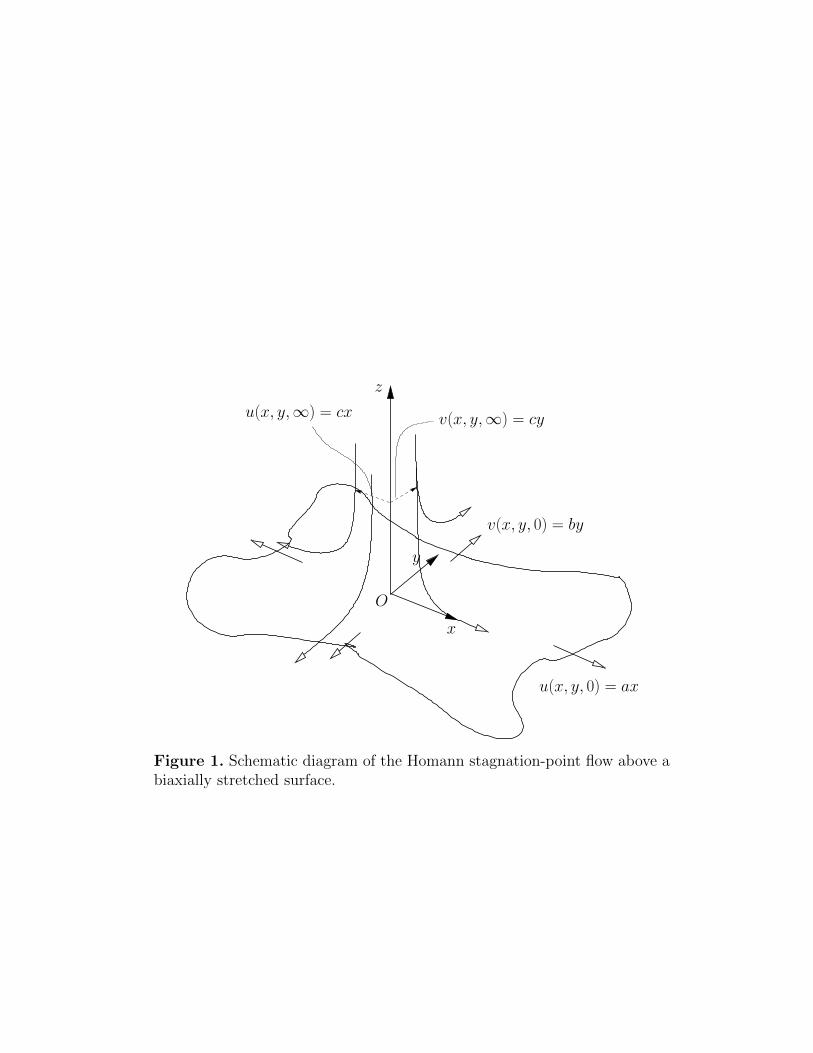
To break the axisymmetry of the Homann stagnation-point flow, we express the variables

in Cartesian coordinates (x,y,z) with corresponding velocities (u,v,w) to attain

u = cx, v = cy, w = −2cz (2.1)

for the flow far from the plate, while the flow on the plate surface is given as

u = ax, v = by, w = 0. (2.2)

A schematic diagram of the flow setup is given in figure 1. Thus the natural choice for

a similarity reduction is

u(x, y, η) = cx f ′(η), v(x, y, η) = cy g′(η), η =

√c

νz (2.3a)

where a prime denotes differentiation with respect to η (Turner and Weidman, 2017).

The continuity equation for an incompressible flow is satisfied by

w(η) = −√cν[f(η) + g(η)]. (2.3b)

Inserting the ansatz (2.3) into the three-dimensional Navier-Stokes equations furnishes

the coupled pair of equations for η ≥ 0 as

f ′′′ + (f + g)f ′′ − f ′2 + 1 = 0, g′′′ + (f + g)g′′ − g′2 + 1 = 0 (2.4a)

to be solved with impermeable stretching wall and far-field conditions

f(0) = 0, f ′(0) = α, f ′(∞) = 1; g(0) = 0, g′(0) = β, g′(∞) = 1 (2.4b)

where α = a/c and β = b/c measure the surface stretching rate in the x- and y-directions

respectively, normalized by the stagnation-point flow strength at infinity.

Integrating the z-component of the Navier-Stokes equation gives an expression for

the pressure field

p(x, y, η) = p0 + ρνc(a+ b)− ρ[c2(x2

2+y2

2

)+ cν

((f + g)2

2+ (f ′ + g′)

)](2.5)

3

in which p0 is the stagnation pressure at x = y = η = 0.

The horizontal shear stresses on the wall are

τx = µ∂u

∂z

∣∣∣∣z=0

= ρν1/2c3/2x f ′′(0) (2.6a)

τy = µ∂v

∂z

∣∣∣∣z=0

= ρν1/2c3/2y g′′(0). (2.6b)

There is an obvious symmetry in the problem obtained by interchanging the x- and

y-axes. This permits interchanging the roles of α and β in numerical computations

presented below.

Furthermore, it is noted that upon setting either α or β equal to zero, one has uni-

lateral stretching beneath axisymmetric Homann stagnation-point flow. This problem,

studied by Turner and Weidman (2017), has a complicated spiral behavior in the shear

stress plane at negative values of the strain rate ratio, where the thickness of the bound-

ary layer increases as one moves along the solution branches into the spiral. Also, when

α = β the surface stretches radially and the flow is everywhere axisymmetric; this is

the problem studied by Weidman and Ma (2016) in which the effect of suction/blowing

through the surface is included. Finally, when α = β = 0 the solution of Homann (1936)

is recovered. Here we present results varying α at fixed values of β 6= 0.

3 Presentation of Results

Equations (2.4a) were integrated numerically in [0, ηmax] using the shooting-splitting

method (Firnett & Troesch, 1974). This method splits the domain [0, ηmax] into N

equally sized sub-domains [ηi, ηi+1] for i = 0, ..., N − 1. In each sub-domain the values

of f = (f, f ′, f ′′, g, g′, g′′) are integrated from ηi to ηi+1 using the 4th order Runge-Kutta

scheme, and the values of f at ηi+1 are updated via Newton iterations using the continuity

of these functions. In the first and final intervals (i = 0 and i = N − 1) the boundary

conditions (2.4b) are applied. This process is repeated until convergence, which for this

work is when ||f (n+1) − f (n)|| < 10−10 where here n denotes the iteration number. The

main benefit of this shooting-splitting procedure over a simple, one-domain shooting

approach is that much larger values of ηmax can be achieved, as the exponential growth

of ‘incorrect’ guesses of f (0) values is restricted to a small domain, making convergence of

the scheme more likely. In the results presented here we use N = 40 and ηmax = 40, and

the value of ηmax was varied to ensure the solutions are independent of the integration

4

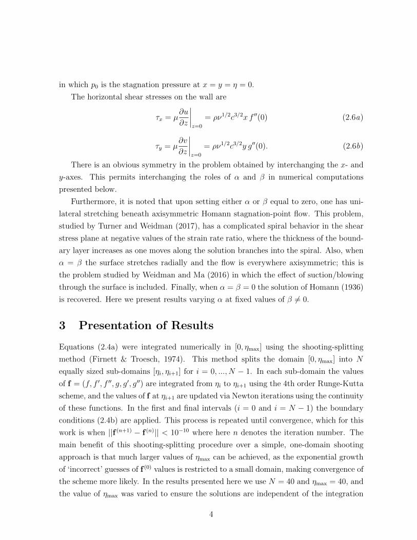
β Branch f ′′(0) g′′(0) β Branch f ′′(0) g′′(0)no. no.

3 1 -3.4937 -4.7940 -0.25 1 -3.0606 1.94423 2 -7.9320 -4.4946 -0.25 2 -.48768 1.75203 3 -3.2666 -8.8871 -0.25 3 -2.8383 -2.17893 4 -7.4809 -4.5978 -0.25 4 -4.7579 1.73612 1 -3.3706 -2.1747 -0.5 1 -3.0218 2.20362 2 -6.9945 -2.0249 -0.5 2 -4.6405 1.97082 3 -3.1483 -6.1546 -0.5 3 -2.7986 -1.99472 4 -6.6621 -2.0967 -0.5 4 -4.5399 1.95971 1 -3.2397 0.0000 -1 1 -2.9401 2.55461 2 -6.0550 0.0000 -1 2 -4.1658 2.23321 3 -3.0204 -3.9392 -1 3 -2.7197 -1.74881 4 -5.8281 -0.0442 -1 4 -4.0982 2.2309

Table 1: Values of f ′′(0) and g′′(0) at α = 2.5 needed to replicate the presented results.

domain size. For an initial guess, we considered the N = 1 interval case and calculated

approximations for f and g at the required η values (η = 1, 2, 3, ... etc), before running

the solver again with N = 40 intervals. Parameter continuation techniques can then be

applied with N = 40 to map out the solution curves of the two key parameters f ′′(0)

and g′′(0), which are found in order to satisfy the far-field conditions f ′(∞) = 1 and

g′(∞) = 1. It is noted at the outset that there are four solution branches for each value

of β, and the values of f ′′(0) and g′′(0) at α = 2.5 required to replicate the results

presented, are given in table 1.

3.1 Case β ≥ 1

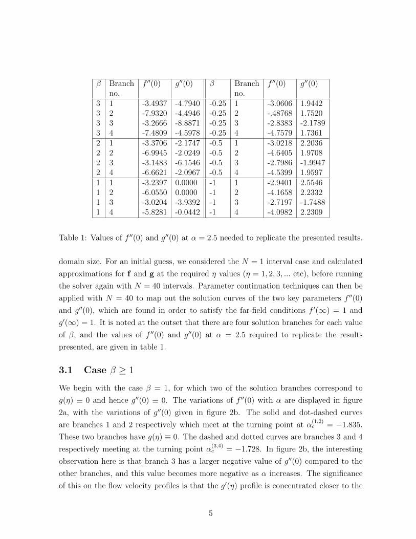
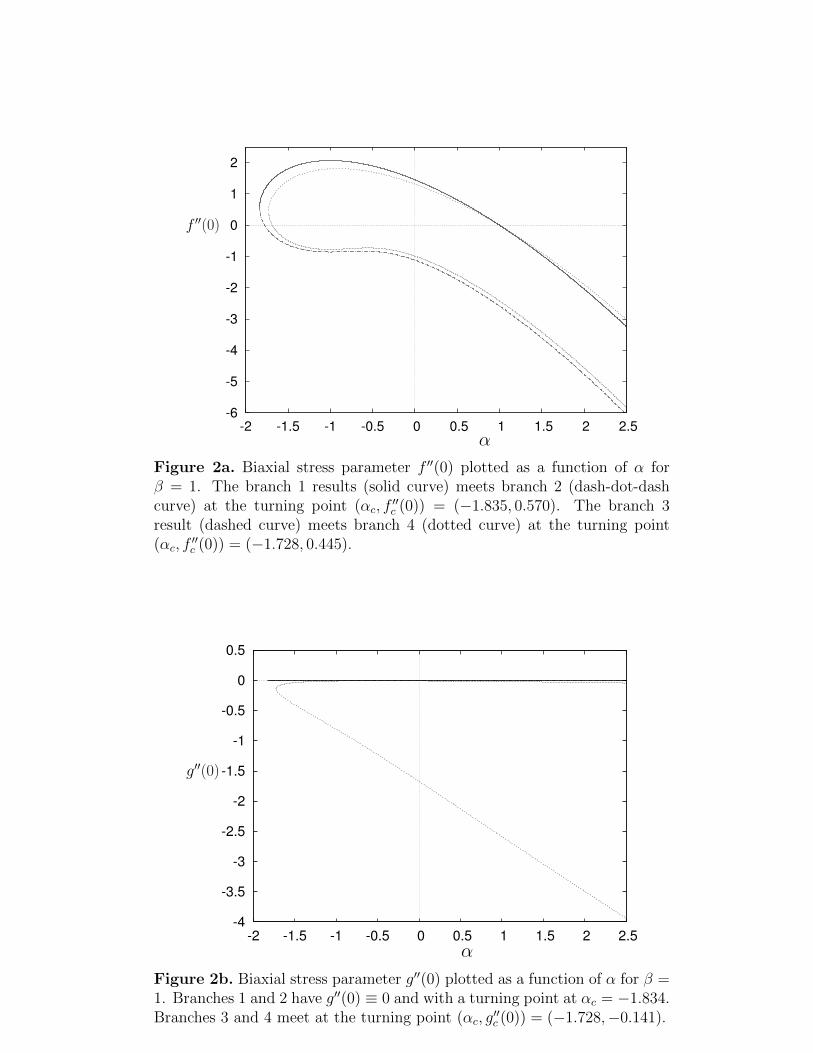
We begin with the case β = 1, for which two of the solution branches correspond to

g(η) ≡ 0 and hence g′′(0) ≡ 0. The variations of f ′′(0) with α are displayed in figure

2a, with the variations of g′′(0) given in figure 2b. The solid and dot-dashed curves

are branches 1 and 2 respectively which meet at the turning point at α(1,2)c = −1.835.

These two branches have g(η) ≡ 0. The dashed and dotted curves are branches 3 and 4

respectively meeting at the turning point α(3,4)c = −1.728. In figure 2b, the interesting

observation here is that branch 3 has a larger negative value of g′′(0) compared to the

other branches, and this value becomes more negative as α increases. The significance

of this on the flow velocity profiles is that the g′(η) profile is concentrated closer to the

5

surface of the plate, this is shown for β = 2 below. Note, throughout the rest of the

presented results we keep with the same plotting convention where branches 1-4 are

represented by solid, dot-dashed, dashed and dotted curves respectively.

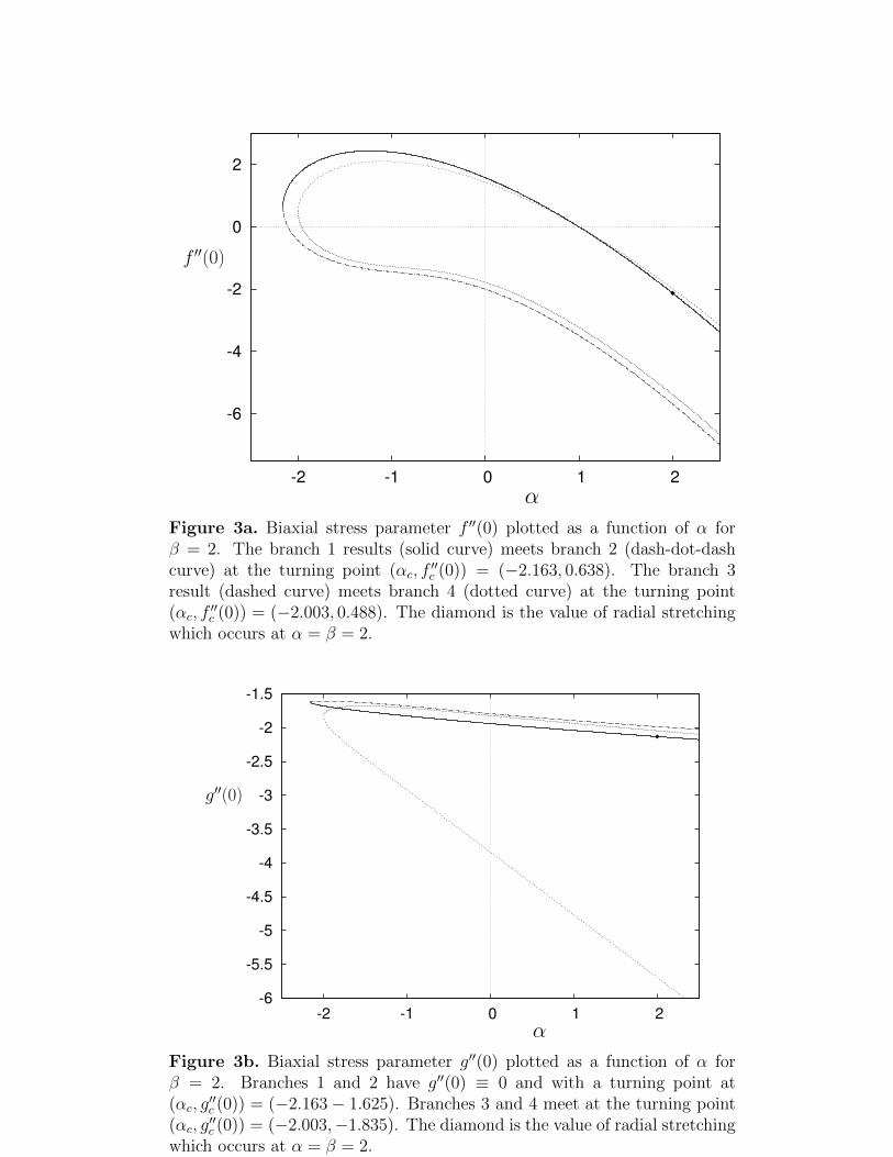
When β = 2, figure 3a shows f ′′(0) plotted as a function of α in which the branch 1

curve the branch 2 meet at the turning point α(1,2)c = −2.163, while the branch 3 curve

meets the branch 4 curve at the turning point α(3,4)c = −2.003. The overall structure of

the results is similar to that in figure 2 for β = 1. Figure 3b shows that this is also the

case for g′′(0) where again the value of |g′′(0)| along branch 3 is larger than on the other

three branches, for which g′′(0) is similar in magnitude. In both figures the diamond is

the value of radial stretching which occurs at α = β = 2.

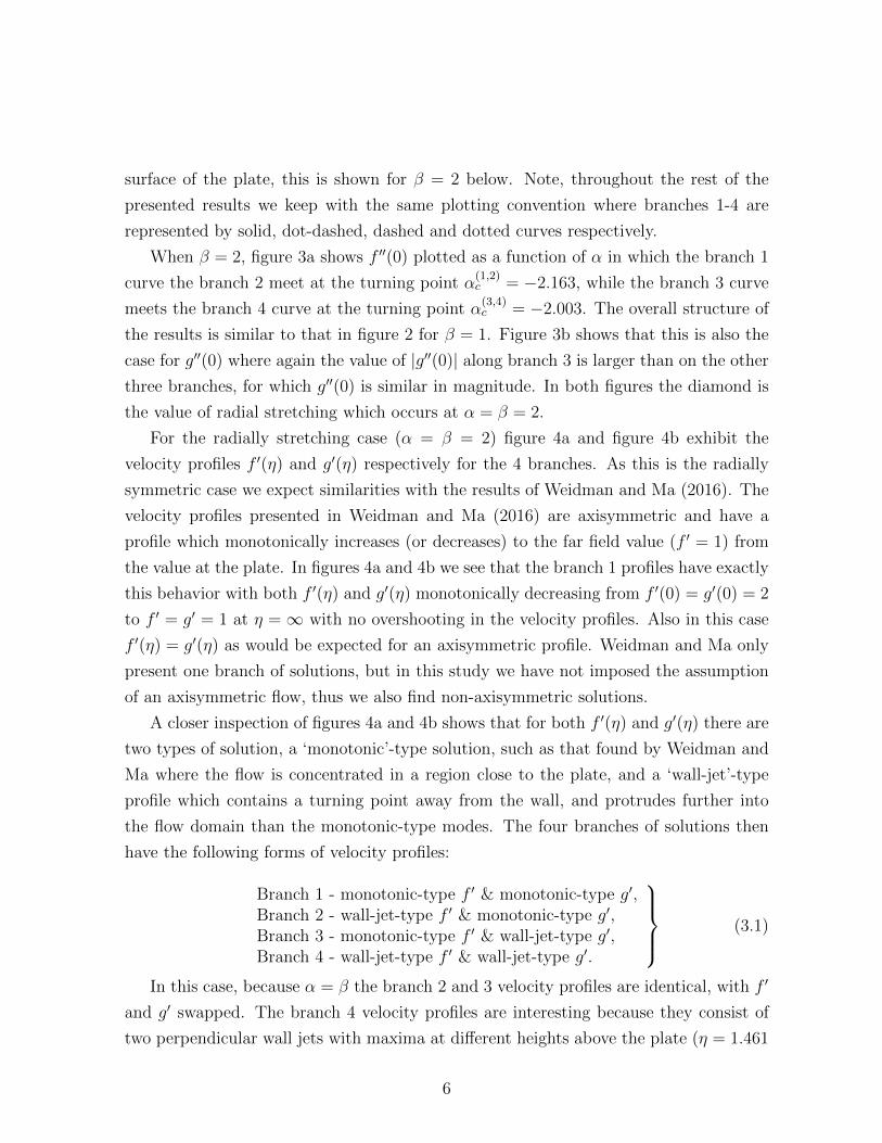
For the radially stretching case (α = β = 2) figure 4a and figure 4b exhibit the

velocity profiles f ′(η) and g′(η) respectively for the 4 branches. As this is the radially

symmetric case we expect similarities with the results of Weidman and Ma (2016). The

velocity profiles presented in Weidman and Ma (2016) are axisymmetric and have a

profile which monotonically increases (or decreases) to the far field value (f ′ = 1) from

the value at the plate. In figures 4a and 4b we see that the branch 1 profiles have exactly

this behavior with both f ′(η) and g′(η) monotonically decreasing from f ′(0) = g′(0) = 2

to f ′ = g′ = 1 at η =∞ with no overshooting in the velocity profiles. Also in this case

f ′(η) = g′(η) as would be expected for an axisymmetric profile. Weidman and Ma only

present one branch of solutions, but in this study we have not imposed the assumption

of an axisymmetric flow, thus we also find non-axisymmetric solutions.

A closer inspection of figures 4a and 4b shows that for both f ′(η) and g′(η) there are

two types of solution, a ‘monotonic’-type solution, such as that found by Weidman and

Ma where the flow is concentrated in a region close to the plate, and a ‘wall-jet’-type

profile which contains a turning point away from the wall, and protrudes further into

the flow domain than the monotonic-type modes. The four branches of solutions then

have the following forms of velocity profiles:

Branch 1 - monotonic-type f ′ & monotonic-type g′,Branch 2 - wall-jet-type f ′ & monotonic-type g′,Branch 3 - monotonic-type f ′ & wall-jet-type g′,Branch 4 - wall-jet-type f ′ & wall-jet-type g′.

(3.1)

In this case, because α = β the branch 2 and 3 velocity profiles are identical, with f ′

and g′ swapped. The branch 4 velocity profiles are interesting because they consist of

two perpendicular wall jets with maxima at different heights above the plate (η = 1.461

6

and η = 5.231).

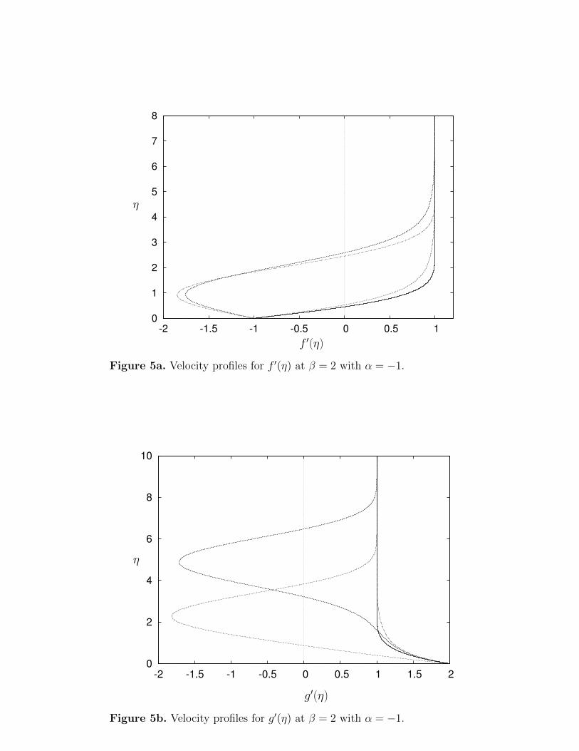
The above structure is valid along the entire branch of solutions, which can be seen

in figures 5a and 5b which show the velocity profiles f ′(η) and g′(η) respectively for

the case β = 2 but with α = −1. Here we observe that as we reduce the value of α

the distance that the solution protrudes away from the plate increases, and it is this

thickening of the flow structure that ultimately leads to there being no solutions for

α < αc.

The final positive β value we consider is β = 3. Figures 6a and 6b show the stress

parameters f ′′(0) and g′′(0) plotted as a function of α. Here the branch 1 and branch

2 solution curves meet at a turning point at α(1,2)c = −2.474, while the branch 3 and

branch 4 curves meet at the turning point α(3,4)c = −2.260. By comparing the cases for

different β values, we see that range of negative values of α (shrinking plates), for which

solutions exist, increases with increasing β.

3.2 Case β < 0

Next, we consider the case β < 0, i.e. the shrinking of the plate in the y-direction.

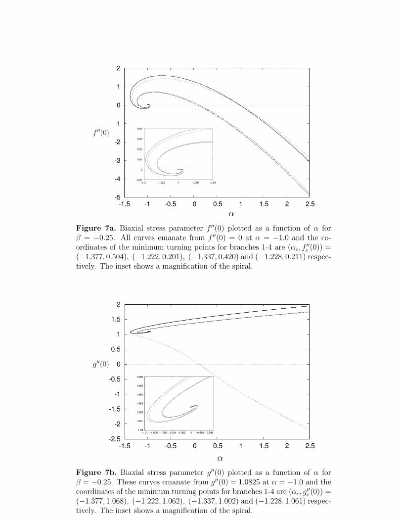
The case β = −0.25 is considered in figures 7a and 7b, which plot f ′′(0) and g′′(0)

respectively as a function of α. For α > 0 the four solution branches for f ′′(0) appear

very similar as for β > 0, however the results for g′′(0) are different. By considering the

results in the previous section we note that for β > 1 all the values of g′′(0) are negative,

and g′′(0) ≡ 0 for branches 1 and 2 when β = 1. As β reduces further, branches 1, 2

and 4 then have g′′(0) > 0 for large positive α, but branch 3 remains with g′′(0) < 0 for

large positive α. In terms of the velocity profiles, this means that g′(η) always has a flow

velocity directed towards the origin which increases in magnitude as the plate surface is

left. This can be seen in figure 8b which plots g′(η) for β = −0.25 and α = 2, with the

corresponding f ′(η) plots given in figure 8a. As for β = 2, the profiles are again either

of monotonic-type or wall-jet-type and the branch solutions again satisfy (3.1).

For α < 0 in figures 7a and 7b the solution curves no longer meet at a turning

point, and instead each solution curve spirals in to a point in the (α, f ′′(0), g′′(0)) pa-

rameter space, as was observed in Turner and Weidman (2017) for the case β = 0.

The minimum turning point values denoting the boundary of possible solutions for each

branch are α(1)c = −1.377 for branch 1, α

(2)c = −1.222 for branch 2, α

(3)c = −1.337 for

branch 3 and α(4)c = −1.228 for branch 4. The center of the spiral for β = −0.25 is at

(α, f ′′(0), g′′(0)) = (−1, 0, 1.086).

7

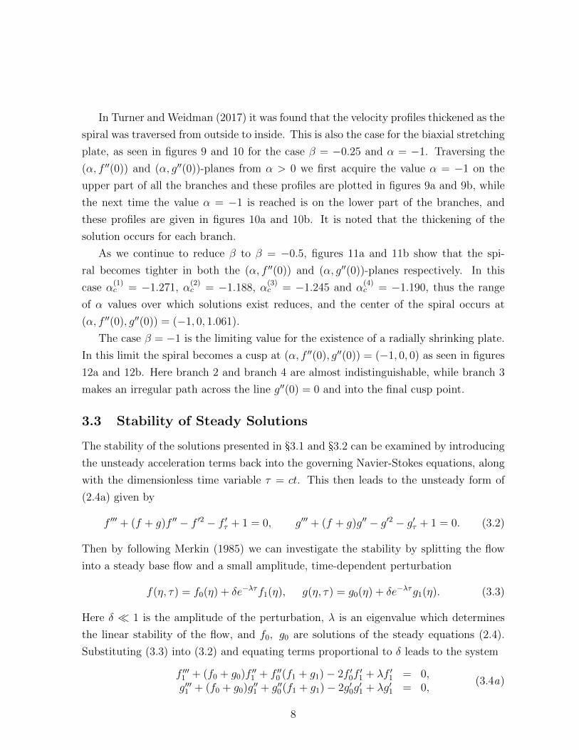
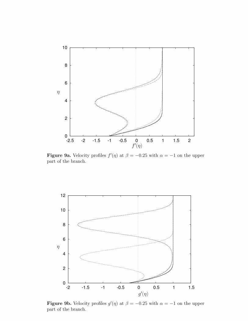
In Turner and Weidman (2017) it was found that the velocity profiles thickened as the

spiral was traversed from outside to inside. This is also the case for the biaxial stretching

plate, as seen in figures 9 and 10 for the case β = −0.25 and α = −1. Traversing the

(α, f ′′(0)) and (α, g′′(0))-planes from α > 0 we first acquire the value α = −1 on the

upper part of all the branches and these profiles are plotted in figures 9a and 9b, while

the next time the value α = −1 is reached is on the lower part of the branches, and

these profiles are given in figures 10a and 10b. It is noted that the thickening of the

solution occurs for each branch.

As we continue to reduce β to β = −0.5, figures 11a and 11b show that the spi-

ral becomes tighter in both the (α, f ′′(0)) and (α, g′′(0))-planes respectively. In this

case α(1)c = −1.271, α

(2)c = −1.188, α

(3)c = −1.245 and α

(4)c = −1.190, thus the range

of α values over which solutions exist reduces, and the center of the spiral occurs at

(α, f ′′(0), g′′(0)) = (−1, 0, 1.061).

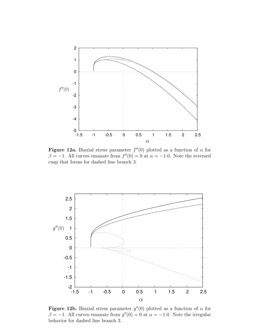
The case β = −1 is the limiting value for the existence of a radially shrinking plate.

In this limit the spiral becomes a cusp at (α, f ′′(0), g′′(0)) = (−1, 0, 0) as seen in figures

12a and 12b. Here branch 2 and branch 4 are almost indistinguishable, while branch 3

makes an irregular path across the line g′′(0) = 0 and into the final cusp point.

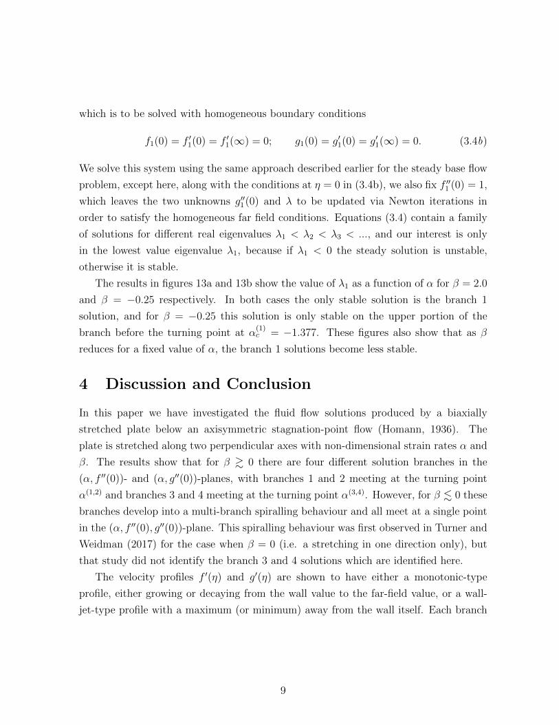
3.3 Stability of Steady Solutions

The stability of the solutions presented in §3.1 and §3.2 can be examined by introducing

the unsteady acceleration terms back into the governing Navier-Stokes equations, along

with the dimensionless time variable τ = ct. This then leads to the unsteady form of

(2.4a) given by

f ′′′ + (f + g)f ′′ − f ′2 − f ′τ + 1 = 0, g′′′ + (f + g)g′′ − g′2 − g′τ + 1 = 0. (3.2)

Then by following Merkin (1985) we can investigate the stability by splitting the flow

into a steady base flow and a small amplitude, time-dependent perturbation

f(η, τ) = f0(η) + δe−λτf1(η), g(η, τ) = g0(η) + δe−λτg1(η). (3.3)

Here δ � 1 is the amplitude of the perturbation, λ is an eigenvalue which determines

the linear stability of the flow, and f0, g0 are solutions of the steady equations (2.4).

Substituting (3.3) into (3.2) and equating terms proportional to δ leads to the system

f ′′′1 + (f0 + g0)f′′1 + f ′′0 (f1 + g1)− 2f ′0f

′1 + λf ′1 = 0,

g′′′1 + (f0 + g0)g′′1 + g′′0(f1 + g1)− 2g′0g

′1 + λg′1 = 0,

(3.4a)

8

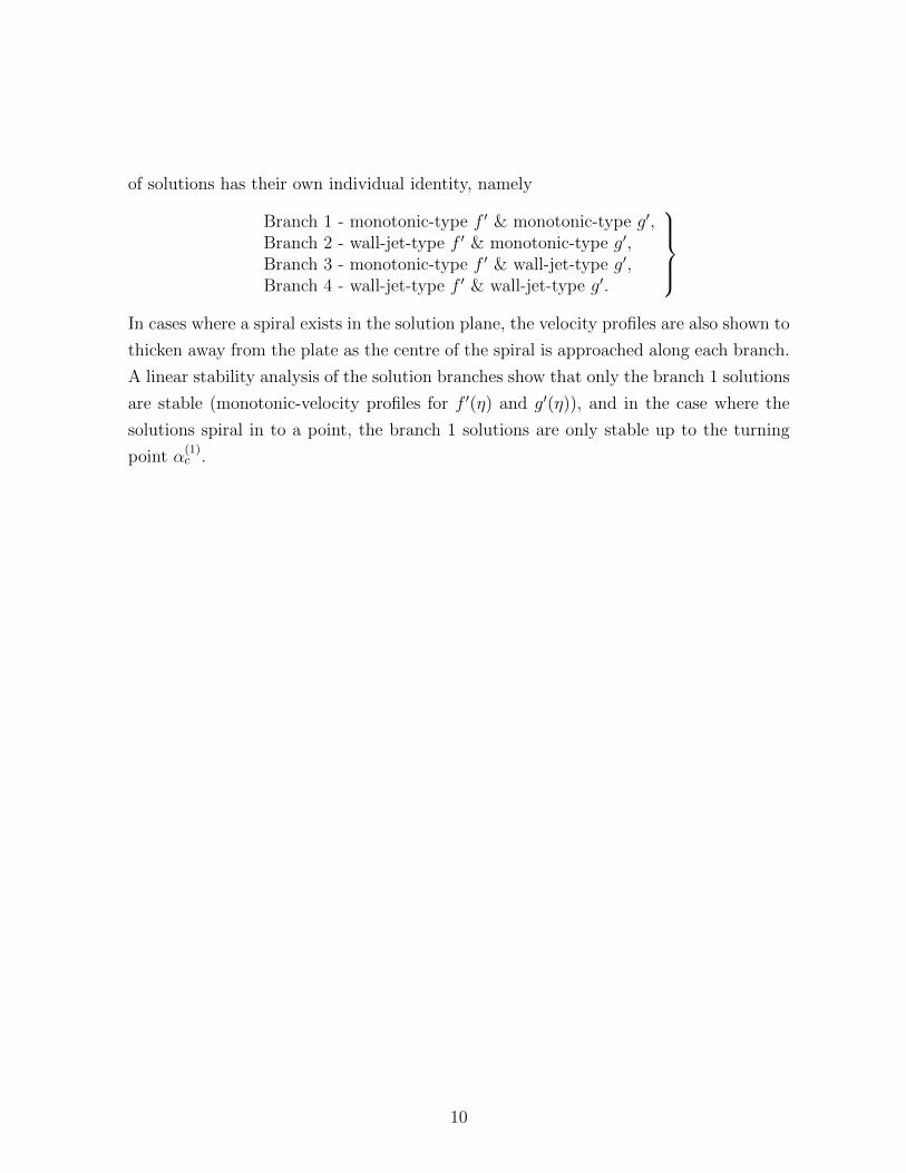
which is to be solved with homogeneous boundary conditions

f1(0) = f ′1(0) = f ′1(∞) = 0; g1(0) = g′1(0) = g′1(∞) = 0. (3.4b)

We solve this system using the same approach described earlier for the steady base flow

problem, except here, along with the conditions at η = 0 in (3.4b), we also fix f ′′1 (0) = 1,

which leaves the two unknowns g′′1(0) and λ to be updated via Newton iterations in

order to satisfy the homogeneous far field conditions. Equations (3.4) contain a family

of solutions for different real eigenvalues λ1 < λ2 < λ3 < ..., and our interest is only

in the lowest value eigenvalue λ1, because if λ1 < 0 the steady solution is unstable,

otherwise it is stable.

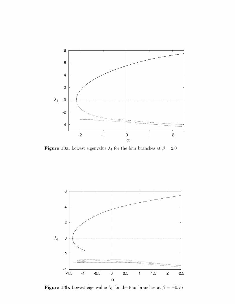
The results in figures 13a and 13b show the value of λ1 as a function of α for β = 2.0

and β = −0.25 respectively. In both cases the only stable solution is the branch 1

solution, and for β = −0.25 this solution is only stable on the upper portion of the

branch before the turning point at α(1)c = −1.377. These figures also show that as β

reduces for a fixed value of α, the branch 1 solutions become less stable.

4 Discussion and Conclusion

In this paper we have investigated the fluid flow solutions produced by a biaxially

stretched plate below an axisymmetric stagnation-point flow (Homann, 1936). The

plate is stretched along two perpendicular axes with non-dimensional strain rates α and

β. The results show that for β & 0 there are four different solution branches in the

(α, f ′′(0))- and (α, g′′(0))-planes, with branches 1 and 2 meeting at the turning point

α(1,2) and branches 3 and 4 meeting at the turning point α(3,4). However, for β . 0 these

branches develop into a multi-branch spiralling behaviour and all meet at a single point

in the (α, f ′′(0), g′′(0))-plane. This spiralling behaviour was first observed in Turner and

Weidman (2017) for the case when β = 0 (i.e. a stretching in one direction only), but

that study did not identify the branch 3 and 4 solutions which are identified here.

The velocity profiles f ′(η) and g′(η) are shown to have either a monotonic-type

profile, either growing or decaying from the wall value to the far-field value, or a wall-

jet-type profile with a maximum (or minimum) away from the wall itself. Each branch

9

of solutions has their own individual identity, namely

Branch 1 - monotonic-type f ′ & monotonic-type g′,Branch 2 - wall-jet-type f ′ & monotonic-type g′,Branch 3 - monotonic-type f ′ & wall-jet-type g′,Branch 4 - wall-jet-type f ′ & wall-jet-type g′.

In cases where a spiral exists in the solution plane, the velocity profiles are also shown to

thicken away from the plate as the centre of the spiral is approached along each branch.

A linear stability analysis of the solution branches show that only the branch 1 solutions

are stable (monotonic-velocity profiles for f ′(η) and g′(η)), and in the case where the

solutions spiral in to a point, the branch 1 solutions are only stable up to the turning

point α(1)c .

10

References

Attia, H. A., Homann magnetic flow and heat transfer with uniform suction or injection,

Can. J. Phys., 81, 1223–1230 (2003).

Drazin, P. and Riley, N., The Navier-Stokes Equations: A Classification of Flows and

Exact Solutions, London Mathematical Society Lecture Note Series 334 (Cambridge

University Press, 2006).

Firnett, P. J. and Troesch, B. A., Shooting-splitting method for sensitive two-point

boundary value problems, In: Bettis D.G. (eds) Proceedings of the Conference on the

Numerical Solution of Ordinary Differential Equations, 362, 408-433 (Springer-Verlag,

Berlin, 1974).

Homann, F. Der Einfluss grosser Zahigkeit bei der Stromung um den Zylinder und um

die Kugel, Z. angew. Math. Mech. (ZAMM), 16, 153-164 (1936).

Mahapatra, T. R. and Gupta, A. S., Stagnation-point flow towards a stretching sheet,

Can. J. Chem. Eng., 81, 258–263 (2003).

Merkin, J. H., On dual solutions occurring in mixed convection in a porous medium. J.

Engng. Math., 20, 171-179 (1985).

Turner, M. R. and Weidman, P. D., Stagnation-point flow with stretching surfaces: A

unified formulation and new results Euro. J. Mech. B/Fluids, 61, 144-153 (2017).

Wang, C. Y. Similarity stagnation point solutions of the Navier-Stokes equations —

review and extension, Eur. J. Mech. B/Fluids, 27, 678-683 (2008).

Weidman, P. D., Hiemenz stagnation-point flow impinging on a biaxially stretching

surface, Meccanica, 53, 833–840 (2018)

Weidman, P. D. and Ma, Y., The competing effects of wall transpiration and stretching

on Homann stagnation-point flow, Eur. J. Mech. B/Fluids, 60, 237–241 (2016)

Weidman, P. D. and Mahalingam, S., Axisymmetric stagnation-point flow impinging in

a transversely oscillating plate with suction, J. Engrg. Math., 31, 305-318 (1997).

11

u(x, y, 0) = ax

v(x, y, 0) = by

u(x, y,∞) = cx v(x, y,∞) = cy

x

y

z

O

Figure 1. Schematic diagram of the Homann stagnation-point flow above abiaxially stretched surface.

12

-6

-5

-4

-3

-2

-1

0

1

2

-2 -1.5 -1 -0.5 0 0.5 1 1.5 2 2.5

α

f ′′(0)

Figure 2a. Biaxial stress parameter f ′′(0) plotted as a function of α forβ = 1. The branch 1 results (solid curve) meets branch 2 (dash-dot-dashcurve) at the turning point (αc, f

′′c (0)) = (−1.835, 0.570). The branch 3

result (dashed curve) meets branch 4 (dotted curve) at the turning point(αc, f

′′c (0)) = (−1.728, 0.445).

-4

-3.5

-3

-2.5

-2

-1.5

-1

-0.5

0

0.5

-2 -1.5 -1 -0.5 0 0.5 1 1.5 2 2.5

α

g′′(0)

Figure 2b. Biaxial stress parameter g′′(0) plotted as a function of α for β =1. Branches 1 and 2 have g′′(0) ≡ 0 and with a turning point at αc = −1.834.Branches 3 and 4 meet at the turning point (αc, g

′′c (0)) = (−1.728,−0.141).

13

-6

-4

-2

0

2

-2 -1 0 1 2

α

f ′′(0)

Figure 3a. Biaxial stress parameter f ′′(0) plotted as a function of α forβ = 2. The branch 1 results (solid curve) meets branch 2 (dash-dot-dashcurve) at the turning point (αc, f

′′c (0)) = (−2.163, 0.638). The branch 3

result (dashed curve) meets branch 4 (dotted curve) at the turning point(αc, f

′′c (0)) = (−2.003, 0.488). The diamond is the value of radial stretching

which occurs at α = β = 2.

-6

-5.5

-5

-4.5

-4

-3.5

-3

-2.5

-2

-1.5

-2 -1 0 1 2

α

g′′(0)

Figure 3b. Biaxial stress parameter g′′(0) plotted as a function of α forβ = 2. Branches 1 and 2 have g′′(0) ≡ 0 and with a turning point at(αc, g

′′c (0)) = (−2.163− 1.625). Branches 3 and 4 meet at the turning point

(αc, g′′c (0)) = (−2.003,−1.835). The diamond is the value of radial stretching

which occurs at α = β = 2.

14

0

1

2

3

4

5

6

7

8

-2.5 -2 -1.5 -1 -0.5 0 0.5 1 1.5 2

η

f ′(η)

Figure 4a. Velocity profiles for f ′(η) at β = 2 with α = 2.

0

2

4

6

8

10

-2.5 -2 -1.5 -1 -0.5 0 0.5 1 1.5 2

η

g′(η)

Figure 4b. Velocity profiles g′(η) at β = 2 with α = 2.

15

0

1

2

3

4

5

6

7

8

-2 -1.5 -1 -0.5 0 0.5 1

η

f ′(η)

Figure 5a. Velocity profiles for f ′(η) at β = 2 with α = −1.

0

2

4

6

8

10

-2 -1.5 -1 -0.5 0 0.5 1 1.5 2

η

g′(η)

Figure 5b. Velocity profiles for g′(η) at β = 2 with α = −1.

16

-6

-4

-2

0

2

-2 -1 0 1 2

α

f ′′(0)

Figure 6a. Biaxial stress parameter f ′′(0) plotted as a function of α forβ = 3. The branch 1 results (solid curve) meets branch 2 (dash-dot-dashcurve) at the turning point (αc, f

′′c (0)) = (−2.474, 0.715). The branch 3

result (dashed curve) meets branch 4 (dotted curve) at the turning point(αc, f

′′c (0)) = (−2.260, 0.538).

-9

-8

-7

-6

-5

-4

-2 -1 0 1 2

α

g′′(0)

Figure 6b. Biaxial stress parameter g′′(0) plotted as a function of α forβ = 3. Branches 1 and 2 have g′′(0) ≡ 0 and with a turning point at(αc, g

′′c (0)) = (−2.474,−3.737). Branches 3 and 4 meet at the turning point

(αc, g′′c (0)) = (−2.260,−4.021).

17

-5

-4

-3

-2

-1

0

1

2

-1.5 -1 -0.5 0 0.5 1 1.5 2 2.5

α

f ′′(0)

-0.01

0

0.01

0.02

0.03

0.04

-1.01 -1.005 -1 -0.995 -0.99

Figure 7a. Biaxial stress parameter f ′′(0) plotted as a function of α forβ = −0.25. All curves emanate from f ′′(0) = 0 at α = −1.0 and the co-ordinates of the minimum turning points for branches 1-4 are (αc, f

′′c (0)) =

(−1.377, 0.504), (−1.222, 0.201), (−1.337, 0.420) and (−1.228, 0.211) respec-tively. The inset shows a magnification of the spiral.

-2.5

-2

-1.5

-1

-0.5

0

0.5

1

1.5

2

-1.5 -1 -0.5 0 0.5 1 1.5 2 2.5

α

g′′(0)

1.08

1.081

1.082

1.083

1.084

1.085

1.086

-1.01 -1.008 -1.006 -1.004 -1.002 -1 -0.998 -0.996

Figure 7b. Biaxial stress parameter g′′(0) plotted as a function of α forβ = −0.25. These curves emanate from g′′(0) = 1.0825 at α = −1.0 and thecoordinates of the minimum turning points for branches 1-4 are (αc, g

′′c (0)) =

(−1.377, 1.068), (−1.222, 1.062), (−1.337, 1.002) and (−1.228, 1.061) respec-tively. The inset shows a magnification of the spiral.

18

0

1

2

3

4

5

6

7

8

-2 -1.5 -1 -0.5 0 0.5 1 1.5 2

η

f ′(η)

Figure 8a. Velocity profiles f ′(η) at β = −0.25 with α = 2.

0

2

4

6

8

10

-2 -1.5 -1 -0.5 0 0.5 1

η

g′(η)

Figure 8b. Velocity profiles g′(η) at β = −0.25 with α = 2.

19

0

2

4

6

8

10

-2.5 -2 -1.5 -1 -0.5 0 0.5 1 1.5 2

η

f ′(η)

Figure 9a. Velocity profiles f ′(η) at β = −0.25 with α = −1 on the upperpart of the branch.

0

2

4

6

8

10

12

-2 -1.5 -1 -0.5 0 0.5 1 1.5

η

g′(η)

Figure 9b. Velocity profiles g′(η) at β = −0.25 with α = −1 on the upperpart of the branch.

20

0

2

4

6

8

10

12

-2 -1.5 -1 -0.5 0 0.5 1

η

f ′(η)

Figure 10a. Velocity profiles f ′(η) at β = −0.25 with α = −1 on the lowerpart of the branch.

0

2

4

6

8

10

12

14

-2 -1.5 -1 -0.5 0 0.5 1

η

g′(η)

Figure 10b. Velocity profiles g′(η) at β = −0.25 with α = −1 on the lowerpart of the branch.

21

-5

-4

-3

-2

-1

0

1

2

-1.5 -1 -0.5 0 0.5 1 1.5 2 2.5

α

f ′′(0)

Figure 11a. Biaxial stress parameter f ′′(0) plotted as a function of α forβ = −0.5. All curves emanate from f ′′(0) = 0 at α = −1.0 and the co-ordinates of the minimum turning points for branches 1-4 are (αc, f

′′c (0)) =

(−1.271, 0.478), (−1.188, 0.266), (−1.245, 0.447) and (−1.190, 0.283) respec-tively.

-2

-1.5

-1

-0.5

0

0.5

1

1.5

2

2.5

-1.5 -1 -0.5 0 0.5 1 1.5 2 2.5

α

g′′(0)

Figure 11b. Biaxial stress parameter g′′(0) plotted as a function of α forβ = −0.5. These curves emanate from g′′(0) = 1.0606 at α = −1 and thecoordinates of the minimum turning points for branches 1-4 are (αc, g

′′c (0)) =

(−1.271, 1.075), (−1.188, 1.058), (−1.245, 1.026) and (−1.190, 1.060) respec-tively.

22

-5

-4

-3

-2

-1

0

1

2

-1.5 -1 -0.5 0 0.5 1 1.5 2 2.5

α

f ′′(0)

Figure 12a. Biaxial stress parameter f ′′(0) plotted as a function of α forβ = −1. All curves emanate from f ′′(0) = 0 at α = −1.0. Note the reversedcusp that forms for dashed line branch 3.

-2

-1.5

-1

-0.5

0

0.5

1

1.5

2

2.5

-1.5 -1 -0.5 0 0.5 1 1.5 2 2.5

α

g′′(0)

Figure 12b. Biaxial stress parameter g′′(0) plotted as a function of α forβ = −1. All curves emanate from g′′(0) = 0 at α = −1.0. Note the irregularbehavior for dashed line branch 3.

23

-4

-2

0

2

4

6

8

-2 -1 0 1 2

α

λ1

Figure 13a. Lowest eigenvalue λ1 for the four branches at β = 2.0

-4

-2

0

2

4

6

-1.5 -1 -0.5 0 0.5 1 1.5 2 2.5

α

λ1

Figure 13b. Lowest eigenvalue λ1 for the four branches at β = −0.25

24