Embed Size (px)
Citation preview

UT-Komaba/18-6
Prepared for submission to JHEP arXiv:1901.nnnnn [hep-th]
Holographic Complexity Equals Which Action?
Kanato Goto,a Hugo Marrochio,b,c Robert C Myers,b Leonel Queimadab,c and
Beni Yoshidab
aThe University of Tokyo, Komaba, Meguro-ku, Tokyo 153-8902 JapanbPerimeter Institute for Theoretical Physics, Waterloo, ON N2L 2Y5, CanadacDepartment of Physics & Astronomy, University of Waterloo,
Waterloo, ON N2L 3G1, Canada
E-mail: [email protected],
[email protected], [email protected],
Abstract: We revisit the complexity=action proposal for charged black holes. We in-
vestigate the complexity for a dyonic black hole, and we find the surprising feature that
the late-time growth is sensitive to the ratio between electric and magnetic charges.
In particular, the late-time growth rate vanishes when the black hole carries only a
magnetic charge. If the dyonic black hole is perturbed by a light shock wave, a similar
feature appears for the switchback effect, e.g., it is absent for purely magnetic black
holes. We then show how the inclusion of a surface term to the action can put the elec-
tric and magnetic charges on an equal footing, or more generally change the value of
the late-time growth rate. Next, we investigate how the causal structure influences the
late-time growth with and without the surface term for charged black holes in a fam-
ily of Einstein-Maxwell-Dilaton theories. Finally, we connect the previous discussion
to the complexity=action proposal for the two-dimensional Jackiw-Teitelboim theory.
Since the two-dimensional theory is obtained by a dimensional reduction from Einstein-
Maxwell theory in higher dimensions in a near-extremal and near-horizon limit, the
choices of parent action and parent background solution determine the behaviour of
holographic complexity in two dimensions.
arX
iv:1
901.
0001
4v1
[he
p-th
] 3
1 D
ec 2
018

Contents
1 Introduction 1
2 Reissner-Nordstrom Black Hole 5
2.1 Complexity Growth 7
2.2 Maxwell Boundary Term 11
2.3 Shock Wave Geometries 14
3 Charged Dilatonic Black Hole 20
3.1 Complexity Growth 23
3.2 Boundary Terms 27
4 Black Holes in Two Dimensions 30
4.1 Jackiw-Teitelboim Model 31
4.2 JT-like Model 37
4.3 Boundary Terms? 41
5 Discussion 44
A More on Shock Waves 51
B Bulk Contribution from Maxwell Boundary Term 55
1 Introduction
Recent years have witnessed that quantum information theoretic notions shed new
light on deep conceptual puzzles in the AdS/CFT correspondence, and also provide
useful tools to study the dynamics of strongly-coupled quantum field theories, e.g.,
[1–12]. One striking, yet mysterious, entry to the gravity/information dictionary is the
concept of quantum circuit complexity: the size of the optimal circuit which prepares
a target state from a given reference state with a set of “simple” gates [13–16]. The
concept of holographic complexity naturally emerges from considerations on the bulk
causality in the AdS/CFT correspondence [17]. For instance, holographic complexity
is expected to be a useful diagnostic for late-time dynamics and in particular, the
interior of a black hole since it continues to increase even after the boundary theory
– 1 –

has reached thermal equilibrium. In addition, complexity is sensitive to perturbations
of the system, namely the physics of scrambling, i.e., even tiny perturbations to the
system have a measurable effect on the complexity [17].
The original proposal for holographic complexity, known as the complexity=volume
(CV) conjecture, asserts that [17, 18]
CV(Σ) = maxΣ=∂B
[V(B)
GN L
], (1.1)
where the boundary state lives on the time slice Σ and then V(B) is the volume of
codimension-one bulk surfaces B anchored to this boundary time slice. To produce
a dimensionless quantity, the volume is divided by Newton’s constant GN and the
AdS length L.1 A second proposal, known as the complexity=action (CA) conjecture,
relates the complexity of the boundary state to the gravitational action evaluated for
a particular region of the bulk spacetime [20, 21]
CA(Σ) =IWDW
π ~. (1.2)
Here, the subscript WDW indicates that the action is calculated on the so-called
Wheeler-DeWitt patch, which corresponds to the causal development of any of the
above bulk surfaces B anchored on Σ.
The study of holographic complexity is actively developing in two related directions.
The first is to explore the properties of the new gravitational observables which play a
role in the CV and CA conjectures and the implications of these conjectures for com-
plexity in the boundary theory, e.g., see [17–55]. In particular, we note that a number of
new proposals have been made for the holographic dual of complexity in the boundary
theory. For example, one new proposal is known as the complexity=(spacetime volume)
(or CV2.0) conjecture, which suggests that the bulk dual of complexity is the spacetime
volume of the WDW patch [53]. Further, more recently, a relation was conjectured be-
tween momentum of an infalling object in the bulk radial direction and complexity of
the corresponding time-evolved operator on the boundary [54, 55]. A second direction
of investigation has been to understand the concept of circuit complexity for quantum
field theory states, in particular for states in a strongly coupled CFT, e.g., see [56–73]
Developing a proper understanding of complexity in the boundary theory is essential to
properly test the various holographic proposals and ultimately, to produce a derivation
of one (or more) of these conjectures.
Our motivation for the present paper was to understand holographic complexity
(and in particular, the CA proposal) in the two-dimensional Jackiw-Teitelboim (JT)
1A more sophisticated approach to choosing the latter scale was described in [19].
– 2 –

model of dilaton-gravity [74, 75]. Recently, there has been a great deal of interest in
the JT model, as it emerges in the holographic description of the Sachdev-Ye-Kitaev
(SYK) model in a particular low energy limit, where the system acquires an emergent
reparametrization invariance [76–87]. Furthermore, the JT gravity exhibits the late-
time behavior of the spectral form factor which are natural from the perspective of
random matrix theory, e.g., [88, 89]. As such, the JT model should be an ideal plat-
form to study the complexity in various dynamical settings and investigate further the
implications of holographic complexity. However, our initial calculation of holographic
complexity in the JT model using the CA proposal (1.2) produced the surprising result
that the growth rate vanishes at late times — see section 4. This result, of course, in
tension with our common expectations for complexity. It can be argued quite generally
that at late times, the complexity should continue to grow with a rate given by [17, 22]
dCdt∼ S T , (1.3)
where the entropy S gives an account of the number of degrees of freedom while the
temperature T sets the scale for the rate at which new gates are introduced. Further
since the JT model is supposed to capture the physics of the SYK model, which exhibits
maximal chaos, we would certainly expect the complexity should increase as fast as it
possibly can. Rather than considering the CA prescription of holographic complexity,
one can also examine the CV proposal (1.1) in this setting and in this case, we found
the extremal volume (i.e., the length of the geodesic connecting the boundary points
defining Σ) continues to grow at a constant rate for arbitrarily late times.
This apparent failure of the CA proposal motivated us to re-examine holographic
complexity for charged black holes in higher dimensions since the JT model can be de-
rived from an appropriate dimensional reduction, e.g., [85–87, 90–93]. In particular, JT
dilaton-gravity describes the near-horizon physics of certain near-extremal black holes
in higher dimensions. Previous studies of holographic complexity of charged black holes,
e.g., [20, 21, 30, 34], had not shown any odd behaviour for the CA proposal. However,
with hindsight, we note that all of these investigations involved electrically charged
black holes, whereas the usual dimensional reduction made to derive the JT model
involves black holes carrying a magnetic charge, e.g., [87, 90]. Our first calculation
in the following is to examine holographic complexity for a dyonic black hole (in four
dimensions) with both electric and magnetic charges. In this case, even if the geometry
is held fixed, we find that the complexity growth rate is very sensitive to the ratio
between the two types of charge. In particular, if the black hole is purely magnetic, we
find that CA proposal yields a vanishing growth rate at late times, and further, that
the switchback effect is absent. Of course, this vanishing matches our result for the JT
– 3 –

model, which would arise in the dimensional reduction of these magnetic black holes.
However, there is a boundary term involving the Maxwell field, which one might
add to the gravitational action. This term arises naturally in the context of black
hole thermodynamics [94] (see also [95, 96]) when defining different thermodynamics
ensemble, i.e., a canonical ensemble with fixed charge, as opposed to a grand canonical
ensemble with fixed chemical potential. We find that with the CA proposal, the holo-
graphic complexity is also sensitive to the introduction of this Maxwell surface term.
In particular, the late-time growth rate is nonvanishing for magnetic black holes with
this surface term, while tuning the coefficient of the surface term can yield a vanishing
growth rate in the electrically charged case. Given these results, we are then lead to
re-examine the dimensional reduction in the presence of the Maxwell surface term and
the behaviour of the corresponding holographic complexity for the JT model and for a
related “JT-like” model, derived from the reduction of electrically charged black holes.
To better understand the vanishing of the complexity growth for the magnetic
black holes, we might also ask whether this result is special to the Einstein-Maxwell
theory. Alternatively, the question can be phrased as which features of the correspond-
ing Reissner-Nordstrom-AdS black holes are important in controlling the behaviour
of the holographic complexity for the CA proposal. As a step in this direction, we
also investigate holographic complexity for charged black holes in a family of four-
dimensional Einstein-Maxwell-Dilaton theories. Holographic complexity of Einstein-
Maxwell-Dilaton theories has been previously studied for several models [30, 36–39].
In these theories, the Maxwell field is coupled to a scalar field (the dilaton) and as a
result, the charged black holes also carry “scalar hair.” With the dilaton excited in
these solutions, the nature of the spacetime singularities and the casual structure of
the corresponding black holes can be modified. Hence we can investigate to what ex-
tent these changes to the spacetime geometry modify the behaviour of the holographic
complexity. Our conclusion will be that the causal structure of the spacetime geometry
is the essential feature leading to the unusual (i.e., vanishing) late-time growth rate
with the CA proposal.
The remainder of our paper is organized as follows: In section 2, we study the CA
proposal for dyonic black holes carrying both electric and magnetic charges in four bulk
dimensions. We first show how for a fixed geometry, the complexity rate of change is
sensitive to the ratio between electric and magnetic charges. We also show how the
inclusion of the Maxwell surface term to the action can also have a dramatic effect on
the late-time growth rate for the CA proposal. In addition, we also briefly investigate
the switchback effect by injecting small shockwaves into the dyonic black hole. In
section 3, we investigate holographic complexity for charged black holes in a family of
Einstein-Maxwell-Dilaton theories. In section 4, we return to holographic complexity
– 4 –

for two-dimensional black holes. In particular, we show that the late-time growth rate
vanishes for the JT model, but that this situation can be ameliorated if the Maxwell
surface term is included in reduction from four to two dimensions. We summarize our
findings and consider their implications in section 5, as well as discussing some possible
future directions. We leave certain technical details to the appendices. In appendix
A, we describe in more detail the calculations of the holographic complexity in the
dyonic shock wave geometries. In appendix B, we comment on subtleties concerning
the evaluation of the Maxwell surface term when magnetic charges are present.
As this project was nearing its completion, we became aware of [97], which has
significant overlap with the present paper. We also add that an independent approach
to understanding holographic complexity for the JT model recently appeared in [98, 99].
2 Reissner-Nordstrom Black Hole
In this section, we investigate applying the complexity=action (CA) conjecture [20, 21]
to evaluate the holographic complexity of the dyonic Reissner-Nordstrom black hole,
while focusing on the Einstein-Maxwell theory in four bulk dimensions, i.e., d = 3 for
the boundary theory. These results are easily extended to general dimensions, if one
also couples the gravity theory to a (d–2)-form potential field (i.e., the Hodge dual of the
one-form Maxwell potential). Our main objective is to understand the effect of a new
boundary term associated with the Maxwell field. As mentioned in the introduction,
we will find that although this boundary term does not modify the field equations, it
has a strong influence on the action of the Wheeler-DeWitt (WDW) patch. Hence we
must ask which choices (for the coefficient of this term) yield a WDW action which
produces the behaviours expected of holographic complexity.
We divide the action for four-dimensional Einstein-Maxwell theory in terms of the
usual Einstein-Hilbert and Maxwell actions, as well as various possible surface terms
Itot = IEH + IMax + Isurf + Ict + IµQ , (2.1)
where first two terms are integrated over the bulk of the manifold of interest
IEH =1
16πGN
∫Md4x√−g(R+
6
L2
),
IMax = − 1
4g2
∫Md4x√−g FµνF µν .
(2.2)
– 5 –

The next term Isurf contains various surface terms needed to make the variational
principle well-defined for the metric,
Isurf =1
8πGN
∫Bd3x√|h|K +
1
8πGN
∫Σ
d2x√ση
+1
8πGN
∫B′dλ d2θ
√γκ+
1
8πGN
∫Σ′d2x√σa ,
(2.3)
This contains the usual Gibbons-Hawking-York term [100, 101] for timelike and space-
like boundary segments, the Hayward terms [102, 103] for intersections of these seg-
ments, and the surface and joint terms introduced in [26] for null boundary segments
— see [26] for a complete discussion. The null surface counterterm,
Ict =1
8πGN
∫B′dλ d2θ
√γΘ log (`ctΘ) , (2.4)
is not needed for the variational principle, but it was introduced in [26] to ensure
reparametrization invariance on the null boundaries. Further, it was shown with a
careful study of shock wave geometries in [40, 41] that this surface term must be
included on the null boundaries of the WDW patch if the CA proposal is to reproduce
the expected properties of complexity.
The final contribution in eq. (2.1) is a boundary term for the Maxwell field
IµQ =γ
g2
∫∂M
dΣµ Fµν Aν . (2.5)
While introducing this boundary term does not change the equations of motion, it
does change the nature of the variational principle of the Maxwell field. That is, it
changes the boundary conditions that must be imposed for consistency of the variational
principle. We will also find that it modifies the WDW action, but we reserve a complete
discussion of this term for section 2.2.
For the calculations which are immediately following, we will drop the Maxwell
boundary term (2.5) by setting the parameter γ = 0. That is, we examine the holo-
graphic complexity working with the action
I0 = Itot(γ = 0) . (2.6)
With this action, we apply the CA proposal to study the holographic complexity
for a spherically symmetric dyonic Reissner-Nordstrom-AdS black hole (with d = 3
boundary dimensions). The spacetime geometry is described by the following metric,
ds2 = −fRNA(r)dt2 +dr2
fRNA(r)+ r2 (dθ2 + sin2 θdφ2)
with fRNA(r) =r2
L2+ 1− ω
r+q2e + q2
m
r2, (2.7)
– 6 –

where L is the AdS length, and ω is a parameter proportional to the mass. A Penrose
diagram showing the causal structure is shown in figure 1(a), with an outer horizon
r+ and inner Cauchy horizon r− (defined by fRNA(r±) = 0). The mass, entropy and
temperature are then given by
M =ω
2GN
, S =π
GN
r2+ , T =
1
4π
∂fRNA
∂r
∣∣∣∣r=r+
. (2.8)
As indicated above, the black hole carries both electric and magnetic charges. The
corresponding Maxwell field strength and vector potential can be written as
A =g√
4πGN
(qm(1− cos θ) dφ+
(qer+
− qer
)dt
),
F =g√
4πGN
(qer2dr ∧ dt+ qm sin θ dφ ∧ dθ
). (2.9)
where qe and qm denote the electric and magnetic charges.
Following the conventions of [34], we write the tortoise coordinates for the black
hole spacetime (2.7), as
r∗RNA(r) = −∫ ∞r
dr
fRNA(r), (2.10)
such that limr→∞ r∗RNA(r) = 0. The Eddington-Finkelstein coordinates, v and u, for
ingoing and outgoing rays (from the right boundary), respectively, are given by
v = t+ r∗(r) , u = t− r∗(r) . (2.11)
2.1 Complexity Growth
Next, we evaluate the growth rate of the holographic complexity for the dyonic black
hole (2.7). This analysis reveals the puzzling feature that despite the fact that magnetic
and electric charges are interchangeable at the level of the equations of motion, the
complexity growth in the CA proposal (1.2) seems to be sensitive to the nature of the
charge. In the following, we provide salient points in the calculation and we refer the
interested reader to [34] for further details.
Following [34], we anchor the WDW patch symmetrically on the left and right
asymptotic boundaries with tL = tR = t/2. A typical WDW patch is illustrated in the
Penrose diagram in figure 1(a). The time evolution of the WDW patch can be encoded
in the time dependence of points where the null boundaries intersect in the bulk, i.e.,
the future boundaries meet at r = r1m (and t = 0) while the past boundaries, at r = r2
m
(and t = 0), as shown in figure 1(a). The position of these meeting points is determined
by [34]t
2− r∗RNA(r1
m) = 0 ,t
2+ r∗RNA(r2
m) = 0 , (2.12)
– 7 –
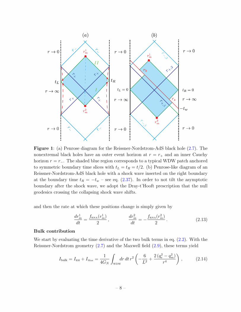
Figure 1: (a) Penrose diagram for the Reissner-Nordstrom-AdS black hole (2.7). The
nonextremal black holes have an outer event horizon at r = r+ and an inner Cauchy
horizon r = r−. The shaded blue region corresponds to a typical WDW patch anchored
to symmetric boundary time slices with tL = tR = t/2. (b) Penrose-like diagram of an
Reissner-Nordstrom-AdS black hole with a shock wave inserted on the right boundary
at the boundary time tR = −tw – see eq. (2.37). In order to not tilt the asymptotic
boundary after the shock wave, we adopt the Dray-t’Hooft prescription that the null
geodesics crossing the collapsing shock wave shifts.
and then the rate at which these positions change is simply given by
dr1m
dt=fRNA(r1
m)
2,
dr2m
dt= −fRNA(r2
m)
2. (2.13)
Bulk contribution
We start by evaluating the time derivative of the two bulk terms in eq. (2.2). With the
Reissner-Nordstrom geometry (2.7) and the Maxwell field (2.9), these terms yield
Ibulk = IEH + IMax =1
4GN
∫WDW
dr dt r2
(− 6
L2+
2 (q2e − q2
m)
r4
), (2.14)
– 8 –

where we have used the trace of Einstein equations: R = − 12L2 . Notice that in the
Maxwell contribution (i.e., the second term in the integrand), the electric and magnetic
charges appear with opposite signs! This fact is directly related to the vanishing of the
late time rate of complexity for magnetic black holes, as we will see below. Following [34,
42], the time derivative of the bulk action reduces to the difference of terms evaluated
at the future and past meeting points,
dIbulk
dt=
1
2GN
[r3
L2+q2e − q2
m
r
]r1m
r2m
. (2.15)
Joint contributions
As shown in figure 1(a), the WDW patch is cut off by a UV regulator surface at some
large r = rmax. However, the boundary contributions coming from this time-like surface
segment and the corresponding joints yield a fixed constant, i.e., they do not contribute
to the time derivative of the action. Further, with affinely-parametrized null normals
(for which κ = 0), the null surface term in eq. (2.3) vanishes. This leaves only the
joint terms at the meeting points, r = r1m and r2
m. The final result for these joint
contributions is given by [34]
Ijoint = − 1
2GN
[(r1m)2 log
[|fRNA(r1
m)|ξ2
]+ (r2
m)2 log
[|fRNA(r2
m)|ξ2
]], (2.16)
where ξ is the normalization constant appearing in the null normals, i.e., k · ∂t|r→∞ =
±ξ. In a moment, the addition of the counterterm (2.4) will eliminate the ξ dependence
of the action. Using eq. (2.12), the time derivative of eq. (2.16) becomes
dIjoint
dt= − 1
4GN
[2rfRNA(r) log
|fRNA(r)|ξ2
+ r2∂rfRNA(r)
]r1m
r2m
. (2.17)
Note that at late times, r1,2m approach the horizons and so the first term above vanishes.
Hence only the second term contributes to the late-time growth rate.
Counterterm contribution
The boundary counterterm (2.4) requires evaluating the expansion scalar Θ = ∂λ log√γ
in the null boundaries of the WDW patch and the final result is given by
Ict =r2
max
GN
[log
(4ξ2`2
ct
r2max
)+ 1
](2.18)
− (r1m)2
2GN
[log
(4ξ2`2
ct
(r1m)2
)+ 1
]− (r2
m)2
2GN
[log
(4ξ2`2
ct
(r2m)2
)+ 1
].
– 9 –

The term in the first line comes from the UV regulator surface and again only con-
tributes a fixed constant. Hence the time dependence comes only from the terms
evaluated at the meeting points in the second line. The time derivative of eq. (2.18)
has a compact form,
dIct
dt= −
[rfRNA(r)
2GN
log
(4ξ2`2
ct
r2
)]r1m
r2m
. (2.19)
Again at late times, this contribution vanishes and so it only changes the transientbehaviour in the growth rate at early times. It is useful to combine eqs. (2.17) and(2.1) to explicitly see that the ξ dependence is eliminated,
d
dt(Ijoint + Ict) = − 1
4GN
[2rfRNA(r) log
[|fRNA(r)|4`2ct
r2
]+ r2∂rfRNA(r)
]r1m
r2m
= − 1
4GN
[2rfRNA(r) log
[|fRNA(r)|4`2ct
r2
]+ 2
r3
L2− 2(q2
e + q2m)
r
]r1m
r2m
. (2.20)
Note that in contrast to eq. (2.15), the electric and magnetic charges contribute with
the same sign above.
Total growth rate
The growth rate of the holographic complexity (1.2) is then given by the sum of
eqs. (2.15) and (2.20), which yields
dCAdt
=1
π
d
dt(Ibulk + Ijoint + Ict) =
q2e
πGNr
∣∣∣∣r1m
r2m
− r fRNA(r)
2πGN
log
[|fRNA(r)|4`2
ct
r2
]r1m
r2m
. (2.21)
At late times, the past and future meeting points meet the outer and inner horizons,
respectively, and so the second term vanishes (since fRNA(r±) = 0). This leaves the
surprising result
limt→∞
dCAdt
=q2e
πGN r
∣∣∣∣r−r+
. (2.22)
Hence if we consider a purely magnetic black hole with qe = 0, the growth rate vanishes!
More generally, we might introduce
q2T ≡ q2
e + q2m and χ ≡ qe
qm, (2.23)
which allows us to re-express eq. (2.22) as
limt→∞
dCAdt
=χ2
1 + χ2
q2T
πGN r
∣∣∣∣r−r+
. (2.24)
– 10 –

0.0 0.5 1.0 1.5
-0.4
-0.2
0.0
0.2
0.4
0.6
Figure 2: The rate of change of complexity for the dyonic black hole given by eq. (2.7),
with r− = 0.3 r+, L = 0.5 r+ and `ct = L. We fix the parameters that determine the
geometry, but vary the ratio between electric and magnetic charges. As predicted
by eq. (2.22), when the charge is mostly magnetic, the growth rate of complexity
approaches zero at late times. The limit qm → 0 essentially matches the top curve for
χ = 10. Similarly the qe → 0 and the χ = 0.1 curves are indistinguishable on this scale.
Now fixing qT , which fixes the spacetime geometry (e.g., r±), this expression reveals a
nontrivial dependence of this growth rate on χ, the ratio of the electric and magnetic
charges. In particular, we see that as we put more of the charge qT into the magnetic
monopole with χ→ 0, the late-time growth rate shrinks to zero.
Figure 2 illustrates the full time-dependence of the growth rate, as we change the
ratio of the electric and magnetic charges while keeping the spacetime geometry fixed.
As expected from eq. (2.22), the rate approaches zero at late times when the black hole
is mostly magnetic.
2.2 Maxwell Boundary Term
The discussion in the previous section raises the question of whether there is a consistent
prescription for the holographic complexity that puts the electric and magnetic charges
on an equal footing? In the following, we will argue that such a prescription requires
that we modify the action with the addition of the Maxwell boundary term in eq. (2.5)
IµQ =γ
g2
∫∂M
dΣµ Fµν Aν . (2.25)
This surface term plays a natural role in black hole thermodynamics [94] — see [95, 96]
for a discussion in the context of the AdS/CFT correspondence. In particular, the
Euclidean version of the action I0 would yield the Gibbs free energy, associated with
– 11 –

the grand canonical ensemble where the temperature and chemical potential µ are held
fixed. Adding the boundary term (2.25) (with γ = 1) to the Euclidean action produces
the Legendre transform to the Helmholtz free energy, associated with the canonical
ensemble where the temperature and total (electric) charge Q are held fixed. This
boundary term was also shown to play a role in resolving the apparent tension between
electric-magnetic duality in four dimensions and the different partition functions of
electric and magnetic black holes [104–106] — see further discussion below.
As we noted above, adding this surface term (2.25) changes the boundary conditions
in the variational principle of the Maxwell field. Consider varying the Maxwell action
in eq. (2.2). Integrating by parts produces the equations of motion in the bulk but
leaves a boundary term proportional to δAµ,
δIMax =1
g2
∫Md4x√−g∇µF
µν δAν −1
g2
∫∂M
dΣµ Fµν δAν . (2.26)
Hence, a well-posed variational principle requires a Dirichlet boundary condition set-
ting δAa = 0 on the boundary (where the index a indicates that only the tangential
components of the potential are fixed). However, the latter can be modified by in-
troducing the surface term (2.25), in which case the variation produces the boundary
contribution
δIMax + δIµQ = · · · − 1
g2
∫∂M
dΣµ [(1− γ)F µν δAν + γ δF µν Aν ] . (2.27)
Of course, with γ = 1, the term proportional to δAν is eliminated and the required
boundary condition becomes nµ δFµa = 0, where nµ is a unit vector orthogonal to the
boundary ∂M. If we choose a gauge where n ·A = 0, we recognize this as the Neumann
boundary condition nµ ∂µ δAa = 0. With a general value of γ (and the same choice of
gauge), the potential would satisfy a mixed boundary condition,
γ nµ∂µδAa = (1− γ)Xab δAb , (2.28)
where the choice of Xab will depend on details of the problem of interest, e.g., [107–109].
Returning to the action (2.1), if we use the Maxwell equations ∇µFµν = 0, then
the boundary term (2.25) can be converted into a bulk term via Stokes’ theorem as
IµQ
∣∣on-shell
=γ
2g2
∫Md4x√−g FµνF µν , (2.29)
which is explicitly gauge invariant.2 Of course, the above expression takes the same
form as the bulk Maxwell action (2.2) and so we could just as well have re-expressed
2There is a subtlety here for the magnetic monopole contribution in that the boundary term must
be integrated over the boundary of all patches where the potential is well-defined — see appendix B.
– 12 –

the bulk action as a boundary term. In any event, combining eq. (2.29) with IMax yields
IMax + IµQ
∣∣on-shell
=2γ − 1
4g2
∫Md4x√−g FµνF µν . (2.30)
Hence in evaluating the WDW action for the general action Itot(γ), i.e., including the
contribution of the Maxwell boundary term in eq. (2.1), the only change that has to
be made to the previous calculation is to change the overall coefficient of the Maxwell
contribution in eq. (2.14). As a result, eq. (2.15) is replaced by
d
dt(Ibulk + IµQ) =
1
2GN
[r3
L2− (2γ − 1)
q2e − q2
m
r
]r1m
r2m
. (2.31)
Subsequently, the final result for the late-time growth rate for the complexity be-
comes
limt→∞
dCAdt
=(1− γ) q2
e + γ q2m
πGNr
∣∣∣∣r−r+
=(1− γ)χ2 + γ
1 + χ2
q2T
πGNr
∣∣∣∣r−r+
. (2.32)
Therefore if we set γ = 1, the dependence on the electric charge drops out of the
numerator and the late-time growth rate is primarily sensitive to the magnetic charge.
In particular then, with this choice of γ, the late-time growth rate drops to zero for an
electrically charged black hole at late times.
The above discussion shows us that the growth rate (or more generally the on-shell
action) is symmetric under electric-magnetic duality, i.e., Fµν ↔ Fµν = 12εµνρσF
ρσ, if
at the same time we exchange the action3
Itot(γ)↔ Itot(1− γ) , (2.33)
i.e., we modify the coefficient of the Maxwell boundary term (2.25) as indicated above.
Then γ = 1/2 is singled out as the special choice which leaves the action unchanged
in eq. (2.33). Of course, looking back at eq. (2.30), we see that the combination of
the bulk and boundary terms for the Maxwell field vanishes on-shell. However, the
complexity is still sensitive to the electromagnetic field through its back-reaction on
the geometry. In particular, the holographic complexity only depends on the duality
invariant combination q2T = q2
e + q2m, as appears in the metric (2.7). For example,
eq. (2.32) becomes
limt→∞
dCAdt
∣∣∣∣γ=1/2
=q2e + q2
m
2πGN r
∣∣∣∣r−r+
, (2.34)
and as desired, the electric and magnetic charges influence the complexity growth rate
on an equal footing. However, as we discuss in section 5, this expression produces a
puzzle in the limit of zero charges.
3This equivalence was noted by [106] for γ = 1.
– 13 –

Of course, the reader may wonder why we should expect that that magnetic and
electric black holes should compute at the same rate. First, let us recall the expectation
that the late-time growth of the complexity should be given by eq. (1.3), i.e., dC/dt ∼ST , but both the entropy S and temperature T are governed by the spacetime geometry,
as given in eq. (2.8). Hence it is natural to think that this rate should be controlled
by q2T = q2
e + q2m, the combination appearing in the metric (2.7). This conclusion can
also be motivated by the shock wave geometries, which we study in the next section.
In this context, both electric or magnetic black holes exhibit the same back-reaction
and hence it is natural to think that the holographic complexity should respond in the
same manner independent of the nature of the charge.
2.3 Shock Wave Geometries
Another property that holographic complexity should exhibit is the switchback effect,
which is related to the complexity of precursor operators [18, 32] — see further dis-
cussion in section 5. We will follow closely the analysis and notation of [40, 41]. To
examine this feature, we consider a Vaidya geometry where a(n infinitely) thin shell of
null fluid collapses into a charged black hole. If the shell only injects a small amount of
energy into the system, then the black hole’s event horizon shifts by a small amount,
i.e.,r+,2
r+,1
= 1 + ε , (2.35)
where the subscripts 1 and 2 indicate before and after the shock wave, respectively.
The scrambling time associated with this perturbation is then given by
t∗scr =1
2πT1
log2
ε. (2.36)
For the chaotic dual of the black hole, the switchback effect then predicts that for
any time t after the perturbation is introduced, the complexity remains essentially
unchanged for t < t∗scr but then the difference of complexities (for the perturbed and
unperturbed states) begins to grow linearly afterwards, i.e., t > t∗scr. Our goal here is to
investigate to what extent the CA proposal reproduces this behaviour for the charged
black holes discussed in the previous sections.
Charged shock wave geometry
Figure 1(b) illustrates the spacetime geometry for a shock wave collapsing into a
Reissner-Nordstrom black hole from the right boundary at t = −tw. Note that fol-
lowing [40, 41], we adopt the Dray-‘t Hooft prescription that the null geodesics shift
– 14 –

upon crossing the collapsing shock wave. For simplicity, we assume that the thin shell
is neutral, i.e., it carries energy but no charges. The corresponding metric is
ds2 = −F (r, v) dv2 + 2 dr dv + r2 (dθ2 + sin2 θdφ2)
with F (r, v) =r2
L2+ 1− f1(v)
r+q2e + q2
m
r2(2.37)
where
fs(v) = ω1 (1−H(v − vs)) + ω2H(v − vs) .
(with H(v) denoting the usual Heaviside function). Before and after v = vs, the metric
has precisely the form given in eq. (2.7) with ω = ω1 and ω2, respectively. However,
we must evaluate the tortoise coordinate (2.10) for each region and then following
eq. (2.11), define the time coordinate as t = v − r∗(r). Note that taking the limit
r →∞, we find vs = −tw on the boundary.
The geometry of the WDW patch is characterized by a number of dynamical points:
r1m and r2
m, the meeting points of the future and past null boundaries, respectively; and
rs and rb, the point where the null shell crosses the past right and future left boundaries,
respectively. These positions are determined by the boundary times with
tR + tw = −2r∗2(rs) ,
tL − tw = 2r∗1(rs)− 2r∗1(r2m) ,
tL − tw = 2r∗1(rb) ,
tR + tw = 2r∗2(r1m)− 2r∗2(rb) . (2.38)
In the following, it is sufficient to restrict our attention to the case tL = tR = 0 and to
study the behaviour resulting from pushing the perturbation to earlier times t = −tw.
Let us note that with these choices, eq. (2.38) yields a simple result for the dynamical
points in the limit of large tw, namely,
limtwT→∞
rs = r+,2 limtwT→∞
r2m = r−,1
limtwT→∞
rb = r+,1 limtwT→∞
r1m = r−,2 . (2.39)
Results for Switchback Effect
Following [41], the switchback effect is revealed (or not) in the ‘complexity of formation’
comparing the holographic complexity of the above shockwave geometry with that of
the static black hole (2.7) with ω = ω1 (and the same charges). We begin by considering
the CA proposal for the action without the Maxwell boundary term (2.5), i.e., we again
set γ = 0 in eq. (2.1) as in section 2.1. The details of our calculations are given in
– 15 –

0 1 2 3 40.0
0.5
1.0
1.5
2.0
2.5
Figure 3: The difference of complexities of formation in the shock wave geometry as
a function of the insertion time tw, for a light shock wave r+,2 = (1 + 10−6)r+,1 and
parameters L = 0.5 r+,2, r−,1 = 0.5 r+,2 and `ct = L (r−,2 is then fixed by the condition
that qT is the same after the shock wave). The dashed vertical line is the scrambling
time for the shock wave with these geometric parameters. We investigate the effect of
varying the ratio between electric and magnetic charges: after the scrambling time, the
complexity essentially remains constant for the solution with mostly magnetic charges,
as predicted by eq. (2.40).
appendix A. In figure 3, we present the difference of complexities for a light shock wave
producing r+,2 = (1+10−6)r+,1 (i.e., ε = 10−6 in eq. (2.35)). Notice that the complexity
remains unchanged by the perturbation up until tw = t∗scr but afterwards, the difference
quickly makes a transition to linear growth.4 Several curves are shown in the figure
where the geometry is held fixed (i.e., q2T = q2
e + q2m is fixed) but the ratio χ = qe/qm
is varied. We see that the rate of the linear growth tw ≥ t∗scr decreases to zero as more
of the charge is put into the magnetic monopole, i.e., as χ→ 0. Hence the switchback
effect vanishes (with this choice of γ) for a black hole with pure magnetic charge. This
result might be expected since there is a close connection between the late-time rate of
growth of the complexity in the static black hole and dCA/dtw, as discussed in [41].5
4For heavier shock waves, e.g., ε ∼ 10−1, the initial regime over which the complexity is constant
essentially disappears, similar to the behaviour found for neutral black holes in [41].5Comparing eq. (2.24) with the result in eq. (2.40) for tw > t∗scr, we see that dCA/dtw '
2 dCA/dt|t→∞, as predicted by [41].
– 16 –

The rate dCA/dtw can be evaluated analytically to find (see appendix A)
dCAdtw' O
(χ2
1 + χ2εe2πT1tw
)for tw < t∗scr ,
dCAdtw' χ2
1 + χ2
q2T
πGN
(1
r
∣∣∣∣r−,1r+,1
+1
r
∣∣∣∣r−,2r+,2
)for tw > t∗scr . (2.40)
Hence as for the growth rate of the eternal black hole case in section 2.1, the complexity
rate after the scrambling time depends on the ratio between electric and magnetic
charges and in particular, dCA/dtw vanishes as χ→ 0.
We can confirm the scaling with χ in eq. (2.40) by simply multiplying the curves
in figure 3 by the factor (1 +χ2)/χ2 and then we see in figure 4(a) that essentially they
all collapse onto a single curve. The only exception is for the smallest ratio, χ = 0.1,
which is slightly shifted to the right. This behaviour arises because for smaller χ, there
is a greater sensitivity to the scale `ct in the null counterterm (2.4). The dependence
on this ambiguity in the definition of the WDW action is illustrated in figure 4(b). We
note, however, that this ambiguity does not effect the final rate dCA/dtw but only the
transition between the two regimes in eq. (2.40).
Further, eq. (2.40) suggests a regime of exponential growth for tw < t∗scr. However,
this regime actually becomes smaller as the black hole becomes mostly magnetic, i.e.,
as χ becomes small, as illustrated in figure 5. For the mostly electric black hole (with
χ = 10), we see a good agreement with an exponentially growing mode with the
Lyapunov exponent λL = 2πT until times of the order of the scrambling time. For
the mostly magnetic black hole (with χ = 0.015), the amplitude of the exponential
mode is suppressed by a factor of χ2, which shifts the corresponding curve down in the
figure. In addition, we see that the exponentially growing mode is only the dominant
contribution at earlier times. This reflects the fact that the analysis producing the
tw < t∗scr expression in eq. (2.40) really only applies for χ & 1 — see appendix A. When
this exponential mode is suppressed by small χ, it must compete with other transient
dynamics (e.g., depending on `ct) and therefore, its role becomes less important in
this regime. In particular, if the black hole is purely magnetic (with χ = 0), the
exponentially growing mode is absent.
Of course, the above results (with γ = 0) are modified if we include the Maxwell
boundary term (2.5). In particular, eq. (2.40) is replaced by
dCAdtw' O
((1− γ)χ2 + γ
1 + χ2εe2πT1tw
)for tw < t∗scr ,
dCAdtw' (1− γ)χ2 + γ
1 + χ2
q2T
πGN
(1
r
∣∣∣∣r−,1r+,1
+1
r
∣∣∣∣r−,2r+,2
)for tw > t∗scr . (2.41)
– 17 –

0 1 2 3 4
0
1
2
3
4
5
6
(a)
0 1 2 3 4
0
2
4
6
(b)
Figure 4: (a) The complexity for the shock wave geometry as a function of the insertion
time tw, for a light shock wave r+,2 = (1 + 10−6)r+,1 and parameters L = 0.5 r+,2,
r−,1 = 0.5 r+,2 and `ct = L. (Further, r−,2 is determined by fixing qT to be the same
before and after the shock wave.) We show the result for rescaling the curves in figure3
by the factor (1 + χ2)/χ2. We essentially see that the curves lie on top of each other,
except the for smallest χ, as it is more sensitive to the transient behaviour controlled
by `ct. (b) The influence of the transient behaviour for the complexity in the shock
wave geometry. We show in solid χ = 0.1 and in dot-dashed χ = 10 to contrast the
effect of varying `ct. For `ct = 0.1L, both curves are essentially on top of each other,
but for `ct ∼ L, the curves with small χ are more sensitive to this ambiguous scale.
Hence if we choose γ = 1, the roles of the magnetic and electric charges are reversed.
For example, with this choice, black holes with magnetic charges exhibit the desired
switchback effect while those with a purely electric charge would not. Further, similar
to the discussion in section 2.2, if we choose γ = 1/2, the χ dependence drops out of
eq. (2.41) and the behaviour only depends on q2T = q2
e +q2m. Therefore, with this choice,
both electric and magnetic black holes exhibit the same switchback effect.
As a final comment here, let us note that for a light shock wave, r±,2 ' r±,1 and
the two contributions in eq. (2.41) for the rate at large tw are essentially the same.
Further, this rate is essentially twice the late-time growth rate in eq. (2.32).6 In fact,
as discussed in [41], there is a more general relationship that extends to heavy shocks,
i.e.,dCAdtw
=dCAdtR− dCAdtL
, (2.42)
because of the symmetry of the shock wave geometry under
tR → tR −∆t , tL → tL + ∆t , tw → tw + ∆t . (2.43)
6Of course, there is a similar relationship between the rates in eqs. (2.40) and (2.24) for γ = 0.
– 18 –

0.0 0.5 1.0 1.5 2.0 2.5-30
-25
-20
-15
-10
-5
0
5
Figure 5: The exponential growth for the complexity with a light shock wave, such
that r+,2 = (1 + 10−6)r+,1, and also with L = 0.5r+,2, r−,1 = 0.5r+,2, lct = L. We show
two examples, one for a black hole with mostly electric charge χ = 10 and one with
mostly magnetic charge χ = 0.015. For the larger χ, the dynamics is well approximated
by an exponentially growing mode with Lyapunov exponent λL = 2πT until times of
the order of the scrambling time (vertical black line), as in eq. (2.40). For the smaller
value of χ, the amplitude of this initial mode is suppressed both by the energy of the
shock wave and by a factor of χ2. The exponentially growing mode only dominates
at very early times because it must compete with other transient effects. In the limit
that the black hole has only magnetic charges (i.e., χ = 0), this exponentially growing
mode is absent.
Hence for large tw, dCA/dtw is related to the late-time growth rates of the complexity on
either side of the shock wave.7 Therefore, we can anticipate that the switchback effect
will be absent in exactly the same situations where the late-time growth rate vanishes,
e.g., for magnetic black holes with γ = 0. Of course, this is precisely the behaviour
found in this subsection.
7That is, given a large tw = t0, we use eq. (2.43) to shift (tR, tL, tw) = (0, 0, t0) → (t0,−t0, 0).
Then the right-hand side of eq. (2.42) has a contribution corresponding to the growth rate on the
right boundary at very late times and another coming from very early times on the left boundary. In
fact, the latter is probing the white hole part of the Penrose diagram when the complexity is actually
decreasing, e.g., [23]. However, by the time symmetry of the unperturbed Penrose diagram, this
early-time rate matches the late-time rate up to an overall sign, i.e., the minus sign in eq. (2.42).
– 19 –

3 Charged Dilatonic Black Hole
In this section, we investigate the CA proposal (1.2) in a broader class of charged black
holes. This investigation is motivated by the question of understanding to what extent
our results in the previous section are special to the precise couplings of the Einstein-
Maxwell theory. In particular, in many string theoretic settings, the gauge field will
also be coupled to various moduli or scalars, e.g., see [110, 111]. The presence of these
new couplings lead to scalar hair on the charged black holes, and may change the nature
of the spacetime singularities and the casual structure of the corresponding black holes.
Hence we would like to understand if these changes to the spacetime geometry modify
the behaviour of the holographic complexity in an essential way.
In the following, we consider a simple extension of the Einstein-Maxwell theory,
where Maxwell field has an “exponential coupling” to an additional scalar field, the
so-called dilaton. The corresponding charged dilatonic black holes were introduced for
asymptotically flat geometries in [112, 113] and they were extended to asymptotically
AdS geometries in [114–116]. The AdS solutions were further explored in, e.g., [117–
120]. Holographic complexity of dilatonic black holes has been previously studied for
several models [30, 36, 38, 39]. Our investigation of the holographic complexity for
these dilatonic black holes will show that the vanishing of the late-time growth rate
found in the previous section (for certain choices of charges and boundary terms) is
not a generic result for charged black holes. Rather, for the theories studied here, the
analog of the Maxwell boundary term modifies the complexity growth rate but the
coefficient can not be chosen to reduce the rate to zero generally. However, we will
see that the latter can still be accomplished in the theories where the charged black
holes have the same causal structure as the Reissner-Nordstrom black holes. Hence
our conclusion is that the causal structure of the spacetime geometry is the essential
feature leading to the vanishing late-time growth rate in the previous section.
As commented above, we will be studying holographic complexity in a theory where
gravity couples to a dilaton, as well as the Maxwell field (and cosmological constant),
Ibulk =1
16πGN
∫Md4x√−g(R− 2(∂φ)2 − V (φ)
)− 1
4g2
∫Md4x√−ge−2αφFµνF
µν
(3.1)
where the dilaton potential V (φ) given by
V (φ) = − 2
(1 + α2)2L2
[α2(3α2 − 1)e−2φ/α + (3− α2)e2αφ + 8α2e(α−1/α)φ
]. (3.2)
The total action takes the form
Itot = Ibulk + Isurf + Ict , (3.3)
– 20 –

where the gravitational boundary terms, Isurf and Ict, are the same as in eqs. (2.3)
and (2.4), respectively. In subsection 3.2, we will also consider the effect of adding
the analog of the Maxwell surface term (2.5), as well as a new boundary term for the
dilaton. Here, we are again focusing on the case of four bulk dimensions for simplicity.
The parameter α controls the strength of the coupling of the dilaton to the Maxwell
field, but it also determines the shape of the potential in eq. (3.2). The latter is tuned
so that φ = 0 is a critical point (i.e., a local maximum) with V (0) = −6/L2, where L
is the curvature scale of the corresponding AdS vacuum. We also note that the global
shape of the potential depends on the value of α, namely,
• For 0 < α2 < 1/3, as well as the maximum at φ = 0, V (φ) has a minimum at
φ = − α1+α2 log
(1−3α2
3−α2
). Moreover, limαφ→±∞ V (φ) = ∓∞.
• For 1/3 < α2 < 3, V (φ) has only the global maximum at φ = 0. In this case,
limφ→±∞ V (φ) = −∞.
• For α2 > 3, V (φ) has the maximum at φ = 0 and a minimum at φ = α1+α2 log
(3α2−1α2−3
).
Asymptotically, we find limαφ→±∞ V (φ) = ±∞.
• For the special values α2 = 1/3 , 1 and 3, V (φ) has only a maximum at φ = 0,
but it is symmetric under φ → −φ. More generally, the potential is invariant
with the following substitutions: φ→ −φ and α→ 1/α.
Of course, if we set α = 0, the dilaton decouples from the Maxwell field and the potential
(3.2) reduces to a simple cosmological constant, i.e., V (φ)|α=0 = −6/L2. Hence in this
limit, the theory (3.1) reduces to the Einstein-Maxwell theory (2.2) from the previous
section coupled to an additional massless scalar field.
For this theory (3.1), a class of static spherically-symmetric solutions describing
electrically charged dilaton black holes is given by [114]
ds2 = −f(r) dt2 +dr2
f(r)+ U2(r) (dθ2 + sin2 θ dφ2) , (3.4)
F =g√
4πGN
qe e2αφ
U(r)2dr ∧ dt , eαφ =
U(r)
r,
with
f(r) =(
1− c
r
)(1− b
r
) 1−α2
1+α2
+U2(r)
L2, (3.5)
U2(r) = r2
(1− b
r
) 2α2
1+α2
, q2e =
c b
1 + α2,
– 21 –

where c and b are integration constants. We note that this solution interpolates between
the Reissner-Nordstrom black hole (α → 0) and Schwarzschild (α → ∞).8 Moreover,
if we set b = 0, the solution reduces to the (uncharged) Schwarzschild-AdS solution
independently of the value of α.
Implicitly, for the following, we will only consider nonextremal solutions, with b
positive and c sufficiently large, e.g., c� b. The causal structure for these solutions is
illustrated in figure 6. The geometry has a curvature singularity at r = b where U(r)
vanishes with any finite α. In general, there are horizons determined by f(r±) = 0.
However, for α2 ≥ 1/3, one generally finds a single (real) solution r+ > b and the
singularity is spacelike. Hence in examining the CA proposal, we will find the future
null boundaries of the WDW patch meet the singularity (at late times), as illustrated
in the left panel of figure 6. Furthermore, for 0 < α2 < 1/3, there is an additional inner
horizon at r− between the event horizon and the singularity at r = b, i.e., b < r− < r+,
as shown in the right panel of figure.9
Following [119], the mass of the black hole (3.4) can be shown to be
M =1
2GN
(c+
1− α2
1 + α2b
)(3.6)
It is useful to use f(r+) = 0 to rewrite the parameter c in terms of the position of the
event horizon of the black hole,
c = r+ +r3
+
L2
(1− b
r+
)(3α2−1)/(1+α2)
. (3.7)
Then the temperature and entropy of the black hole can be expressed as
T =1
4π
∂f
∂r
∣∣∣∣r=r+
=1
4πr+
(1− b
r+
)(1−α2)/(1+α2)
+3r+(1 + α2)− 4b
4πL2(1 + α2)
(1− b
r+
)(α2−1)/(1+α2)
,
S =πU2(r+)
GN
=π
GN
r2+
(1− b
r+
)2α2/(1+α2)
. (3.8)
8In the latter case, the coordinate transformation r → r+ b yields the usual coordinate system for
the Schwarzschild-AdS metric.9Of course, just as for the Reissner-Nordstrom-AdS solution, there is a threshold beyond which the
charged dilatonic solution (3.4) becomes a naked singularity, e.g., if we begin with large c but then
reduce its value while holding b fixed. For the theories with 0 < α2 < 1/3, the threshold corresponds to
the point where r− coincides with r+, and hence the solution becomes an extremal black hole (matching
the behaviour of the Reissner-Nordstrom-AdS black holes). However, the situation is different for
α2 ≥ 1/3 where the nonextremal black holes only have a single horizon. In this case, the threshold is
reached when the event horizon meets the singularity, i.e., r+ → b, and hence the threshold solution
contains a null singularity.
– 22 –

Figure 6: Causal structure for the charged dilatonic black hole given by eq. (3.4). The
left panel corresponds to α2 ≥ 1/3, for which the causal structure is similar to that
of the Schwarzschild-AdS black hole, with a spacelike singularity at r = b. The right
panel corresponds to 0 ≤ α2 < 1/3, for which the causal structure is similar to that
of the Reissner-Nordstrom-AdS black hole and the timelike singularity lies behind an
inner Cauchy horizon (at r = r−).
It would be interesting to study which black hole solutions are thermodynamically and
dynamically stable (e.g., in analogy to refs. [95, 96], however, we do not pursue this
question here).
3.1 Complexity Growth
We will now study the time-dependence of the holographic complexity of the charged
dilatonic black holes presented above using the CA proposal. Of course, in contrast to
the previous discussion of the dyonic Reissner-Nordstrom-AdS black holes in section
2, we only have the solutions carrying purely electric charges here. We will follow the
discussion in [34], which is straightforward to adapt to these solutions. Further, we
will only be considering the action (3.3) here and defer the discussion of additional
boundary terms to the next sections. Since we are primarily interested in the late-time
– 23 –

growth rate, for the theories with α2 ≥ 1/3, we will assume that the WDW patch has
already lifted off of the past singularity in the following calculations, as illustrated in
left panel of figure 6.
Bulk Contribution
Evaluating the bulk action (3.1) yields
Ibulk =1
2GN
∫WDW
dtdr
[− r2
(1 + α2)2L2
(8α2
(1− b
r
) 3α2−1
α2+1
+ (3− α2)
(1− b
r
) 4α2
α2+1
+ α2(3α2 − 1)
(1− b
r
)2α2−1
α2+1)
+q2e
r2
], (3.9)
The time derivative then becomes
dIbulk
dt=
1
2GN
q2e
r+
r2
L2(1 + α2)
(r(1 + α2)− b
)(1− b
r
) 3α2−1
1+α2
r1m
r2m
. (3.10)
For black holes with just one horizon, i.e., α2 ≥ 1/3, r1m corresponds to the position
of the singularity, that is r1m = b. On the other hand, for 0 < α2 < 1/3, the past
meeting point approaches the Cauchy horizon at late times, i.e., r1m → r− – see figure
6. Similarly, at late times, r2m → r+ for all α.
GHY contribution
As noted above, for 0 < α2 < 1/3, the future tip of the WDW patch is the joint where
the future null boundaries meet (with r− < r1m < r+). In contrast for α2 ≥ 1/3, the
WDW patch ends on the spacelike singularity at r = b and so as usual, we introduce a
regulator surface at r = b + ε0. We must evaluate the Gibbons-Hawking-York (GHY)
term, given in eq. (2.3), on this surface and consider the limit ε0 → 0. The trace of the
extrinsic curvature of the regulator surface is given by
K = − 1
2√−f(r)
(∂rf(r) + 2
∂r(U(r)2)
U(r)2f(r)
) ∣∣∣∣r=b+ε0
. (3.11)
However, notice that in integrating this term over the surface, the spherical measure is
not r2, e.g., as in the Schwarzschild-AdS solution, but U(r)2 instead. Hence the GHY
contribution from the regulator surface becomes
IGHY = −U(r)2
2GN
(∂rf(r) + 2
∂r(U(r)2)
U(r)2f(r)
)(t
2+ r∗∞ − r∗(r)
) ∣∣∣∣r=b+ε0
. (3.12)
– 24 –

Now taking time derivative and the limit ε0 → 0 yields
dIGHY
dt=
38GN
(c− b− b3
L2
)for α2 = 1
3
(1+3α2)4GN (1+α2)
(c− b) for α2 > 13
(3.13)
Notice that subtleties in the ε0 → 0 limit produce the extra term proportional to b3
here when we have precisely α2 = 1/3.
Joint contributions
If we focus on α2 < 1/3, the only joints which contribute to the time dependence are
those at the future and past meeting points, i.e., r = r1m and r2
m – see figure 6. The
corresponding joint contributions are given by
Ijoint(r1m) + Ijoint(r
2m) = −U
2(r1m)
2GN
log|f(r1
m)|ξ2
− U2(r2m)
2GN
log|f(r2
m)|ξ2
. (3.14)
The time derivative then yields
d
dt
(Ijoint(r
1m) + Ijoint(r
2m))
=
[U2(r)
4GN
(∂rf(r) +
∂r(U2(r))
U2(r)f(r) log
|f(r)|ξ2
)]r2m
r1m
(3.15)
As discussed above for α2 ≥ 1/3, the future boundary of the WDW patch is the
regulator surface just above the spacelike singularity. While there are joints where the
future null boundaries meet this surface, their size is proportional to U2(r = b + ε0)
which vanishes in the limit ε0 → 0. Hence the corresponding joint contributions vanish.
Therefore in this case, the contribution to the time derivative comes from the past
meeting point and it is precisely given by the expression above evaluated at r = r2m.
Counterterm contribution
To evaluate the surface counterterm (2.4), we begin by choosing the affine parameter
along the null boundaries as
λ =r
ξ, (3.16)
which then yields
Θ =ξ∂r(U(r)2)
U(r)2. (3.17)
The sum of the counterterm contributions on the four null boundaries then reads
Ict =1
GN
∫ rmax
r1m
dr ∂r(U(r)2) logξ`ct∂r(U(r)2)
U(r)2+
1
GN
∫ rmax
r2m
dr ∂r(U(r)2) logξ`ct∂r(U(r)2)
U(r)2.
(3.18)
– 25 –

This integration is nontrivial for general values of α. However, the time dependence
has a simple form,
dIctdt
=1
2GN
[∂r(U(r)2)f(r) log
ξ`ct∂r(U(r)2)
U(r)2
]r2m
r1m
. (3.19)
Implicitly, the contribution evaluated at r1m would absent at late times if we consider the
solutions for α2 ≥ 1/3. As expected, when eqs. (3.15) and (3.19) are added together,
the combined contribution to the time derivative is independent of ξ.
Total growth rate
Now we combine all of the contributions in eqs. (3.10), (3.13), (3.15) and (3.19) and
consider the late-time limit, to find
limt→∞
dCAdt
=
q2e
πGN
[1r−− 1
r+
]for α2 < 1
3
1π
[2M − q2
e
GNr+− 3b
4GN− b3
4GNL2
]for α2 = 1
3
1π
[2M − q2
e
GNr+− b
(1+α2)GN
]for α2 > 1
3
(3.20)
Of course, the late-time growth rate depends on the causal structure of the black hole
– see figure 6. In particular, we note that in the theories with 0 ≤ α2 < 1/3 for
which the causal structure matches that of the Reissner-Nordstrom-AdS black holes,
the form of the late-time rate above has precisely the same form as in eq. (2.22) for
the latter solutions. In fact, the result in eq. (3.20) reduces to precisely the growth
rate of the (electrically charged) Reissner-Nordstrom-AdS black holes when α → 0.
We also note that in the limit α → ∞, we recover the late-time growth rate of the
Schwarzschild-AdS solution, i.e., dCA/dt = 2M/π. Further, we observe that using (3.7),
this rate will vanish as we approach extremality, i.e., as r+ → r− for 0 ≤ α2 < 1/3,
which again parallels the behaviour of the (electrically charged) Reissner-Nordstrom-
AdS black holes [34, 55]. We also note that for the α2 ≥ 1/3 solutions, the rate vanishes
in the limit r+ → b, where the black holes become null singularities.
As an example, we show in figure 7 the full time evolution of complexity for α2 =
1/2, for which the causal structure resembles that of an Schwarzschild-AdS black hole
(left panel in figure 6). The behaviour is very similar to that of the latter neutral
black holes, as shown in the detailed analysis of [34]. Up to a certain critical time,
the WDW patch ends on both the past and future singularities, and during this time,
the complexity remains constant. After this critical time, the past null boundaries
meet at r = r2m, as discussed above, and at late times, this joint approaches the event
horizon. In this period of time, rate of change of the complexity exhibits a transient
– 26 –

0.0 0.5 1.0 1.5 2.0 2.5
-2.5
-2.0
-1.5
-1.0
-0.5
0.0
0.5
1.0
Figure 7: The time dependence of complexity for an electrically charged Maxwell-
Dilaton black hole (without the addition of the Maxwell boundary term). We evaluate
for concreteness α = 1/√
2, which corresponds to a black hole with a causal structure
that resembles that of an Schwarzschild-AdS black hole. The parameters are chosen to
be `ct = L, L = 0.9, b = 0.75 and c = 2.5. In analogy to the Schwarzschild-AdS black
hole, the complexity does not change until a certain critical time, where the WDW
patch leaves the past singularity. Then, the complexity approaches the late time limit
from above, with a transient dependence on `ct, at times of the order of the inverse
temperature.
behaviour (which depends on the counterterm scale `ct) and then by a time of the order
of the inverse temperature, it has overshot the late-time limit which it subsequently
approaches from above.
3.2 Boundary Terms
Next we examine how the growth rate of the holographic complexity (1.2) for the
charged dilatonic black holes (3.4) is effected by the addition of two boundary terms,
involving the Maxwell and dilaton fields.
– 27 –

Maxwell Boundary Term
We begin with the Maxwell boundary term for the new theory (3.1),
IµQ =γαg2
∫∂M
dΣµ Fµν Aν e
−2αφ , (3.21)
where γα is a free parameter. Following the same reasoning as in section 2.2, this
boundary term changes the boundary condition imposed on the Maxwell field in the
variational principle. However, we should add that implicitly we would also be assuming
a Dirichlet boundary condition for the dilaton, i.e., δφ|∂M = 0. Further in analogy
with (2.29), if the Maxwell field satisfies the equation of motion ∇µ(e−2αφF µν) = 0,
this boundary term is equivalent to
IµQ
∣∣on shell
=γα2g2
∫Md4x√−g e−2αφ F µνFµν . (3.22)
Hence, it is straightforward to evaluate the effect of this boundary term (3.21) on the
time dependence of the WDW action and one finds
dIµQ
dt= −γα q
2e
GN
[1
r2m
− 1
r1m
](3.23)
Of course, all of the contributions calculated previously are unchanged. Hence adding
in the above expression, the late time limits in eq. (3.20) are now replaced by
limt→∞
dCAdt
=
(1−γα)q2
e
πGN
[1r−− 1
r+
]for α2 < 1
3
1π
[2M − (1−γα)q2
e
GNr+− 3(b+γαc)
4GN− b3
4GNL2
]for α2 = 1
3
1π
[2M − (1−γα)q2
e
GNr+− b+γαc
(1+α2)GN
]for α2 > 1
3
(3.24)
Notice that, if we fix γα, the limits α → ∞ and α → 0 discussed below eq. (3.20)
are unchanged, i.e., they yield the late-time growth rates of the Schwarzschild-AdS
and electrically charged Reissner-Nordstrom-AdS black holes, respectively. Further, as
before, the above rate will vanish as we approach extremality for 0 ≤ α2 < 1/3, and as
we approach the limit of a null singularity for α2 ≥ 1/3.
One interesting choice to consider for the boundary coefficient is γα = 1, for which
eq. (3.24) becomes
limt→∞
dCAdt
∣∣∣∣γα=1
=
0 for α2 < 1
3
12π
[M − 3b
4GN− b3
2GNL2
]for α2 = 1
3
1π
[2α2
1+α2
(M − b
(1+α2)GN
)]for α2 > 1
3
(3.25)
– 28 –

That is, for 0 ≤ α2 < 13
in which case the causal structure matches that of the Reissner-
Nordstrom-AdS black holes, the (electrically) charged dilatonic black holes fail to com-
plexify at late times. This precisely matches the behaviour found in section 2.2. On the
other hand, for α2 > 13
in which case the causal structure is similar to the Schwarzschild-
AdS black holes, the late-time growth rate remains nonvanishing. However, we observe
that in the uncharged limit (i.e., b→ 0), eq. (3.25) does not yield the expected growth
rate of 2M/π – see section 5 for further discussion.
Dilaton Boundary term
Next we consider the following boundary term for the dilaton
Iφ =γφ
4πGN
∫∂M
dΣµ φ ∂µφ . (3.26)
As for the Maxwell boundary term (3.21) (or eq. (2.25) in the previous section), this
term modifies the character of the boundary condition which must be imposed on
the dilaton in the variational principle. For example, while γφ = 0 corresponds to
a Dirichlet boundary condition (i.e., δφ|∂M = 0), setting γφ = 1 yields a Neumann
boundary condition (i.e., nµ∂µδφ|∂M = 0). More general choices of this parameter lead
to mixed boundary conditions. Further, if both γφ and γα are nonvanishing, the dilaton
will have a more complicated boundary condition involving terms proportional to the
integrand in eq. (3.21).
Let us first consider black holes for 0 < α2 < 1/3, in which the causal structure
resembles the Reissner-Nordstrom-AdS black hole as shown in figure 6. In this case, the
boundary term lives only on the null boundaries of the WDW patch but in this case,
the derivative appearing in eq. (3.26) is actually tangent to the boundary. Therefore
the boundary term reduces to an integral over the joints where the null boundaries
intersect, namely
Iφ =γφ
8πGN
∫Σ′d2x√σφ2 , (3.27)
where each joint term carries a sign according to the conventions of [26]. However, one
finds in this case
limt→∞
dIφdt
= 0 . (3.28)
Hence, adding the dilaton boundary term (3.26) does not change the complexity growth
rate at late times for these black holes. Nevertheless, the transient behaviour of the
holographic complexity at early times will be modified by this term, but we will not
explore this here.
Next, we turn to the case α2 ≥ 1/3, in which the causal structure resembles the
Schwarzschild-AdS black hole. In this case, the contribution from the null boundaries
– 29 –

of the WDW patch still reduce to contributions on various joints, which again do not
contribute to the late-time growth rate. However, there is an additional contribution
coming from the (spacelike) regulator surface at the future singularity – see figure 6.
Evaluating eq. (3.26) on this boundary and considering the late time limit, we find
limt→∞
dIφdt
= limε0→0
γφU(r)2f(r)φ ∂rφ
2GN
∣∣∣∣r=b+ε0
. (3.29)
Unfortunately, for γφ 6= 0, this expression is divergent. Therefore adding the dilaton
boundary term (3.26) spoils the good behaviour of the regularization procedure at the
singularity. Therefore, we do not consider these boundary terms further here.
Hence, our general results for the late-time growth rate of the holographic com-
plexity including the Maxwell boundary term (3.21) are summarized eq. (3.24) for the
electrically charged black holes. Of course, these results match the growth rates with-
out the Maxwell boundary term in eq. (3.20) when we set γα = 0. However, when the
Maxwell boundary term (3.21) was included, we also showed in eq. (3.25) that choosing
γα = 1 sets the late-time growth rate to zero for the cases where the causal structure
was like that of the Reissner-Nordstrom-AdS black holes, i.e., for α2 < 1/3. No such
choice was possible when the causal structure had the form of the Schwarzschild-AdS
black holes, i.e., for α2 ≥ 1/3. The former behaviour was analogous to that found
in the Einstein-Maxwell theory in section 2 and therefore it appears that the causal
structure of the black hole was one of the essential features producing the unusual
behaviour found there. However, we note that our analysis here focused only on elec-
trically charged black holes and we did not consider dyonic or magnetically charged
black holes. Unfortunately the latter solutions are not yet known for the Einstein-
Maxwell-Dilaton theory (3.1). We return to this point in section 5.
4 Black Holes in Two Dimensions
In this section, we will focus on studying dilaton gravity models in two bulk spacetime
dimensions. Our main motivation is evaluating the growth of holographic complexity
for the Jackiw-Teitelboim (JT) model [74–76], which has a simple action linear in the
dynamical dilaton field. This theory has received great deal of attention recently as
the gravitational dual of the Sachdev-Ye-Kitaev (SYK) model in the low energy limit,
where the system acquires an emergent reparametrization invariance [77–82]. One per-
spective of JT gravity is that it describes physics (of the spherically symmetric sector)
in the near-horizon region of near-extremal charged black holes in higher dimensions,
e.g., [85–87, 90–93]. More specifically, we focus on deriving the action for JT gravity by
– 30 –

reducing the action (2.1) to two dimensions while assuming the background is spheri-
cally symmetric and magnetically charged in four dimensions, i.e., the four-dimensional
gauge field has the form (2.9) with qe = 0. In addition in this section, we will ana-
lyze an analogous two-dimensional theory that can describe the near-horizon physics
of four-dimensional black holes carrying a purely electric charge, i.e., eq. (2.9) with
qm = 0. The two-dimensional Maxwell field is an essential ingredient for this JT-like
theory and so it has a form reminiscent of the Brown-Teitelboim model [121, 122],
where the effective cosmological constant is dynamically controlled by the energy den-
sity of an antisymmetric d-form field strength in d dimensions. Further, our analysis
of holographic complexity in the previous sections has shown the important role of the
Maxwell boundary term (2.5). Hence while we begin by examining the dimensional
reduction without this term, i.e., by reducing I0 in eq. (2.6), we also consider the
dimensional reduction of this boundary term and its contribution to the holographic
complexity for both the JT and JT-like models. As might be expected, we will find the
holographic complexity for both models behaves in the same way as for the correspond-
ing four-dimensional black holes discussed section 2. We will discuss these theories and
the holographic complexity in more detail in an upcoming work [123].
4.1 Jackiw-Teitelboim Model
We begin with the dimensional reduction of the action (2.1) but without the addition
of the Maxwell boundary term, i.e., setting γ = 0 [124–127]. We decompose the four-
dimensional metric as
ds2 = gab(x) dxa dxb + Ψ2(dθ2 + sin2 θdφ2
). (4.1)
If we assume that the Maxwell field in four dimensions corresponds to a pure magnetic
charge, we can use this metric ansatz to solve for F , and the result is precisely that
given by eq. (2.9) with qe = 0. Substituting eq. (4.1) and this magnetic field into the
bulk action (2.2), we integrate out the spherical directions to produce the following
two-dimensional action
I2D
mag =1
4GN
∫Md2x√−g(Ψ2R+ 2 (∇Ψ)2 − U(Ψ)
)+
1
2GN
∫∂M
dx√|γ|nµ∇µΨ2 ,
(4.2)
with the potential given by
U(Ψ) = −2− 6Ψ2
L2+ 2
q2m
Ψ2. (4.3)
– 31 –

The boundary term in the second line of eq. (4.2) results from integrating by parts
in the dimensional reduction. We emphasize that it arises from the bulk terms (2.2)
in the four-dimensional action and is unrelated to the surface terms (2.3) or the null
counterterm (2.4), whose dimensional reduction we will explicitly examine below. The
action (4.2) illustrates the fact that restricted to spherically symmetric solutions, our
theory can be recast as a two-dimensional gravity model with a dilaton field. However,
no approximations have been made at this point, and so the full four-dimensional
solution (2.7) can be recovered from eq. (4.2).
Next, we are interested in describing the near-horizon region of the near-extremal
black holes. Recall that in extremal limit, the charged black holes develop an infinitely
long throat of a fixed radius rh [87]. That is, the near-horizon region of the extremal
solutions is described by a constant dilation profile Ψ2 = r2h. For latter purposes, we
define the extremal horizon area as
Φ0 ≡ 4πr2h . (4.4)
For the extremal solutions, we have fRNA(rh) = 0 = f ′RNA(rh) which allows us to express
the extremal charge in terms of the horizon radius,
q2T,ext = r2
h
(1 + 3
r2h
L2
). (4.5)
Further, in the extremal throat, the two-dimensional geometry described by gab has a
constant negative curvature, which is related to the higher dimensional parameters by
Λ2 = − 1
L22
= −(
1
r2h
+6
L2
). (4.6)
Now, in considering small deviations from the extremal throat, we expand the
dilaton around the extremal value in eq. (4.4). That is, we write
Ψ2 =1
4π(Φ0 + Φ) , (4.7)
with the understanding that Φ/Φ0 � 1. In particular, applying this expansion (to
linear order in Φ) to the action (4.2) yields the Jackiw-Teitelboim action,
IJT
bulk =Φ0
16πGN
∫Md2x√−gR+
1
16πGN
∫Md2x√−gΦ (R− 2Λ2) . (4.8)
The solutions derived from this action can be written as
Φ = Φbr
rc, ds2 = −f(r)dt2 +
dr2
f(r)with f(r) ≡ r2 − µ2
L22
. (4.9)
– 32 –

Figure 8: AdS2 solution of the JT model and the WDW patch. Physical boundary is
depicted with a blue curve. The outer and inner horizons appear at r = rJT± = ±µ.
In the dilaton solution, we have introduced the cut-off radius rc. As depicted in Figure
8, this time-like surface r = rc determines the position of the physical boundary of
our system. The dynamics of the boundary position reproduces the IR physics of the
SYK model, as has extensively been studied in recent years [78–84]. The boundary
value of the dilaton is denoted Φb and the linear approximation remains valid as long
as Φb/Φ0 � 1. The metric has an outer and inner horizon at rJT± = ±µ. The black hole
is characterized by the following parameters
MJT =Φb µ
2
16πGNL22 rc
, SJT =Φ0 + Φ(rJT
+ = µ)
4GN
, TJT =µ
2πL22
. (4.10)
The mass MJT and temperature TJT are taken as energies conjugate to the coordinate
time t (which will be taken as the time in the boundary theory). Of course, one can
treat the JT model as an independent theory, or one can match the JT solutions (4.9)
with a description of the near-extremal throats of the Reissner-Nordstrom-AdS black
holes (2.7) (within the linear approximation applied above).
– 33 –

Complexity Growth
Next, we consider the growth of holographic complexity for the JT model using the
CA proposal. As depicted in Figure 8, we consider the WDW patch anchored on the
physical boundary r = rc. As in section 2 following [34], we anchor this region at
the boundary times tL = tR = t/2. Further, as illustrated in the figure, we denote
the meeting points of the future and past null boundaries as r = r1m and r = r2
m,
respectively.
First, we evaluate eq. (4.8) on the WDW patch, which yields
I JT
bulk =
[Φ0
8πGN
log |f(r)|]r1
m
rc
+
[Φ0
8πGN
log |f(r)|]r2
m
rc
. (4.11)
However, recall that the reduced action (4.2) included a surface term which was not
incorporated in the JT action (4.8).10 Substituting eq. (4.7) in this surface term, we
find a term that is linear in Φ and when it is evaluated on the null boundaries of the
WDW patch, this surface term yields
IJT
totder =1
8πGN
∫B′dλ kµ∇µΦ =
Φ
4πGN
∣∣∣∣r1m
rc
+Φ
4πGN
∣∣∣∣r2m
rc
. (4.12)
Here, we are assuming that the null boundaries are affinely parametrized, with the null
normal normalized as kµ∂µ = ∂λ.
The remaining boundary terms introduced in eqs. (2.3) and (2.4) have a simple
dimensional reduction. Of course, with affine parametrization along the null boundaries
of the WDW patch, we have κ = 0 and we can ignore the corresponding surface term in
eq. (2.3). This leaves only the null joint terms (proportional to a) and the null surface
counterterm. Dimensionally reducing these two terms and substituting eq. (4.7) then
yields the relevant boundary terms for the JT model,
IJT
joint =1
8πGN
∑i
(Φ0 + Φ) a∣∣Σ′i,
IJT
ct =1
8πGN
∫B′dλ (Φ0 + Φ) Θ2d log (`ctΘ2d) , (4.13)
where the two-dimensional ‘scalar expansion’ reads Θ2d = ∂λ log (Φ0 + Φ). Combining
these surface terms with eq. (4.12) yields the total of the boundary contribution for the
10One might also wish to consider JT gravity (4.8) in its own right, without any reference to higher
dimensions. In this case, we would not include the total derivative contribution (4.12) as part of the
WDW action. However, dropping this contribution would not change the vanishing growth rate (4.16)
at late times, but the transient behaviour for tTJT . 1 would be slightly modified, e.g., in figure 9.
– 34 –

WDW patch illustrated in figure 8,
IJT
totder + IJT
joint + IJT
ct =1
8πGN
[2Φ− (Φ0 + Φ) log
(`2ctΦ
2b |f(r)|r2c Φ2
0
)]r1m
rc
+1
8πGN
[2Φ− (Φ0 + Φ) log
(`2ctΦ
2b |f(r)|r2c Φ2
0
)]r2m
rc
. (4.14)
Adding this expression to eq. (4.11) in eq. (1.2) yields the holographic complexity for
the CA proposal.
As the higher dimensional calculations in section 2.1, the complexity growth rate
is determined by the dynamics of the meeting points, r1m and r2
m, of the future and past
null boundaries of the WDW patch. In analogy to eq. (2.12), we find dr1m/dt = f(r1
m)/2
and dr2m/dt = −f(r2
m)/2 where f(r) is defined in eq. (4.9). The growth rate of the
holographic complexity is then given by
dCJTA
dt= − Φb
16π2 rcGN
[f(r) log
(`2ctΦ
2b |f(r)|r2c Φ2
0
)]r1m
r2m
. (4.15)
At late times, r1m and r2
m approach the inner and outer horizons, respectively, i.e.,
r1m → rJT
− = −µ and r2m → rJT
+ = µ. Hence the prefactor of f(r) in eq. (4.15) is
vanishing in both contributions and thus we have
limt→∞
dCJTA
dt= 0 . (4.16)
It is interesting to recast eq. (4.15) into an expression involving the boundary
or physical parameters of the JT model, e.g., the mass, temperature and entropy in
eq. (4.10). First, we define dimensionless coordinates for the meeting points.
x1m ≡
r1m
µ= − tanh
(πTJT t− tanh−1(µ/rc)
),
x2m ≡
r2m
µ= tanh
(πTJT t+ tanh−1(µ/rc)
). (4.17)
Then we write the blackening factor as
f(r) =µ2
L22
f(r/µ) where f(x) ≡ x2 − 1 . (4.18)
Finally we can rewrite eq. (4.15) as
dCJTA
dt= −MJT
π
[f(x) log
(`2ct
L22
Φ2b
Φ20
µ2
r2c
|f(x)|)]x1
m
x2m
. (4.19)
– 35 –

0.0 0.5 1.0 1.5 2.0
-10
-8
-6
-4
-2
0
Figure 9: Complexity growth in the JT model from eq. (4.19). Different colours
correspond to different temperatures. We set ΦbΦ0
= 10−3 and `ct = L2. As we can see,
the curves are qualitatively similar to the purely magnetic curve in 2, with a negative
transient behaviour, and the vanishing late time rate of change.
Hence apart from the overall factor of the mass, the above expression is a function of
the dimensionless ratios, Φb/Φ0 and
2πTJT
µc=µ
rcwhere µc ≡
rcL2
2
. (4.20)
That is, µc is the conformal breaking scale in the boundary theory. Both of these ratios
should be small as the near-extremal and near-horizon limit requires both ΦbΦ0, µrc� 1.
Note that the result (4.19) also depends of the ratio `ct/L2, which is an ambiguity
that arises in defining holographic complexity with the CA proposal [41] – see also
[26, 29, 40]. We show examples of the time evolution of the holographic complexity for
different values of the temperature in figure 9.
As we already saw in eq. (4.16), the late-time limit of the complexity growth is
zero. Further, we note that this limit is generically approached from below, given the
expression in eq. (4.19), in contrast to the expectation from higher dimensional black
holes. The leading contribution at late times is given by
dCJTA
dt= −32MJT
2π µc TJT
µ2c − (2πTJT)2
e−2πTJT t TJT t+O(e−2πTJT t
). (4.21)
The vanishing of the complexity growth rate at late times may seem puzzling
for the JT gravity when we consider that this model is supposed to capture the low
energy dynamics of the SYK model, which is maximally chaotic and hence would be
– 36 –

expected to exhibit nontrivial complexity growth for very long times. However, from
the perspective of the dimensional reduction, this feature is not so surprising. The
action (4.8) was derived from the four-dimensional action (2.1) with γ = 0, i.e., we did
not include the Maxwell boundary term (2.5), and with a purely magnetic solution,
i.e., qe = 0. Recall that in section (2), we found that the late time growth rate also
vanished in this case, e.g., see eq. (2.24) with χ = 0. The result in eq. (4.16) was our
main motivation to revisit the holographic complexity of charged black holes.
4.2 JT-like Model
We now turn our attention to another possible two-dimensional theory that is derived
from a purely electrically charged black hole in four dimensions. In the latter black
holes, the Maxwell field strength (2.9) has a single component Frt and hence the di-
mensionally reduced theory incorporates a Maxwell potential and the corresponding
field strength is a form of maximal rank in two dimensions. In this sense, the two-
dimensional theory has a form reminiscent of the Brown-Teitelboim model [121, 122],
with a dynamical cosmological constant controlled by a field strength of maximal rank.
A similar two-dimensional action was also studied in in [124, 125, 127] and more re-
cently in [128]. In [128] it was argued to describe the physics of the extended SYK
models with complex fermions with conserved charge studied in [129, 130]. When we
evaluate the complexity growth for the new dimensionally reduced theory, we find non-
vanishing complexity growth at late times, as expected from the higher dimensional
analysis in section 2.1.
Consider again the action (2.1) with γ = 0, assuming the metric ansatz (4.1) but
a purely electric field, i.e., F is supported on the (x1, x2)-plane. In this case, the bulk
action (2.2) reduces to the following two-dimensional action
I2D
electric =1
4GN
∫Md2x√−g(
Ψ2R+ 2 (∇Ψ)2 − U(Ψ2))− π
g2
∫Md2x√−gΨ2F 2
+1
2GN
∫∂M
dx√|γ|nµ∇µΨ2 ,
(4.22)
with the potential
U(Ψ2) = −2− 6Ψ2
L2. (4.23)
We note that it is possible to show that (4.22) leads to the same equations of motion as
(4.2) after putting the gauge field on-shell [85]. However, we will show that holographic
complexity derived with this action using the CA proposal yields a different result from
the JT model studied above.
– 37 –

We recall that the four-dimensional geometry (2.7) is identical for black holes with
(qe, qm) = (0, qT ) and (qe, qm) = (qT , 0). In particular, the throat of an electrically
charged extremal black hole is identical to that of a magnetic extremal black hole.
Therefore the corresponding two-dimensional geometry and the (constant) dilaton are
identical in the present case as in the previous subsection, i.e., as described by eqs. (4.4–
4.6). Of course, the difference is that the electric throat is supported by a Maxwell
field proportional to the two-dimensional volume form εab, i.e.,
(F0)ab =
√4π g√GN
qT,ext
Φ0
εab ≡ E0 εab . (4.24)
Now, as in the previous subsection, we wish to construct a theory which captures
small deviations from the extremal throat. Hence, we expand the dilaton as in eq. (4.7)
with Φ/Φ0 � 1. However, in the present case, we also wish to capture small corrections
to the extremal field strength in eq. (4.24). As a consequence, we also expand the field
strength as
Fab = (F0)ab + fab = 2 ∂[a(A0)b] + 2 ∂[aab] , (4.25)
where f captures corrections of order Φ/Φ0 relative to F0. When we expand the bulk
action in eq. (4.22) to linear order in both Φ and f , the resulting action takes the form
IJT-like
bulk = IJT
bulk +E2
0
2g2
∫Md2x√−g [Φ0 − Φ] (4.26)
− 1
4g2
∫Md2x√−g[(Φ0 + Φ)(F0)2 + 2Φ0 (F0)abfab
].
where IJTbulk is precisely the action given in eq. (4.8). We will call this theory the “JT-like”
model. As before, Φ0 is simply treated as a constant parameter defining the theory, as
is the constant E0 defined in eq. (4.24). In contrast, we treat A0 as a dynamical field,
however, our prescription is that the solution is always chosen to yield precisely the
extremal field strength in eq. (4.24). Again, the deviations from this extremal form are
– 38 –

captured by f . It is useful to write out the full equations of motion
δaa : 0 = ∇a(F0)ab , (4.27)
δΦ : 0 = R− 2Λ2 −4πGN
g2
((F0)2 + 2E2
0
), (4.28)
δ(A0)a : 0 = ∇afab +
∇aΦ
Φ0
(F0)ab , (4.29)
δgab : 0 = −∇a∇bΦ + gab(∇2Φ + Λ2Φ
)−2πGN
g2Φ0
(4(F0)a
c(F0)bc + gab(2E2
0 − (F0)2))
(4.30)
−2πGN
g2Φ(4(F0)a
c(F0)bc − gab(2E2
0 + (F0)2))
−2πGN
g2Φ0
(4(F0)a
cfbc + 4fac(F0)bc − 2gab(F0)cdfcd
)Of course, eq. (4.27) yields the solution (F0)ab ∝ εab and again, our prescription is that
we should choose the prefactor to be the extremal electric field E0, defined in eq. (4.24).
When we set F0 to its extremal value, we note that (F0)2 = −2(E0)2 and eq. (4.28)
reduces to the expected 0 = R− 2Λ2. That is, the two-dimensional geometry becomes
locally AdS2 with a curvature set by Λ2 and hence we may write the solution as in
eq. (4.9) for the JT model. Further, the mass, entropy and temperature all take the
same form as given in eq. (4.10).
Now in eq. (4.29), we have dropped two terms proportional to ∇a(F0)ab since this
factor already vanishes according to eq. (4.27). We can write the solution of eq. (4.29)
as
fab =
[δE − Φ
Φ0
E0
]εab . (4.31)
The first term represents a small shift in the background electric field,11 which is allowed
by the dynamical Maxwell field — note that we assume δE/E0 . Φb/Φ0. The second
term represents the leading correction to the field strength created by the running of
the dilaton.
Lastly, we turn to the dilaton equation of motion in eq. (4.30). We note that the
second line is actually the leading contribution since it is not suppressed by a factor of
Φ or f . However, when we substitute (F0)ab = E0εab, this collection of terms vanishes.
Upon substituting this extremal field as well as the perturbation (4.31), eq. (4.30)
reduces to
0 = −∇a∇bΦ + gab(∇2Φ + Λ2Φ
)+
8πGN
g2Φ0E0 δE gab . (4.32)
11One might also think of this as a shift in the extremal charge, with δqT = qT,ext δE/E0.
– 39 –

We can absorb the last term with a simple constant shift of the dilaton, i.e.,
Φ = Φ + Φq where Φq ≡8πGN
g2
E0Φ0
Λ2
δE , (4.33)
Then Φ satisfies the dilaton equation appearing for the JT model. Hence our final
dilaton solution for the JT-like model becomes
Φ = Φq
(r
rc− 1
)+ Φb
r
rc. (4.34)
The parameters are chosen so that Φb again corresponds to the value of the dilaton at
the boundary r = rc. However, as a result, the dilaton has a new value when evaluated
at the horizon r = µ and so the entropy (4.10) is shifted by a small amount proportional
to δqT (relative to the JT model).
As described above the geometry is precisely the same as in the JT model and so
the Penrose diagram in figure 8 still describes the solution for the JT-like model (4.26).
The new features are a small shift of the dilaton proportional to δqT in eq. (4.34) (i.e.,
compared to the solution (4.9) for the JT model), and the field strengths F0 and f
which capture the extremal Maxwell field and the leading correction to this extremal
two-form.
Complexity Growth
Given the close connection of eq. (4.26) to the JT action (4.8), we can express the
on-shell bulk action as
IJT-like
bulk |on-shell = IJT
bulk|on-shell +Φ0E
20
g2
∫Md2x√−g(
1 +δE
E0
− Φ
Φ0
), (4.35)
Further, while this expression only refers to the bulk action, it is clear that the surface
terms for the null boundaries of the WDW patch are dimensionally reduced in exactly
the same way as before, i.e., the null joint terms and the null surface counterterm
are given by eq. (4.13). Hence we can easily extend the analysis of the holographic
complexity for the JT model from the previous subsection by simply investigating the
contribution of the second term in eq. (4.35) to the CA proposal (1.2). In fact, we
found that the late-time growth rate of the holographic complexity vanished for the JT
model, and so in the JT-like model, the late-time growth rate will come entirely from
the time derivative of this term,
d
dt
[Φ0E
20
g2
∫Md2x√−g(
1 +δE
E0
− Φ
Φ0
)](4.36)
=Φ0E
20
g2
[(1 +
δE
E0
+Φq
Φ0
)r − Φq + Φb
2Φ0rcr2
]r2m
r1m
.
– 40 –

Again at late times, we have r1m → −µ and r2
m → µ and therefore the complexity
growth rate becomes12
limt→∞
dCJT-likeAdt
=2Φ0E
20 µ
πg2
(1 +
δE
E0
+Φq
Φ0
). (4.38)
for the JT-like model. Again, the nonvanishing result here may not be so surpris-
ing since the corresponding (electrically charged) black holes in four dimensions also
exhibited a constant growth rate at late times. In fact, a careful translation of the
parameters shows that eq. (4.38) matches the higher dimensional result in eq. (2.22)
to leading order in the near extremal limit.13 The expression in eq. (4.36) (divided by
π) can be combined with eq. (4.15) to give a full description of the growth rate for the
holographic complexity in the JT-like model. Some examples of the full time profile of
the growth rate are illustrated in figure 10.
4.3 Boundary Terms?
For both the JT and the JT-like model, we found that the growth of the holographic
complexity matched (at least qualitatively) the results found in section 2.1 for the
corresponding black holes in four dimensions. In section 2.2, we also found that the
Maxwell surface term (2.5) can have a dramatic effect on the growth rate and so in the
following, we investigate the dimensional reduction of this surface term and its effect
on the holographic complexity in the two-dimensional gravity theories.
JT-like model
We start by analyzing the role of the Maxwell surface term in the JT-like model. In
this case, the Maxwell field is still a dynamical field in the two-dimensional theory and
so eq. (2.5) reduces in a straightforward way to a boundary term for the WDW patch
in two dimensions. Substituting the ansatz (4.1), the two-dimensional surface term
becomes
I2D,elec
µQ =4πγ
g2
∫∂M
dΣaFabAbΨ
2 . (4.39)
12Given the prefactor in eq. (4.33), we note that
Φq
Φ0= −2
(L2 + 3r2hL2 + 6r2h
)δE
E0(4.37)
and hence both of the corrections are the same order in the second factor of eq. (4.38). In fact for
large black holes, i.e., rh/L� 1, these two corrections will cancel one another.13That is, we substitute r4D
± = rh±µ and and (qe, qm) = (qT,ext +δqT, 0) (with δqT from footnote 11)
in eq. (2.22) and expand to linear order in both µ and δqT. Then the leading terms for the late-time
growth in eqs. (2.22) and (4.38) agree, i.e., the O(µ) terms agree, the O(δqT) terms agree in that they
vanish, but the O(µ δqT) terms disagree.
– 41 –

0.0 0.5 1.0 1.5 2.0
0.0
0.2
0.4
0.6
0.8
1.0
Figure 10: Complexity growth in the dimensionally reduced model derived from the
RN black holes with qm = 0, the “JT-like” model given by the action in eq. (4.26). We
fix the dimensionless ratios Φb = 10−3Φ0, 4πL22 = 10−4Φ0, δE = 0.01E0 and lct = L2.
The solid curves are the complexity growth without the addition of the counterterm
γ = 0, the dashed curves correspond to γ = 12
and the dot-dashed correspond to γ = 1
. As in the electrically charged black holes discussed in section 2, a higher value of the
parameter γ decreases the late time growth of complexity for the “JT-like model”.
Expanding to linear order in the dilaton with eq. (4.7) and in the Maxwell perturbation
aa in eq. (4.25), we find
IJT-like
µQ =γ
g2
∫∂M
dΣa
((F0)ab(A0)b(Φ0 + Φ) + Φ0
((F0)ab ab + fab(A0)b
)). (4.40)
Alternatively, when the Maxwell field is on-shell, we can also use eq. (2.29) to
express the Maxwell surface term in terms of a bulk integral. The two-dimensional
version of this bulk integral becomes
I2D,elec
µQ
∣∣on-shell
=2πγ
g2
∫Md2x√−gΨ2 F abFab , (4.41)
or after the usual linear expansion, we arrive at
IJT-like
µQ
∣∣on-shell
=γ
2g2
∫Md2x√−g(
(F0)ab(F0)ab (Φ0 + Φ) + 2Φ0 (F0)abfab
). (4.42)
Next, we evaluate eq. (4.40) (or equivalently eq. (4.42)) on the WDW patch, with
the solution given by the metric (4.9), the dilaton (4.34), the extremal field strength
(4.24) and the perturbation (4.31) to the Maxwell field. The time derivative then yields
dIJT-likeµQ
dt= −γ E
20
g2
[r
(Φ0 + 2Φ0
δE
E0
+ Φq
)− r2
2rc(Φb + Φq)
] ∣∣∣∣r2m
r1m
. (4.43)
– 42 –

Without the Maxwell surface term, the late-time growth rate for the JT-like model
was given by eq. (4.38) and so combining this result with the contribution from the
Maxwell surface term (4.40) then yields
limt→∞
dCJT-likeAdt
=2Φ0E
20 µ
πg2
[(1− γ)
(1 +
Φq
Φ0
)+ (1− 2γ)
δE
E0
]. (4.44)
Comparing this expression to the late-time growth for four-dimensional black holes in
section 2.2, we find agreement between eqs. (2.32) and (4.44) to leading order in the
near-extremal limit — see footnote 13.
JT model
As we described in section 4.1, the JT model arises from the dimensional reduction
of a magnetically charged black hole and in this case, the Maxwell field is completely
“integrated out” in the dimensional reduction. Further, as we explained in Appendix
B, the evaluation of the Maxwell surface term (2.5) for the magnetically charged black
holes is more subtle. The interesting contributions to the surface term actually live
on the surface(s) dividing the patches where the gauge potential is well defined, e.g.,
see eq. (B.6). Alternatively, we can again use the bulk expression in eq. (2.29) for the
on-shell Maxwell field, which yields precisely the same result as shown in eq. (B.4).
Expressing the former in terms of the two-dimensional variables, the surface term be-
comes
I2D,mag
µQ =γq2
m
GN
∫Md2x√−g 1
Ψ2. (4.45)
Then substituting eq. (4.7) and expand to first order in Φ, we see that the Maxwell
surface term contributes as
IJT
µQ =4πγq2
T,ext
Φ0GN
∫Md2x√−g
(1− Φ
Φ0
), (4.46)
in the JT model. Recall that this two-dimensional model describes gravity in the near-
extremal throat with qm = qT,ext. Note that since the magnetic Maxwell field and the
relevant surfaces are integrated out in the dimensional reduction, there is no way to
think of eqs. (4.45) or (4.46) as a surface term in the two-dimensional theory. Rather,
here we are modifying the standard CA prescription in the JT model by adding a new
bulk contribution to the holographic complexity. In particular, we observe that the
first contribution in eq. (4.46) is simply proportional to the spacetime volume of the
WDW patch and so this contribution is reminiscent of the CV2.0 proposal [53] where
the holographic complexity is equated with the spacetime volume to the WDW patch.
– 43 –

That is, when the Maxwell surface term is included in the usual complexity=action pre-
scription in four dimensions, the dimensional reduction produces a complexity=(action
+ spacetime volume) prescription for the JT model.
Evaluating the above expression (4.46) on the WDW patch with the solution (4.9)
and considering the time derivative then yields
dIJTµQ
dt=
4πγq2m
Φ0GN
(r − Φb r
2
2Φ0rc
) ∣∣∣∣r2m
r1m
. (4.47)
Without the Maxwell surface term, the late-time growth rate for the holographic com-
plexity vanished, as shown in eq. (4.16). Hence once we reconsider the holographic
complexity with the addition of the “surface” term (4.46), the late-time growth rate is
governed entirely by eq. (4.47) which yields
limt→∞
dCJTA
dt=
8γq2mµ
Φ0GN
. (4.48)
Comparing this result to those in four dimensions, we see that this new expression
matches to linear order in µ the rate in eq. (2.32) with (qe, qm) = (0, qT,ext), as well as
r4D± = rh ± µ.
5 Discussion
We began in section 2, by investigating the complexity=action proposal (1.2) on the
holographic complexity of charged four-dimensional black holes in the usual Einstein-
Maxwell theory (2.2). We found that the results were very sensitive both to the type
of charge (i.e., electric versus magnetic) and to the inclusion of the Maxwell boundary
term (2.5). Without the latter surface term (i.e., γ = 0), the late-time growth rate
vanished for black holes carrying purely magnetic charge, while for the electrically
charged case, it is a nonvanishing constant in accord with the general expectations of
eq. (1.3). The general result for dyonic black holes carrying both kinds of charge is
given in eq. (2.24). In section 2.3, we also noted that the switchback effect exhibited a
similar sensitivity to the type of charge.
However, this picture changes dramatically when the Maxwell boundary is included.
For example, with γ = 1, the roles of the electric and magnetic charges described
above are reversed, i.e., the late-time growth rate vanishes with electric charge and is
nonvanishing with magnetic charge. The behaviour of the late-time growth for general
γ is given in eq. (2.32). In particular, we found that the electric and magnetic charges
contribute on an equal footing with the choice γ = 1/2. We might recall that when
– 44 –

we are evaluating the Maxwell boundary term for an on-shell gauge field that we can
express the contribution as a bulk integral of FµνFµν , i.e., with the same form as the
bulk Maxwell action (2.2). Hence with γ = 1/2, these boundary and bulk contributions
precisely cancel, as is evident in eq. (2.30). A possible alternative then would be to
define complexity=(gravitational action). That is, we could drop both the bulk and
boundary terms involving the Maxwell field for eq. (2.1) to define the “gravitational
action” (i.e., we only keep the geometric contributions to the action) and then define
the complexity by evaluating this action on the WDW patch. Of course, because
the charges only enter the metric (2.7) through the combination q2T = q2
e + q2m, the
complexity only depends on the same combination with this definition. It might be
interesting to investigate this proposal in other settings.
In section 3, we investigated the CA proposal (1.2) for charged black holes in a
family of Einstein-Maxwell-Dilaton theories (3.1). As the value of the parameter α
(controlling the coupling between the dilaton and the Maxwell field) is varied, the
nature of the curvature singularities and the causal structure of the black holes change,
as shown in figure 6. Generally, the late-time growth rate of the holographic complexity
was nonvanishing for the electrically charged black holes. However, when the Maxwell
boundary term (3.21) was included, we showed in eq. (3.25) that choosing γα = 1 sets
the late-time growth rate to zero for the cases where the causal structure was like that
of the Reissner-Nordstrom-AdS black holes, i.e., for α2 < 1/3. No such choice was
possible when the causal structure appeared as in the Schwarzschild-AdS black holes,
i.e., for α2 ≥ 1/3. The former behaviour was analogous to that found in the Einstein-
Maxwell theory and therefore it appears that the causal structure of the black hole was
one of the essential features producing the unusual behaviour found in section 2.
Let us note, however, that the analysis in section 3 did not consider dyonic or mag-
netically charged black holes for the simple reason that, to the best of our knowledge,
such solutions have not yet been constructed for the Einstein-Maxwell-Dilaton theory
(3.1). In the Einstein-Maxwell theory (2.2), it is straightforward to produce magnetic
solutions given the electrically charged black holes using electric-magnetic duality. This
operation is not as straightforward for the Einstein-Maxwell-Dilaton theories, in which
case it is natural to replace
Fµν → Fµν =e−αφ
2εµνρσF
ρσ , φ→ φ = −φ . (5.1)
The action of the “dual” theory is then
Ibulk =1
16πGN
∫Md4x√−g(R− 2(∂φ)2 − V (−φ)
)− 1
4g2
∫Md4x√−ge−2αφFµνF
µν ,
(5.2)
– 45 –

which matches eq. (3.1) except for the appearance of V (−φ). Generally then, with
the transformation (5.1), the electrically charged solutions (3.4) of the original theory
would become magnetically charged solutions of the new theory (5.2). However, as
we noted above eq. (3.4), there are three special cases for which V (−φ) = V (φ) and
hence for which eq. (5.1) leaves the theory invariant. Note that all three of these
special cases, i.e., α2 = 1/3, 1 and 3, lie in the regime where the causal structure
matches that of the Schwarzschild-AdS black hole. Hence at least of these three cases,
it is straightforward to verify that the late-time growth of the magnetic black holes
is nonvanishing. It would, of course, be interesting to construct magnetic or dyonic
black holes for the Einstein-Maxwell-Dilaton theories (3.1) more generally and to fully
investigate holographic complexity in these theories.
In section 4, we turned to holographic complexity for black hole in two dimensions.
In particular, we showed that the late-time growth rate vanishes for the JT model in
eq. (4.16). The latter mirrored the behaviour for the magnetic Reissner-Nordstrom-AdS
black holes in four dimensions, which play a role in constructing the JT action (4.8)
via dimensional reduction. This situation can be ameliorated by instead considering
a dimensional reduction describing the near-horizon physics of near-extremal electric
black holes (in four-dimensions). In the resulting JT-like theory (4.26), the late-time
growth rate is nonvanishing, as shown in eq. (4.38). We also considered the dimensional
reduction of the Maxwell boundary term (2.5) in both cases. Again, the effect of
this surface term mimicked that found in four dimensions. In particular, the late-
time growth rate of the JT model is now nonvanishing, as shown in eq. (4.48). The
slightly unusual feature is that as a result of including the Maxwell boundary term in
four dimensions, the complexity=action prescription becomes a complexity=(action +
spacetime volume) prescription for the JT model, i.e., we have a mixture of the CA
and CV2.0 proposals in two dimensions. We will discuss the two-dimensional results
further below.
Maxwell Boundary Term, Revisited
In section 2, we found that the Maxwell boundary term played an essential role in
order for the CA proposal to produce the expected properties of the complexity (e.g.,
late-time growth and the switchback effect) for dyonic black holes carrying both electric
and magnetic charges. A priori, this surface term would not appear to be an essential
part of the Einstein-Maxwell action, e.g., obviously, it does not affect the equations of
motion. It should not be surprising that holographic complexity, or more specifically
the CA proposal, can be sensitive to surface terms since an analogous behaviour was
already observed with the null counterterm (2.4) in the gravitational action [40, 41]. In
particular, in shock wave geometries, this surface term plays an essential role in ensuring
– 46 –

that the holographic complexity exhibits both late-time growth and the switchback
effect. Of course, another guiding principle that suggests that this boundary term
should be included is to ensure that the action is invariant under reparametrizations
of the null boundaries, as emphasized in [26, 27]. In fact, it is this principle that
fixes the overall coefficient with which the null counterterm is added to the action. In
the present case, we have not definitely fixed the coefficient of the Maxwell boundary
term. We did find that γ = 1/2 seems to be special as it allows both magnetic and
electric charges to participate in“computations” on an equal footing, as can be seen
from eq. (2.32). Hence it may be that electric-magnetic duality (or S-duality) provides
the guiding principle to fix γ. However, it is not immediately obvious (to us) that this
is the correct choice — see further comments below.
While Maxwell boundary term does not effect the equations of motion, it does
play a role in the variational principle by changing the boundary conditions imposed
on the gauge field, as described around eq. (2.28). As we noted previously, in this
way, this surface term plays a role in black hole thermodynamics, i.e., it becomes an
important part of the Euclidean action depending on the thermodynamic ensemble of
interest [94–96]. Hence one might ask if different ensembles will “compute” differently,
i.e., if the electric and magnetic charges would make distinct contributions in different
ensembles.14 Preliminary investigations with simple qubit models seem to indicate that
this is indeed the case [131], but of course, it would be interesting to study this question
further.
Even though the Maxwell term is associated with modifying the boundary con-
ditions for the field equations, we are not suggesting that these boundary conditions
should be applied on the boundary of the WDW patch. For example, irrespective of
the choice of γ, if we are evaluating the holographic complexity with CA prescription
for a boundary state dual to a solution in which various charges are circulating in the
bulk spacetime, the bulk solution should not be modified and the charges would ap-
pear to freely flow into or out of the WDW patch, as discussed in [20, 21]. On the
other hand, we might wonder if “quantum” (i.e., finite-N) corrections to this saddle
point evaluation of the holographic complexity would involve fluctuations of fields on
the WDW patch which respect the boundary conditions determined by our choice of
surface terms.
In passing, we note that while the holographic complexity defined by the CA pro-
posal is sensitive to the presence of the Maxwell boundary term, it is only the infrared
properties which exhibit this sensitivity. The asymptotic contributions to action are es-
14Implicitly, we are suggesting that the action used to evaluate the holographic complexity (1.2)
would be the same as that used to evaluate the Euclidean action for the thermodynamic ensemble.
– 47 –

sentially independent of the choice of the coefficient γ. For example, for an electrically
charged black hole given in eqs. (2.7) and (2.9), we find
IµQ(UV) ∼ 4γ q2e
GN r+
∫ rmax dr
fRNA(r)+ · · ·
∼ − 4γ L2 q2e
GN r+ rmax
+ · · · . (5.3)
Hence the leading UV contribution vanishes in the limit rmax → ∞, i.e., there are no
UV divergent contributions coming from the Maxwell boundary term. Therefore the
holographic complexity has the same UV structure [29], independent of the choice of γ
in the boundary term.
However, to close our discussion here, we observe that the limit of zero charge is
subtle. Naively, from perspective of the boundary CFT, nothing particularly strange
should happen in the limit qT → 0. On the other hand, from the bulk perspective, there
is a nontrivial and abrupt change in the causal structure of spacetime with qT → 0. If
we consider this limit for the late-time growth rate (2.32), we find
limt→∞
dCAdt
∣∣∣∣qT→0
=2M
π
(1− γ)χ2 + γ
1 + χ2. (5.4)
The first factor corresponds to the late time growth rate of a neutral black hole [20, 21],
and hence we only recover this expected rate when the second factor is equal to one.
That is, for each choice of the coefficient γ, there will only be one class of black holes,
i.e., with χ2 = (γ − 1)/γ, for which the expected rate is recovered in the zero-charge
limit.15 We do not have any insight into this issue, but let us add that similar subtleties
arise in the zero-charge limit for the Einstein-Maxwell-Dilaton theory studied in section
3, and also with higher curvature corrections [132].
Back to Two Dimensions
In section 3, the causal structure was identified as an essential feature in determining
the unusual behaviour of the holographic complexity for charged black holes. There-
fore, since the AdS2 black holes (4.9) inherit a causal structure with an outer and
inner horizon from the near-extremal black holes in higher dimensions [133], it is not
surprising that the holographic complexity exhibits behaviour analogous to that found
for the four-dimensional charged black holes in section 2. For example, the vanishing
of the late-time growth rate for the CA proposal found for the JT model in eq. (4.16)
15Notice that we can only produce the desired limit with a phyiscal charge ratio (i.e., χ2 ≥ 0) for
either γ ≥ 1 or γ ≤ 0.
– 48 –

matches with the vanishing rate found for the four-dimensional black holes carrying
only magnetic charge (and using γ = 0) in eq. (2.22).
On the other hand, the close parallels between the two- and four-dimensional re-
sults may seem unexpected when one recalls that the dimensional reduction producing
the JT and JT-like models focuses on the near-horizon region of near-extremal black
holes in four dimensions. That is, the cut-off surface at r = rc introduced for the
two-dimensional black holes in figure 8 is implicitly a constant radius surface deep in
the interior of the corresponding four-dimensional solution. Hence the WDW patches
correspond to very different regions of the spacetime in the two different contexts. That
is, the four-dimensional WDW patch is anchored to a cut-off surface near the asymp-
totic AdS4 boundary, while the two-dimensional WDW patch is anchored to a constant
radius surface deep in the throat of the four-dimensional black hole.
Given these differences, one must examine the results more closely to understand
the similarities in the complexity growth rates in two and four dimensions. First, in
eqs. (2.21) and (2.31), we see that all of the contributions to the four-dimensional growth
rate correspond to terms evaluated at the meeting junctions at r = r1,2m . Of course,
both of these junctions are in the throat and at late times, they approach the inner
and outer horizons, i.e., r1m → r− and r2
m → r+. That is, the growth rate is determined
“infrared” part of the four-dimensional geometry, i.e., by the near-AdS2 throat of the
near-extremal black holes. Further, in these geometries with two horizons, the late-time
rate is completely determined by quantities evaluated at the corresponding bifurcation
surfaces. Of course, we find the same behaviour for the contributions to the growth
rate in the two-dimensional geometry, e.g., see eqs. (4.15) and (4.36), and this explains
the close match between the results in two and four dimensions.16
In fact, one finds that the same late-time growth rate will be derived for WDW
patches anchored to any fixed r surfaces in the four-dimensional geometry [134]. This
again points to the importance of the causal structure in determining the behaviour
of the holographic complexity for the CA proposals. However, we note that when the
cut-off or anchor radius is varied, the details of the early-time transients are modi-
fied. Further, let us add that there have been significant developments concerning the
holographic interpretation of moving the AdS boundary into the bulk as a T T defor-
mation of the boundary theory [135–141]. Some recent progress in connecting these
developments with holographic complexity was reported in [98],17 however, it remains
16We should add that the dimensional reduction does not require any modification of the time
coordinate and hence another important ingredient in this match is that the rates in two and four
dimensions are measured with respect to the same time coordinate [123].17We note that refs. [98, 99] suggest a very different understanding of holographic complexity for
JT gravity than developed here (and in [97]). In particular, this approach relies on defining a new
– 49 –

an interesting future direction to fully develop these connections.
One of our most interesting results in section 4 was that when the Maxwell surface
term is included in the usual complexity=action prescription in four dimensions, the di-
mensional reduction produces a complexity=(action + spacetime volume) prescription
for the JT model.18 Note that with the latter prescription, the purely “topological”
sector (representing extremal black holes with Φ = 0) exhibits complexity growth. Of
course, this is in keeping with the recent results of [55] indicating that the entire entropy
of the extremal black hole contributes to the late-time complexity growth (1.3). This
also reminds one of the suggestion that the JT model should be interpreted as a low-
energy sector embedded in a quantum gravity theory with a larger Hilbert space [143].
Of course, the latter is a natural perspective here where the two-dimensional model
and the prescription for holographic complexity were both derived with a dimensional
reduction from four dimensions.
Other Future Directions
We have already commented on various future directions above, but let us close with
a few more observations. The preceding discussion of the JT model reminds us of
the other prescriptions of holographic complexity, in particular, the CV proposal (1.1)
and the CV2.0 proposal. While our analysis in this paper focused almost entirely on
the CA proposal (1.2), it is straightforward to examine the behaviour of these other
proposals to the four-dimensional charged black holes (2.7) or to the two-dimensional
near-AdS2 geometries (4.9). For the CV proposal, the techniques developed in [34] are
easily generalized to these new metrics and for the CV2.0 proposal, one need simply
adapt the appropriate results for the bulk action. In either case, the late-time growth
is found to be in keeping with the general expectations of eq. (1.3), i.e., dC/dt ∼ S T .
Of course, these approaches to describing holographic complexity are only sensitive to
the spacetime geometry and they would not be sensitive to the type of thermodynamic
ensemble in question. However, it would be an interesting question to examine either
of these proposals had a well-motivated extension where the ensemble played a role
in determining the behaviour of the holographic complexity. For instance, one might
explore the role of boundary conditions in the context of the recent understanding of
the holographic dual of the bulk symplectic form [70, 71].
cut-off surface behind the horizon using the Lloyd bound [142]. However, we must remind the reader
that the conjectured relation [20, 21] between the CA proposal and the Lloyd bound is known to fail
[34–37].18We observe that in this construction, the spacetime volume contribution (4.46) comes with a very
specific prefactor. In general, the normalization of the holographic complexity is an ambiguity for the
CV2.0 prescription [53].
– 50 –
The JT model provides a simple setup to study traversable wormholes [144, 145]
(see also [146]) and hence another interesting extension of the present work is to con-
sider holographic complexity growth for traversable wormholes. In order to retrieve a
quantum state which has fallen deep into the bulk, one would need to perform some
operation which would prevent or reverse the natural tendency of the system to com-
plexify. Perhaps it would be interesting to investigate the relation between the amount
of quantum information that can be transmitted through the wormhole and the corre-
sponding holographic complexity. Examining these ideas from the perspective of the
Hayden-Preskill recovery protocol [147, 148] may also prove fruitful.
Acknowledgments
We would like to thank Shira Chapman, Juan Hernandez, Robie Hennigar, Shan-Ming
Ruan, Tokiro Numasawa, William Donnelly, Zachary Fisher, Ronak Soni and Alex
Streicher for useful comments and discussions. We would also like to thank Adam
Brown and Lenny Susskind for sharing with us a draft of their paper [97]. Research
at Perimeter Institute is supported by the Government of Canada through Industry
Canada and by the Province of Ontario through the Ministry of Research & Innovation.
RCM and BY are supported in part by Discovery Grants from the Natural Sciences and
Engineering Research Council of Canada. RCM also received funding from the Simons
Foundation through the “It from Qubit” collaboration. LQ would like to thank the
Perimeter Scholars International and Perimeter Visiting Graduate Fellows programs
for support during this research. The work of KG was supported in part by the JSPS
Research Fellowship for Young Scientists. KG thanks Perimeter Institute for their
hospitality during various stages of this project. RCM would also like to thank the
KITP at UC Santa Barbara for their hospitality during the final stages of this project.
At the KITP, this research was supported in part by the National Science Foundation
under Grant No. NSF PHY-1748958.
A More on Shock Waves
In this appendix, we discuss in more detail the calculation of the switchback effect
in Reissner-Nordstrom-AdS background, as we presented in section 2.3. The shock
wave geometry is represented in the Penrose-like diagram in the right of figure 1. This
calculation below follows the analysis in [41], so we refer the reader there for more
details (as well as [40]).
The complexity dependence on tw can be determined by studying the time evolution
of the special positions on the boundary of the WDW patch labeled by rb, rs, r1m and
– 51 –

r2m. From eq. (2.38), we find that the time derivatives with respect to tL, tR and tw are
given by
rs :drsdtw
= −f2(rs)
2,
drsdtR
= −f2(rs)
2,
drsdtL
= 0 , (A.1)
r2m :
dr2m
dtw=f1(r2
m)
2
[1− f2(rs)
f1(rs)
],
dr2m
dtR= −f1(r2
m)
2
f2(rs)
f1(rs),
dr2m
dtL= −f1(r2
m)
2,
rb :drbdtw
= −f1(rb)
2,
drbdtR
= 0 ,drbdtL
=f1(rb)
2,
r1m :
dr1m
dtw=f2(r1
m)
2
[1− f1(rb)
f2(rb)
],
dr1m
dtR=f2(r1
m)
2,
dr1m
dtL=f2(r1
m)
2
f1(rb)
f2(rb).
We will show next how to obtain the complexity of formation as a function of how
early the shock wave is inserted (i.e., of tw). We will assume a dyonic black hole in four
bulk dimensions and with a spherical horizon, as in the main text. Further, we only
consider neutral shock waves, i.e., the black hole charges before and after the shock
wave remain equal. For convenience, we rewrite the metric here as
ds2 = −F (r, v)dv2 + 2drdv + r2(dθ2 + sin2 θ dφ2)
with F (r, v) =r2
L2+ 1− f1(v)
r+q2e + q2
m
r2, (A.2)
and f1(v) = ω1(1−H(v − vs)) + ω2H(v − vs) . (A.3)
(A.4)
The shock wave is then inserted at vs = −tw.
Bulk Contribution
The integrand of the bulk action (after integrating over the angular directions) can be
written as
Ib(r) =4π
16πGN
(R− 2Λ)− 4π
g2F 2 =
1
4GN
(− 6
L2+
2(q2e − q2
m)
r4
). (A.5)
– 52 –

The bulk action in the Wheeler-DeWitt patch in figure 1 can be written as
Isbulk =
∫ rmax
rs
dr r2 Ib(r) (−2r∗2(r)) +
∫ rs
rb
dr r2 Ib(r) (tR + tw)
+
∫ rs
r+,1
dr r2 Ib(r)(2r∗1(rs)− 2r∗1(r)) +
∫ r+,1
r2m
dr r2 Ib(r) (−tL + tw − 2r∗1(r) + 2r∗1(rs))
+
∫ rmax
r+,1
dr r2 Ib(r) (−2r∗1(r)) +
∫ r+,1
rb
dr r2 Ib(r) (−tw + tL − 2r∗1(r))
+
∫ rb
r1m
dr r2 Ib(r) (tR + tw − 2r∗2(r) + 2r∗2(rb)) . (A.6)
We are interested in investigating the switchback effect, so as in section 2.3, we set
tL = tR = 0 and probe the dependence on tw, which is given by
dIsbulkdtw
= − 1
2GN
[r3
L2+q2e − q2
m
r
] ∣∣∣∣rsr1m
− 1
2GN
[r3
L2+q2e − q2
m
r
] ∣∣∣∣rbr2m
+1
2GN
[r3
L2+q2e − q2
m
r
]f2(rs)
f1(rs)
∣∣∣∣rsr2m
+1
2GN
[r3
L2+q2e − q2
m
r
]f1(rb)
f2(rb)
∣∣∣∣rbr1m
. (A.7)
For large tw, the derivative becomes
dIsbulkdtw
∣∣∣∣tw→∞
= − 1
2GN
[r3
L2+q2e − q2
m
r
] ∣∣∣∣r+,1r−,1
− 1
2GN
[r3
L2+q2e − q2
m
r
] ∣∣∣∣r+,2r−,2
. (A.8)
Joint and Counterterm Contributions
We now evaluate the joint and counterterm contributions to the shock wave spacetime.
In order to impose affine parametrization across the shock wave, we have the condition
on the null normalization ξ as [40, 41]
ξ′= ξ
f1(rs)
f2(rs), ξ
′′= ξ
f2(rb)
f1(rb), (A.9)
where ξ is fixed at the boundaries with the usual prescription k · ∂t|r→∞ = ±ξ, and
the conditions for ξ′
and ξ′′
are to ensure κ = 0 for the null geodesic across the shock
wave. Because of the affine parametrization condition, the joints at rb and rs do not
contribute [41]. The joints at r1m and r2
m read
Ijoint = “UV terms”− 1
2GN
[(r1m)2 log
|f2(r1m)|
ξ ξ′′+ (r2
m)2 log|f1(r2
m)|ξ ξ′
]. (A.10)
The counterterms associated to each of the null boundaries of the Wheeler-DeWitt
patch (see [41] for more details), where (I) refers to the the past null boundary that
– 53 –

extends to the right asymptotic AdS boundary, (II) to the future one that touches the
left AdS boundary, (III) to the past one that touches the left AdS boundary and finally
(IV) to the future one that touches the right AdS boundary.
I(I)ct = “UV terms”− 1
2GN
(r2m)2
[log
(2ξ `ct
r2m
)+
1
2
]+
1
2GN
(r2s − (r2
m)2)
logf1(rs)
f2(rs),
I(II)ct = “UV terms”− 1
2GN
(r1m)2
[log
(2ξ `ct
r1m
)+
1
2
](A.11)
+1
2GN
(r2b − (r1
m)2)
logf2(rb)
f1(rb),
I(III)ct = “UV terms”− 1
2GN
(r2m)2
[log
(2ξ `ct
r2m
)+
1
2
]I
(IV)ct = “UV terms”− 1
2GN
(r1m)2
[log
(2ξ `ct
r1m
)+
1
2
]If we add the joint and counterterm contributions, we find that the overall answer
is independent of ξ,
Ijoint +∑
Ict = “UV terms” +1
2GN
r2s log
f1(rs)
f2(rs)+
1
2GN
r2b log
f2(rb)
f1(rb)
− 1
2GN
(r1m)2
[log
(|f2(r1
m)|4`2ct
(r1m)2
)+ 1
]− 1
2GN
(r2m)2
[log
(|f1(r2
m)|4`2ct
(r2m)2
)+ 1
]. (A.12)
Then, for large tw, the derivative simply reads
d(Ijoint +∑Ict)
dtw
∣∣∣∣tw→∞
=1
2GN
[r3
L2− q2
e + q2m
r
] ∣∣∣∣r+,1r−,1
+1
2GN
[r3
L2− q2
e + q2m
r
] ∣∣∣∣r+,2r−,2
.
(A.13)
Combining equations eqs. (A.8) and (A.13), we obtain the simple result for the
time derivative of the holographic with respect to tw, at very early insertion times,
dCAdtw
=1
πGN
q2e
r
∣∣∣∣r−,1r+,1
+1
πGN
q2e
r
∣∣∣∣r−,2r+,2
. (A.14)
Hence this derivative is directly proportional to q2e for large tw, such that if the black
was purely magnetic, the derivative would vanish.
– 54 –
More on the switchback effect
Let us evaluate more carefully the rate of complexity with respect to tw for times smaller
than the scrambling time, such that tw < t∗scr. There is one big difference with respect
to the switchback effect for Schwarzschild black holes as discussed in [41], because now
both the past and future boundaries of the Wheeler-DeWitt patch end at joints, instead
of at a spacelike singularity. Therefore, there is always a transient term for small T tw,
that depends on `ct, in analogy to the time evolution of the eternal black hole [34]. In
addition, the more magnetic charge that is present (i.e., the smaller χ becomes), these
transient effects will become important, which is the reason the curve in figure 5 for
small χ terminates long before the scrambling time, as these effects compete with each
other.
The dominant contribution, for χ & 1, has a simple expression
dCAdtw' O
(χ2
1 + χ2
q2T
πGN
(2
rm− 1
rs− 1
rb
)εe2πT1tw
)+ transient . (A.15)
We denote rm the solution for meeting point equation in eq. (2.12) with t = 0, such
that r1m = r2
m = rm. If we include the surface term in eq. (2.25), a similar expression
holds
dCAdtw' O
((1− γ)χ2 + γ
1 + χ2
q2T
πGN
(2
rm− 1
rs− 1
rb
)εe2πT1tw
)+ transient . (A.16)
B Bulk Contribution from Maxwell Boundary Term
In section 2.2, we argued that by using Stokes’ theorem and the equations of motion,
the Maxwell boundary term (2.25) could be written as the bulk contribution (2.29),
and this identity was later used to simplify some of our calculations of the holographic
complexity. However, there is clearly a subtlety: If one were to consider the case of a
purely magnetic charge, it is not hard to see that evaluating the boundary term (2.25)
on the boundaries of the WDW patch yields zero while the bulk integral on the right-
hand side of eq. (2.29) is nonvanishing – see details below. We elucidate the resolution
of this inconsistency in the following.
Consider the gauge potential for the magnetic charge by setting qe = 0 in eq. (2.9)
A =gqm√4πGN
(1− cos θ) dφ ≡ AN . (B.1)
Of course, we recognize that this choice is not well-defined at θ = π. As a result, this
problem is inherited by the integrand appearing in the boundary term, i.e.,
F µνAν =g2
4πGN
q2m
r4 sin θ(1− cos θ) δµθ , (B.2)
– 55 –

is singular at θ = π. Hence we can not properly apply Stokes’ theorem in the way that
was implicitly done in deriving eq. (2.29).
We can evade this problem by describing the gauge potential on two patches, one
covering the north pole (θ = 0) and the other covering the south pole (θ = π). For
example, on a(n open) hemisphere H2N covering 0 ≤ θ < π/2, we use the potential AN
in eq. (B.1), while on the complementary hemisphere H2S which covers the south pole
with π/2 < θ ≤ π, we define
AS = − g√4πGN
qm(1 + cos θ) dφ . (B.3)
Since the two gauge potentials and the corresponding integrands (as in eq. (B.2)) are
well-defined on their respective patches, we can apply Stoke’s theorem in each patch
separately but now the resulting boundary terms now include an integral over the
surface θ = π/2 where the contributions involving AN and AS do not cancel.
Let us explicitly illustrate this point for the Reissner-Nordstrom-AdS black holes
discussed in section 2 but in the case, where the charge is purely magnetic. Given the
form of the metric (2.7), the WDW patch has the form of a direct productM = N×S2.
Now setting qe = 0 in eq. (2.9), the field strength becomes F = g qm√4πGN
sin θdφ∧ dθ and
so evaluating the right-hand side of eq. (2.29) yields
1
2g2
∫Md4x√−g F µνFµν =
γ q2m
GN
∫N
dt dr
r2. (B.4)
Next we turn to the boundary term as given in eq. (2.25). Certainly if we only integrate
over the boundary of the WDW patch ∂M = ∂N × S2, then the result is zero since as
we saw in eq. (B.2), the combination F µνAν only has a θ component. However, as we
discussed above, we should actually integrate over the boundaries of all of the patches
where the gauge potential is well-defined, e.g., using the prescription outlined above,
the boundary integral runs over
(∂M)′ = (∂N × S2) ∪ (N × ∂H2N) ∪ (N × ∂H2
S ) . (B.5)
Hence if we integrate over this boundary, eq. (2.25) yields
γ
g2
∫(∂M)′
dΣµ Fµν Aν =
γ
g2
∫N×∂H2
N
dΣµ Fµν (AN − AS)ν
=γ q2
m
GN
∫N
dt dr
r2. (B.6)
where in the first line, we have used ∂H2S = − ∂H2
N where the sign indicates the two
boundaries have opposite orientations. Hence with the prescription that the Maxwell
– 56 –
boundary term (2.25) is integrated on the boundaries of all of the patches used to define
the gauge potential, we see that the bulk and boundary integrals precisely match, i.e.,
eqs. (B.4) and (B.6) yield exactly the same result.
Hence the lesson that we take away here is that when we introduce the boundary
term (2.25) to evaluate the WDW action for a magnetically charged system, we should
understand that this term is not only integrated over the (geometric) boundary of
the WDW patch but rather it is integrated over the boundaries of all of the patches
introduced to produce a properly defined gauge potential everywhere.19
References
[1] S. Ryu and T. Takayanagi, “Holographic derivation of entanglement entropy from
AdS/CFT,” Phys. Rev. Lett. 96 (2006) 181602, hep-th/0603001.
[2] S. Ryu and T. Takayanagi, “Aspects of Holographic Entanglement Entropy,” JHEP
0608 (2006) 045, hep-th/0605073.
[3] M. Rangamani and T. Takayanagi, Holographic Entanglement Entropy, Springer
International Publishing, 2017.
[4] V. E. Hubeny, M. Rangamani and T. Takayanagi, “A Covariant holographic
entanglement entropy proposal,” JHEP 0707 (2007) 062, hep-th/0705.0016.
[5] M. Rangamani and T. Takayanagi, “Holographic Entanglement Entropy,” Lect. Notes
Phys. 931 (2017) pp.1-246, hep-th/1609.01287.
[6] B. Swingle, “Entanglement Renormalization and Holography,” Phys. Rev. D 86 (2012)
065007, cond-mat.str-el/0905.1317.
[7] R. C. Myers and A. Sinha, “Holographic c-theorems in arbitrary dimensions,” JHEP
1101 (2011) 125, hep-th/1011.5819.
[8] D. D. Blanco, H. Casini, L. Y. Hung and R. C. Myers, “Relative Entropy and
Holography,” JHEP 1308 (2013) 060, hep-th/1305.3182.
[9] X. Dong, “Holographic Entanglement Entropy for General Higher Derivative Gravity,”
JHEP 1401 (2014) 044, hep-th/1310.5713.
[10] T. Faulkner, M. Guica, T. Hartman, R. C. Myers and M. Van Raamsdonk,
“Gravitation from Entanglement in Holographic CFTs,” JHEP 1403 (2014) 051,
hep-th/1312.7856.
19We might add that the various surfaces between the two patches also play the role of a boundary
in deriving the equations of motion. In particular, the gauge potentials in two neighbouring patches
cannot be varied independently, but rather one imposes a boundary condition fixing their difference,
e.g., in the example above, δ(AN −AS) = 0 on ∂H2S = − ∂H2
N (when γ = 0).
– 57 –

[11] A. Almheiri, X. Dong and D. Harlow, “Bulk Locality and Quantum Error Correction
in AdS/CFT,” JHEP 1504 (2015) 163, hep-th/1411.7041.
[12] F. Pastawski, B. Yoshida, D. Harlow and J. Preskill, “Holographic quantum
error-correcting codes: Toy models for the bulk/boundary correspondence,” JHEP
1506, 149 (2015), hep-th/1503.06237.
[13] J. Watrous, “Quantum Computational Complexity,” pp 7174-7201 in Encyclopedia of
Complexity and Systems Science, ed., R. A. Meyers (Springer, 2009)
quant-ph/0804.3401.
[14] S. Aaronson, “The Complexity of Quantum States and Transformations: From
Quantum Money to Black Holes,” quant-ph/1607.05256.
[15] L. Susskind, “PiTP Lectures on Complexity and Black Holes,” hep-th/1808.09941.
[16] L. Susskind, “Three Lectures on Complexity and Black Holes,” hep-th/1810.11563.
[17] L. Susskind, “Computational Complexity and Black Hole Horizons,” Fortsch. Phys. 64,
24 (2016), Addendum: Fortsch. Phys. 64, 44 (2016), hep-th/1402.5674,
hep-th/1403.5695.
[18] D. Stanford and L. Susskind, “Complexity and Shock Wave Geometries,” Phys. Rev. D
90, no. 12, 126007 (2014), hep-th/1406.2678.
[19] J. Couch, S. Eccles, T. Jacobson and P. Nguyen, “Holographic Complexity and
Volume,” JHEP 1811 (2018) 044, hep-th/1807.02186.
[20] A. R. Brown, D. A. Roberts, L. Susskind, B. Swingle and Y. Zhao, “Holographic
Complexity Equals Bulk Action?,” Phys. Rev. Lett. 116 (2016) no.19, 191301,
hep-th/1509.07876.
[21] A. R. Brown, D. A. Roberts, L. Susskind, B. Swingle and Y. Zhao, “Complexity,
action, and black holes,” Phys. Rev. D 93 (2016) no.8, 086006, hep-th/1512.04993.
[22] L. Susskind, “Entanglement is not enough,” Fortsch. Phys. 64 (2016) 49
hep-th/1411.0690.
[23] L. Susskind, “The Typical-State Paradox: Diagnosing Horizons with Complexity,”
Fortsch. Phys. 64 (2016) 84 hep-th/1507.02287.
[24] D. A. Roberts, D. Stanford and L. Susskind, “Localized shocks,” JHEP 1503 (2015)
051, hep-th/1409.8180.
[25] R. G. Cai, S. M. Ruan, S. J. Wang, R. Q. Yang and R. H. Peng, “Action growth for
AdS black holes,” JHEP 1609 (2016) 161, gr-qc/1606.08307.
[26] L. Lehner, R. C. Myers, E. Poisson and R. D. Sorkin, “Gravitational action with null
boundaries,” Phys. Rev. D 94, no. 8, 084046 (2016) hep-th/1609.00207.
– 58 –

[27] A. Reynolds and S. F. Ross, “Divergences in Holographic Complexity,” Class. Quant.
Grav. 34 (2017) no.10, 105004 hep-th/1612.05439.
[28] S. Chapman, H. Marrochio and R. C. Myers, “Complexity of Formation in
Holography,” JHEP 1701 (2017) 062, hep-th/1610.08063.
[29] D. Carmi, R. C. Myers and P. Rath, “Comments on Holographic Complexity,” JHEP
1703 (2017) 118, hep-th/1612.00433.
[30] R. G. Cai, M. Sasaki and S. J. Wang, “Action growth of charged black holes with a
single horizon,” Phys. Rev. D 95, no. 12, 124002 (2017) gr-qc/1702.06766.
[31] A. R. Brown and L. Susskind, “The Second Law of Quantum Complexity,” Phys. Rev.
D 97, no. 8, 086015 (2018) hep-th/1701.01107.
[32] L. Susskind and Y. Zhao, “Switchbacks and the Bridge to Nowhere,” hep-th/1408.2823.
[33] M. Moosa, “Evolution of Complexity Following a Global Quench,” JHEP 1803 (2018)
031, hep-th/1711.02668 .
[34] D. Carmi, S. Chapman, H. Marrochio, R. C. Myers and S. Sugishita, “On the Time
Dependence of Holographic Complexity,” JHEP 1711 (2017) 188, hep-th/1709.10184.
[35] J. Couch, S. Eccles, W. Fischler and M. L. Xiao, “Holographic complexity and
noncommutative gauge theory,” JHEP 1803 (2018) 108, hep-th/1710.07833.
[36] B. Swingle and Y. Wang, “Holographic Complexity of Einstein-Maxwell-Dilaton
Gravity,” JHEP 1809, 106 (2018) hep-th/1712.09826.
[37] M. Alishahiha, A. Faraji Astaneh, M. R. Mohammadi Mozaffar and A. Mollabashi,
“Complexity Growth with Lifshitz Scaling and Hyperscaling Violation,” JHEP 1807,
042 (2018) hep-th/1802.06740.
[38] Y. S. An and R. H. Peng, “Effect of the dilaton on holographic complexity growth,”
Phys. Rev. D 97, no. 6, 066022 (2018) hep-th/1801.03638.
[39] S. Mahapatra and P. Roy, “On the time dependence of holographic complexity in a
dynamical Einstein-dilaton model,” hep-th/1808.09917.
[40] S. Chapman, H. Marrochio and R. C. Myers, “Holographic Complexity in Vaidya
Spacetimes I,” JHEP 1806, 046 (2018) hep-th/1804.07410.
[41] S. Chapman, H. Marrochio and R. C. Myers, “Holographic complexity in Vaidya
spacetimes. Part II,” JHEP 1806, 114 (2018) hep-th/1805.07262.
[42] P. A. Cano, R. A. Hennigar and H. Marrochio, “Complexity Growth Rate in Lovelock
Gravity,” Phys. Rev. Lett. 121, no. 12, 121602 (2018) hep-th/1803.02795.
[43] Y. Zhao, “Uncomplexity and Black Hole Geometry,” Phys. Rev. D 97, no. 12, 126007
(2018) hep-th/1711.03125.
– 59 –

[44] M. Flory, “A complexity/fidelity susceptibility g-theorem for AdS3/BCFT2,” JHEP
1706, 131 (2017) hep-th/1702.06386.
[45] R. Abt, J. Erdmenger, H. Hinrichsen, C. M. Melby-Thompson, R. Meyer, C. Northe
and I. A. Reyes, “Topological Complexity in AdS3/CFT2,” Fortsch. Phys. 66, no. 6,
1800034 (2018) hep-th/1710.01327.
[46] R. Abt, J. Erdmenger, M. Gerbershagen, C. M. Melby-Thompson and C. Northe,
“Holographic Subregion Complexity from Kinematic Space,” hep-th/1805.10298.
[47] Z. Fu, A. Maloney, D. Marolf, H. Maxfield and Z. Wang, “Holographic complexity is
nonlocal,” JHEP 1802, 072 (2018) hep-th/1801.01137.
[48] C. A. Agon, M. Headrick and B. Swingle, “Subsystem Complexity and Holography,”
hep-th/1804.01561.
[49] J. L. F. Barbon and J. Martin-Garcia, “Terminal Holographic Complexity,” JHEP
1806, 132 (2018) hep-th/1805.05291.
[50] L. Susskind, “Black Holes and Complexity Classes,” hep-th/1802.02175.
[51] S. Cooper, M. Rozali, B. Swingle, M. Van Raamsdonk, C. Waddell and D. Wakeham,
“Black Hole Microstate Cosmology,” hep-th/1810.10601.
[52] T. Numasawa, “Holographic Complexity for disentangled states,” hep-th/1811.03597.
[53] J. Couch, W. Fischler and P. H. Nguyen, “Noether charge, black hole volume, and
complexity,” JHEP 1703 (2017) 119 hep-th/1610.02038.
[54] L. Susskind, “Why do Things Fall?,” hep-th/1802.01198.
[55] A. R. Brown, H. Gharibyan, A. Streicher, L. Susskind, L. Thorlacius and Y. Zhao,
“Falling Toward Charged Black Holes,” hep-th/1804.04156.
[56] P. Caputa, N. Kundu, M. Miyaji, T. Takayanagi and K. Watanabe, “Anti-de Sitter
Space from Optimization of Path Integrals in Conformal Field Theories,” Phys. Rev.
Lett. 119, no. 7, 071602 (2017), hep-th/1703.00456.
[57] P. Caputa, N. Kundu, M. Miyaji, T. Takayanagi and K. Watanabe, “Liouville Action
as Path-Integral Complexity: From Continuous Tensor Networks to AdS/CFT,”
hep-th/1706.07056.
[58] B. Czech, “Einstein Equations from Varying Complexity,” Phys. Rev. Lett. 120 (2018)
no.3, 031601, hep-th/1706.00965.
[59] A. Bhattacharyya, P. Caputa, S. R. Das, N. Kundu, M. Miyaji and T. Takayanagi,
“Path-Integral Complexity for Perturbed CFTs,” JHEP 1807, 086 (2018)
hep-th/1804.01999.
[60] A. Reynolds and S. F. Ross, “Complexity in de Sitter Space,” Class. Quant. Grav. 34,
no. 17, 175013 (2017), hep-th/1706.03788.
– 60 –

[61] D. A. Roberts and B. Yoshida, “Chaos and complexity by design,” JHEP 1704, 121
(2017) doi:10.1007/JHEP04(2017)121 [arXiv:1610.04903 [quant-ph]].
[62] K. Hashimoto, N. Iizuka and S. Sugishita, “Time evolution of complexity in Abelian
gauge theories,” Phys. Rev. D 96 (2017) no.12, 126001, hep-th/1707.03840.
[63] R. A. Jefferson and R. C. Myers, “Circuit complexity in quantum field theory,” JHEP
1710 (2017) 107, hep-th/1707.08570.
[64] S. Chapman, M. P. Heller, H. Marrochio and F. Pastawski, “Towards Complexity for
Quantum Field Theory States,” Phys. Rev. Lett. 120 (2018) no.12, 121602,
hep-th/1707.08582.
[65] L. Hackl and R. C. Myers, “Circuit complexity for free fermions,” JHEP 1807, 139
(2018) hep-th/1803.10638.
[66] M. Guo, J. Hernandez, R. C. Myers and S. M. Ruan, “Circuit Complexity for Coherent
States,” JHEP 1810, 011 (2018) hep-th/1807.07677.
[67] S. Chapman, J. Eisert, L. Hackl, M. P. Heller, R. Jefferson, H. Marrochio and
R. C. Myers, “Complexity and entanglement for thermofield double states,”
hep-th/1810.05151.
[68] A. Bhattacharyya, A. Shekar and A. Sinha, “Circuit complexity in interacting QFTs
and RG flows,” JHEP 1810, 140 (2018) hep-th/1808.03105.
[69] P. Caputa and J. M. Magan, “Quantum Computation as Gravity,” hep-th/1807.04422.
[70] A. Belin, A. Lewkowycz and G. Sarosi, “The boundary dual of the bulk symplectic
form,” hep-th/1806.10144.
[71] A. Belin, A. Lewkowycz and G. Sarosi, “Complexity and the bulk volume, a new York
time story,” hep-th/1811.03097.
[72] V. Balasubramanian, M. DeCross, A. Kar and O. Parrikar, “Binding Complexity and
Multiparty Entanglement,” hep-th/1811.04085.
[73] T. Takayanagi, “Holographic Spacetimes as Quantum Circuits of Path-Integrations,”
hep-th/1808.09072.
[74] R. Jackiw, “Lower Dimensional Gravity,” Nucl. Phys. B 252, 343 (1985).
NuclPhysB.252.343.
[75] C. Teitelboim, “Gravitation and Hamiltonian Structure in Two Space-Time
Dimensions,” Phys. Lett. 126B, 41 (1983). PhysLettB.126.41.
[76] A. Almheiri and J. Polchinski, “Models of AdS2 backreaction and holography,” JHEP
1511 (2015) 014 hep-th/1402.6334.
[77] S. Sachdev and J. Ye, “Gapless spin fluid ground state in a random, quantum
Heisenberg magnet,” Phys. Rev. Lett. 70, 3339 (1993) cond-mat/9212030.
– 61 –
[78] A. Kitaev,“Hidden correlations in the hawking radiation and thermal noise”, Talk at
KITP, online.kitp.ucsb.edu/online/joint98/kitaev/, February, 2015.
[79] A. Kitaev,“A simple model of quantum holography”, Talks at KITP
online.kitp.ucsb.edu/online/entangled15/kitaev/
and online.kitp.ucsb.edu/online/entangled15/kitaev2/, April and May, 2015.
[80] J. Polchinski and V. Rosenhaus, “The Spectrum in the Sachdev-Ye-Kitaev Model,”
JHEP 1604 (2016) 001 hep-th/1601.06768.
[81] J. Maldacena and D. Stanford, “Remarks on the Sachdev-Ye-Kitaev model,” Phys.
Rev. D 94, no. 10, 106002 (2016) hep-th/1604.07818.
[82] J. Maldacena, D. Stanford and Z. Yang, “Conformal symmetry and its breaking in two
dimensional Nearly Anti-de-Sitter space,” PTEP 2016, no. 12, 12C104 (2016)
hep-th/1606.01857.
[83] J. Engelsoy, T. G. Mertens and H. Verlinde, “An Investigation of AdS2 Backreaction
and Holography,” JHEP 07, 139 (2016). hep-th/1606.03438.
[84] K. Jensen, “Chaos in AdS2 Holography,” Phys. Rev. Lett. 117, no. 11, 111601 (2016)
hep-th/1605.06098.
[85] A. Almheiri and B. Kang, “Conformal Symmetry Breaking and Thermodynamics of
Near-Extremal Black Holes,” JHEP 1610, 052 (2016) hep-th/1606.04108.
[86] G. Sarosi, “AdS2 holography and the SYK model,” PoS Modave 2017, 001 (2018)
hep-th/1711.08482.
[87] P. Nayak, A. Shukla, R. M. Soni, S. P. Trivedi and V. Vishal, “On the Dynamics of
Near-Extremal Black Holes,” JHEP 1809, 048 (2018) hep-th/1802.09547.
[88] A. M. Garcıa-Garcıa, J. J. M. Verbaarschot “Spectral and thermodynamic properties
of the Sachdev-Ye-Kitaev model,” Phys. Rev. D 94, 126010 (2016) hep-th/1610.03816.
[89] J. S. Cotler, G. Gur-Ari, M. Hanada, J. Polchinski, P. Saad, S. H. Shenker,
D. Stanford, A. Streicher, M. Tezuka “Black Holes and Random Matrices,” JHEP
1705,118 (2017) hep-th/1611.04650.
[90] A. Sen, “Black Hole Entropy Function, Attractors and Precision Counting of
Microstates,” Gen. Rel. Grav. 40, 2249 (2008) hep-th/0708.1270.
[91] H. K. Kunduri, J. Lucietti and H. S. Reall, “Near-horizon symmetries of extremal
black holes,” Class. Quant. Grav. 24, 4169 (2007) hep-th/0705.4214.
[92] H. K. Kunduri and J. Lucietti, “Classification of near-horizon geometries of extremal
black holes,” Living Rev. Rel. 16, 8 (2013) hep-th/1306.2517.
[93] A. Castro, D. Grumiller, F. Larsen and R. McNees, “Holographic Description of
AdS(2) Black Holes,” JHEP 0811, 052 (2008) hep-th/0809.4264.
– 62 –

[94] H. W. Braden, J. D. Brown, B. F. Whiting and J. W. York, Jr., “Charged black hole in
a grand canonical ensemble,” Phys. Rev. D 42 (1990) 3376 PhysRevD.42.3376.
[95] A. Chamblin, R. Emparan, C. V. Johnson and R. C. Myers, “Charged AdS black holes
and catastrophic holography,” Phys. Rev. D 60 (1999) 064018 hep-th/9902170.
[96] A. Chamblin, R. Emparan, C. V. Johnson and R. C. Myers, “Holography,
thermodynamics and fluctuations of charged AdS black holes,” Phys. Rev. D 60 (1999)
104026 hep-th/9904197.
[97] A. R. Brown, H. Gharibyan, H. W. Lin, L. Susskind, L. Thorlacius and Y. Zhao, “The
Case of the Missing Gates: Complexity of Jackiw-Teitelboim Gravity,”
hep-th/1810.08741.
[98] A. Akhavan, M. Alishahiha, A. Naseh and H. Zolfi, “Complexity and Behind the
Horizon Cut Off,” hep-th/1810.12015.
[99] M. Alishahiha, “On Complexity of Jackiw-Teitelboim Gravity,” hep-th/1811.09028.
[100] J. W. York, Jr., “Role of conformal three geometry in the dynamics of gravitation,”
Phys. Rev. Lett. 28 (1972) 1082, PhysRevLett.28.1082.
[101] G. W. Gibbons and S. W. Hawking, “Action Integrals and Partition Functions in
Quantum Gravity,” Phys. Rev. D 15 (1977) 2752, PhysRevD.15.2752.
[102] G. Hayward, “Gravitational action for space-times with nonsmooth boundaries,”
Phys. Rev. D 47 (1993) 3275, PhysRevD.47.3275.
[103] D. Brill and G. Hayward, “Is the gravitational action additive?,” Phys. Rev. D 50
(1994) 4914, gr-qc/9403018.
[104] S. W. Hawking and S. F. Ross, “Duality between electric and magnetic black holes,”
Phys. Rev. D 52, 5865 (1995) hep-th/9504019.
[105] S. Deser, M. Henneaux and C. Teitelboim, “Electric-magnetic black hole duality,”
Phys. Rev. D 55, 826 (1997) hep-th/9607182.
[106] J. D. Brown, “Duality invariance of black hole creation rates,” Phys. Rev. D 56, 1001
(1997) hep-th/9702158.
[107] D. V. Vassilevich, “Heat kernel expansion: User’s manual,” Phys. Rept. 388 (2003)
279 hep-th/0306138.
[108] G. Esposito, G. Fucci, A. Y. Kamenshchik and K. Kirsten, “Spectral asymptotics of
Euclidean quantum gravity with diff-invariant boundary conditions,” Class. Quant.
Grav. 22 (2005) 957 hep-th/0412269.
[109] T. Jacobson and A. Satz, “On the renormalization of the Gibbons-Hawking boundary
term,” Phys. Rev. D 89 (2014) no.6, 064034 hep-th/1308.2746.
– 63 –

[110] D. Youm, “Black holes and solitons in string theory,” Phys. Rept. 316 (1999) 1
hep-th/9710046.
[111] K. I. Maeda and M. Nozawa, “Black hole solutions in string theory,” Prog. Theor.
Phys. Suppl. 189 (2011) 310 hep-th/1104.1849.
[112] G. W. Gibbons and K. I. Maeda, “Black Holes and Membranes in Higher Dimensional
Theories with Dilaton Fields,” Nucl. Phys. B 298 (1988) 741. NuclPhysB.298.741.
[113] D. Garfinkle, G. T. Horowitz and A. Strominger, “Charged black holes in string
theory,” Phys. Rev. D 43, 3140 (1991) Erratum: [Phys. Rev. D 45, 3888 (1992)].
PhysRevD.43.3140 , PhysRevD.45.3888.
[114] C. J. Gao and S. N. Zhang, “Dilaton black holes in de Sitter or Anti-de Sitter
universe,” Phys. Rev. D 70, 124019 (2004) hep-th/0411104.
[115] C. J. Gao and S. N. Zhang, “Higher dimensional dilaton black holes with cosmological
constant,” Phys. Lett. B 605, 185 (2005) hep-th/0411105.
[116] H. Elvang, D. Z. Freedman and H. Liu, “From fake supergravity to superstars,” JHEP
0712, 023 (2007) hep-th/0703201.
[117] C. Charmousis, B. Gouteraux, B. S. Kim, E. Kiritsis and R. Meyer, “Effective
Holographic Theories for low-temperature condensed matter systems,” JHEP 1011,
151 (2010) hep-th/1005.4690.
[118] B. Gouteraux and E. Kiritsis, “Generalized Holographic Quantum Criticality at Finite
Density,” JHEP 1112, 036 (2011) hep-th/1107.2116.
[119] S. H. Hendi, A. Sheykhi and M. H. Dehghani, “Thermodynamics of higher
dimensional topological charged AdS black branes in dilaton gravity,” Eur. Phys. J. C
70, 703 (2010) hep-th/1002.0202.
[120] Y. C. Ong and P. Chen, “Stringy Stability of Charged Dilaton Black Holes with Flat
Event Horizon,” JHEP 1208, 079 (2012) Erratum: [JHEP 1501, 083 (2015)]
hep-th/1205.4398.
[121] J. D. Brown and C. Teitelboim, “Dynamical Neutralization of the Cosmological
Constant,” Phys. Lett. B 195 (1987) 177. doi:10.1016/0370-2693(87)91190-7
[122] J. D. Brown and C. Teitelboim, “Neutralization of the Cosmological Constant by
Membrane Creation,” Nucl. Phys. B 297 (1988) 787. doi:10.1016/0550-3213(88)90559-7
[123] K. Goto, H. Marrochio, L. Queimada and B. Yoshida, “Holographic complexity in the
Jackiw-Teitelboim Gravity,” to appear.
[124] S. Trivedi, “Semiclassical extremal black holes,” Phys. Rev. D47:4 233-4238,1993.
hep-th/9211011.
– 64 –

[125] O. Lechtenfeld and C. Nappi, “Dilaton Gravity and No-Hair Theorem in Two
Dimensions,” Phys. Lett. B2¯88 (1992) 72-76. hep-th/9204026.
[126] A. Strominger and S. Trivedi, “Information Consumption by Reissner-Nordstrom
Black Holes,” Phys. Rev. D4¯8: 5778-5783, 1993. hep-th/9302080.
[127] V. P. Frolov, W. Israel, and S. N.Solodukhin, “On One-loop Quantum Corrections to
the Thermodynamics of Charged Black Holes,” Phys. Rev. D54: 2732-2745, 1996.
hep-th/9602105.
[128] U. Moitra, S. P. Trivedi, V. Vishal, “Near-Extremal Near-Horizons,”
hep-th/1808.08239.
[129] W. Fu, D. Gaiotto, J. Maldacena and S. Sachdev, “Supersymmetric
Sachdev-Ye-Kitaev models,” Phys. Rev. D 95 (2017) no.2, 026009 hep-th/1610.08917.
[130] R. A. Davison, W. Fu, A. Georges, Y. Gu, K. Jensen and S. Sachdev, “Thermoelectric
transport in disordered metals without quasiparticles: The Sachdev-Ye-Kitaev models
and holography,” Phys. Rev. B 95 (2017) no.15, 155131 cond-mat/1612.00849.
[131] B. Yoshida, “Soft mode and interior operator in Hayden-Preskill thought experiment,”
hep-th/1812.07353.
[132] P. A. Cano, R. A. Hennigar and H. Marrochio, “On holographic complexity in higher
curvature gravity,” to appear.
[133] S. M. Carroll, M. C. Johnson and L. Randall, “Extremal limits and black hole
entropy,” JHEP 0911 (2009) 109 hep-th/0901.0931.
[134] L. Queimada, “Holographic Complexity of the JT Model,” essay prepared for
Perimeter Scholars International program, June 2018.
[135] A. B. Zamolodchikov, “Expectation value of composite field T anti-T in
two-dimensional quantum field theory,” hep-th/0401146.
[136] F. A. Smirnov and A. B. Zamolodchikov, “On space of integrable quantum field
theories,” Nucl. Phys. B 915, 363 (2017) hep-th/1608.05499.
[137] L. McGough, M. Mezei and H. Verlinde, “Moving the CFT into the bulk with T T ,”
JHEP 1804, 010 (2018) hep-th/1611.03470.
[138] P. Kraus, J. Liu and D. Marolf, “Cutoff AdS3 versus the TT deformation,” JHEP
1807, 027 (2018) hep-th/1801.02714.
[139] M. Taylor, “TT deformations in general dimensions,” hep-th/1805.10287.
[140] T. Hartman, J. Kruthoff, E. Shaghoulian and A. Tajdini, “Holography at finite cutoff
with a T 2 deformation,” hep-th/1807.11401.
[141] W. Donnelly and V. Shyam, “Entanglement entropy and TT deformation,” Phys.
Rev. Lett. 121 (2018) no.13, 131602 hep-th/1806.07444.
– 65 –

[142] S. Lloyd, “Ultimate physical limits to computation,” Nature 406 (2000), no. 6799
10471054 quant-ph/9908043.
[143] D. Harlow and D. Jafferis, “The Factorization Problem in Jackiw-Teitelboim
Gravity,” hep-th/1804.01081.
[144] J. Maldacena, D. Stanford and Z. Yang, “Diving into traversable wormholes,” Fortsch.
Phys. 65 (2017) no.5, 1700034 hep-th/1704.05333.
[145] J. Maldacena and X. L. Qi, “Eternal traversable wormhole,” hep-th/1804.00491.
[146] P. Gao, D. L. Jafferis and A. Wall, “Traversable Wormholes via a Double Trace
Deformation,” JHEP 1712 (2017) 151 hep-th/1608.05687.
[147] P. Hayden and J. Preskill, “Black holes as mirrors: Quantum information in random
subsystems,” JHEP 0709, 120 (2007) hep-th/0708.4025.
[148] B. Yoshida and A. Kitaev, “Efficient decoding for the Hayden-Preskill protocol,”
hep-th/1710.03363.
– 66 –


![The Commissar Vanishes by Isaak Zelensky [R]](https://img.pdfslide.us/doc/110x75/577cc0e11a28aba711917251/the-commissar-vanishes-by-isaak-zelensky-r.jpg)