Hitachi Dynamic Provisioning Software Best Practices Guide Guidelines for the use of Hitachi Dynamic Provisioning Software with Oracle® Databases and Automatic Storage Management

White Paper

By Steve Burr, Hitachi Data Systems Global Solution Services

April 2008

Executive Summary Hitachi Dynamic Provisioning software has the potential to provide significant benefits to storage, system and database administrators. These may include simplified management, improved performance and better control of costs. However, to achieve the maximum benefits from Hitachi Dynamic Provisioning, there are best practices to follow when configuring and managing the application environment. This document collects some best practices for using Hitachi Dynamic Provisioning software with the Oracle® Database system when used with Oracle Automated Storage Management (ASM).

Although the recommendations documented here may generally represent good practices, configurations may vary. Please contact your Hitachi Data Systems representative, or visit Hitachi Data Systems online at http://www.hds.com for further information regarding solutions by Hitachi Data Systems.

Document Revision Level

Revision Date Description

1.0 March 2008 Initial Release

Authors

The information included in this document represents the expertise of a number of skilled practitioners. Contributors to this document include:

• Scott Brown, Steven Burns, Rick Freedman, Todd Hanson, Richard Jew, Larry Korbus, Jean Francois Massé, Larry Meese and Francois Zimmermann

Contents Introduction ................................ ................................ ................................ ................................ ......... 1

Scope ................................ ................................ ................................ ................................ ................. 1

Unders tanding Hi tachi Dynamic Provisioning Software ................................ ................................ ........... 2

Dynamic Provisioning Overview........................................................................................................................................ 4

Key Character ist ics for Eff icient Use of Dynamic Prov isioning ................................ ................................ . 5

Metadata Allocation .......................................................................................................................................................... 5

File Space Reclaim ........................................................................................................................................................... 6

Automatic Storage Management ................................ ................................ ................................ ........... 7

Oracle and ASM Objects .................................................................................................................................................. 8

Recommendations for ASM Diskgroup Usage...............................................................................................................10

Configuring Oracle Space Management ........................................................................................................................11

Oracle Tests Conducted.................................................................................................................................................12

Table and Tablespace Configuration Guidelines ............................................................................................................14

ASM Rebalance Operations ...........................................................................................................................................15

Datafiles and BIGFILE Tablespaces................................................................................................................................15

Guidlines for Efficient Use of Pool Space .......................................................................................................................15

Strategic Design Issues ................................ ................................ ................................ ...................... 16

Overprovisioning and Risk Management........................................................................................................................16

Capacity Planning Factors..............................................................................................................................................17

Performance Planning ....................................................................................................................................................18

Recommendations for Adding Disks to a Pool...............................................................................................................20

Oracle Testing Detai l ................................ ................................ ................................ .......................... 20

Hitachi Dynamic Provisioning and Hitachi Repl ication Products................................ ............................. 24

Management Tasks ................................ ................................ ................................ ............................ 24

Monitor ing ................................ ................................ ................................ ................................ ......... 25

RAID Manager Monitoring ..............................................................................................................................................26

Appendix A — Hitachi HiCommand® Tuning Manager with Hi tachi Dynamic Provisioning Software ........... 27

Appendix B — Hitachi Dynamic Provisioning Software Terms ................................ ................................ 30

1

Hitachi Dynamic Provisioning Software Best Practices Guide Guidelines for the use of Hitachi Dynamic Provisioning Software with Oracle® Databases and Automatic Storage Management

White Paper

By Steve Burr, Hitachi Data Systems Global Solution Services

Introduction This best practices white paper discusses the use of Hitachi Dynamic Provisioning software, one of the latest innovations in Hitachi storage technology. Provisioning of storage can be a challenging task. Traditional static methods of storage provisioning require the administrator to make decisions at an early stage, such as: capacity purchase, configuration size and allocation. These decisions are not always correct, possibly leading to performance issues and waste, as well as making storage administration tasks overly complex. Hitachi Dynamic Provisioning allows the administrator to defer allocation decisions to a later time because storage is only allocated when it is actually used.

Like any new technology, the best use of Hitachi Dynamic Provisioning software implies a few changes in management practices. This document discusses these best practices in the context of Oracle database environments. These best practices have been derived as a result of tests and analysis performed at Hitachi Data Systems laboratories with Oracle 10g and Oracle 11g RAC running on the Linux operating system. Although this configuration was used for testing, we are able to generalize the results and make reasonable predictions about how many other configurations will perform.

Oracle Database Automatic Storage Management provides storage cluster volume management and file system functionality at no additional cost. ASM increases storage utilization, performance and availability while eliminating the need for third-party volume management and file systems for Oracle database files. As a result, ASM provides significant cost savings for the data center.

Important observation: Using Hitachi Dynamic Provisioning does not mean you have to stop using static provisioning methods. Both are available simultaneously, and most sites will likely use both technologies.

Scope This document only gives guidelines for environments using Oracle Automatic Storage Management: Oracle 10g, Oracle 10g Real Application Clusters, Oracle 11g and Oracle 11g Real Application Clusters. Automatic Storage Management is the latest storage technology from Oracle and is particularly compatible with Hitachi Dynamic Provisioning software. Because of this, the guidelines are simple. Automatic Storage Management (ASM) is becoming very popular in the Oracle community and the majority of Real Application Cluster (RAC) implementations use it. Use of ASM is expected to increase. For backward compatibility, the Oracle Database also supports environments without ASM. Such environments are more complex to analyze, as it is necessary to test all the following factors to determine exactly how each will work with dynamic provisioning:

2

• Oracle version and the way the database is configured

• Operating system

• Volume manager and the way it is configured

• File system and the way it is configured

The Oracle Database has one of the widest ranges of platform support in the software industry. There are numerous supported operating systems, each supporting multiple volume managers and multiple file systems. Testing all possible combinations for dynamic provisioning best practices would be an impossible task. If you wish to use dynamic provisioning with Oracle Database in a non-ASM environment please contact your Hitachi Data Systems representative. Fortunately, environments using Automatic Storage Management and RAW disks operate identically, whatever the operating system. Although the majority of Oracle ASM implementations use RAW disk volumes, it is possible to use ASM in conjunction with a volume manager or even, very rarely, with a file system. These configurations are not discussed.

Hitachi Data Systems has published a number of other white papers on Oracle. To prevent overlap, this paper is limited to additional best practices associated with Hitachi Dynamic Provisioning software. For additional information you are encouraged to consult the other material. For example, for information on using Hitachi replication products, also read: “Oracle Database 10g Automatic Storage Management Best Practices with Hitachi Replication Software on the Hitachi Universal Storage Platform™ Family of Products,” co-authored by Oracle and Hitachi.

Understanding Hitachi Dynamic Provisioning Software Over time, storage solutions have seen a number of significant developments. Key ones include:

• Direct attached storage

• RAID systems

• Storage replication

• Storage virtualization

• Tiered storage

• Dynamic provisioning

As users have adopted and deployed these technologies, they have seen the following benefits:

• Increased storage reliability

• Better maintainability — online maintenance and upgrade — “once on, never off”

• Increased performance and, more importantly, increased control over that performance

• Cost savings and a greater control over costs

• Improvements in manageability and a move towards more strategic management

• Enhanced ability to choose the correct performance and price point for every application and to have the flexibility to change it as the environment changes

• Reduced waste — including further leveraging of legacy assets

These benefits are facilitated by the high performance and sophisticated features available within the storage controller, such as with the Hitachi Universal Storage Platform™ V and Universal Storage Platform VM, which are the latest generations of Hitachi storage. They are the first to support dynamic provisioning.

3

Dynamic provisioning is an alternative to static provisioning. Rather than make all storage allocation decisions at an early stage, they can be delayed until capacity is actually required, while the application grows over time. This gives vastly greater flexibility in a number of areas. Newly purchased storage is not directly allocated to specific servers but instead is allocated to one of the configured storage pools. As application space is used, it is allocated directly from the pool only when needed.

Hitachi Dynamic Provisioning separates application storage allocation from physical allocation, enabling storage administrators to quickly deploy dynamic provisioned volumes for faster application deployment, without the risk of leaving storage capacity stranded. Adding new physical capacity to the storage system is made easier as it does not affect application availability, thus simplifying storage management. Once allocated, the Universal Storage Platform V or Universal Storage Platform VM will automatically assign physical disk capacity as needed. Dynamic Provisioning enables the movement to a just-in-time model of storage provisioning that allows the incremental addition of capacity to common storage pools. This eliminates the waste from the storage infrastructure and reduces the total cost of storage ownership.

With Dynamic Provisioning, administrators can manage the storage allocations of each application less frequently. Virtual volumes and the available physical disk space are constantly monitored to notify administrators in advance when additional capacity is required, helping to ensure applications will not run short of storage.

Using wide striping techniques, Dynamic Provisioning automatically spreads the I/O load of all applications accessing the common pool across the available spindles (see Figure 1). This process should reduce the chance of hot spots and optimizes I/O response times, which can lead to consistently high application performance.

Figure 1. Dynamic Provisioning Overview

Host servers only see Virtual Volumes.

Write Data

Hitachi Dynamic Provisioning (HDP) Volume shows Virtual Volume, which doesn’t have

actual storage capacity.

Actual storage capacity in HDP pool is assigned when host writes data to

new area of LUN.

HDP Virtual Volumes

(DP-VOLs)

LDEVs(Pool-VOLs)

HDP Pool

Array Groups/Disk Drives

LDEV LDEV LDEV LDEV LDEV LDEV LDEV LDEV

Dynamic provisioning automatically spreads the I/O load of all applications accessing the common pool across the available spindles.

4

Dynamic Provisioning Overview

Hitachi Dynamic Provisioning (HDP) uses two primary components: a pool of physical storage capacity (HDP Pool) and virtual volumes called DP-VOLs.

The HDP Pool is composed of normal LDEVs known as pool volumes (Pool-VOL). For performance reasons there will normally be multiple pool volumes from multiple Array Groups. The total physical capacity of a pool is the sum of the capacities of the pool volumes in that particular pool.

After a DP-VOL is associated with a HDP Pool, a path definition is created to assign the DP-VOL to an application host server. As the application writes data to the DP-VOL, the Universal Storage Platform V or Universal Storage Platform VM allocates physical capacity from the HDP Pool while monitoring multiple thresholds to alert administrators when more physical pool capacity is needed.

A DP-VOL is a dynamic provisioning virtual volume. The term V-VOL is sometimes used for virtual volume; this can be misleading because other sorts of virtual volumes exist, such as the V-VOL used in Hitachi Copy-on-Write Snapshot software. All DP-VOLs are V-VOLs but not all V-VOLs are DP-VOLs.

There are multiple methods for creating a new DP-VOL or creating or modifying a pool: this includes Hitachi Storage Navigator, Hitachi HiCommand® Device Manager software or HiCommand CLI.

Table 1 walks through the key tasks performed by a storage administrator using static or dynamic provisioning.

Table 1. Key Tasks of Static and Dynamic Provisioning

Static Provisioning Dynamic Provisioning

Group a number of physical spindles together and select a RAID level appropriate to the application.

Group a number of physical spindles together and select a RAID level appropriate to the applications.

These “RAID groups” are then assembled into one of the dynamic provisioning pools.

With Hitachi Dynamic Provisioning software, there is one physical allocation unit size that doesn’t need to be tuned for the application.

The unit of allocation is a 42MB “page.”

Pages are allocated only on use. This is totally transparent to the user.

Any volume size can be easily created without detracting from manageability and therefore can improve utilization.

Choose allocation unit sizes appropriate for the application. Typically this would be a number of gigabytes based on the site’s selected “standard” volume sizes.

Inefficiencies are inherent in using “standard” size volumes. These volumes tend to be oversized relative to the user’s requirements and therefore fundamentally are underutilized.

This step can be a challenging one and is a key aspect of application capacity planning.

Few applications will continue to operate if their storage capacity runs out, so the only safe way the system administrator can operate is to make the best plan possible and then include an overhead (buffer or “fudge factor”).

Overhead figures of 20 percent or more are common recommendations in this planning stage. Analysts have reported measured underutilization numbers in the 50 percent or more range.

Instead of pre-allocating a fixed amount of space, the administrator specifies the maximum size he would wish each virtual volume to ever grow to. This is a value up to 2TB.

These “standard” size units are mapped to servers and used in applications.

At this point all disk space equal to the volume size has been consumed.

The virtual volumes are mapped to servers and used in applications.

At this point no disk space has been consumed.

The storage is formatted and accessed in the usual way. The storage is formatted and accessed in the usual way, but space is only allocated from the pool when the server writes to the disk.

5

Table 1. Key Tasks of Static and Dynamic Provisioning (Continued)

Static Provisioning Dynamic Provisioning

As storage needs grow, administrators repeat parts of this process to add more storage for the application.

Unfortunately, “another LUN” is rarely what applications want. All too often there is the thought “if only I had chosen a larger LUN in the first place.”

Some methods are available for easing this, specifically, online LUSE expansion.

As storage needs grow, administrators would not need to allocate additional storage; it would be allocated on use from the pool.

As the pool is consumed, additional storage capacity can be procured and added nondisruptively.

The administrator at this point can be presented with a challenging landscape — they have the amount of storage they require, but the data is often in the wrong location.

A long involved process of data relocation may be required to get everything correct.

Data movement is rarely needed.

Data relocation may still be required, but it is more likely to be based on organizational requirements.

Even where storage capacity is adequate, performance balance is rarely correct.

Even if initially designed correctly, environment changes soon prevent it remaining so.

To maintain the required level of performance, at a reasonable cost, implies further data relocation.

Some methods are available for easing this: specifically, Hitachi HiCommand® Tiered Storage Manager software will permit online control over volume placement.

One of the benefits of Hitachi Dynamic Provisioning is performance leveling. Performance hot spots are naturally smoothed out.

Key Characteristics for Efficient Use of Dynamic Provisioning When evaluating a volume manager or file system like ASM for efficient operation with Dynamic Provisioning, two key characteristics need to be examined: metadata allocation and file space reclaim. These correspond with initial efficiency and efficiency in use, respectively. They need to be tested and analyzed in the context of:

• Volume manager or file system configuration parameters (such as block size, allocation unit and extent sizes)

• Application configuration parameters, especially data growth and placement parameters

• The pattern of data operations in real usage

Metadata Allocation

With all volume managers and file systems, areas of metadata are written during the lifetime of objects. These areas are in addition to those used for storing actual data. This is always done at initial creation time and sometimes when major changes occur (like resizing or adding new devices). With a few file systems, metadata is created continuously through the life of the file system (for example, OCFS2). Efficient use of pool space by metadata can be an issue. The best situation is where the metadata written is minimized and in as few locations as possible. Examples of this are: VxFS and Microsoft® Windows NTFS. Fortunately, our testing has shown that ASM allocates only a few pages of initial metadata and will remain efficient provided the recommendations later concerning extent management are followed.

Some environments are not so friendly; because dynamic provisioning allocates data in whole 42MB pages, writing just a single byte of metadata every 42MB would allocate the whole of a DP-VOL before a single useful byte of data was stored in it. This is an extreme example, but testing has shown that UFS and HFS file systems do allocate 100 percent of the DP-VOL. Interim cases exist, where a relatively large amount of metadata is created.

6

With these you may wish to evaluate whether the initial overhead is too large. Two examples are Linux EXT2 and EXT3, which both allocate 32 percent of the DP-VOL. Fortunately methods are available that prevent large initial allocations from being too onerous, but as ASM is efficient these do not need to be discussed further here.

Specific results for ASM on Oracle Database 11g1 on Oracle Enterprise Linux 5 X86 were:

Action Pool allocated for metadata

Label and partition disk 42MB

ASM createdisk 84MB

ASM create diskgroup 126MB

Create 42MB tablespace 168MB

At this point Oracle reports that the diskgroup is of size 94MB and that the tablespace and its associated datafile is 42MB. This is a small overhead (better than most file systems tested) and seems to be a fixed quantity, as identical results were achieved with 1GB, 10GB and 100GB disk drives.

File Space Reclaim

Assuming that a file system has not already caused all the pool to be allocated, the next question is: The file system is initially efficient, but will it remain so as it is used? Issues are generally related to file deletion. If data is written into a file system a similar amount of pool is used. If data is then deleted, the pool remains unchanged. The key time is subsequent writes. Does it reuse the recently freed blocks or will it write to new areas, triggering more pool space to be allocated? In very dynamic environments this can allocate all the DP-VOL rapidly.

Fortunately, ASM has been shown to be efficient in this area, too. Within the database, deleted rows are re-used by subsequent inserts in the same tablespace1. Similarly, non-table files stored in ASM have been shown to remain efficient. For example, archive redo log files are created constantly during database operation. On backup, older versions of these files are normally deleted. If ASM did not have a correct file space reclaim policy, DP-VOLs containing these files would rapidly be consumed. This does not happen.

Other file systems do not have such an amenable space reclaim policy. For example, Windows NTFS doesn’t re-use blocks until all the partition has been written once. As with resolving metadata issues, other methods are available to ensure that pool space is not consumed unnecessarily. For examples, see the companion paper to this: “Guidelines for the use of Hitachi Dynamic Provisioning Software with the Microsoft® Windows Operating System and Microsoft SQL Server 2005, Microsoft Exchange 2003 and Microsoft Exchange 2007.” As a general guideline, on such file systems, tablespaces will be efficient, but frequently changed files such as archive redo logs will need additional control.

Some file systems have reclaim policies that are neither good nor bad. For example, the Linux EXT3 and OCFS2 file systems do reclaim space but seem to overallocate requests by a significant amount (20 percent to 40 percent was seen in testing of OCFS2). The consequence is that pool space is used faster than the file system. Whether this is suitable for any specific application will depend on how frequently modifications occur, whether the space used is additionally capped in any way and whether the overhead is acceptable.

1 This is an oversimplification. If variable-sized fields exist and if the size of the object being inserted differs from that of the object deleted, then Oracle may prefer

to use a different location to reduce fragmentation. This can be controlled by tablespace configuration parameters.

7

Automatic Storage Management Oracle’s Automatic Storage Management (ASM) system combines the features of a best-of-breed volume manager and an application-optimized file system. It is optimized for use with Oracle products; in fact, it cannot be used for anything else. Its features include:

• Clustering capabilities. Multiple servers can safely manage and access files simultaneously. Note: ASM provides the distributed management and data access components only. It does not include the distributed lock manager necessary for correct implementation of a clustered application. That component is included in the Oracle RAC Database itself. True clustered file systems such as OCFS2 and Veritas CFS do include such a component.

• The Oracle Database and Oracle Managed Files have been enhanced to be fully ASM aware. Information is defined as ASM resident by simply prefixing the file path with +DISKGROUPNAME/.

• Support for data striping. Data is automatically striped across the disk drives allocated to a named group of data (known as a DISKGROUP).

• Disk drives may be added, removed and resized online, all without affecting operation of the applications.

• If disk changes occur, ASM automatically rebalances existing data across the configured disks.

• Support for data mirroring. However, this feature is designed for low-reliability storage implementations and is of little interest to Hitachi Data Systems customers as the storage mirroring in Hitachi hardware is superior.

• ASM file objects are totally integrated with Oracle Management tools, such as Enterprise Manager (EM) and Recovery Manager (RMAN).

• ASM is fully integrated with Oracle’s clustering services and tools, such as Oracle ClusterWare (Cluster Ready Services) and srvctl.

• Special ASM tables and views such as V$ASM_DISK and V$ASM_DISKGROUP exist within the database so that an application can control, view or monitor its own configuration or performance.

ASM differs from general purpose volume managers in the following ways:

• Few general volume managers work across a cluster.

• ASM has a simpler structure than general volume managers with no equivalent of logical volume (or plex). An ASM diskgroup always contains a single “file system.” The structure is: disks diskgroup=file systems directories files Most logical volume managers have the following structure with multiple file systems per diskgroup: disks diskgroup logical volumes=file systems directories files

• Diskgroups are always striped (or striped and mirrored) across all the allocated disks. There is no equivalent of concatenated or simple volumes. Concatenation is supportable by the use of multiple datafiles but this is a technique more prevalent before ASM.

• Although disk mirroring is supported by ASM, it is only intended for redundancy purposes. You would not use ASM for split-mirror-backup the way you might Veritas or another volume manager as the features required are not available. You should also be cautious when considering this as a method for data migration. When used with dynamic provisioning, this may write the whole DP-VOL.

8

ASM differs from general purpose file systems in the following ways:

• Few general file systems work across a cluster.

• The close integration of ASM with the Oracle Database does result in compromises, and the chief one is that there is little integration with the operating system.

• You would not (normally) use ASM to store general purpose files, only Oracle objects.

• You cannot back up, restore, move or copy objects using standard operating system tools. Oracle Recovery Manager (RMAN) is used for such activities.

• ASM file objects are not visible through normal operating system interfaces: file explorers, find, ls, cpio, tar ln, mkdir, NTBAckup and dir do not see them. The only objects visible in the file system are the raw disks that make up the ASM diskgroups. You cannot use general operating system tools to manage ASM files. ASMCMD tool, provided by Oracle, has a limited set of capabilities similar to a subset of the UNIX tools, such as: mkdir, cd, cp, ls, du and ln -s.

• Although generally considered a backup tool, RMAN is also used for many routine maintenance activities. For example, the recommended way of migrating data into ASM is to use RMAN.

Oracle and ASM Objects

Oracle data layout on disk is quite complex, there are a large number of grouping objects and each groups in different ways. At the ASM level, there are DISK, DISKGROUP and DATAFILE objects. At the Oracle level, there are TABLESPACE, SEGMENT, EXTENT and DATA BLOCKS. The key objects are in the following table.

Table 2. ASM and Oracle Database Data Objects

DISK This is normally the same as a raw disk device2.

DISKGROUP A diskgroup is a number of disks grouped together logically. In all examples in this paper we follow the guidelines and data is automatically striped across all disks in the diskgroup.

DATAFILE A file stored in an ASM diskgroup.

TABLESPACE Oracle stores its data (tables, indexes and other user data) in tablespaces. A tablespace is stored on one or more datafiles. Tablespaces contain one or more segments.

SEGMENT A segment is a group of one or more extents within a tablespace used to store one logical object (Table/Index). Specialized segment types also exist for rollback/undo.

EXTENT An extent is a contiguous set of data blocks within a single datafile. (The contiguous fact is very important to how dynamic provisioning will operate.)

BLOCK The data block is the basic unit of storage. Block size can vary between tablespaces. Block size therefore determines the size of each physical I/O.

Table 3 shows how these objects might be structured and nested in a typical database. It is important to note that the data blocks in each extent are contiguous and pre-reserved; so if the extent size is too large, space may be wasted. Extent size can be controlled and is a key factor in keeping the Oracle pool space efficient.

2 Rarely, this is a logical volume from a second volume manager. This is likely to be space efficient with dynamic provisioning but the volume manager and its

configuration would need additional testing. Very rarely, a “DISK” is a file stored in the native OS file system. Treat this configuration as if ASM were not used.

9

Table 3. Illustration of the Layout of a Typical Database Instance Stored on ASM

Diskgroup Disk Tablespace Datafile Segment Extent Data block

(DATA) D1 (table) Data block

…

Data block

Extent Data block

Data block

…

Data block

Datafile …

Extent Data block

Data block

…

Disk Data block

D2 Segment (index)

Con

cate

nate

d

…

Segment

Tablespace Datafile Segment Extent Data block

(table) Data block

…

Data block

Extent Data block

Str

iped

Data block

…

Data block

Disk …

D3 Extent Data block

Data block

…

Data block

Extent Data block

Con

cate

nate

d

…

Data block

Datafile Segment Extent Data block

…

Undo tablespace

Data block

10

Disk Datafile Segment Extent Data block Diskgroup

(TEMP) T1 Temporary tablespace Datafile Data block

Disk Redo log file Datafile Data blocks Diskgroup

(REDO) R1 Control file Datafile Data blocks

Disk Archivelog backup Datafile Data blocks Diskgroup

(BACKUP) B1 Archivelog backup Datafile Data blocks

Disk Flashsnap datafile Datafile Data blocks

B2

strip

ed

Spfile Datafile Data blocks

Recommendations for ASM Diskgroup Usage

An Oracle database can be stored in a single DISKGROUP, or across many. When used with dynamic provisioning any diskgroup layout is acceptable. However, additional flexibility and performance can be achieved by breaking the data into different classes. We recommend the following breakdown:

Diskgroup Usage

DATA (one or more) Tablespaces, indexes, UNDO segments

REDO Online REDO log files, control files

BACKUP Control files, Archive REDO log files, RMAN backup files, Flashsnap

TEMP Temporary tablespaces

Dividing the data this way permits implementation of a replication or hot-split backup solution using replication products such as Hitachi TrueCopy® Synchronous/Asynchronous, Hitachi Universal Replicator, Hitachi ShadowImage® Heterogeneous Replication or Hitachi Copy-on-Write Snapshot software. We do not recommend that two databases store any data into the same diskgroup.

REDO

Separating REDO from DATA makes it easier for tablespaces to be backed up independently from online redo logs (it is an Oracle requirement that you never back up online redo as its restore could corrupt the database). Also, REDO has a different performance characteristic (100 percent sequential, 100 percent write) than DATA (which receives the majority of I/O and has more random access and read I/O). If separated, it is possible to place this I/O onto different storage and improve locality and therefore performance. Although never backed up, in disaster recovery scenarios, REDO can be replicated as it minimizes the recovery point objective (RPO).

BACKUP

Like REDO, you wish to restore this independently from the DATA tablespaces. Further, BACKUP has a lower and much less critical data rate than DATA. It would be natural to consider putting this on lower cost storage, which could only be considered if on a different diskgroup. BACKUP may be replicated between sites provided all resources necessary to perform restore and recovery are also replicated. The Hitachi SplitSecond™ Solutions for rapid recovery are available to ensure that hot-split backups are available for recovery at both primary and secondary sites.

11

TEMP

It is not critical to separate this data. However, if you replicate the database to another site, separation is beneficial, as temporary tablespaces do not need to be replicated. In some scenarios, temporary tablespaces receive large amounts of I/O, and removing this could save valuable inter-site bandwidth. TEMP I/O is also subject to traffic patterns in bursts; in asynchronous environments replicating this could affect the RPO. Scenarios with high TEMP I/O would involve large complex queries, perhaps in decision support environments.

The above recommendations and their justifications are designed to deliver flexibility and choice. They should not be considered hard rules; other factors need to be considered too. For example, although we wish to have the option to have REDO, BACKUP and DATA on different physical disk drives (and therefore different pools), other factors often imply compromise. For example, in a small but demanding OLTP environment the capacity for the DATA area may not result in enough disk spindles to meet the IOPS requirement. In this case we would still recommend separate diskgroups (with separate DP-VOLs), but these may all initially share a single pool. At a later date, Hitachi Volume Migration or Hitachi HiCommand® Tiered Storage Manager software could be used to move the data to different physical resources.

EXTERNAL REDUNDANCY is the recommended ASM diskgroup configuration for all Hitachi storage, whether or not dynamic provisioning is used. Note: if HIGH or NORMAL REDUNDANCY (disk mirroring) is used instead of EXTERNAL REDUNDANCY, then it is likely that the disk drive mirrors would become fully allocated in the pool.

More detailed guidelines on ASM use are contained in the Hitachi/Oracle ASM white paper discussed earlier.

Configuring Oracle Space Management

Now that it has been determined that ASM has no metadata or space reclaim issues, the next question is whether there are any configuration parameters that would affect efficiency. This is known in database terminology as the physical schema of the database. Definitions include: logical schema — “what” you put in the database (integers, strings, pictures, data) and physical schema — “where and how” you place data onto physical resources (memory, files, disks, capacities, growth). Much of the physical schema is associated with storage (memory and disk) as that closely relates to performance. Since the very invention of relational databases, the physical schema has been optional; it does not need to be included to use Oracle. However, if you wish to tune the application’s performance then the physical schema can be valuable. Configuration can have a large effect on efficiency. If you want the highest efficiency with dynamic provisioning, you will include at least a minimal physical schema definition.

Oracle has the most extensive physical schema of any database system: the create tablespace and create table commands can include the following physical schema keywords: datafile, storage, initial, next, minextents, maxextents, autoextend, maxsize, unlimited, pctincrease, freelists, freelist groups, optimal, encrypt, minimum extent, blocksize, segment space management, automatic, manual, extent management, local, uniform, size, dictionary, compress, for, all, direct_load, operations, nocompress, pctfree, pctused and initrans. Compare this with Microsoft SQL Server, which has just four physical schema keywords. It is outside the scope of this document to describe these parameters. The database administrator who wishes to use these would already know what they are for.

Fortunately, although there are many keywords that control disk space use, there are actually just three underlying general concepts of interest. These are variants of: initial size, next size and maximum size. These will control how disk space is allocated: initially and as the database grows. Of course, this will directly control how much pool is used. Many configuration parameters can be altered after creation but there are exceptions (for example bigfile, smallfile, locally managed and dictionary managed are fixed once a tablespace is created).

12

Initial Size

When a tablespace is created (or when a table is created inside a tablespace) it is created with an initial size. This initial allocation is guaranteed to be contiguous and is initialized by Oracle. This initialization causes an equivalent amount of pool space to be allocated. The simplest way of configuring this is with commands like create tablespace X size 42M; this will create a tablespace with 42M (the size of an ASM page) of space reserved. If, instead, you create tablespace X size 10G, then 10GB of space is reserved from the pool.

Next Size

Parameters of this type are used to define by how much a table or tablespace will grow if the currently allocated space is exhausted. Many alternatives exist: growth by fixed sizes is supported (for example, create tablespace X extent management local uniform size 42M;), or Oracle can be asked to tune each allocation automatically, depending on how much data is inserted (for example create tablespace X extent management autoallocate;). The idea behind autoallocation is that one configuration would be suitable for any table from the tiny through to the huge; as Oracle operates, it would determine the type and allocate larger and larger extent sizes. It is believed the maximum extent size reached under autoallocate is 64MB. This is entirely compatible with dynamic provisioning. Very large sizes are probably not to be recommended, as there is a risk of allocating unwanted space.

Maximum Size

If the table or tablespace is allowed to grow automatically, then it can be valuable, especially in a dynamic provisioning environment, to define the maximum size to which you wish the object to grow. This maximum can be set at creation time and also at a later time (for example alter tablespace X autoextend on maxsize 10G;).

The default storage configuration for Oracle tablespaces is to allocate an initial 100MB of space and enable the autoextend facility (size 100M autoextend on). With autoextend enabled, the tablespace is automatically extended as the application’s space requirements grow. This initial allocation and each extension will result in equivalent pool space being allocated. The amount it extends by can be controlled by the user (uniform size 42M) or left for Oracle to tune (extent management autoallocate). There are a number of SQL parameters that allow you to control this.

Although autoextend is the natural companion to dynamic provisioning, it is not essential. Storage policy is totally the decision of the database administrator; if the administrator prefers to manually extend tablespaces, then that will work just as effectively. When using dynamic provisioning, the only factor you need to be aware of is that you will get what you ask for; if the SQL command to create a table or tablespace requests 100M to be reserved, then you will get 100M allocated in the pool. For large tables this is not an issue, as that would be rapidly used. For small tables (fixed lookups for example) this could be wasteful. None of this is different to Oracle Database management without dynamic provisioning: create a large number of tables with default sizes and you will rapidly fill your disk.

Oracle objects rarely reduce in size; they may expand automatically but normally only reduce in size if dropped or explicitly resized. Even if rows are deleted from a table, space is simply marked ready for reuse. Reduction in size is a manual activity. Most reductions in space will be when tables, tablespaces or datafiles are dropped.

Oracle Tests Conducted

We tested a number of configurations and changes of configuration to ensure they remained efficient: all did. There are two key classes of Oracle data: information data stored in tablespaces (tables and indexes) and other Oracle managed files (redo logs, archive redo logs, backup files). These are handled quite differently internally and need to be tested separately.

13

Tablespace-related tests included:

1. Single table, tablespace and datafile. Inserting, updating and deleting rows. Dropping and recreating tables. Dropping and recreating tablespaces (and therefore datafiles).

2. Single table, tablespace and multiple datafiles. Inserting, updating and deleting rows. Dropping and recreating tables. Dropping and recreating tablespaces (and therefore datafiles).

3. Multiple tables, single tablespace and datafile. Inserting, updating and deleting rows. Dropping and recreating tables. Dropping and recreating tablespaces (and therefore datafiles).

4. Multiple tables, multiple tablespaces and datafiles. Inserting, updating and deleting rows. Dropping and recreating tables. Dropping and recreating tablespaces (and therefore datafiles).

5. Multiple tables, multiple tablespaces and datafiles in multiple diskgroups. Inserting, updating and deleting rows. Dropping and recreating tables. Dropping and recreating tablespaces (and therefore datafiles).

6. Test of Oracle table compression. In this test table compression was enabled. Many more rows were able to be stored in the table than would be by static calculation (nrows*size of row). The amount of storage reported and the equivalent pool space used was consistent with uncompressed tables.

7. A number of storage schema configuration tests were conducted, including: bigfile tablespaces, smallfile tablespaces, uniform extent allocation and automatic extent allocation.

Non-tablespace-related tests included:

1. Tests of archive log file creation through the Oracle log archive process.

2. Truncation of archive redo log sequences (deletion of files) through RMAN backup processes.

3. Creation and deletion of backup files.

Previous testing with SQL Server and Exchange shows that these different classes of data (table and non-table) can perform quite differently from one another. As a consequence, different storage strategies are required for effective use with dynamic provisioning. Fortunately, Oracle when used with ASM was shown to perform equally well on all classes of data. Tablespaces and non-tablespace files are stored equally efficiently in the dynamic provisioning pool.

We also performed some limited tests on hybrid environments: use of non-ASM datafiles in addition to datafiles stored inside ASM diskgroups. No negative effects were perceived to the ASM environment. However, files on non-ASM environments may not perform as ASM does. If Oracle is to be used without ASM and dynamic provisioning you will need to evaluate the file system to determine its metadata and reclaim characteristics.

For example, a Windows NTFS environment has good metadata handling but has issues with space reclaim. If the Oracle Database is used without ASM on an NTFS environment we can expect the following behavior:

• Tablespace files. These will be stored efficiently by the file system, but tablespaces should not be mixed with other data types. As with ASM, keep allocated space to the required amount.

• Non-tablespace files. Many of these files are dynamically created and deleted during the operation of the Oracle database. On NTFS, space for deleted files is not reclaimed, so these files will not be stored efficiently in the pool. For this class of data you will need to use one of these options:

– Static provisioned volumes

– Dynamic provisioning without overprovisioning

– Dynamic provisioning and overprovisioning the volumes but using Windows partitioning to limit how much space of the DP-VOL is used

14

Additional discussion is outside the scope of this document.

Table and Tablespace Configuration Guidelines Testing showed that Oracle’s use of space is very predictable; where commands were used that would increase space by a quantity, the equivalent pool space was used. This was the same whether automatic or manual methods were involved. Further, use of Oracle’s views to report space usage (such as V$DATAFILE, DBA_TABLES, DBA_SEGMENTS, V$ASM_DISK, V$ASM_DISKGROUP) were always comparable with equivalent pool usage reports (raidvchkdsp —v aou).

• The pool space used for each ASM disk will be equal to the maximum size it has ever reached.

• The size of each ASM disk is equal to the size of the diskgroup divided by the number of disks in the group3.

• The size of an ASM diskgroup is the sum of the size of the datafiles contained.

• The size of a datafile is the sum of the allocated size of the tablespaces contained.

• The size of a tablespace is the sum of the allocated size of the tables contained.

• However, both tables and tablespaces may pre-reserve space.

• Pre-reservation is intended to maximize contiguity and to increase the locality of appended data, but of course this will pre-allocate pool space, too.

The key guideline is therefore: whatever methods are used to create space, use commands that allocate exactly what you will need, not more. This should be for initial allocation and at any time the object grows. You will normally begin a database physical design with a forecast for the capacity requirement for each tablespace. This will help derive the key table and tablespace configuration aspects: initial allocation, growth and maximum size. This will probably result in a distinct separation between tables with large quantities and smaller ones.

Initial Allocation

This should either be a small initial amount or equal to the amount of data you expect to have after the first week or so (the planned data import). Ideally, initial allocations and growth would be in multiples of 42MB (one HDP page), as this will improve contiguity on disk. However, contiguity is much less important with dynamic provisioning than with standard storage allocations. You would not bother to round up a 1MB table to this size. The default initial size (create tablespace X;) will create an initial allocation of 100MB. This default is only suitable for tables, which will ultimately contain a reasonable amount of data. For small tables this is probably wasting space, and you would wish to use a smaller initial size.

Growth

The goal is twofold: avoid having too frequent growth events, thereby gaining contiguity, and avoid wasting pool by overallocating space to a small table. Toward this goal a probable aim would be for a growth factor to end with the tablespace growing once per day or less4.

3 See important note later in this paper regarding adding disks to an ASM diskgroup. 4 The controls Initial Allocation and Growth might seem the same as the Microsoft SQL Server parameters SIZE and FILEGROWTH, where we often recommend

relatively large sizes. But, unlike Oracle, SQL Server normally has just one file for each database, so these parameters control how the whole database grows. The Oracle equivalents are much finer in action; they control the growth of each individual object in the database. If you apply the SQL Server principles to Oracle and configure large sizes, there is likely to be waste in the tablespace as each table will reserve space to grow into.

15

Maximum Size

Parameters of this type are particularly valuable if you’re being aggressive with overprovisioning5. The ideal is to limit the size of all the tablespaces, so they can never exceed the installed pool space. However, if these are set very low you will need to be attentive to monitoring whether any table is growing larger than planned. You would not want to stop the database application because these limits are reached. However, a single database freezing is far better situation than the pool running out of space.

One of the reasons for reserving large quantities of space is to improve contiguity; although useful, this is not as critical with Hitachi Dynamic Provisioning. Once data is written beyond a Dynamic Provisioning page boundary (42MB) the next addressed area of the DP-VOL is likely to be allocated to a new non-contiguous physical location somewhere on an underlying pool volume.

ASM Rebalance Operations

Adding disks to an ASM diskgroup can lead to some degree of unwanted pre-allocation. For example, consider a diskgroup with three disks, each with a 100GB capacity and each 80 percent full. This will have allocated 240GB of pool [3 x (0.80 x 100)]. Adding a disk to the diskgroup would cause ASM to rebalance the data across the existing disks and the new one. This would put 60 percent of the data onto each disk, including the new one. But the three disks already 80 percent allocated will remain so. 300GB (240+60) of pool will be allocated and only 240GB of data stored. This is only a temporary situation. Once we grow to 300GB of data the disks will be back in an efficient state again. To avoid this effect, use larger DP-VOLs so addition of disks is rarely needed and combine this with undersizing the diskgroup. See the section on risk management later in this paper for details.

Datafiles and BIGFILE Tablespaces

Before ASM, the key method of expanding the space available to a tablespace was by adding additional datafiles to the tablespace. However, such space is allocated sequentially from the datafiles, so little performance benefit resulted. With the release of ASM, existing data was re-striped across all the new disks. Adding disks to an ASM diskgroup automatically improves performance of all the diskgroup. Because of this it is now more common to use a single datafile for each tablespace. The newest tablespace type, BIGFILE only supports one datafile. Designed for implementing very large databases (VLDB), a bigfile tablespace can store up to 32 terabytes (TB). Dynamic provisioning works well with all Oracles tablespace types but ASM, BIGFILE and dynamic provisioning are particularly compatible with one another as they give maximum flexibility and scalability.

Guidlines for Efficient Use of Pool Space

The most effective use of dynamic provisioning implies a little more attention to management of object sizes than you might do with static provisioning. This is not because dynamic provisioning is essentially harder, but because the maximum benefits are gained if you invest a little more effort. For example, if a 500GB static provisioned disk is attached to a server, there is little to be gained by keeping the space used on it down to 50GB. As a consequence, choices might be to:

• Use default or overlarge object sizes.

• Drop object tablespaces without deleting underlying datafiles.

• Don’t bother to reduce the sizes of objects where the underlying data has been deleted.

5 DEFINITION: Overprovisioned (also overallocated, oversubscribed) is where more space is allocated to a volume than you currently require. When volumes are

overprovisioned then you can cope with unexpected increases in capacity demand. However, you will wish to control your applications to ensure they don’t waste this space. Dynamic Provisioning allows you to consider overprovisioning, but it is not essential to use it to gain benefits from Dynamic Provisioning.

16

• Don’t monitor space, except at a gross level.

• Be reactive: wait until something says, “you’re running out of space” before managing the issue.

If, however, dynamic provisioning is used, then there may be significant benefit in keeping space used well below 500GB. The effective system administrator will instead:

• Employ initial object sizes appropriate for the planned use.

• Drop objects with their associated datafiles and confirm that there are no redundant objects.

• Reduce the sizes of objects when appropriate.

• Regularly audit space used against space allocated. Reclaim space where appropriate.

• Be proactive: predict growth and growth trends and compare this against space used and the IT budget.

Many of the above activities can be aided by queries on various Oracle system views. Some useful ones are (in approximate order of usefulness): V$ASM_DISKGROUP, V$DATAFILE, DBA_TABLESPACES, DBA_TABLES, V$ASM_DISK and DBA_SEGMENTS. Some of the statistics in the above system views are not automatically kept up to date, and the use of ANALYZE TABLE * COMPUTE STATISTICS; will be required. These views can usefully be joined with the output of raidvchkdsp, which will give you dynamic information on pool usage for each device (see RAID Manager Monitoring in later section).

Strategic Design Issues Overprovisioning and Risk Management

To a system manager, overprovisioning may be a newer concept and thus may cause some nervousness, especially when large amounts are involved. There are significant benefits in aggressive overprovisioning but the possible problems are greater, too. This is not unusual; balancing risk and reward is something we constantly have to handle in a modern IT environment. So, is there a way of gaining maximum benefit whilst still controlling the risk? Yes. Many environments support size adjustment of objects, often whilst the application remains online; ASM is a good example. The trick, therefore, is to create aggressively overprovisioned volumes — but then not immediately use the space. Consider the following.

Example: Overprovisioning

The capacity forecast for a database is: 500GB of data to import with a projection to expand by 300GB each year (we’ll only consider tablespaces in this example).

With static provisioning we need to decide how often we are prepared to modify the environment to accommodate this. Let’s assume once every two years. So we allocate 1.1TB of storage, which is allocated immediately [500 + (2 x 300)]. We will need to purchase and allocate additional 600GB units in later years.

A conservative overprovisioning solution is similar, and we probably use similarly sized DP-VOLs. The key difference is that storage will not be used until it is needed. But we do have a small likelihood that we’ll grow to the 1.1TB too rapidly.

An aggressive overprovisioning solution would just allocate large DP-VOLs at the outset and configure the ASM diskgroups to use it all. This storage should not be used until it is needed. But we do have a small likelihood that a mistake will occur and we’ll grow too rapidly, which could cause problems.

The aggressive but risk-averse overprovisioning solution would also allocate a large DP-VOL at the outset. But instead of using it all, the solution would configure ASM to only use a part, say 750GB (six months). Space would be reviewed, relatively infrequently, and if space is becoming short, the diskgroup can be re-sized in ASM, a one-line task accomplished with little impact to users (ALTER DISKGROUP DATA RESIZE DISK D1 SIZE 1000G;).

17

No disk-side operations are required6

. As well as reducing risk it involves the system administrator more in space management; when the diskgroup is resized is a natural time to check against the storage growth plan.

Where it is available, the aggressive but risk-averse policy is recommended to storage administrators for most application data. There are two provisions:

1. Can you trust your user/database administrator to keep to the guidelines you have set? If they change object sizes themselves, they need to inform you, so you can include it in your pool planning.

2. Be aware that larger virtual volume sizes consume additional resources in certain scenarios and you would not want this to be a source of issues. Specifically, the amount of shared memory used by the replication products is dependant on the virtual volume size. See the section later in this paper for details. Related Hitachi products include: ShadowImage Heterogeneous Replication, TrueCopy Synchronous/Asynchronous, Universal Replicator, Copy-on-Write Snapshot and Volume Migration software.

Important observation: Much of this best practices paper describes techniques for confidently using overprovisioning with Oracle. But it is important to understand that overprovisioning is only one aspect of dynamic provisioning:

• Dynamic provisioning can be more flexible in distributing and managing performance.

• Dynamic provisioning can be easier to manage.

These factors alone may justify using dynamic provisioning. Equally, you are not forced to use overprovisioning for all data, you may wish to overprovision certain areas but “right size” others. For example, your application may store some data in Oracle but other information in flat files. You may prefer to store the latter in Hitachi Dynamic Provisioning software but with little or no overprovisioning. Examples of this might be image management systems or enterprise resource planning (ERP) systems like SAP.

Capacity Planning Factors

Some application data spaces are usage rate dependant. A bank may be able to predict quite accurately how many customers it has, so planning this space may be relatively easy. But “transactions per customer” can vary greatly. Some retail corporations are very seasonal; for example, Christmas sales may compose a significant proportion of the company’s annual business. Planning for this can be difficult and computer issues in the holiday season are becoming frequent events. “We haven’t enough storage to record the huge number of orders for our new product” is not going to be an acceptable excuse in the boardroom. “We have the storage but we’re going to

6

There are two methods we can follow to do the initial allocation:

1. Allocate a large volume: create a single large partition but then use CREATE DISKGROUP DATA DISK D1 SIZE 50G; to create a controlled but expandable space.

2. Allocate a large volume, but create a single small partition (50GB), then use CREATE DISKGROUP DATA DISK D1; to achieve the same result.

Which you use may depend on personal preference. You need to confirm whether the second is supported on your environment as an online activity. (It is not currently supported on Linux, but other operating systems such as Solaris do support it.) Also, be careful on RAC environments that all nodes are kept in sync as a partition change may not be propagated to other nodes.

18

have to close the Web site for half a day to move all the data around” is little better. Even our “expected number of customers” calculation can be thrown out by a particularly successful marketing plan. To summarize: if the rest of the business is doing their job — the IT department has a planning problem.

Dynamic Provisioning can provide additional tools for reducing problems with capacity planning. However, it does not mean:

• Capacity planning is no longer required.

• There is no longer a need to monitor space usage.

• Managing storage can be avoided.

You still have to follow all these storage management practices but with greater flexibility and hopefully with lower risks.

Example: Leveraging Capacity Leveling

A company has three separate database instances; each supports one of its product lines. Planning for the quantity of data at such a micro level can be difficult. But with static provisioning that is what is required. Good sales in one product would lead to insufficient capacity, while another product may sell less than predicted. Applying the same planned growth factor to both product lines will lead to long-term wastage. Dynamic provisioning will level this out, supplying capacity where it is needed.

Static Provisioning Product Estimate Growth Contingency

A1 100GB 50GB 50GB

A2 200GB 50GB 50GB

A3 300GB 100GB 50GB

Total: 600+200+150=950GB

Dynamic Provisioning

Product Estimate Growth Contingency

Group A 600GB 0GB 0GB

Total: 600GB

We are able to make a more accurate estimate at the group level. We budget to purchase the growth capacity but only commit resources when needed.

Performance Planning

Tests have shown that the performance design and consequent disk design recommendations for dynamic provisioning are similar to static provisioning. But for dynamic provisioning, the requirement is on the pool, rather than the array group. Further, the pool performance requirement (number of IOPS) will be the aggregate of all applications using the same pool (which is also true if a static array group supports multiple applications).

Pool design and use depends on the application performance required. Guidelines for dynamic provisioning pool design should be followed; for example, a minimum number of drive groups, recommended LDEVs per pool and LDEVs per drive group.

Application performance and capacity requirements must be met for the design of Hitachi Dynamic Provisioning pools. You may need to evaluate more than one workload at the same time. This will give recommendations for: RAID level, the minimum number of spindles necessary for performance and the number of spindles required for the capacity. Table 4 shows general requirements for analyzing applications.

19

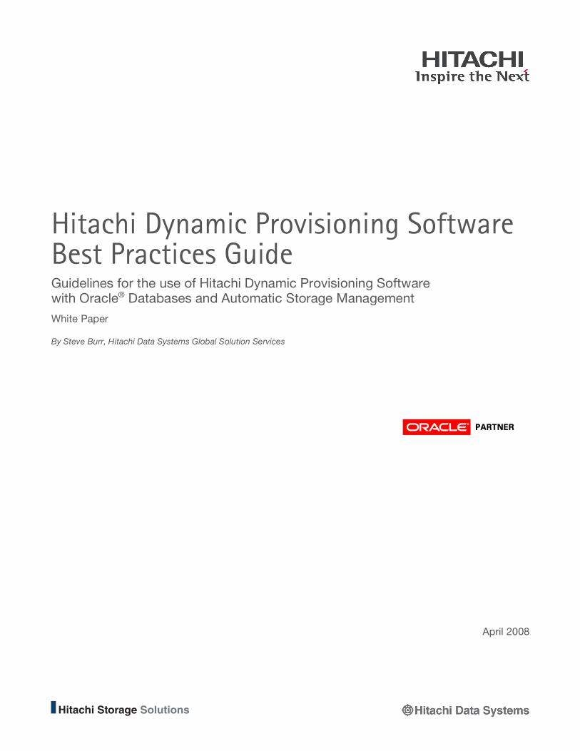
Table 4. Application Capacity and Performance Requirements

Application Capacity Required Application Performance/ Capacity Pattern Small Capacity Large Capacity

Low IOPS

1. Minimum pool size always applies, so this workload must be accommodated by combining it with other applications.

2. This is a good candidate for Hitachi Dynamic Provisioning. It may have spare performance for supporting a high-IOPS application.

Application Performance Needed

High IOPS

3. This is the problematic area as the number of disks needed for performance will exceed the number of disks required for capacity. This workload must be combined with type 1 or type 2 in a common pool.

4. This is a potential candidate for Hitachi Dynamic Provisioning, possibly with a separate pool (or pools).

It is not in the scope of this document to give detailed operations or guidelines for pool design. However, there are a number of standard recommendations:

1. You should not have different drive types for Pool-VOLs registered in a pool.

2. It is a best practice to have the same RAID level for all Pool-VOLs registered to the same pool.

3. For performance reasons, it is best to dedicate array groups to a pool. Four or more array groups are recommended for performance sensitive applications. Distribute array groups evenly over multiple back-end directors if possible.

4. Multiple Pool-DEVs are recommended from each array group. Four are recommended unless you have a large quantity of array groups.

5. Consider pool expansion; do not use the maximum number of Pool-DEVs early.

6. External devices may be used in a pool but should not be in a pool along with internal devices.

7. External Pool-VOLs with different cache modes cannot be intermixed in the same pool.

8. The Pool-DEVs used to construct a pool must be between 8GB and 4TB in size.

9. You cannot remove Pool-DEVs from a pool.

10. Pools should always be initialized (optimized) after creation.

11. Use separate pools for ShadowImage P-VOLs and S-VOLs.

12. Use one DP-VOL in each V-VOL group. This will permit you to resize the DP-VOL, when that feature becomes available.

Additional guidelines are available from your Hitachi Data Systems representative. Also see the “Hitachi Universal Storage Platform™ V and Universal Storage Platform VM Dynamic Provisioning User’s Guide.”

For multiple, large or performance-intensive databases, the performance requirements may justify or require the database to have a separate pool or pools. This is not dissimilar to static provisioning where you might dedicate array groups to an application. Separate pools for each database and separate pool or pools for logs will have benefits but may not always be justifiable unless the capacity is large.

20

Leveraging Performance Leveling Notes

A heavy online transaction processing (OLTP) application might need a peak IOPS requirement that can be met by four array groups in a RAID-10 2+2 configuration. However, the application only requires storage of one array group.

We also have a requirement for a file archive with minimal I/O load but a significant amount of storage, say four array groups.

A possible pool design would be a single Hitachi Dynamic Provisioning pool with five RAID-10 array groups.

Recommendations for Adding Disks to a Pool

The high performance of Hitachi Dynamic Provisioning software is enabled by the fact that a large number of disks are used in the pool. However, if additional disks are added to a pool, data allocated after that time may experience different performance characteristics. The amount of pool left when you add storage will have a significant impact.

Two extreme examples will illustrate this:

Consider a pool constructed from four array groups. All data allocated will have the same performance, four “units.”

1. If all of the pool is used up and then two array groups are added, data allocated after this would have a performance of two units. (This is actually the same as creating a new pool with only two array groups.)

2. If none of the storage is used and two array groups are added, data allocated after this would have a performance of six units. (This is actually the same as creating a new pool with six array groups.)

Obviously, no real environment would have either of these extremes. The recommendations for adding disks to a pool are:

• Do not wait until the last minute to add to the pool unless you plan to add at least the same number of array groups or you are happy that newly allocated data performs more slowly.

• Always add relatively large amounts of storage to the pool.

Oracle Testing Detail This section shows some of the detail of the Oracle testing. The majority of tests were done with Oracle 11g1 RAC on Oracle Enterprise Linux 5. This was chosen as it is the newest database and operating system platform, and it is known to be highly compatible with previous releases. Additional tests were also performed on Oracle 10g2 non-RAC on Solaris, and this confirms that the platforms perform similarly.

A powerful method for understanding how dynamic provisioning is working with an application is a simple graph showing pool space used, compared against space used whilst a number of tests are done on the database.

Multiple quantities correspond to “space used.” This might include sizes of tables, tablespaces, datafiles or diskgroups. As explained previously, these are all contained within one another, the diskgroup being the outermost container. Diskgroup size is therefore the nearest match to pool space used, so it is used in most graphs.

21

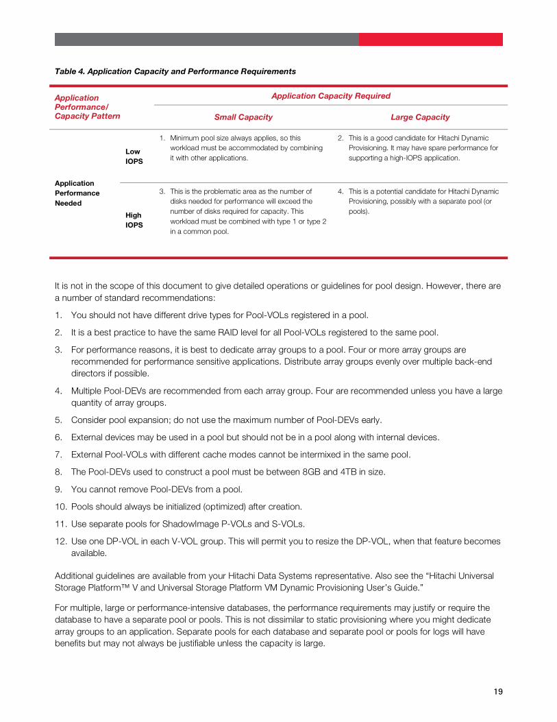
By comparing the two lines we can observe the characteristics of the application. Our hope is for the two lines to stay relatively close together. Although the lines could never be exactly parallel, whether they track one another over the long term is interesting information. Closely tracked lines are the best behavior and what we are looking for. Use of space is rarely uniform; there are steps in the graph. There will be steps in the pool usage graph too but it is very unlikely that they would occur at exactly the same time. Steps in the pool graph will of course be multiples of 42MB.

ASM performs very well; the problem behaviors we needed to rule out were:

1. Pool space initially allocated is a large proportion of the DP-VOL size. The ideal would only have a few percent of overhead. If large amounts are seen, it normally means that the file system is grabbing a lot of pool space for metadata. We would expect the lines to get closer to one another as the file system grows. However, in some cases this is not until the file system is completely full. ASM does not show this behavior. (Sun Solaris UFS and HP-UX HFS exhibit this behavior).

2. Pool space used constantly grows faster than the file system. This most likely indicates that the file system is leaving unused gaps in the disk map. A small diversion is probably acceptable but a large difference may indicate additional strategies need to be followed. ASM does not show this behavior; however, Linux EXT3 and OCFS2 do exhibit this behavior.

3. Pool space used grows faster than the file system but only occurs after file deletions. This indicates that file system disk blocks are not being reused. ASM does not have this behavior. Windows NTFS does have this behavior, so to minimize waste we sometimes need to modify the way the system is configured.

A diskgroup being reduced in size is rarely seen in the ASM graphs below. This is because Oracle rarely reduces the size of objects; space is merely marked as free for reuse. If a datafile is deleted from an ASM diskgroup, then the corresponding line will dip. However, the pool space line will never dip; this is impossible.

Figures 2 through 6 show the amount of space used within an ASM diskgroup (DG) and the equivalent pool space consumed (Pool) during various tests.

Figure 2. Pool versus DG

0

900

MB

DG Pool Table

800

700

600

500

400

300

200

100

Little significant difference is seen between the lines comparing pool space (Pool) and diskgroup data stored (DG).

22

Figure 2 shows growth of the simple table by inserting and deleting rows randomly into a table. Diskgroup size (DG) is shown and should be compared against the pool space allocated (Pool). We are pleased to observe little significant difference between these lines. Note, that the diskgroup does not decrease, even though rows are deleted. The lower line (Table) shows Oracle’s estimate of the data items stored in the table. Towards the end of this run the table was deleted and re-created with compression on. This shows that compression has no adverse effects on Hitachi Dynamic Provisioning.

Figure 3. Multiple Tables per Tablespace

0

MB

DG Pool

500

450

400

350

300

250

200

150

100

50

Testing multiple tables in the tablespace showed good results, with no additional issues due to multiple objects.

Figure 3 shows a test similar to the one in Figure 2 but with multiple tables in the tablespace. By testing these tables in parallel we ensure that multiple objects do not cause additional issues. The results were similarly good.

Figure 4. Multiple Tablespaces per Diskgroup and Drop/Recreate Tablespaces

0

MB

DG Pool

500

450

400

350

300

250

200

150

100

50

Dropping and creating tables and tablespaces showed similarly good results.

23

Figure 4 shows a similar test to those above but with multiple tablespaces in the diskgroup. We also dropped and created tables and tablespaces. The results were similarly good.

Figure 5. Archive Redo Log Files

GB

Pool Archive Redo

3.0

2.5

2.0

1.5

1.0

0.5

0.0

The BACKUP diskgroup is used for non-tablespace data.

The test results in Figure 5 show a different diskgroup, BACKUP, which is used for non-tablespace data, such as archive redo log files and flashsnap data. These files are dynamic in character, which would show up poor reclaim. During database operation and management archive redo log files are continuously created and deleted. The space used for archive redo files increases as transactions are performed on the database; they are deleted by RMAN when backups occur. Again, ASM is shown completely efficient in space usage.

Figure 6. Space Usage against Row Count

00

MB

DG Pool DG' Pool'

450

400

350

300

250

200

150

100

50

100000 200000 300000 400000 500000 600000 700000

Trend lines have been added to the row count lines to show linearity of growth.

24

Figure 6 uses a different X-axis, row count; previous graphs used time. Also added to the graph are trend lines. These make the relatively small pool overhead and the linearity of the growth much clearer.

Hitachi Dynamic Provisioning and Hitachi Replication Products Hitachi Dynamic Provisioning currently supports replication with Hitachi ShadowImage Heterogeneous Replication software but will soon support most other replication products such as Hitachi TrueCopy Synchronous/Asynchronous, Universal Replicator, Copy-on-Write Snapshot and Volume Migration software (Contact Hitachi Data Systems for the latest Hitachi replication products supported by Hitachi Dynamic Provisioning). You would nearly always use Hitachi Dynamic Provisioning software to provision volumes for both the primary and secondary volumes. ShadowImage Heterogeneous Replication software is aware of which areas of the volumes are and are not allocated. The configured size of both volumes must be the same. If you use ShadowImage to copy a volume, the copy will be equally space efficient. Hitachi HiCommand Protection Manager, when used with ShadowImage Replication software will also operate efficiently. To minimize contention and maintain best efficiency, ShadowImage secondary volumes should use a different pool from the primary. Restore actions should not consume additional space as the volume has been derived from the primary. The only exception might be if a secondary volume was mounted and then changed significantly, increasing pool space of the secondary volume. If restored, the primary would also increase in size.

Example: We are using Hitachi Dynamic Provisioning on an Oracle database. The volumes are sized at 1TB for future expansion, but they currently have 300GB of space allocated. By using Hitachi SplitSecond Solutions to back up the database we can take a backup in a matter of seconds without any disruption to users. Further, the ShadowImage DP-VOLs used to back up the database will be on volumes configured to 1TB, but would also only have 300GB of space allocated.

Compared to static provisioning in the above example, we are saving 700GB for the database plus 700GB for each backup.

When using the Hitachi replication products, it is important not to run out of shared memory capacity. All the replication products use an amount of shared memory, which is dependant on the volume size and the number of pairs. This size is the Virtual Volume (DP-VOL) configured size, not the pool quantity used. Therefore, if you aggressively overprovision volumes and then use them with replication products, you will consume shared memory more rapidly and may run out. All replication products that have “pairs” use shared memory. This includes: ShadowImage Heterogeneous Replication, TrueCopy Synchronous/Asynchronous, Universal Replicator, Copy-on-Write Snapshot and Volume Migration software.

Management Tasks This section considers management tasks performed on overprovisioned dynamic provisioned volumes.

Whilst you remain within an ASM environment there seems to be little danger of the pool space outstripping the space actually used. However, if there are no limits in place then there is a slight danger of making mistakes. For example, if we drop a table with the intention of re-creating it, then, in most cases, this would re-use the space just freed. This will always occur if Oracle Managed Files are used. If Oracle Managed Files are not used the following syntax can be used to delete everything: DROP TABLESPACE X INCLUDING CONTENTS AND DATAFILES. It is recommended that you query one of the system views or use ASMCMD to check that space

25

has actually been deleted before performing major activities such as importing a large data or a major table insert. For example, SELECT FREE_MB, TOTAL_MB, NAME FROM V$ASM_DISKGROUP.

If the DP-VOLs are to be fully allocated or are capped by some method (partition or diskgroup size definition), these recommendations are not needed.

If by mistake too much data is allocated to a volume and you need to reclaim all the space, then the volume needs to be completely first deleted from the server and second deleted from the storage to free the pool usage. There are many possibilities, but one process that leaves the database online all the time might be:

1. Create a new DP-VOL. See the Dynamic Provisioning User’s Guide for details on this.

2. Associate this with a pool that has sufficient capacity to hold the data you need to preserve. Ideally, this will be the same as the original pool, to remove the chance of any performance differences.

3. Map this DP-VOL to the server and follow the normal process for initialization of an ASM disk.

4. If RAC is used ensure that all nodes are aware of the changes.

5. Add the new disk to the problem diskgroup (ALTER DISKGROUP X ADD DISK N;). This will start a rebalance operation.

6. Wait until the rebalance has finished. Then drop the problem disk (ALTER DISKGROUP X DROP DISK P;). A second rebalance will occur.

7. Wait until the rebalance has finished. Then you can remove the disk from ASM completely.

8. Remove from path management.

9. Remove from the operating system.

10. Use Storage Navigator to remove all LUN paths to the problem DP-VOL.

11. Perform LDEV formatting on the DP-VOL. For specific instructions on LDEV formatting see the Virtual LVI/LUN and Volume Shredder User’s Guide.

12. Release the association between the DP-VOL and the pool.

13. Delete the DP-VOL.

Monitoring You may wish to monitor the use of Hitachi Dynamic Provisioning pools quite carefully. There are several techniques available:

1. The Dynamic Provisioning software will generate alerts if the pool exceeds its configured thresholds.

2. The above alerts can be configured to be passed through SNMP TRAPs to your management system.

3. Hitachi HiCommand Tuning Manager software has additional features for reporting the trends of pool and LDEV usage. See “HiCommand® Tuning Manager Hardware Reports Reference” for more details.

4. In addition, you can configure HiCommand Tuning Manager to generate alerts when usage exceeds configured values or if usage trends look dangerous.

5. RAID Manager can be used to report on pool and individual DP-VOL usage. This can be used to develop custom monitoring solutions and is a valuable tactical tool for “what is the current status”.

6. You may wish to combine the above monitoring with scripts to adjust dynamic partitions.

26

RAID Manager Monitoring RAID Manager can give you an instantaneous view of pool usage at the DP-VOL and pool level.

raidvchkdsp —g HDP —fx —v aou

Group PairVol Port# TID LU Seq# LDEV# Used (MB) LU_CAP (MB) U(%) T(%) PID

HDP MDF CL6-B-1 18 35 10044 b906 2814 93750 1 70 9

HDP LDF CL6-B-1 18 36 10044 b907 4032 93750 1 70 9

HDP AUX CL6-B-1 18 37 10044 b908 8442 93750 1 70 9

The above report shows the status of a group configured in RAID Manager. Suitable Group and PairVol names have been chosen to help identify the use. If groups are not configured, then the similar raidvchkscan command can be used. The first data line shows: Group HDP contains a Volume MDF. This is mapped as Host Storage Domain CL6-B-1, target ID 18 and LUN 35. The storage serial number is 10044 and the LDEV number is hex B906. The application (SQL Server, MDF file) has used 2814MB of the allocated capacity 93750MB. The pool threshold is 70 percent. This volume is associated with pool 9, and 1 percent of this pool is currently used. Note: the threshold and usage are for the total pool, not the LDEV. To get LDEV usage ratio, you need to divide 2814 by 93750.

raidvchkscan -v pida

PID POLS U(%) AV_CAP(MB) TP_CAP(MB) W(%) H(%) Num LDEV# LCNT TL_CAP (MB)

009 POLN 1 819714 820302 80 70 16 40 104 3334687

010 POLN 0 3286038 3286038 80 70 64 28672 154 11426142

The above report shows the status of the pools on the attached storage. The first data line shows: pool 9 is in a normal state (POLN), 1 percent of the pool has been used, 819,714MB is available from a starting size of 820,302MB. The warning threshold is 80 percent and the high water mark is 70 percent. There are 16 LDEVs in this pool and the first pool volume is LDEV 40. The pool has 104 DP-VOLs using it; they are configured to be able to expand up to 3334687MB. However, 3334687MB is greater than 820302MB, so we cannot grow the volumes to this size without increasing the pool size first. We would call this an overprovisioned pool.

For more information on RAID Manager commands see: “Hitachi Command Control Interface (CCI) User and Reference Guide.”

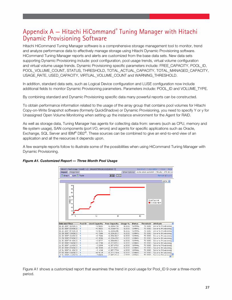
27

Appendix A — Hitachi HiCommand® Tuning Manager with Hitachi Dynamic Provisioning Software Hitachi HiCommand Tuning Manager software is a comprehensive storage management tool to monitor, trend and analyze performance data to effectively manage storage using Hitachi Dynamic Provisioning software. HiCommand Tuning Manager reports and alerts are customized from the base data sets. New data sets supporting Dynamic Provisioning include: pool configuration, pool usage trends, virtual volume configuration and virtual volume usage trends. Dynamic Provisioning specific parameters include: FREE_CAPACITY, POOL_ID, POOL_VOLUME_COUNT, STATUS, THRESHOLD, TOTAL_ACTUAL_CAPACITY, TOTAL_MANAGED_CAPACITY, USAGE_RATE, USED_CAPACITY, VIRTUAL_VOLUME_COUNT and WARNING_THRESHOLD.

In addition, standard data sets, such as Logical Device configuration and LUSE configuration now include additional fields to monitor Dynamic Provisioning parameters. Parameters include: POOL_ID and VOLUME_TYPE.

By combining standard and Dynamic Provisioning specific data many powerful reports can be constructed.

To obtain performance information related to the usage of the array group that contains pool volumes for Hitachi Copy-on-Write Snapshot software (formerly QuickShadow) or Dynamic Provisioning, you need to specify Y or y for Unassigned Open Volume Monitoring when setting up the instance environment for the Agent for RAID.

As well as storage data, Tuning Manager has agents for collecting data from: servers (such as CPU, memory and file system usage), SAN components (port I/O, errors) and agents for specific applications such as Oracle, Exchange, SQL Server and IBM® DB2®. These sources can be combined to give an end-to-end view of an application and all the resources it depends upon.

A few example reports follow to illustrate some of the possibilities when using HiCommand Tuning Manager with Dynamic Provisioning.

Figure A1. Customized Report — Three Month Pool Usage

Figure A1 shows a customized report that examines the trend in pool usage for Pool_ID 9 over a three-month period.

28

Customized alerts can be created to monitor pool usage in a number of ways. If thresholds are exceeded then one of the following options can be configured:

• Sending of an e-mail

• Raising of a system alert

• Creating an SNMP TRAP

• Running a program: possibly one to use Hitachi HiCommand Device Manager scripting to configure additional storage for the pool.

Figure A2. Virtual Volume Pool Usage Report

Figure A2 shows the trend of pool usage for a selected range of Virtual Logical devices that use a specified pool.

LDEV 00:01:04 is growing rapidly and is already 60 percent of its configured capacity.

29

Figure A3. Standard Report

Of course standard Tuning Manager reports are also of value when analyzing Dynamic Provisioning data.

Drive group reports such as the screen shown in Figure A3 will be relevant for monitoring the performance of both static provisioned volumes and array groups allocated to Hitachi Dynamic Provisioning pools.

Data on the performance or use of V-VOL groups are not included in any of the standard reports; this would have little benefit as the V-VOL group has no physical significance.

In a similar way, standard or customized LDEV reports can be used to monitor:

• Static provisioned LDEVs

• Dynamic provisioned LDEVs

• LDEVs used to construct dynamic provisioning pools

30

Appendix B — Hitachi Dynamic Provisioning Software Terms The following Hitachi Dynamic Provisioning terminology and their respective definitions have been used throughout this paper:

• RAID Group — a grouping of multiple disk drives combined to form a single pool of data with a specified RAID level.

• LDEV (Logical Device) — a volume created from the space within a particular array group. An LDEV is partitioned from that array group’s raw space.

• HDP Pool (pool) — a pool of physical storage capacity that is allocated to dynamic provisioned virtual volumes (DP-VOLs). The actual data is stored here in 42MB pages and it is also referred to within this document simply as “pool.”

• Pool Volume (Pool-VOL) — a regular LDEV used to construct a pool. For performance reasons a pool will normally have multiple pool volumes from multiple array groups.

• V-VOL (Virtual Volume) — a volume where space is not allocated statically at creation. Only the maximum size is specified, up to 2TB. Space will be allocated from a pool as it is required. Hitachi Dynamic Provisioning and Hitachi Copy-on-Write Snapshot software products currently use V-VOLs.

• DP-VOL (Dynamic Provisioned Virtual Volume) — a Hitachi Dynamic Provisioning volume created from an HDP pool. It is one of the virtual volume types supported by the Universal Storage Platform V and Universal Storage Platform VM. A DP-VOL is a member of a V-VOL group.

• LUN (Logical Unit Number) — the host-visible identifier assigned by the user to an LDEV when mapped to a Storage Port or Host Storage Domain.

• V-VOL Group — a container for virtual volumes. One or more V-VOLs are configured within this space, each with a specified maximum size. The total of these sizes must be less than the size of the V-VOL Group. The maximum size currently supported for a V-VOL Group is 3TB. A V-VOL Group can be thought of as a virtual array group (in reports a normal array group might show as 2-4, a dynamic provisioned V-VOL group as X5-1 and a Copy-on-Write Snapshot V-VOL group as V2-1).

• Static Provisioning — making early and largely unchangeable decisions about storage usage. Physical location, reliability, performance and cost are fixed at the time the data is made available to the server (sometimes earlier: at initial purchase). These design decisions generally freeze that data’s performance and capacity. Contrast with:

• Dynamic Provisioning — using Hitachi Dynamic Provisioning software to delay or modify decisions about storage usage until actually needed by the application. This allows capacity, performance and cost to be optimized as the application evolves. Dynamic Provisioning is the ultimate concept in virtualization of storage. Hitachi Dynamic Provisioning software uses thin-provisioning techniques but is able to deliver more. Hitachi Dynamic Provisioning software also supports additional virtualization through: tiered storage, online data migration and multiple storage pools; this gives greatly increased flexibility and control over both capacity and performance.

• Thin Provisioning (occasionally sparse volumes) — a technique of dynamically allocating storage blocks only when the application writes to a specific area of (virtual) storage. Storage thin provisioning is a logical evolution of techniques developed for virtualizing server memory developed by IBM in the 1960s. Thin provisioning is one aspect of Hitachi Dynamic Provisioning software. It is supported by a number of storage vendors.

• Overprovisioned (overallocated, oversubscribed) — where more space is allocated to a storage volume, and therefore to a server, than you currently require.

31

• Wide Striping — leveraging the pooling effect you get when multiple applications use a common pool. Application data is striped across all physical disk spindles in the pool, giving very high peak performance. All applications in the pool are able to share this.

Hitachi Data Systems Corporation

Corporate Headquarters 750 Central Expressway, Santa Clara, California 95050-2627 USA Contact Information: + 1 408 970 1000 www.hds.com / info@hds.com

Asia Pacific and Americas 750 Central Expressway, Santa Clara, California 95050-2627 USA

Contact Information: + 1 408 970 1000 www.hds.com / info@hds.com

Europe Headquarters Sefton Park, Stoke Poges, Buckinghamshire SL2 4HD United Kingdom

Contact Information: + 44 (0) 1753 618000 www.hds.com / info.uk@hds.com Hitachi is a registered trademark of Hitachi, Ltd., and/or its affiliates in the United States and other countries. Hitachi Data Systems is a registered trademark and service mark of Hitachi, Ltd., in the United States and other countries. HiCommand is a registered trademark of Hitachi, Ltd.

TrueCopy and ShadowImage are registered trademarks and Universal Storage Platform and SplitSecond are trademarks of Hitachi Data Systems Corporation.

Oracle is a registered trademark of Oracle Corporation and/or its affiliates.

IBM and DB2 are registered trademarks of International Business Machines Corporation.

Microsoft is a registered trademark of Microsoft Corporation.

All other trademarks, service marks and company names are properties of their respective owners.

Notice: This document is for informational purposes only, and does not set forth any warranty, express or implied, concerning any equipment or service offered or to be offered by Hitachi Data Systems. This document describes some capabilities that are conditioned on a maintenance contract with Hitachi Data Systems being in effect, and that may be configuration-dependent, and features that may not be currently available. Contact your local Hitachi Data Systems sales office for information on feature and product availability.

Hitachi Data Systems sells and licenses its products subject to certain terms and conditions, including limited warranties. To see a copy of these terms and conditions prior to purchase or license, please go to http://www.hds.com/corporate/legal/index.html or call your local sales representative to obtain a printed copy. If you purchase or license the product, you are deemed to have accepted these terms and conditions.

© Hitachi Data Systems Corporation 2008. All Rights Reserved WHP-277-01 KLD April 2008