Embed Size (px)
Citation preview
Hit-and-Run is Fast and Fun 1
Laszlo Lovasz2 Santosh Vempala3
January 2003
Technical ReportMSR-TR-2003-05
The hit-and-run algorithm is one of the fastest known methods to gener-
ate a random point in a high dimensional convex set. In this paper we
study a natural extension of the hit-and-run algorithm to sampling from a
logconcave distribution in n dimensions. After appropriate preprocessing,
hit-and-run produces a point from approximately the right distribution in
amortized time O∗(n3).
Microsoft ResearchMicrosoft CorporationOne Microsoft Way
Redmond, WA 98052http://www.research.microsoft.com
1Part of this work was done while the second author was visiting Microsoft Researchin Redmond, WA, and when the first author was visiting the Newton Institute inCambridge, UK.
2Microsoft Research, One Microsoft Way, Redmond, WA 980523Department of Mathematics, Massachusetts Institute of Technology, Cambridge,
MA 02139. Supported by NSF Career award CCR-9875024.
1 Introduction
In recent years, the problem of sampling a convex body has received muchattention, and many efficient solutions have been proposed [4, 7, 12, 10, 9], allbased on random walks. Of these, the hit-and-run random walk, first proposedby Smith [19], has the same worst-case time complexity as the more thoroughlyanalyzed ball walk, but seems to be fastest in practice.
The random walk approach for sampling can be extended to the class oflogconcave distributions. For our purposes, it suffices to define these as proba-bility distributions on the Borel sets of Rn which have a density function f andthe logarithm of f is concave. Such density functions play an important rolein stochastic optimization [17] and other applications [8]. We assume that thefunction is given by an oracle, i.e., by a subroutine that returns the value of thefunction at any point x. We measure the complexity of the algorithm by thenumber of oracle calls.
For the lattice walk and the ball walk, the extension to logconcave functionswas introduced and analyzed in [1, 6] under additional smoothness assumptionsabout the density function. In [15], it was shown that the ball walk can beused without such assumptions, with running time bounds that are essentiallythe same as for sampling from convex bodies. In this paper we analyze thebehavior of the hit-and-run walk for logconcave distributions. Our main resultis that after appropriate preprocessing (bringing the distribution to isotropicposition), we can generate a sample using O∗(n4) steps (oracle calls) and inO∗(n3) steps from a warm start. (This means that we start the walk from arandom point whose density function is at most a constant factor larger thanthe target density f ; cf. [15].) As in [15], we make no assumptions on thesmoothness of the density function. The analysis uses the smoothing techniqueintroduced in [15], and in main lines of follows the analysis of the hit-and-runwalk in [13], with substantial additional difficulties.
2 Results
2.1 Preliminaries.
A function f : Rn → R+ is logconcave if it satisfies
f(αx + (1− α)y) ≥ f(x)αf(y)1−α
for every x, y ∈ Rn and 0 ≤ α ≤ 1. This is equivalent to saying that the supportK of f is convex and log f is concave on K.
An integrable function f : Rn → R+ is a density function, if∫Rn f(x) dx = 1.
Every non-negative integrable function f gives rise to a probability measure onthe measurable subsets of Rn defined by
πf (S) =∫
S
f(x) dx
/∫
Rn
f(x) dx .
1
The centroid of a density function f : Rn → R+ is the point
zf =∫
Rn
f(x)x dx;
the covariance matrix of the function f is the matrix
Vf =∫
Rn
f(x)xxT dx
(we assume that these integrals exist).For any logconcave function f : R → Rn, we denote by Mf its maximum
value. We denote byLf (t) = {x ∈ Rn : f(x) ≥ t}
its level sets, and by
ft(x) ={
f(x), if f(x) ≥ t,0, if f(x) < t,
its restriction to the level set. It is easy to see that ft is logconcave. In Mf andLf we omit the subscript if f is understood.
A density function f : Rn → R+ is isotropic, if its centroid is 0, and itscovariance matrix is the identity matrix. This latter condition can be expressedin terms of the coordinate functions as
∫
Rn
xixjf(x) dx = δij
for all 1 ≤ i, j ≤ n. This condition is equivalent to saying that for every vectorv ∈ Rn, ∫
Rn
(v · x)2f(x) dx = |v|2.
In terms of the associated random variable X, this means that
E(X) = 0 and E(XXT ) = I.
We say that f is near-isotropic up to a factor of C, if (1/C) ≤ ∫(uT x)2 dπf (x) ≤
C for every unit vector u. As in [15], the notions of “isotropic” and “non-isotropic” extend to non-negative integrable functions f , in which case we meanthat the density function f/
∫Rn f is isotropic or near-isotropic.
Given any density function f with finite second moment∫Rn ‖x‖2f(x) dx,
there is an affine transformation of the space bringing it to isotropic position,and this transformation is unique up to an orthogonal transformation of thespace.
For two points u, v ∈ Rn, we denote by d(u, v) their euclidean distance. Fortwo probability distributions σ, τ on the same underlying σ-algebra, let
dtv(σ, τ) = supA
(σ(A)− τ(A))
be their total variation distance.
2
2.2 The random walk.
Let f be a logconcave distribution in Rn. For any line ` in Rn, let µ`,f be themeasure induced by f on `, i.e.
µ`,f (S) =∫
p+tu∈S
f(p + tu)dt,
where p is any point on ` and u is a unit vector parallel to `. We abbreviateµ`,f by µ` if f is understood, and also µ`(`) by µ`. The probability measureπ`(S) = µ`(S)/µ` is the restriction of f to `.
We study the following generalization of the hit-and-run random walk.
• Pick a uniformly distributed random line ` through the current point.
• Move to a random point y along the line ` chosen from the distributionπ`.
Let us remark that the first step is easy to implement. For example, we cangenerate n independent random numbers U1, . . . , Un from the standard normaldistribution, and use the vector (U1, . . . , Un) to determine the direction of theline.
In connection with the second step, we have to discuss how the function isgiven: we assume that it is given by an oracle. This means that for any x ∈ Rn,the oracle returns the value f(x). (We ignore here the issue that if the valueof the function is irrational, the oracle only returns an approximation of f .) Itwould be enough to have an oracle which returns the value C · f(x) for someunknown constant C > 0 (this situation occurs in many sampling problems e.g.in statistical mechanics and simulated annealing).
For technical reasons, we also need a “guarantee” from the oracle that thecentroid zf of f satisfies ‖zf‖ ≤ Z and that all the eigenvalues of the covariancematrix are between r and R, where Z, r and R are given positive numbers.
One way to carry out the second step is to use a binary search to find thepoint p on ` where the function is maximal, and the points a and b on both sidesof p on ` where the value of the function is εf(p). We allow a relative error ofε, so the number of oracle calls is only O(log(1/ε)).
Then select a uniformly distributed random point y on the segment [a, b],and independently a uniformly distributed random real number in the interval[0, 1]. Accept y if f(y) > rf(p); else, reject y and repeat.
The distribution of the point generated this way is closer to the desired dis-tribution than ε, and the expected number of oracle calls needed is O(log(1/ε)).
Our main theorem concerns functions that are near-isotropic (up to somefixed constant factor c).
Theorem 2.1 Let f be a logconcave density function in Rn that is near-isotropic up to a factor of c. Let σ be a starting distribution and let σm be
3
the distribution of the current point after m steps of the hit-and-run walk. As-sume that there is a D > 0 such that σ(S) ≤ Dπf (S) for every set S. Thenfor
m > 1010c2D2 n3
ε2log
1ε,
the total variation distance of σm and πf is less than ε.
2.3 Distance and Isoperimetry.
To analyze the hit-and-run walk, we need a notion of distance according toa density function. Let f be a logconcave density function. For two pointsu, v ∈ Rn, let `(u, v) denote the line through them. Let [u, v] denote the segmentconnecting u and v, and let `+(u, v) denote the semiline in ` starting at u andnot containing v. Furthermore, let
f+(u, v) = µ`,f (`+(u, v)),f−(u, v) = µ`,f (`+(v, u)),
f(u, v) = µ`,f ([u, v]).
We introduce the following “distance”:
df (u, v) =f(u, v)f(`(u, v))f−(u, v)f+(u, v)
.
The function df (u, v) does not satisfy the triangle inequality in general, butwe could take ln(1 − df (u, v)) instead, and this quantity would be a metric;however, it will be more convenient to work with df .
Suppose f is the uniform distribution over a convex set K. Let u, v be twopoints in K and p, q be the endpoints of `(u, v) ∩K, so that the points appearin the order p, u, v, q along `(u, v). Then,
df (u, v) = dK(u, v) =|u− v||p− q||p− u||v − q| .
2.4 An isoperimetric inequality
The next theorem is an extension of Theorem 6 from [13] to logconcave functions.
Theorem 2.2 Let f be a logconcave density function on Rn with support K.For any partition of K into three measurable sets S1, S2, S3,
πf (S3) ≥ dK(S1, S2)πf (S1)πf (S2).
3 Preliminaries
3.1 Spheres and balls
Lemma 3.1 Let H be a halfspace in Rn and B, a ball whose center is at adistance t > 0 from H. Then
4
(a) if t ≤ 1/√
n, then
vol(H ∩B) >
(12− t
√n
2
)vol(B);
(b) if t > 1/√
n then
110t√
n(1− t2)(n+1)/2vol(B) < vol(H ∩B) <
1t√
n(1− t2)(n+1)/2vol(B).
Let C be a cap on the unit sphere S in Rn, with radius r and voln−1(C) =cvoln−1(S), c < 1/2. We can write its radius as r = π/2 − t(c). The functiont(c) is difficult to express exactly, but for our purposes, the following knownbounds will be enough:
Lemma 3.2 If 0 < c < 2−n, then
12c1/n < t(c) < 2c1/n;
if 2−n < c < 1/4, then
12
√ln(1/c)
n< t(c) < 2
√ln(1/c)
n;
if 1/4 < c < 1/2, then
12
(12− c
)1√n
< t(c) < 2(
12− c
)1√n
.
Using this function t(c), we can formulate a fact that can be called ”strongexpansion” on the sphere:
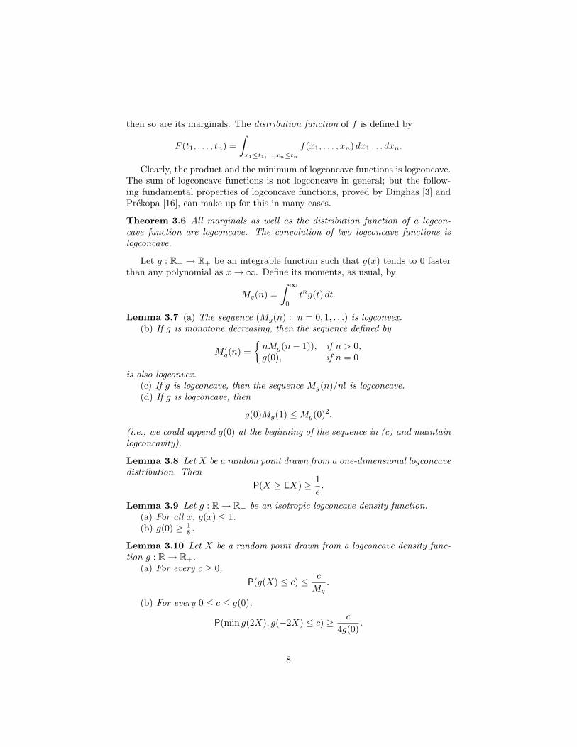
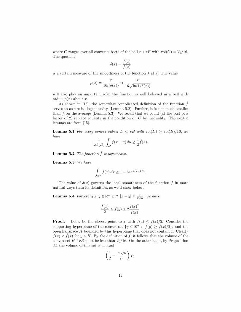
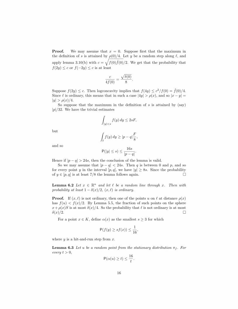
Lemma 3.3 Let T1 and T2 be two sets on the unit sphere S in Rn, so thatvoln−1(Ti) = civoln−1(S). Then the angular distance between T1 and T2 is atmost t(c1) + t(c2).
Proof. Let d denote the angular distance between T1 and T2. The measureof Ti corresponds to the measure of a spherical cap with radius π/2− t(c1). Byspherical isoperimetry, the measure of the d-neighborhood of T1 is at least aslarge as the measure of the d-neighborhood of the corresponding cap, which isa cap with radius π/2 − t(c1) + d. The complementary cap has radius π/2 +t(c1)− d and volume at least c2, and so it has radius at least π/2− t(c2). Thusπ/2 + t(c1)− d ≥ π/2− t(c2), which proves the lemma. ¤
Lemma 3.4 Let K be a convex body in Rn containing the unit ball B, and letr > 1. If φ(r) denotes the fraction of the sphere rS that is contained in K, then
t(1− φ(r)) + t(φ(2r)) ≥ 38r
.
5
T1
t(c1)
t(c2)
T2
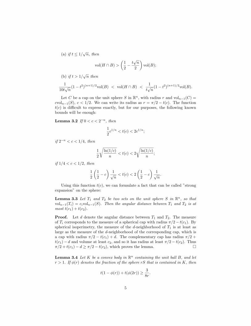
Figure 1: Caps at maximal angular distance.
Proof. Let T1 = (rS) ∩ K and T2 = (1/2)((2rS) \ K). We claim that theangular distance of T1 and T2 is at least 3/(8r). Consider any y1 ∈ T1 andy2 ∈ T2, we want to prove that the angle α between them is at least 3/(8r). Wemay assume that this angle is less than π/4 (else, we have nothing to prove).Let y0 be the nearest point to 0 on the line through 2y2 and y1. Then y0 /∈ Kby convexity, and so s = |y0| > 1. Let αi denote the angle between yi and y0.Then
sinα = sin(α2 − α1) = sin α2 cosα1 − sin α1 cos α2.
Here cos α1 = s/r and cos α1 = s/(2r); expressing the sines and substituting,we get
sin α =s
r
√1− s2
4r2− s
2r
√1− s2
r2.
To estimate this by standard tricks from below:
sin α =
s2
r2
(1− s2
4r2
)− s2
4r2
(1− s2
r2
)
s
r
√1− s2
4r2+
s
2r
√1− s2
r2
>
s2
r2
(1− s2
4r2
)− s2
4r2
(1− s2
r2
)
s
r+
s
2r
=s
2r>
12r
Since α > sinα, this proves the lemma. ¤The way this lemma is used is exemplified by the following:
6
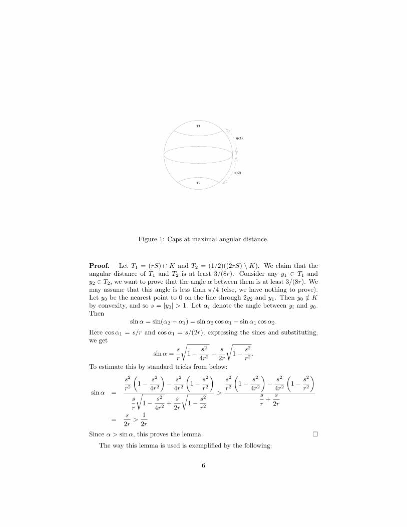
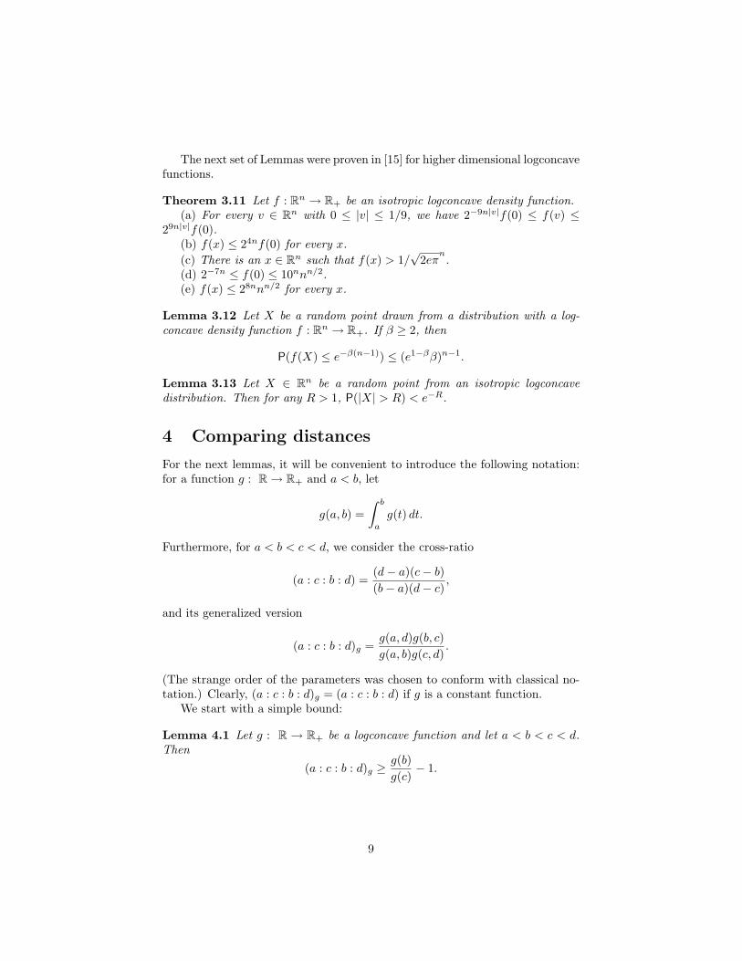
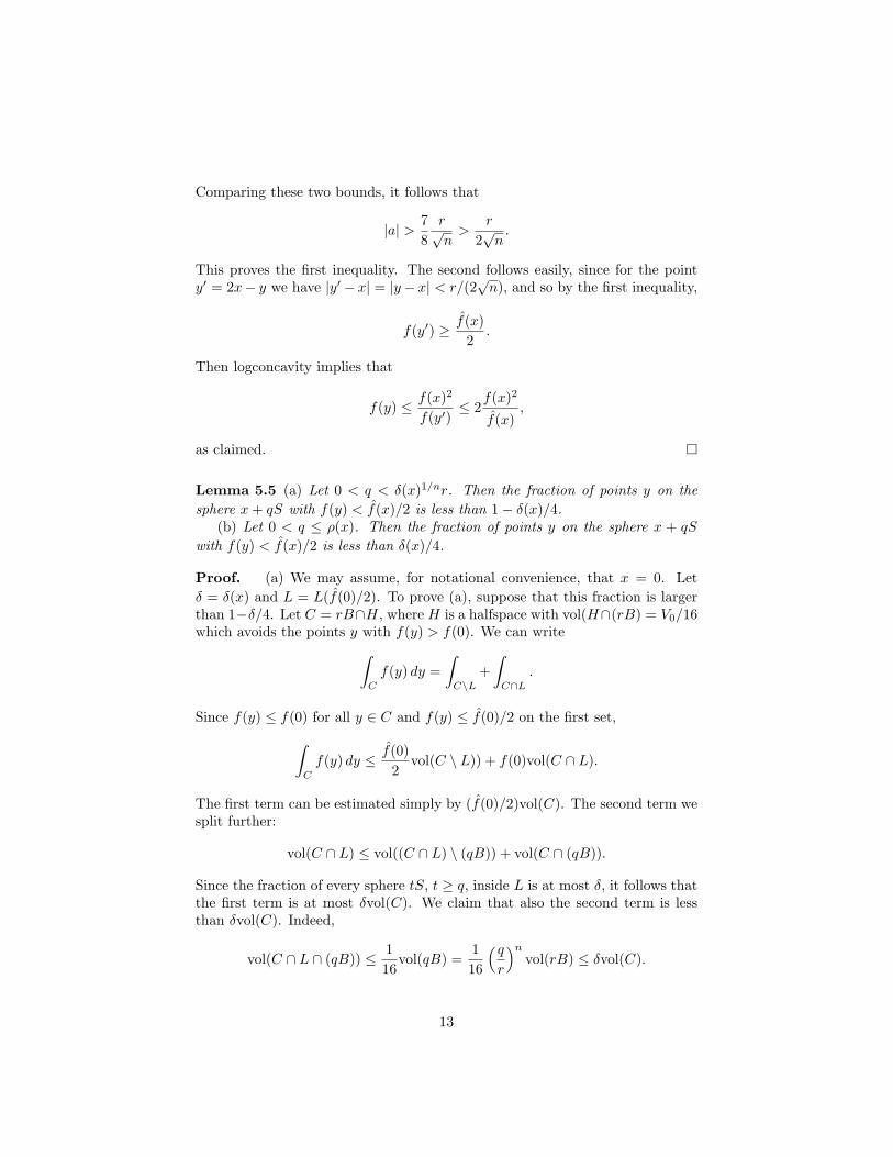
Corollary 3.5 Let K be a convex body in Rn containing the unit ball B, andlet 1 < r <
√n/10. If K misses 1% of the sphere rS, then it misses at least
99% of the sphere 2rS.
K
2rr
Figure 2: An illustration of Corollary 3.5.
3.2 Logconcave functions: a recap
In this section we recall some folklore geometric properties of logconcave func-tions as well as some that were proved in [15].
We need some definitions. The marginals of a function f : Rn → R+ aredefined by
G(x1, . . . , xk) =∫
Rn−k
f(x1, . . . , xn) dxk+1 . . . dxn.
The first marginal
g(t) =∫
x2,...,xn
f(t, x2, . . . , xn) dx2 . . . dxn
will be used most often. It is easy to check that if f is in isotropic position,
7
then so are its marginals. The distribution function of f is defined by
F (t1, . . . , tn) =∫
x1≤t1,...,xn≤tn
f(x1, . . . , xn) dx1 . . . dxn.
Clearly, the product and the minimum of logconcave functions is logconcave.The sum of logconcave functions is not logconcave in general; but the follow-ing fundamental properties of logconcave functions, proved by Dinghas [3] andPrekopa [16], can make up for this in many cases.
Theorem 3.6 All marginals as well as the distribution function of a logcon-cave function are logconcave. The convolution of two logconcave functions islogconcave.
Let g : R+ → R+ be an integrable function such that g(x) tends to 0 fasterthan any polynomial as x →∞. Define its moments, as usual, by
Mg(n) =∫ ∞
0
tng(t) dt.
Lemma 3.7 (a) The sequence (Mg(n) : n = 0, 1, . . .) is logconvex.(b) If g is monotone decreasing, then the sequence defined by
M ′g(n) =
{nMg(n− 1)), if n > 0,g(0), if n = 0
is also logconvex.(c) If g is logconcave, then the sequence Mg(n)/n! is logconcave.(d) If g is logconcave, then
g(0)Mg(1) ≤ Mg(0)2.
(i.e., we could append g(0) at the beginning of the sequence in (c) and maintainlogconcavity).
Lemma 3.8 Let X be a random point drawn from a one-dimensional logconcavedistribution. Then
P(X ≥ EX) ≥ 1e.
Lemma 3.9 Let g : R→ R+ be an isotropic logconcave density function.(a) For all x, g(x) ≤ 1.(b) g(0) ≥ 1
8 .
Lemma 3.10 Let X be a random point drawn from a logconcave density func-tion g : R→ R+.
(a) For every c ≥ 0,P(g(X) ≤ c) ≤ c
Mg.
(b) For every 0 ≤ c ≤ g(0),
P(min g(2X), g(−2X) ≤ c) ≥ c
4g(0).
8
The next set of Lemmas were proven in [15] for higher dimensional logconcavefunctions.
Theorem 3.11 Let f : Rn → R+ be an isotropic logconcave density function.(a) For every v ∈ Rn with 0 ≤ |v| ≤ 1/9, we have 2−9n|v|f(0) ≤ f(v) ≤
29n|v|f(0).(b) f(x) ≤ 24nf(0) for every x.(c) There is an x ∈ Rn such that f(x) > 1/
√2eπ
n.
(d) 2−7n ≤ f(0) ≤ 10nnn/2.(e) f(x) ≤ 28nnn/2 for every x.
Lemma 3.12 Let X be a random point drawn from a distribution with a log-concave density function f : Rn → R+. If β ≥ 2, then
P(f(X) ≤ e−β(n−1)) ≤ (e1−ββ)n−1.
Lemma 3.13 Let X ∈ Rn be a random point from an isotropic logconcavedistribution. Then for any R > 1, P(|X| > R) < e−R.
4 Comparing distances
For the next lemmas, it will be convenient to introduce the following notation:for a function g : R→ R+ and a < b, let
g(a, b) =∫ b
a
g(t) dt.
Furthermore, for a < b < c < d, we consider the cross-ratio
(a : c : b : d) =(d− a)(c− b)(b− a)(d− c)
,
and its generalized version
(a : c : b : d)g =g(a, d)g(b, c)g(a, b)g(c, d)
.
(The strange order of the parameters was chosen to conform with classical no-tation.) Clearly, (a : c : b : d)g = (a : c : b : d) if g is a constant function.
We start with a simple bound:
Lemma 4.1 Let g : R → R+ be a logconcave function and let a < b < c < d.Then
(a : c : b : d)g ≥ g(b)g(c)
− 1.
9
Proof. We may assume that g(b) > g(c) (else, there is nothing to prove).Let h(t) be an exponential function such that h(b) = g(b) and h(c) = g(c). Bylogconcavity, g(x) ≤ h(x) for x ≤ a and g(x) ≥ h(x) for b ≤ x ≤ c. Hence
(a : c : b : d)g =g(a, d)g(b, c)g(a, b)g(c, d)
≥ g(b, c)g(a, b)
≥ h(b, c)h(a, b)
=h(c)− h(b)h(b)− h(a)
≥ h(c)− h(b)h(b)
=g(b)g(c)
− 1.
¤
Lemma 4.2 Let g : R → R+ be a logconcave function and let a < b < c < d.Then
(a : c : b : d)g ≥ (a : c : b : d).
Proof. By Lemma 2.6 from [10], it suffices to prove this in the case wheng(t) = et. Furthermore, we may assume that a = 0. Then the assertion is justLemma 7 in [13]. ¤
Lemma 4.3 Let g : R→ R+ be a logconcave function and let a < b < c. Then
g(a, b)b− a
≤(
1 +∣∣∣∣ln
g(b)g(c)
∣∣∣∣+
)g(a, c)c− a
.
Proof. Let h(t) = βeγt be an exponential function such that∫ b
a
h(t) dt = g(a, b) and∫ c
b
h(t) dt = g(b, c).
It is easy to see that such β and γ exist, and that β > 0. The graph of h intersectsthe graph of g somewhere in the interval [a, b], and similarly, somewhere in theinterval [b, c]. By logconcavity, this implies that h(b) ≤ g(b) and h(c) ≥ g(c).
If γ > 0 then h(t) is monotone increasing, and so
g(a, b)b− a
=h(a, b)b− a
≤ h(a, c)c− a
=g(a, c)c− a
,
and so the assertion is trivial. So suppose that γ < 0. For notational conve-nience, we can rescale the function and the variable so that β = 1 and γ = −1.Also write u = b− a and v = c− b. Then we have
g(a, b) = 1− e−u and g(a, c) = 1− e−u−v.
Henceg(a, b)g(a, c)
=1− e−u
1− e−u−v≤ u(v + 1)
u + v= (v + 1)
b− a
c− a.
10
(The last step can be justified like this: (1 − e−u)/(1 − e−u−v) is monotoneincreasing in u if we fix v, so replacing e−u by 1−u < e−u both in the numeratorand denominator increases its value; similarly replacing e−v by 1/(v + 1) in thedenominator decreases its value). To conclude, it suffices to note that
lng(b)g(c)
≥ lnh(b)h(c)
= lne−u
e−u+v= v.
¤The following lemma is a certain converse to Lemma 4.2:
Lemma 4.4 Let g : R → R+ be a logconcave function and let a < b < c < d.Let C = 1 + max{ln(g(b)/g(a)), ln(g(c)/g(d))}. If
(a : c : b : d) ≤ 12C
,
then(a : c : b : d)g ≤ 6C(a : c : b : d).
Proof. By the definition of (a : c : b : d) and Lemma 4.3,
(a : c : b : d) =(d− a)(c− b)(b− a)(d− c)
>c− b
b− a>
c− b
c− a≥ 1
C
g(b, c)g(a, c)
.
Hence by the assumption on (a : c : b : d),
g(b, c)g(a, c)
=g(b, c)
g(a, b) + g(b, c)≤ 1
2,
which implies that g(a, b) ≥ g(b, c). Similarly, g(c, d) ≥ g(b, c). We may assumeby symmetry that g(a, b) ≤ g(c, d). Then g(a, d) = g(a, b) + g(b, c) + g(c, d) ≤3g(c, d), and so we have
(a : c : b : d)g =g(a, d)g(b, c)g(a, b)g(c, d)
≤ 3g(b, c)g(a, b)
≤ 6g(b, c)g(a, c)
.
Using Lemma 4.3 again, we get
(a : c : b : d)g ≤ 6Cc− b
c− a≤ 6C
c− b
b− a≤ 6C
(c− b)(d− a)(b− a)(d− c)
= 6C(a : b : c : d).
¤
5 Taming the function
5.1 A smoother version
In [15], we defined ”smoothed-out” version of the given density function f as
f(x) = minC
1vol(C)
∫
C
f(x + u) du,
11
where C ranges over all convex subsets of the ball x + rB with vol(C) = V0/16.The quotient
δ(x) =f(x)f(x)
is a certain measure of the smoothness of the function f at x. The value
ρ(x) =r
16t(δ(x))≈ r
16√
ln(1/δ(x))
will also play an important role; the function is well behaved in a ball withradius ρ(x) about x.
As shown in [15], the somewhat complicated definition of the function fserves to assure its logconcavity (Lemma 5.2). Further, it is not much smallerthan f on the average (Lemma 5.3). We recall that we could (at the cost of afactor of 2) replace equality in the condition on C by inequality. The next 3lemmas are from [15].
Lemma 5.1 For every convex subset D ⊆ rB with vol(D) ≥ vol(B)/16, wehave
1vol(D)
∫
D
f(x + u) du ≥ 12f(x).
Lemma 5.2 The function f is logconcave.
Lemma 5.3 We have∫
Rn
f(x) dx ≥ 1− 64r1/2n1/4.
The value of δ(x) governs the local smoothness of the function f in morenatural ways than its definition, as we’ll show below.
Lemma 5.4 For every x, y ∈ Rn with |x− y| ≤ r2√
n, we have
f(x)2
≤ f(y) ≤ 2f(x)2
f(x).
Proof. Let a be the closest point to x with f(a) ≤ f(x)/2. Consider thesupporting hyperplane of the convex set {y ∈ Rn : f(y) ≥ f(x)/2}, and theopen halfspace H bounded by this hyperplane that does not contain x. Clearlyf(y) < f(x) for y ∈ H. By the definition of f , it follows that the volume of theconvex set H ∩ rB must be less than V0/16. On the other hand, by Proposition3.1 the volume of this set is at least
(12− |a|√n
2r
)V0.
12
Comparing these two bounds, it follows that
|a| > 78
r√n
>r
2√
n.
This proves the first inequality. The second follows easily, since for the pointy′ = 2x− y we have |y′− x| = |y− x| < r/(2
√n), and so by the first inequality,
f(y′) ≥ f(x)2
.
Then logconcavity implies that
f(y) ≤ f(x)2
f(y′)≤ 2
f(x)2
f(x),
as claimed. ¤
Lemma 5.5 (a) Let 0 < q < δ(x)1/nr. Then the fraction of points y on thesphere x + qS with f(y) < f(x)/2 is less than 1− δ(x)/4.
(b) Let 0 < q ≤ ρ(x). Then the fraction of points y on the sphere x + qS
with f(y) < f(x)/2 is less than δ(x)/4.
Proof. (a) We may assume, for notational convenience, that x = 0. Letδ = δ(x) and L = L(f(0)/2). To prove (a), suppose that this fraction is largerthan 1−δ/4. Let C = rB∩H, where H is a halfspace with vol(H∩(rB) = V0/16which avoids the points y with f(y) > f(0). We can write
∫
C
f(y) dy =∫
C\L+
∫
C∩L
.
Since f(y) ≤ f(0) for all y ∈ C and f(y) ≤ f(0)/2 on the first set,
∫
C
f(y) dy ≤ f(0)2
vol(C \ L)) + f(0)vol(C ∩ L).
The first term can be estimated simply by (f(0)/2)vol(C). The second term wesplit further:
vol(C ∩ L) ≤ vol((C ∩ L) \ (qB)) + vol(C ∩ (qB)).
Since the fraction of every sphere tS, t ≥ q, inside L is at most δ, it follows thatthe first term is at most δvol(C). We claim that also the second term is lessthan δvol(C). Indeed,
vol(C ∩ L ∩ (qB)) ≤ 116
vol(qB) =116
(q
r
)n
vol(rB) ≤ δvol(C).
13
Thus ∫
C
f(y) dy <f(0)
2vol(C) + 2f(x)δvol(C) ≤ f(0)vol(C),
which contradicts the definition of f . This proves (a).To prove (b), suppose that a fraction of more than δ of the sphere qS is not
in L. On the other hand, a fraction of at least δ of the sphere 2qB is in L. Thisfollows from part (a) if q < δ1/nr. If this is not the case, then we have
q ≤ ρ(x) <r
16√
ln(1/δ(x))<
r
16n√
ln(r/q)),
from where it is easy to conclude that q < r/(2√
n). From Lemma 5.4 we getthat all of the sphere qS is in L.
Now Lemma 3.4 implies that
2t(δ) ≥ 3r
16q,
which contradicts the assumption on q. ¤
5.2 Cutting off small parts
We shall assume that the function f is isotropic; the arguments are similarif we only assume that the function is near-isotropic. Let ε0 = e−3(n−1) andK = {x ∈ Rn : |X| < R, f(x) > ε0}.Lemma 5.6
πf (K) > 1− 2e−R.
Proof. Let U = {x ∈ Rn : f(x) ≤ ε0} and V = Rn \ RB. Then by Lemma3.12,
πf (U) ≤ (3e−2)n−1 < e−R,
and by Lemma 3.13,πf (V ) ≤ e−R,
and soπf (K) ≥ 1− πf (U)− πf (V ) ≥ 1− 2e−R.
¤This lemma shows that we can replace the distribution f by its restriction
to the convex set K: the restricted distribution is logconcave, very close toisotropic, and the probability that we ever step outside K is negligible. So fromnow on, we assume that f(x) = 0 for x /∈ K. This assumption implies someimportant relations between three distance functions we have to consider: theeuclidean distance d(u, v) = |u− v|, the f -distance
df (u, v) =µ∗f (u, v)µf (u, v)
µ−f (u, v)µ+f (u, v)
.
14
and the K-distance as defined in [12]:
dK(u, v) =|u− v| · |u′ − v′||u− u′| · |v − v′| ,
where u′ and v′ are the intersection points of the line through u and v with theboundary of K, labeled so that u lies between v and u′. Equivalently, this isthe f -distance if f is the density function of the uniform distribution on K.
Lemma 5.7 For any two points u, v ∈ K,(a) dK(u, v) ≤ df (u, v);(b) dK(u, v) ≥ 1
2Rd(u, v);(c) dK(u, v) ≥ 1
8n log n min(1, df (u, v)).
Proof. (a) follows from Lemma 4.2; (b) is immediate from the definition ofK. For (c), we may suppose that dK(u, v) ≤ 1/(8n log n) (else, the assertionis obvious). By Theorem 3.11(e) and the definition of K, we have for any twopoints x, y ∈ K
f(x)f(y)
≤ 28nnn/2
e−3(n−1)< e2n ln n.
So we can apply Lemma 4.4, and get that
dK(u, v) ≥ 13 + 6n ln n
df (u, v) >1
8n log ndf (u, v),
proving (c). ¤
6 One step of hit-and-run
6.1 Steps are long
For any point u, let Pu be the distribution obtained on taking one hit-and-runstep from u. It is not hard to see that
Pu(A) =2
nπn
∫
A
f(x) dx
µf (u, x)|x− u|n−1. (1)
Let ` be any line, x a point on `. We say that (x, `) is ordinary, if bothpoints u ∈ ` with |u− x| = ρ(x) satisfy f(u) ≥ f(x)/2.
Lemma 6.1 Suppose that (x, `) is ordinary. Let p, q be intersection points of `with the boundary of L(F/8) where F is the maximum value of f along `, andlet s = max{ρ(x)/4, |x− p|/32, |x− q|/32}. Choose a random point y on ` fromthe distribution π`. Then
P(|x− y| > s) >
√δ(x)8
.
15
Proof. We may assume that x = 0. Suppose first that the maximum inthe definition of s is attained by ρ(0)/4. Let y be a random step along `, and
apply lemma 3.10(b) with c =√
f(0)f(0)/2. We get that the probability thatf(2y) ≤ c or f(−2y) ≤ c is at least
c
4f(0)=
√δ(0)8
.
Suppose f(2y) ≤ c. Then logconcavity implies that f(4y) ≤ c2/f(0) = f(0)/4.Since ` is ordinary, this means that in such a case |4y| > ρ(x), and so |x− y| =|y| > ρ(x)/4.
So suppose that the maximum in the definition of s is attained by (say)|p|/32. We have the trivial estimates
∫
|y|<s
f(y) dy ≤ 2sF,
but ∫
`
f(y) dy ≥ |p− q|F8
,
and soP(|y| ≤ s) ≤ 16s
|p− q| .
Hence if |p− q| > 24s, then the conclusion of the lemma is valid.So we may assume that |p − q| < 24s. Then q is between 0 and p, and so
for every point y in the interval [p, q], we have |y| ≥ 8s. Since the probabilityof y ∈ [p, q] is at least 7/8 the lemma follows again. ¤
Lemma 6.2 Let x ∈ Rn and let ` be a random line through x. Then withprobability at least 1− δ(x)/2, (x, `) is ordinary.
Proof. If (x, `) is not ordinary, then one of the points u on ` at distance ρ(x)has f(u) < f(x)/2. By Lemma 5.5, the fraction of such points on the spherex+ρ(x)S is at most δ(x)/4. So the probability that ` is not ordinary is at mostδ(x)/2. ¤
For a point x ∈ K, define α(x) as the smallest s ≥ 3 for which
P(f(y) ≥ sf(x)) ≤ 116
,
where y is a hit-and-run step from x.
Lemma 6.3 Let u be a random point from the stationary distribution πf . Forevery t > 0,
P(α(u) ≥ t) ≤ 16t
.
16

Proof. If t ≤ 3, then the assertion is trivial, so let t ≥ 3. Then for every xwith a(x) ≥ t, we have
P(f(y) ≥ α(x)f(x)) =116
,
and hence α(x) ≥ t if and only if
P(f(y) ≥ tf(x)) ≥ 116
.
Let µ(x) denote the probability on the left hand side. By Lemma 3.10(a),for any line `, a random step along ` will go to a point x such that f(x) ≤(1/t)maxy∈` f(y) with probability at most 1/t. Hence for every point u, theprobability that a random step from u goes to a point x with f(x) ≤ (1/t)f(u)is again at most 1/t. By time-reversibility, for the random point u we have
E(µ(u)) ≤ 1t.
On the other hand,
E(µ(u)) ≥ 116
P
(µ(u) ≥ 1
16
)=
116
P(α(u) ≤ t),
which proves the lemma. ¤
6.2 Geometric distance and probabilistic distance.
Here we show that if two points are close in a geometric sense, then the distri-butions obtained after making one step of the random walk from them are alsoclose in total variation distance.
Lemma 6.4 (Main Lemma) Let u, v be two points in Rn such that
df (u, v) <1
128 ln(3 + α(u))and d(u, v) <
r
64√
n.
Thendtv(Pu, Pv) < 1− 1
500δ(u).
Proof. Let δ = δ(u) and α = α(u). We will show that there exists a setA ⊆ K such that Pu(A) ≥
√δ/32 and for every subset A′ ⊂ A,
Pv(A′) ≥√
δ
16Pu(A′).
To this end, we define certain ”bad” lines through u. Let σ be the uniformprobability measure on lines through u.
17
Let B0 be the set of non-ordinary lines through u. By Lemma 6.2, σ(B0) ≤2δ.
Let B1 be the set of lines that are not almost orthogonal to u − v, in thesense that for any point x 6= u on the line,
|(x− u)T (u− v)| > 2√n|x− u||u− v|.
The measure of this subset can be bounded as σ(B1) ≤ 1/8.Next, let B2 be the set of all lines through u which contain a point y with
f(y) > 2αf(u). By Lemma 3.10, if we select a line from B2, then with prob-ability at least 1/2, a random step along this line takes us to a point x withf(x) ≥ αf(u). From the definition of α, this can happen with probability atmost 1/16, which implies that σ(B2) ≤ 1/8.
Let A be the set of points in K which are not on any of the lines in B0 ∪B1 ∩B2, and which are far from u in the sense of Lemma 6.1:
|x− u| ≥ 14
max{
ρ(u),132|u− p|, 1
32|u− q|
}.
Applying Lemma 6.1 to each such line, we get
Pu(A) ≥ (1− 18− 1
8− δ
2)
√δ
8≥√
δ
32.
We are going to prove that if we do a hit-and-run step from v, the density ofstepping into x is not too small whenever x ∈ A. By the formula (1), we haveto treat |x− v| and µf (v, x).
We start with noticing that f(u) and f(v) are almost equal. Indeed, Lemma4.1 implies that
6465≤ f(v)
f(u)≤ 65
64.
Claim 1. For every x ∈ A,
|x− v|n ≤√
1δ|x− u|n.
Indeed, since x ∈ A, we have
|x− u| ≥ 14ρ(u) ≥ r
4√
ln(1/δ)≥ 8
√n√
ln(1/δ)|u− v|.
On the other hand,
|x− v|2 = |x− u|2 + |u− v|2 + 2(x− u)T (u− v)
≤ |x− u|2 + |u− v|2 +4√n|x− u||u− v|
≤ |x− u|2 +ln(1/δ)
64n|x− u|2 +
√ln(1/δ)2n
|x− u|2
≤ (1 +ln(1/δ)
n)|x− u|2
18
Hence the claim follows:
|x− v|n ≤(
1 +ln(1/δ)
n
)n2
|x− u|n <
√1δ|x− u|n.
The main part of the proof of Lemma 6.4 is the following Claim:Claim 2. For every x ∈ A,
µf (v, x) < 32|x− v||x− u|µf (u, x).
To prove this, let y, z be the points where `(u, v) intersects the boundaryof L(f(u)/2), so that these points are in the order y, u, v, z. Let y′, z′ be thepoints where `(u, v) intersects the boundary of K. By f(y) = f(u)/2, we havef(y′, u) ≤ 2f(y, u), and so
df (u, v) =f(u, v)f(y′, z′)f(y′, u)f(v, z′)
≥ f(u, v)f(y′, u)
≥ f(u, v)2f(y, u)
≥ |u− v|4|y − u| .
It follows that
|y − u| ≥ |u− v|4df (u, v)
≥ 32 ln(3 + α) · |u− v| > 32|u− v|. (2)
A similar argument shows that
|z − v| ≥ 32 ln(3 + α) · |u− v| > 32|u− v|. (3)
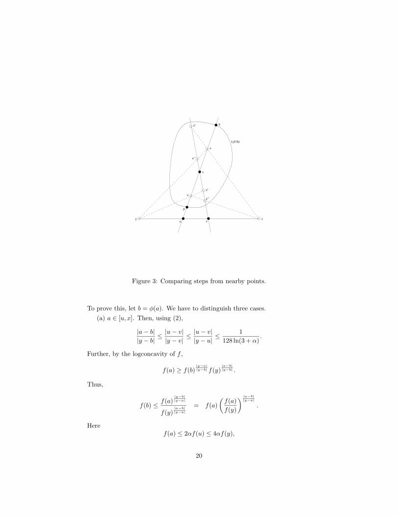
Next, we compare the function values along the lines `(u, x) and `(v, x). LetF denote the maximum value of f along `(u, x), and let p, q be the intersectionpoints of `(u, x) with the boundary of L(F/8), so that q is in the same directionfrom p as x is from u. Since x ∈ A, we know that
|u− p|, |u− q| ≤ 32|x− u|. (4)
For each point a ∈ `(u, x) we define two points a′, a′′ ∈ `(v, x) as follows. Ifa is on the semiline of `(u, x) starting from x containing u, then we obtain a′
by projecting a from y to `(v, x), and we obtain a′′ by projecting a from z. If ais on the complementary semiline, then the other way around, we obtain a′ byprojecting from z and a′′ by projecting from y.
Simple geometry shows that if
|a− u| < |y − u||u− v| |x− u|, |z − u|
|u− v| |x− u|,
then a′, a′′ exist and a′′ is between v and a′. Furthermore, a 7→ a′ and a 7→ a′′
are monotone mappings in this range.A key observation is that if |a− u| ≤ 32|x− u|, then
f(a′) < 2f(a). (5)
19
u
L(F/8)
x
a’
a’’
a’’
a’
z y
p
q
a
a
v
Figure 3: Comparing steps from nearby points.
To prove this, let b = φ(a). We have to distinguish three cases.(a) a ∈ [u, x]. Then, using (2),
|a− b||y − b| ≤
|u− v||y − v| ≤
|u− v||y − u| ≤
1128 ln(3 + α)
.
Further, by the logconcavity of f ,
f(a) ≥ f(b)|y−a||y−b| f(y)
|a−b||y−b| .
Thus,
f(b) ≤ f(a)|y−b||y−a|
f(y)|a−b||y−a|
= f(a)(
f(a)f(y)
) |a−b||y−a|
.
Heref(a) ≤ 2αf(u) ≤ 4αf(y),
20
since x ∈ A2. Thus
f(b) ≤ f(a)(4α)1
128 ln(3+α) < 2f(a).
(b) a ∈ `+(x, u). By Menelaus’ theorem,
|a− b||b− z| =
|x− a||x− u| ·
|u− v||v − z| .
By (4), |x− a|/|x− u| ≤ 16, and so by (3),
|a− b||b− z| ≤ 16df (u, v) ≤ 1
4 ln(3 + α).
By logconcavity,f(a) ≥ f(b)|a−z|/|b−z|f(z)|a−b|/|b−z|
Rewriting, we get
f(b) ≤ f(a)|b−z|/|a−z|
f(z)|a−b|/|a−z| = f(a)(
f(a)f(z)
)|a−b|/|a−z|
≤ f(a)(4α)1
4 ln(3+α)−1 ≤ 2f(a).
(c) a ∈ `+(u, x). By Menelaus’ theorem again,
|a− b||b− y| =
|x− a||x− u| ·
|u− v||v − y| .
Again by (4), |x− a|/|x− u| ≤ 16. Hence, using (2) again,
|a− b||b− z| ≤ 16df (u, v) ≤ 1
4 ln(3 + α).
By logconcavity,f(a) ≥ f(b)|a−y|/|b−y|f(z)|a−b|/|b−y|
Rewriting, we get
f(b) ≤ f(a)|b−y|/|a−y|
f(y)|a−b|/|a−y| = f(a)(
f(a)f(y)
)|a−b|/|a−y|
≤ f(a)(4α)1
4 ln(3+α)−1 ≤ 2f(a).
This proves inequality (5).Similar argument shows that if |a− u| ≤ 32|x− u|, then
f(a′′) >12f(a). (6)
Let a ∈ `(u, x) be a point with f(a) = F . Then a ∈ [p, q], and hence|a− u| < max{|p− u|, |q − u|} ≤ 32|x− u| (since x ∈ A).
21
These considerations describe the behavior of f along `(v, x) quite well. Letr = p′ and s = q′. (5) implies that f(r), f(r) ≤ F/4. On the other hand,f(a′′) > F/2 by (6).
Next we argue that a′′ ∈ [r, s]. To this end, consider also the point b ∈`(u, x) defined by b′ = a′′. It is easy to see that such a b exists and that bis between u and a. This implies that |b − u| < 32|x − u|, and so by (5),f(b) > f(b′)/2 = f(a′′)/2. Thus f(b) > F/4, which implies that b ∈ [p, q], andso b′ ∈ [p′, q′] = [r, s].
Thus f assumes a value at least F/2 in the interval [r, s] and drops to atmost F/4 at the ends. Let c be the point where f attains its maximum alongthe line `(v, x). It follows that c ∈ [r, s] and so c = d′ for some d ∈ [p, q]. Henceby (5), f(c) ≤ 2f(b) ≤ 2F . Thus we know that the maximum value F ′ of falong `(v, x) satisfies
12F ≤ F ′ ≤ 2F. (7)
Having dealt with the function values, we also need an estimate of the lengthof [r, s]:
|r − s| ≤ 2|x− v||x− u| |p− q|. (8)
To prove this, assume e.g. that the order of the points along `(u, x) isp, u, x, q (the other cases are similar). By Menelaus’ theorem,
|x− r||v − r| =
|u− y||v − y| ·
|x− p||u− p| =
(1− |v − u|
|v − y|) |x− p||u− p| .
Using (2), it follows that
|x− r||v − r| ≥
3132|x− p||u− p| .
Thus,
|x− v||v − r| =
|x− r||v − r| − 1 ≥ 31
32|x− p||u− p| − 1
=|x− u||u− p| −
132|x− p||u− p|
=|x− u||u− p|
(1− 1
32|x− p||x− u|
)
>|x− u||u− p|
(1− 1
32· 16
)=
12|x− u||u− p| .
In the last line above, we have used (4). Hence,
|v − r| < 2|x− v||x− u| |u− p|. (9)
22
Similarly,
|v − s| < 2|x− v||x− u| |u− q|.
Adding these two inequalities proves (8).Now Claim 2 follows easily. We have
µ(`(u, x)) ≥ F
8|p− q|,
while we know by Lemma 3.10(a) that
µ(`(v, x)) ≤ 2f [r, s].
By (7) and (8),
f(r, s) ≤ 2F |r − s| ≤ 4F |p− q| |x− v||x− u| ,
and hence
µ(`(v, x)) < 32|x− v||x− u|µ(`(u, x)),
proving Claim 2.Using Claims 1 and 2, we get for any A′ ⊂ A,
Pv(A′) =2
nπn
∫
A′
f(x) dx
µf (v, x)|x− v|n−1
≥ 232nπn
∫
A′
|x− u|f(x) dx
µf (u, x)|x− v|n
≥√
δ
32nπn
∫
A′
f(x) dx
µf (u, x)|x− u|n−1
≥√
δ
32Pu(A′).
This concludes the proof of Lemma 6.4. ¤
7 Proof of the isoperimetric inequality.
Let hi be the characteristic function of Si for i = 1, 2, 3, and let h4 be theconstant function 1 on K. We want to prove that
dK(S1, S2)(∫
fh2
)(∫fh2
)≤
(∫fh3
)(∫fh4
).
Let a, b ∈ K and g be a nonnegative linear function on [0, 1]. Set v(t) =(1− t)a + tb, and
Ji =∫ 1
0
hi(v(t))f(v(t))gn−1(v(t)) dt.
23
By Theorem 2.7 of [11], it is enough to prove that
dK(S1, S2)J1 · J2 ≤ J3 · J4. (10)
A standard argument [10, 13] shows that it suffices to prove the inequality forthe case when J1, J2, J3 are integrals over the intervals [0, u1], [u2, 1] and (u1, u2)respectively (0 < u1 < u2 < 1).
Consider the points ci = (1−ui)a+uib. Since ci ∈ Si, we have dK(c1, c2) ≥ ε.It is easy to see that
dK(c1, c2) ≤ (a : u2 : u1 : b)
whileJ3 · J4
J1 · J2= (a : u2 : u1 : b)f .
Thus (10) follows from Lemma 4.2.
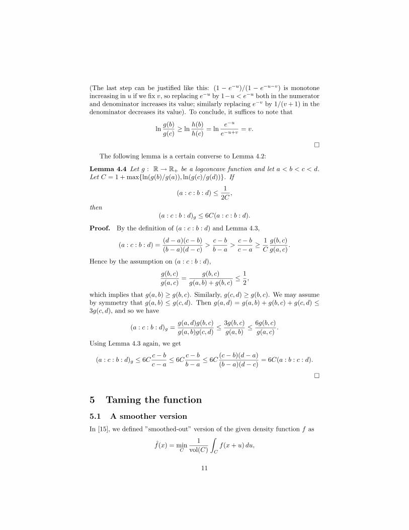
8 Proof of the mixing bound.
Let K = S1 ∪ S2 be a partition into measurable sets with πf (S1), πf (S2) > ε.We will prove that
∫
S1
Pu(S2) dπf ≥ r
218√
nR(πf (S1)− ε)(πf (S2)− ε) (11)
We can read the left hand side as follows: we select a random point X fromdistribution π and make one step to get Y . What is the probability that X ∈ S1
and Y ∈ S2? It is well known that this quantity remains the same if S1 and S2
are interchanged.For i ∈ {1, 2}, let
S′i = {x ∈ Si : Px(S3−i) <1
1000δ(x),
S′3 = K \ S′1 \ S′2.
First, suppose that πf (S′1) ≤ πf (S1)/2. Then the left hand side of (11) is atleast
11000
∫
u∈S1\S′1
f(u)f(u)
f(u) du =1
1000πf (S1 \ S′1) ≥
12000
πf (S1).
Lemma 5.3 implies that
πf (S1) ≥ πf (S1)− ε/4.
Hence, ∫
S1
Pu(S2) dπf ≥ 12000
(πf (S1)− ε
4)
which implies (11).
24
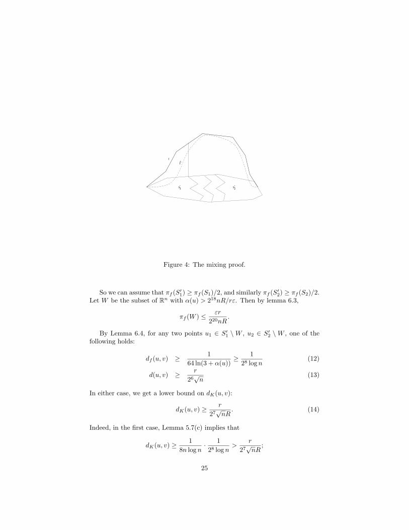
f
’’1S 2S
f
Figure 4: The mixing proof.
So we can assume that πf (S′1) ≥ πf (S1)/2, and similarly πf (S′2) ≥ πf (S2)/2.Let W be the subset of Rn with α(u) > 218nR/rε. Then by lemma 6.3,
πf (W ) ≤ εr
220nR.
By Lemma 6.4, for any two points u1 ∈ S′1 \ W , u2 ∈ S′2 \ W , one of thefollowing holds:
df (u, v) ≥ 164 ln(3 + α(u))
≥ 128 log n
(12)
d(u, v) ≥ r
26√
n(13)
In either case, we get a lower bound on dK(u, v):
dK(u, v) ≥ r
27√
nR. (14)
Indeed, in the first case, Lemma 5.7(c) implies that
dK(u, v) ≥ 18n log n
· 128 log n
>r
27√
nR;
25
in the second, Lemma 5.7(b) implies that
dK(u, v) ≥ 12R
· r
26√
n=
r
27√
nR.
Applying Theorem 2.2 to f , we get
πf (S′3) ≥r
27√
nRπf (S′1 \W )πf (S′2 \W ) ≥ r
27√
nR(πf (S1)− ε
2)(πf (S2)− ε
2).
Therefore,∫
S1
Pu(S2) dπf ≥ 12
∫
S′3
f(u)1000f(u)
f(u)du− πf (W )
≥ 12000
πf (S′3)− πf (W )
≥ r
218√
nR(πf (S1)− ε)(πf (S2)− ε)
and (11) is proved.By Corollary 1.5 in [14] it follows that for all m ≥ 0, and every measurable
set S,
|σm(S)− πf (S)| ≤ 2ε + exp(− mr2
242nR2
),
which proves Theorem 2.1.
References
[1] D. Applegate and R. Kannan (1990): Sampling and integration of nearlog-concave functions, Proc. 23th ACM STOC, 156–163.
[2] J. Bourgain: Random points in isotropic convex sets, in: Convex geomet-ric analysis (Berkeley, CA, 1996), 53–58, Math. Sci. Res. Inst. Publ., 34,Cambridge Univ. Press, 1999.
[3] A. Dinghas: Uber eine Klasse superadditiver Mengenfunktionale vonBrunn–Minkowski–Lusternik-schem Typus, Math. Zeitschr. 68 (1957),111–125.
[4] M. Dyer, A. Frieze and R. Kannan: A random polynomial time algorithmfor estimating volumes of convex bodies, Proc. 21st Annual ACM Symp.on the Theory of Computing (1989), 375–381.
[5] M. Dyer, A. Frieze and L. Stougie: talk at the Math. Prog. Symp., AnnArbor, Mich. (1994).
[6] A. Frieze, R. Kannan and N. Polson: Sampling from log-concave distribu-tions, Ann. Appl. Probab. 4 (1994), 812–837; Correction: Sampling fromlog-concave distributions, ibid. 4 (1994), 1255.
26
[7] A. Frieze and R. Kannan: Log-Sobolev inequalities and sampling from log-concave distributions, To appear in the Annals of Applied Probability
[8] A. Kalai and S. Vempala: Efficient algorithms for universal portfolios, in:Proc. 41st Annual IEEE Symp. on the Foundations of Computer Science(2000), 486-491.
[9] R. Kannan and L. Lovasz: A logarithmic Cheeger inequality and mixingin random walks, in: Proc. 31st Annual ACM STOC (1999), 282-287.
[10] R. Kannan, L. Lovasz and M. Simonovits, “Random walks and an O∗(n5)volume algorithm for convex bodies,” Random Structures and Algorithms11 (1997), 1-50.
[11] R. Kannan, L. Lovasz and M. Simonovits: “Isoperimetric problems forconvex bodies and a localization lemma,” J. Discr. Comput. Geom. 13(1995) 541–559.
[12] L. Lovasz (1992): How to compute the volume? Jber. d. Dt. Math.-Verein,Jubilaumstagung 1990, B. G. Teubner, Stuttgart, 138–151.
[13] L. Lovasz: Hit-and-run mixes fast, Math. Prog. 86 (1998), 443-461.
[14] L. Lovasz and M. Simonovits: Random walks in a convex body and animproved volume algorithm, Random Structures and Alg. 4 (1993), 359–412.
[15] L. Lovasz and S. Vempala: The geometry of logconcave functions and anO∗(n3) sampling algorithm.
[16] A. Prekopa: On logarithmic concave measures and functions, Acta Sci.Math. Szeged 34 (1973), 335-343.
[17] A. Prekopa: Stochastic Programming, Akademiai Kiado, Budapest andKluwer, Dordrecht 1995.
[18] M. Rudelson: Random vectors in the isotropic position, J. Funct. Anal.164 (1999), 60–72.
[19] R.L. Smith (1984), Efficient Monte-Carlo procedures for generating pointsuniformly distributed over bounded regions, Operations Res. 32, 1296–1308.
[20] Z.B. Zabinsky, R.L. Smith, J.F. McDonald, H.E. Romeijn and D.E. Kauf-man: Improving hit-and-run for global optimization, J. Global Optim. 3(1993), 171–192.
27