HILIGT, Upper Limit Servers I - Overview?

Saxton, R.D.a, Konig, O.b, Descalzo, M.c, Belanger, G.d, Kretschmar, P.d, Gabriel, C.d,e, Evans, P.A.f, Ibarra, A.g, Colomo, E.a,Sarmiento, M.h, Salgado, J.g, Agrafojo, A.g, Kuulkers, E.i

aTelespazio U.K. Ltd. for the European Space Agency (ESA), European Space Astronomy Centre (ESAC), Camino Bajo del Castillo s/n, 28692 Villanueva de laCanada, Madrid, Spain

bDr. Karl-Remeis-Sternwarte and Erlangen Centre for Astroparticle Physics, Friedrich-Alexander-Universitat Erlangen-Nurnberg, Sternwartstr. 7, 96049Bamberg, Germany

cDepartment of Electrical Engineering, Technical University of Denmark (DTU), Ørsteds Plads 326, 2800 Kongens Lyngby, DenmarkdEuropean Space Agency (ESA), European Space Astronomy Centre (ESAC), Camino Bajo del Castillo s/n, 28692 Villanueva de la Canada, Madrid, Spain

eCommittee on Space Research (COSPAR) – 2, place Maurice Quentin, 75039 Paris Cedex 01, FrancefUniversity of Leicester, X-ray and Observational Astronomy Group, School of Physics and Astronomy, University Road, Leicester, LE17RH, UK

gQUASAR Science Resources for the European Space Agency (ESA), European Space Astronomy Centre (ESAC), Camino Bajo del Castillo s/n, 28692 Villanuevade la Canada, Madrid, Spain

hAurora Technology B.V for the European Space Agency (ESA), European Space Astronomy Centre (ESAC), Camino Bajo del Castillo s/n, 28692 Villanueva de laCanada, Madrid, Spain

iEuropean Space Agency (ESA), European Space Research and Technology Centre (ESTEC), Keplerlaan 1, 2201 AZ Noordwijk, The Netherlands

Abstract

The advent of all-sky facilities, such as the Neil Gehrels Swift observatory, the All Sky Automated Search for Supernovae (ASAS-SN), eROSITA and Gaia has led to a new appreciation of the importance of transient sources in solving outstanding astrophysicalquestions. Identification and catalogue cross-matching of transients has been eased over the last two decades by the Virtual Obser-vatory but we still lack a client capable of providing a seamless, self-consistent, analysis of all observations made of a particularobject by current and historical facilities. HILIGT is a web-based interface which polls individual servers written for XMM-Newton,INTEGRAL and other missions, to find the fluxes, or upper limits, from all observations made of a given target. These measurementsare displayed as a table or a time series plot, which may be downloaded in a variety of formats. HILIGT currently works with datafrom X-ray and Gamma-ray observatories.

Keywords: Catalogs, Surveys, X-rays: general, Instrumentation: detectors, Upper limit, Aperture photometry

1. Introduction

Since the first discovery of X-ray emission from SCO X-1in 1962 by the Aerobee 150 sounding rocket (Giacconi et al.,1962), X-ray telescopes have been flown on satellites on a reg-ular basis. Their observations provide a record of the flux emit-ted from the brightest sources which now stretches back for 50years. Detected sources from the majority of these missions areprovided in specific catalogues (e.g. Evans et al., 2010; Webbet al., 2020; Evans et al., 2020) or are served by the compre-hensive multi-mission archive hosted at HEASARC (HeasarcTeam, 1995)1. Many missions have also left a legacy of sky im-ages. These allow upper limits to fluxes to be found from skypositions where a source has not been detected and catalogued.

As new sources are detected, due to the introduction of moresensitive instruments or because they have transitioned into abrighter state, it is of interest to know how previous observa-tions of that position on the sky can constrain the history of theflux. For known sources, while targeted observations are often

?http://xmmuls.esac.esa.int/hiligt

Email address: richard.saxton@sciops.esa.int (Saxton, R.D.)1https://heasarc.gsfc.nasa.gov/

covered by catalogues, serendipitous non-detections and detec-tions of lower flux may not be. To fully exploit the datasets ofall X-ray missions, functionality is needed capable of returningcatalogue values or of calculating upper limits from images. Inthis way, historical light curves can be generated using the fulldataset of each mission.

To this end a suite of flux / upper-limit servers have beenwritten, one for each mission, which run in parallel and eitherforward on results from the best available on-line catalogue oranalyse the images and return upper limits from a given position(Fig. 1).

In this paper we review the design and describe the inputparameters and the fields returned by each server. A compan-ion paper (Konig et al. 2021; hereafter Paper II) describesin detail how each individual server has been constructed. Abrief summary of the missions which are currently supportedis given in Table 1. Results are returned as a RepresentationalState Transfer (REST) service which may be called by any suit-able client; a web client with plotting facilities has been pro-duced and is described in detail in Sect. 2.3. The collection ofservers and the web client together are called the HIgh-energyLIght curve GeneraTor (HILIGT) which replaces an earlier up-per limit server hosted at the XMM-Newton science operations

Preprint submitted to Astronomy and Computing November 30, 2021

arX

iv:2

111.

1423

8v1

[as

tro-

ph.H

E]

28

Nov

202

1

centre (SOC) that worked exclusively with XMM-Newton data2.

2. Mission count rate and flux servers

The fundamental property measured by a photon countingdetector is the background-subtracted count rate. This can beconverted into an energy flux by convolving with the efficiencyand spectral resolution of the detector as a function of energyand by assuming a spectral model.

Each HILIGT server either returns the source count rate anderror with the equivalent flux derived from the input spectralmodel, or calculates the upper limit on the source count rate,at a user-selectable 1,2 or 3-σ level, with the equivalent upperlimit on the flux.

To enable fluxes to be compared between missions a standardset of energy bands have been defined: 0.2–2 keV (soft), 2–12keV (hard) and 0.2–12 keV (total). The one current exception isINTEGRAL which uses the three bands 20–40, 40–60 and 60–100 keV. These ranges have been set as a compromise basedon the actual energy bands of the mission instrumentation (seeTable 1).

The processing flow of a server is given in Fig. 2 and consistsof the following steps.

• Find all observations which contain a given set of equa-torial coordinates (RA, Dec). Ultimately this is done bysearching a database for image footprints which containthe sky position. The derivation of the footprints for eachmission is described in Paper II and the comparison ismade using the pgsphere package3, which is in some cases,for example for the XMM-Newton slew and pointed data,provided by a Table Access Protocol (TAP; Dowler et al.,2019) call.

• Get catalogue entries for this position. Catalogue fields,principally the source count rate and error, are accessedby making a TAP call 4 for XMM-Newton pointed data orby using the w3Browse facility provided at HEASARC5. Cross-matching with catalogues is carried out using aradius which takes into account the systematic positionalerror of the given catalogue and the likelihood of sourceconfusion. Specific details are given in Paper II, Section3.10.

• Calculate an upper limit for the sky position in imageswhere a catalogue entry is not available, using aperturephotometry.

This calculation relies on knowledge of the instrument vi-gnetting and the Point Spread Function (PSF) which is

2A comprehensive upper limit server dedicated to the XMM-Newton EPICcameras called FLIX is available at https://www.ledas.ac.uk/flix/

flix.html3https://pgsphere.github.io4http://nxsa.esac.esa.int/tap-server/tap5https://heasarc.gsfc.nasa.gov/W3Browse/w3browse-help.

html. An alternative approach would have been to use the HEASARC TAPservice.

used to calculate the encircled energy function (EEF; thefraction of counts which lie within the extraction region).In order to provide a practical distinction between a de-tection and a non-detection, a decision has been taken toreturn a flux if the background-subtracted count rate is ≥ 2times the error and otherwise return an upper limit at auser-selectable confidence level of 1, 2 or 3 sigma. Theupper limit calculation uses Bayesian statistics based onthe algorithm given in Kraft et al. (1991). We give a de-scription of this calculation in Paper II.

• Calculate the flux from the count rate. This is doneby multiplying by a factor, based on a provided spec-tral model. While in practise the spectral model ofan astrophysical object can be very complicated, forsimplicity in passing parameters, the model is cur-rently limited to either a power-law with index, Γ =

0.5, 1.0, 1.5, 1.7, 2.0, 2.5, 3.0, 3.5, or a black-body of tem-perature kT = 60, 100, 300, 1000 eV, attenuated by a neu-tral absorber of column, NH = 1 × 1020, 3 × 1020, 1 × 1021

cm−2. These values sample the typical observed spectra ofsources and include the spectrum used to calculate fluxesin the XMM-Newton catalogue (Γ = 1.7, NH = 3 × 1020

cm−2, which is based on the average X-ray spectrum ofan AGN (e.g. Turner and Pounds, 1989)). Conversion fac-tors have been hard-coded into the server software for ef-ficiency and were originally calculated using the PIMMSpackage (Mukai, 1993) or inferred from the relevant lit-erature (Forman et al., 1978; Kaluzienski, 1977; Warwicket al., 1981; Wood et al., 1984; Nugent et al., 1983).

An alternative approach would be to pre-calculate and storefluxes for each catalogued source, for each spectral model, andmake them available to HILIGT through a TAP server. Whilethis would result in a performance improvement it would proverather inflexible, as updates would be needed if the default spec-tral models were changed or if our understanding of the instru-ment calibration changed. It would also be unviable should thesystem be updated to allow the user to choose a spectral modelon-the-fly.

2.1. Inter-mission cross-calibration

Significant community effort is put into the cross-calibrationof X-ray detectors by the International Astronomical Consor-tium for High-Energy Calibration (IACHEC; Sembay et al.,2010). Recent missions, such as XMM-Newton, Swift, NuSTAR,SUZAKU and Chandra are found to return consistent fluxes towithin 10–15% (Madsen et al., 2017a). For the older missions,the factors to convert count rate into flux tend to be based on ob-servations of the Crab nebula (see Paper II), which has a power-law spectrum of Γ = 2.1. Fluxes are then only strictly valid forsimilar spectral shapes and furthermore the Crab flux and spec-tral shape are known to vary at the level of a few percent (Mad-sen et al., 2017b). To compensate for this, in the returned fluxfor these missions a systematic error of magnitude 30% (Vela5B), 15% (Ariel V), 20% (HEAO-1) and 20% (Uhuru) is addedin quadrature to the statistical error.

2

Table 1: Currently supported missions

Mission Instrument(s) modesa Data sourceb Period Energy rangec

(year) (keV)

VELA 5B ASM survey CAT 1969-1979 3–12Uhuru survey CAT 1970-1973 2–20Ariel-V ASM, SSI survey CAT 1974-1980 2–18Heao-1 A1 pointed CAT 1977-1979 0.25–25Einstein IPC, HRI pointed CAT, UL 1978-1981 0.15–4.0EXOSAT LE, ME slew, pointed CAT, UL 1983-1986 0.05–50.0Ginga LAC pointed CAT 1987-1991 1.5–30ROSAT PSPC, HRI survey, pointed CAT, UL 1990-1998 0.1–2.4ASCA GIS, SIS pointed CAT 1993-2000 0.4–12INTEGRAL ISGRI pointed UL 2000-2021+ 20–100XMM-Newton EPIC-pn slew, pointed CAT, UL 2000-2021+ 0.2–12Swift XRT pointed UL 2005-2021+ 0.2–10.0

a Missions operate in survey, slew and/or pointed observation mode.b Data source can be CATalogue and/or calculated Upper Limit (UL).c Full energy range of the instrumentation.

Image store

Mission AServer

RequestRA, DEC,…

Catalogue TAP call

HILIGTclient

TableCSVText

Latex

Light Curve

Image store

Catalogue REST call

Catalogue

REST call

External client

Request

Result (JSON,CSV,text)

Mission BServer

Mission CServer

Figure 1: Information flow between servers and clients.

Start

Find list of observations

TAP server /Dbase Table

TAP call /SQL query

Does cat entry exist?

Get catalogue entries

Source Catalogue

More Observat

ions?

Calculate upper limit

Image store

Return results

End

YesNo

Yes

No

Ra, Dec, Label

Obsid, Ra, Dec

Obsid

Figure 2: Flowchart of the design of a mission flux / upper limit server.

3

As technology has improved, there has been a tendency forthe sensitivity of missions to increase and the beam size to de-crease. This leads to quite different levels of output betweenthe missions, e.g. Vela 5B has data for 99 sources, while theXMM-Newton point source catalogue contains almost 900,000sources. A summary of the sky coverage and number of cata-logued sources is given in Paper II (Table 1).

2.2. Input / output parameters

A definition of the input parameters accepted by the serveris given in Table 2. As a minimum, a server needs to receivethe coordinates of a sky position. A default spectral model ofa power-law of spectral slope, Γ = 2, absorbed by a column ofneutral hydrogen of 3 × 1020 cm−2 is used for flux conversionand two-sigma upper limits are returned by default.

Note that for a meaningful comparison of flux between differ-ent missions it is essential that the spectral model used for theflux conversion is an accurate representation of the spectrumof the source in question. The wrong spectral model can arti-ficially introduce strong apparent variability between missions(e.g. Page, 2015).

The server can be made to ignore catalogue values and recal-culate results by setting the parameter usecat=NO.

Each mission server returns a Javascript Object Notation(JSON) structure containing the full set of fields described inTable 3, or comma-separated values (CSV) or text records con-taining a reduced, easy to display, output structure. The outputfields contain the count rate, number of source counts, numberof background counts, exposure time, flux calculated using thesupplied model and ancillary information.

Count rates returned by the instrumentation, which as can beseen from Table1 may be recorded over differing energy ranges(e.g. 0.3–2 keV and 2–10 keV for the Swift-XRT telescope)are converted into fluxes in the standard bands. Upper limitsare available for all missions which have produced a databaseof images that can be analysed. Upper limits have been pre-calculated for the INTEGRAL Soft Gamma-ray Imager (IS-GRI) and stored in a database table (see Paper II).

2.3. Clients

Servers may be hosted anywhere, although they are currentlyall located at the European Space Astronomy Centre (ESAC)6

and for convenience have been made accessible via a singleREST call:http://xmmuls.esac.esa.int/ULSservice_

passthru?MISSION=<mission>&ra=<ra>&dec=<dec>

See Table 2 for the full set of input parameters. Any servercompliant with the input and output parameters detailed inTables 2 and 3 could be added.

An example terminal client written in Python is available fordownload from:

6Note that the Swift-XRT server forwards the request onto a further serverhosted within the Leicester Database & Archive Service (LEDAS) which actu-ally makes the calculation.

http://xmmuls.esac.esa.int/hiligt/scripts/

hiligt.py

In addition an interactive, web-based client written inJavascript is available at:http://xmmuls.esac.esa.int/hiligt

The entry page of the web client (Fig. 3) allows sky positionsto be entered as a coordinate pair, a target name, to be resolvedby SIMBAD, or a text file containing a list of coordinates. Themissions to be interrogated can be selected from the upper panel(Fig. 3). Standard energy bands, the spectral model for conver-sion of count rate to flux, the confidence level of the upper limitand whether to use catalogue values, may all be selected.

The web client returns a basic output page of results for eachsource position and mission, listing the observation date, countrate and fluxes for each observation and selected energy-band(Fig. 4). By clicking on ”Advanced Settings” further fields maybe selected for display from a top panel. From the output pagethe results may be saved into a text file, a csv file or downloadedinto a LATEX table ready to be inserted into a paper. A basic lightcurve plotting function, based on the ZingChart v2.8.6 tool7,may be invoked from the output page. Alternatively, a Pythoncode to plot the results with greater flexibility may be used.8

3. Scientific Uses

HILIGT lends itself to long timescale variability analysis, tothe search for transients and to broad-band spectral variabilityanalysis. We briefly describe an example of each below.

3.1. Analysis of long-term light curvesThe first quasar to be identified was 3C 273 in 1963

(Schmidt, 1963). This was first observed in X-rays by the satel-lite Uhuru in 1970 and has subsequently been a scientific orcalibration target of all the major X-ray observatories, result-ing in a rich dataset which covers its activity over the last 50years. In Fig. 5 we show the time series of the 2–12 keV fluxfrom 3C 273 observed between 1970 and 2020, extending thework of Soldi et al. (2008) who concentrated on observationstaken between 1985 and 2006. The light curve is quite sta-ble, having maintained a mean 2–12 keV flux of 1.0×10−10 ergs−1cm−2 over the 50 year span (45 years in the source restframe;z=0.158) with a peak-to-peak variation of a factor 4. We notethat the minimum flux of 5.5 × 10−11erg s−1cm−2 was recordedon 2019-07-02 being ∼ 20% fainter than the previous minimumregistered in July 2015 (Kalita et al., 2017). This long time se-ries gives confidence that fluxes from old and new missions cansensibly be compared despite the widely differing beam sizesof the instrumentation.

3.2. Transient searchTo know whether a new X-ray source is an interesting tran-

sient it is necessary to compare the measured flux with previousdetections or upper limits. It is straightforward to write a script

7http://www.zingchart.com8http://xmmuls.esac.esa.int/hiligt/scripts/lightcurve.py

4

Figure 3: Input page for the HILIGT web client. Clicking on a mission selects it for processing, turning it from grey to bold white.

5

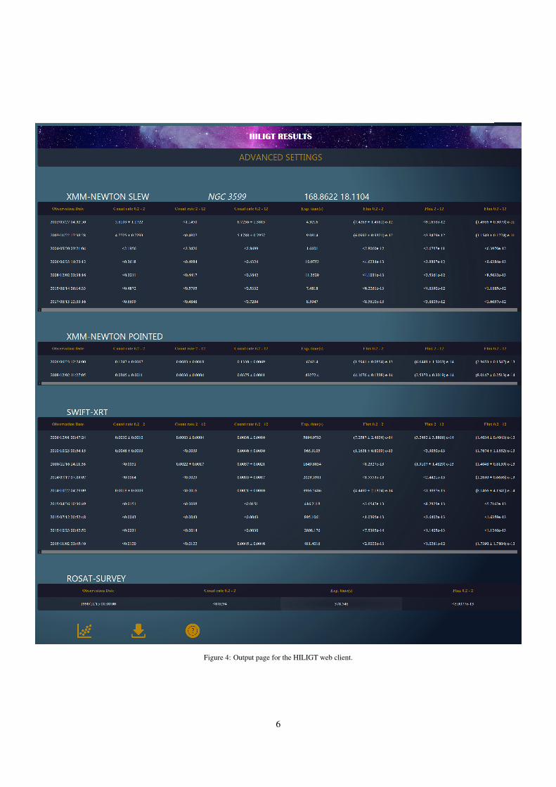
Figure 4: Output page for the HILIGT web client.

6

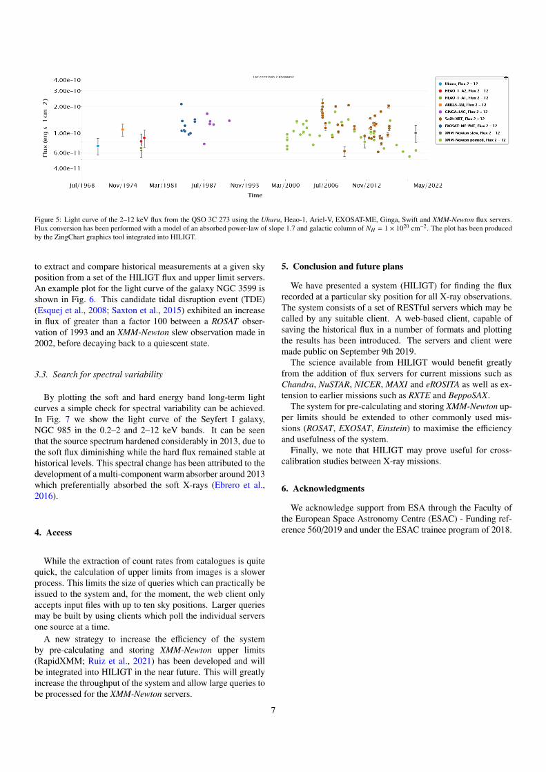
Figure 5: Light curve of the 2–12 keV flux from the QSO 3C 273 using the Uhuru, Heao-1, Ariel-V, EXOSAT-ME, Ginga, Swift and XMM-Newton flux servers.Flux conversion has been performed with a model of an absorbed power-law of slope 1.7 and galactic column of NH = 1 × 1020 cm−2. The plot has been producedby the ZingChart graphics tool integrated into HILIGT.

to extract and compare historical measurements at a given skyposition from a set of the HILIGT flux and upper limit servers.An example plot for the light curve of the galaxy NGC 3599 isshown in Fig. 6. This candidate tidal disruption event (TDE)(Esquej et al., 2008; Saxton et al., 2015) exhibited an increasein flux of greater than a factor 100 between a ROSAT obser-vation of 1993 and an XMM-Newton slew observation made in2002, before decaying back to a quiescent state.

3.3. Search for spectral variability

By plotting the soft and hard energy band long-term lightcurves a simple check for spectral variability can be achieved.In Fig. 7 we show the light curve of the Seyfert I galaxy,NGC 985 in the 0.2–2 and 2–12 keV bands. It can be seenthat the source spectrum hardened considerably in 2013, due tothe soft flux diminishing while the hard flux remained stable athistorical levels. This spectral change has been attributed to thedevelopment of a multi-component warm absorber around 2013which preferentially absorbed the soft X-rays (Ebrero et al.,2016).

4. Access

While the extraction of count rates from catalogues is quitequick, the calculation of upper limits from images is a slowerprocess. This limits the size of queries which can practically beissued to the system and, for the moment, the web client onlyaccepts input files with up to ten sky positions. Larger queriesmay be built by using clients which poll the individual serversone source at a time.

A new strategy to increase the efficiency of the systemby pre-calculating and storing XMM-Newton upper limits(RapidXMM; Ruiz et al., 2021) has been developed and willbe integrated into HILIGT in the near future. This will greatlyincrease the throughput of the system and allow large queries tobe processed for the XMM-Newton servers.

5. Conclusion and future plans

We have presented a system (HILIGT) for finding the fluxrecorded at a particular sky position for all X-ray observations.The system consists of a set of RESTful servers which may becalled by any suitable client. A web-based client, capable ofsaving the historical flux in a number of formats and plottingthe results has been introduced. The servers and client weremade public on September 9th 2019.

The science available from HILIGT would benefit greatlyfrom the addition of flux servers for current missions such asChandra, NuSTAR, NICER, MAXI and eROSITA as well as ex-tension to earlier missions such as RXTE and BeppoSAX.

The system for pre-calculating and storing XMM-Newton up-per limits should be extended to other commonly used mis-sions (ROSAT, EXOSAT, Einstein) to maximise the efficiencyand usefulness of the system.

Finally, we note that HILIGT may prove useful for cross-calibration studies between X-ray missions.

6. Acknowledgments

We acknowledge support from ESA through the Faculty ofthe European Space Astronomy Centre (ESAC) - Funding ref-erence 560/2019 and under the ESAC trainee program of 2018.

7

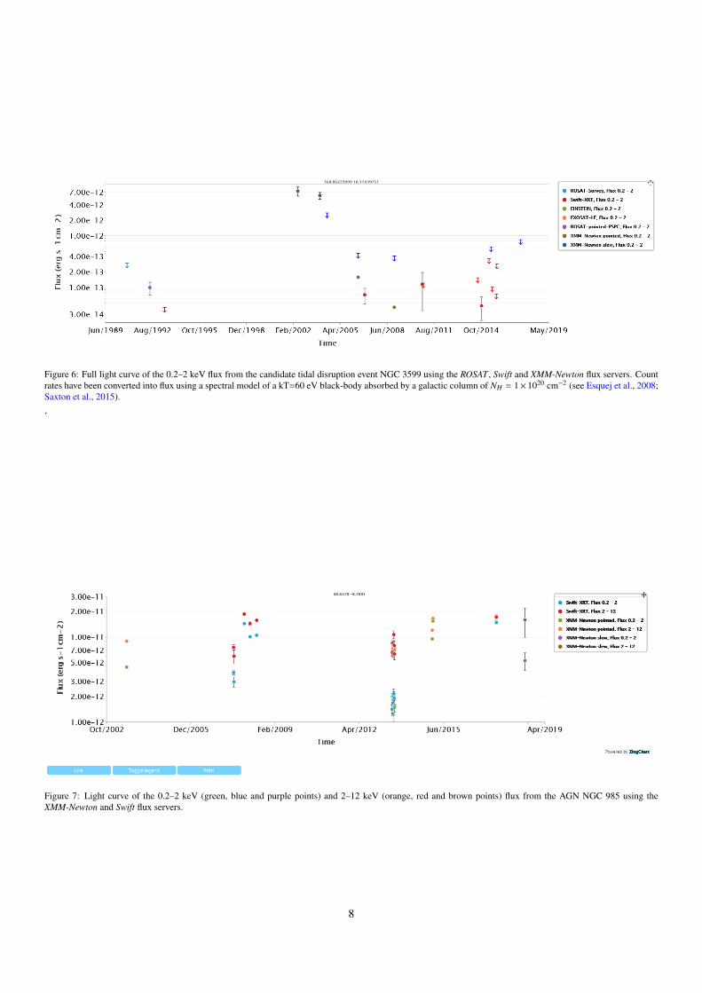
Figure 6: Full light curve of the 0.2–2 keV flux from the candidate tidal disruption event NGC 3599 using the ROSAT , Swift and XMM-Newton flux servers. Countrates have been converted into flux using a spectral model of a kT=60 eV black-body absorbed by a galactic column of NH = 1× 1020 cm−2 (see Esquej et al., 2008;Saxton et al., 2015)..

Figure 7: Light curve of the 0.2–2 keV (green, blue and purple points) and 2–12 keV (orange, red and brown points) flux from the AGN NGC 985 using theXMM-Newton and Swift flux servers.

8

References

Dowler, P., Rixon, G., Tody, D., Demleitner, M., 2019. Table Access ProtocolVersion 1.1. IVOA Recommendation 27 September 2019. URL: https://ui.adsabs.harvard.edu/abs/2019ivoa.spec.0927D.

Ebrero, J., Kriss, G.A., Kaastra, J.S., Ely, J.C., 2016. Discovery of a fast, broad,transient outflow in NGC 985. A&A 586, A72. doi:10.1051/0004-6361/201527495, arXiv:1511.07169.

Esquej, P., Saxton, R.D., Komossa, S., Read, A.M., Freyberg, M.J., Hasinger,G., Garcıa-Hernandez, D.A., Lu, H., Rodriguez Zaurın, J., Sanchez-Portal,M., Zhou, H., 2008. Evolution of tidal disruption candidates discov-ered by XMM-Newton. A&A 489, 543–554. doi:10.1051/0004-6361:200810110, arXiv:0807.4452.

Evans, I.N., Primini, F.A., Glotfelty, K.J., Anderson, C.S., Bonaventura, N.R.,Chen, J.C., Davis, J.E., Doe, S.M., Evans, J.D., Fabbiano, G., Galle, E.C.,Gibbs, Danny G., I., Grier, J.D., Hain, R.M., Hall, D.M., Harbo, P.N., He,X.H., Houck, J.C., Karovska, M., Kashyap, V.L., Lauer, J., McCollough,M.L., McDowell, J.C., Miller, J.B., Mitschang, A.W., Morgan, D.L., Moss-man, A.E., Nichols, J.S., Nowak, M.A., Plummer, D.A., Refsdal, B.L., Rots,A.H., Siemiginowska, A., Sundheim, B.A., Tibbetts, M.S., Van Stone, D.W.,Winkelman, S.L., Zografou, P., 2010. The Chandra Source Catalog. ApJS189, 37–82. doi:10.1088/0067-0049/189/1/37, arXiv:1005.4665.

Evans, P.A., Page, K.L., Osborne, J.P., Beardmore, A.P., Willingale, R., Bur-rows, D.N., Kennea, J.A., Perri, M., Capalbi, M., Tagliaferri, G., Cenko,S.B., 2020. 2SXPS: An Improved and Expanded Swift X-Ray TelescopePoint-source Catalog. ApJS 247, 54. doi:10.3847/1538-4365/ab7db9,arXiv:1911.11710.

Forman, W., Jones, C., Cominsky, L., Julien, P., Murray, S., Peters, G., Tanan-baum, H., Giacconi, R., 1978. The fourth Uhuru catalog of X-ray sources.ApJS 38, 357–412. doi:10.1086/190561.

Giacconi, R., Gursky, H., Paolini, F.R., Rossi, B.B., 1962. Evidence for xRays From Sources Outside the Solar System. Phys. Rev. Lett. 9, 439–443.doi:10.1103/PhysRevLett.9.439.

Heasarc Team, 1995. The HEASARC facility. volume 203. p. 139. doi:10.1007/978-94-011-0397-8_13.

Kalita, N., Gupta, A.C., Wiita, P.J., Dewangan, G.C., Duorah, K., 2017. Originof X-rays in the low state of the FSRQ 3C 273: evidence of inverse Comp-ton emission. MNRAS 469, 3824–3839. doi:10.1093/mnras/stx1108,arXiv:1705.02721.

Kaluzienski, L.J., 1977. Studies of Transient X-Ray Sources with the Ariel 5All-Sky Monitor. Ph.D. thesis. National Aeronautics and Space Administra-tion. Goddard Space Flight Center, Greenbelt, MD.

Kraft, R.P., Burrows, D.N., Nousek, J.A., 1991. Determination of Confi-dence Limits for Experiments with Low Numbers of Counts. ApJ 374, 344.doi:10.1086/170124.

Madsen, K.K., Beardmore, A.P., Forster, K., Guainazzi, M., Marshall,H.L., Miller, E.D., Page, K.L., Stuhlinger, M., 2017a. IACHEC Cross-calibration of Chandra, NuSTAR, Swift, Suzaku, XMM-Newton with 3C273 and PKS 2155-304. AJ 153, 2. doi:10.3847/1538-3881/153/1/2,arXiv:1609.09032.

Madsen, K.K., Forster, K., Grefenstette, B.W., Harrison, F.A., Stern, D., 2017b.Measurement of the Absolute Crab Flux with NuSTAR. ApJ 841, 56.doi:10.3847/1538-4357/aa6970, arXiv:1703.10685.

Mukai, K., 1993. PIMMS and Viewing: proposal preparation tools.Legacy vol. 3, p.21–31. URL: https://ui.adsabs.harvard.edu/abs/1993Legac...3...21M.

Nugent, J.J., Jensen, K.A., Nousek, J.A., Garmire, G.P., Mason, K.O., Walter,F.M., Bowyer, C.S., Stern, R.A., Riegler, G.R., 1983. HEAO A-2 soft X-raysource catalog. ApJS 51, 1–28. doi:10.1086/190838.

Page, M.J., 2015. X-ray photometry. MNRAS 452, L45–L48. doi:10.1093/mnrasl/slv084, arXiv:1506.07015.

Ruiz, A., Georgakakis, A., Gerakakis, S., Saxton, R., Kretschmar, P., Akylas,A., Georgantopoulos, I., 2021. The RapidXMM Upper Limit Server: X-ray aperture photometry of the XMM-Newton archival observations. arXive-prints , arXiv:2106.01687arXiv:2106.01687.

Saxton, R.D., Motta, S.E., Komossa, S., Read, A.M., 2015. Was the soft X-rayflare in NGC 3599 due to an AGN disc instability or a delayed tidal dis-ruption event? MNRAS 454, 2798–2803. doi:10.1093/mnras/stv2160,arXiv:1509.05193.

Schmidt, M., 1963. 3C 273 : A Star-Like Object with Large Red-Shift. Nature197, 1040. doi:10.1038/1971040a0.

Sembay, S., Guainazzi, M., Plucinsky, P., Nevalainen, J., 2010. Defining High-Energy Calibration Standards: IACHEC (International Astronomical Con-sortium for High-Energy Calibration), in: Comastri, A., Angelini, L., Cappi,M. (Eds.), X-ray Astronomy 2009; Present Status, Multi-Wavelength Ap-proach and Future Perspectives, pp. 593–594. doi:10.1063/1.3475350.

Soldi, S., Turler, M., Paltani, S., Aller, H.D., Aller, M.F., Burki, G.,Chernyakova, M., Lahteenmaki, A., McHardy, I.M., Robson, E.I., Staubert,R., Tornikoski, M., Walter, R., Courvoisier, T.J.L., 2008. The multi-wavelength variability of 3C 273. A&A 486, 411–425. doi:10.1051/0004-6361:200809947, arXiv:0805.3411.

Turner, T.J., Pounds, K.A., 1989. The EXOSAT spectral survey of AGN. MN-RAS 240, 833–880. doi:10.1093/mnras/240.4.833.

Warwick, R.S., Marshall, N., Fraser, G.W., Watson, M.G., Lawrence, A.,Page, C.G., Pounds, K.A., Ricketts, M.J., Sims, M.R., Smith, A., 1981.The Ariel V /3 A/ catalogue of X-ray sources. I - Sources at low galacticlatitude /absolute value of B less than 10 deg/. MNRAS 197, 865–891.doi:10.1093/mnras/197.4.865.

Webb, N.A., Coriat, M., Traulsen, I., Ballet, J., Motch, C., Carrera, F.J.,Koliopanos, F., Authier, J., de la Calle, I., Ceballos, M.T., Colomo, E.,Chuard, D., Freyberg, M., Garcia, T., Kolehmainen, M., Lamer, G., Lin, D.,Maggi, P., Michel, L., Page, C.G., Page, M.J., Perea-Calderon, J.V., Pineau,F.X., Rodriguez, P., Rosen, S.R., Santos Lleo, M., Saxton, R.D., Schwope,A., Tomas, L., Watson, M.G., Zakardjian, A., 2020. The XMM-Newtonserendipitous survey. IX. The fourth XMM-Newton serendipitous sourcecatalogue. A&A 641, A136. doi:10.1051/0004-6361/201937353,arXiv:2007.02899.

Wood, K.S., Meekins, J.F., Yentis, D.J., Smathers, H.W., McNutt, D.P., Bleach,R.D., Byram, E.T., Chupp, T.A., Friedman, H., Meidav, M., 1984. TheHEAO A-1 X-ray source catalog. ApJS 56, 507–649. doi:10.1086/190992.

9

Table 2: Input parameters of a server query.

Field Data type Units range Default Descriptionor options

mission string - - - Name of missiona

ra double precision degrees 0.0 - 360.0 - Right ascensiondec double precision degrees -90.0 - +90.0 - Declinationlabel string - - - Source nameband string - soft,hard,total,all all Energy band(s)model string - plaw,bbody plaw spectral modelspecparam float - / keV optionsb 2.0 or 100eV slope or temperaturenh float cm−2 1.0E20, 3.0E20, 1.0E21 3.0E20 Column densityulsig int sigma 1,2,3 2 Upper limit significanceusecat bool - ”yes”,”no” ”yes” Use catalogue value?FORMAT string - ”text”,”text/html”,”csv”,”JSON” ”text” Output format

a Supported missions are: XMMpnt, XMMslew, XMMStacked, RosatSurvey, RosatPointedPSPC, RosatPointedHRI, Integral, ExosatLE, Ex-osatME, Einstein, Ginga, Ariel5, Heao1, SwiftXRT, Asca, Uhuru, Vela5B.b Currently supported values are: slope=0.5,1.0,1.5,1.7,2.0,2.5,3.0,3.5 or black-body temperature=0.06,0.1,0.3,1.0 keV.

Table 3: Output fields of a server record.

Field Data type Units range Descriptionor options

start date string - - Start of obs - e.g. 2004-11-19T04:34:09end date string - - End of obs - e.g. 2004-11-19T05:47:35crate float counts / second - Count ratecrate err float counts / second - Count rate errorcrate flux float erg s−1cm−2 - Source fluxcrate flux err float erg s−1cm−2 - Error on source fluxul float counts / second - Upper limit on count rateul flux float counts / second - Upper limit of fluxulsig int - - Sigma of upper limitobsid string - - Observation identifiersrc counts int counts - Counts in source regionbck counts int counts - Counts in bckgnd regionexptime float seconds - Exposure timefilt string - - Filterimage string - - Name of imagebkgimage string - - Name of background imageexpmap string - - Name of exposure mapeef float - - Encircled energy fractionelow float keV - Lowest energy of bandehigh float keV - Highest energy of bandmission string - - Name of mission, e.g. XMM-Newtoninstrum string - - Name of instrument, e.g. EPIC-pnra double precision degrees 0.0 - 360.0 Right ascensiondec double precision degrees -90.0 - +90.0 Declinationlabel string - - Source namemodel structurea - - spectral modelstatus string - ”OK”,”NoData” status for this instrument

a This is a JSON structure containing: Column density (cm−2), spectral model (”plaw” or ”bbody”) and spectral parameter (power-law index orblack-body temperature in keV).

10