Hilbert’s Portrait via his Space-Filling Curve

Judy A. Holdener

Department of Mathematics and Statistics, Kenyon College, Gambier, OH

holdenerj@kenyon.edu

Abstract

This paper reports on how I created a 3D-printed portrait of the mathematician David Hilbert using the sixth iterate

of Hilbert’s space-filling curve. I render the portrait by varying the thickness of sequential segments of Hilbert’s

curve according to the grayscale pixel values of a well-known photo of him.

Figure 1: Hilbert’s image is embedded within his famous space-filling curve.

Bridges 2020 Conference Proceedings

231

Introduction

David Hilbert (1862–1943) was a German mathematician who was undoubtedly the most famous

mathematician of his day. Known for the 23 problems he presented at the International Congress of

Mathematics in Paris in 1900, he influenced the trajectory of mathematics in the decades to follow. A gifted

leader, Hilbert was in a good position to define the future of mathematics because he was well-versed in a

wide range of mathematical fields, having made highly original contributions to logic, geometry, analysis

and algebra. His impact is apparent to us today by the numerous mathematical objects and theorems that

now bear his name: Hilbert axioms, Hilbert space, Hilbert’s Finite Basis Theorem, and Hilbert’s curve, to

name a few.

In this paper I present a portrait I created of David Hilbert using his well-known space-filling curve

and a 3D printer. (See Figure 1.) The portrait serves as an homage to Hilbert, but it also illustrates the

human brain’s remarkable ability to fill in missing information as it works to make sense of the data received

from the surrounding world. While viewing the portrait, the reader is encouraged to experiment by squinting

and varying the viewing distance. Unlike most images, this one becomes clearer when moved further away.

Hilbert’s Space-Filling Curve

In 1879 German mathematician Eugen Netto proved that every bijective map from the unit interval [0,1] to

the unit square [0,1]2 is necessarily discontinuous, and mathematicians naturally became interested in the

possible existence of a continuous surjective map from [0,1] to [0,1]2. It took over a decade for Italian

mathematician Giuseppe Peano to answer this question in the affirmative; he provided the first example of

a space-filling curve in 1890. Hilbert conceived of his well-known curve a year later. (See [1] and [5] for

a more thorough coverage of the rich mathematics discussed briefly here.) Today Hilbert’s space-filling

curve is the better known of the two, probably because Hilbert introduced his construction geometrically,

making it easier to imagine. As Figure 2 illustrates, Hilbert constructed his curve recursively.

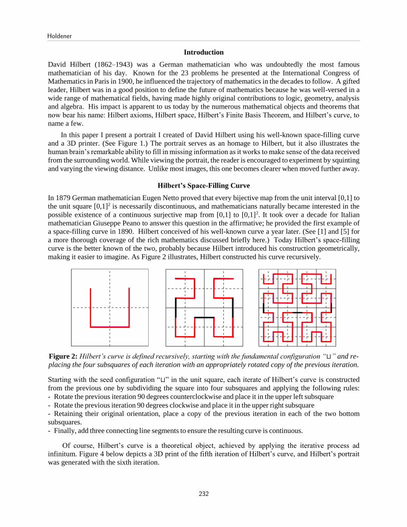
Figure 2: Hilbert’s curve is defined recursively, starting with the fundamental configuration “⊔” and re-

placing the four subsquares of each iteration with an appropriately rotated copy of the previous iteration.

Starting with the seed configuration “⊔” in the unit square, each iterate of Hilbert’s curve is constructed

from the previous one by subdividing the square into four subsquares and applying the following rules:

- Rotate the previous iteration 90 degrees counterclockwise and place it in the upper left subsquare - Rotate the previous iteration 90 degrees clockwise and place it in the upper right subsquare - Retaining their original orientation, place a copy of the previous iteration in each of the two bottom

subsquares.

- Finally, add three connecting line segments to ensure the resulting curve is continuous.

Of course, Hilbert’s curve is a theoretical object, achieved by applying the iterative process ad

infinitum. Figure 4 below depicts a 3D print of the fifth iteration of Hilbert’s curve, and Hilbert’s portrait

was generated with the sixth iteration.

Holdener

232

A Three-Phase Process

I created the portrait in the fall of 2019 while I was on sabbatical at the Institute of Computational and

Experimental Research in Mathematics (ICERM) at Brown University, participating in their special

semester on “Illustrating Mathematics.” Using Python scripts within the 3D modeling program Rhinoceros

(or “Rhino”), my code reads in an image and uses pixel data to generate a rectangular piping along the

curve. The width of the rectangular profile of the piping at a point depends on the intensity of the pixel at

that point; it is wider when the intensity of the pixel is lower (where the image is darker) and thinner when

the intensity of the pixel is higher (where the image is brighter). I chose this project with both the end

product and the creation process in mind because two of my sabbatical goals were 1) to become more

proficient programming in Python and 2) to learn how to design and print 3D mathematical objects. I broke

up the creation process into three phases.

Phase 1 – Generate square piping along the Hilbert Curve Within Rhino is a “SweepOneRail” class, which makes it easy to render a surface generated by sweeping

cross-section curves along a single rail curve. One simply draws a curve in the plane, defines the profile

shape of the (uniform) cross-section, and clicks the “SweepOneRail” button in the menu. I chose to take a

more complicated approach in generating the square piping along Hilbert’s curve, however, because

ultimately I would need to generate piping having nonuniform cross sections (that is, rectangles of varying

dimensions), and I would need to sweep the piping along thousands of curve segments. So in preparation

for phase 2, I wrote a Python script to automate the piping process. The program generates square piping

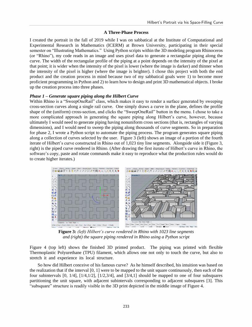
along a collection of curves selected by the user. Figure 3 (left) shows an image of a portion of the fourth

iterate of Hilbert’s curve constructed in Rhino out of 1,023 tiny line segments. Alongside side it (Figure 3,

right) is the piped curve rendered in Rhino. (After drawing the first iterate of Hilbert’s curve in Rhino, the

software’s copy, paste and rotate commands make it easy to reproduce what the production rules would do

to create higher iterates.)

Figure 3: (left) Hilbert’s curve rendered in Rhino with 1023 line segments

and (right) the square piping rendered in Rhino using a Python script

Figure 4 (top left) shows the finished 3D printed product. The piping was printed with flexible

Thermoplastic Polyurethane (TPU) filament, which allows one not only to touch the curve, but also to

stretch it and experience its local structure.

So how did Hilbert conceive of his famous curve? As he himself described, his intuition was based on

the realization that if the interval [0, 1] were to be mapped to the unit square continuously, then each of the

four subintervals [0, 1/4], [1/4,1/2], [1/2,3/4], and [3/4,1] should be mapped to one of four subsquares

partitioning the unit square, with adjacent subintervals corresponding to adjacent subsquares [3]. This

“subsquare” structure is readily visible in the 3D print depicted in the middle image of Figure 4.

Hilbert’s Portrait via his Space-Filling Curve

233

Figure 4: Stretching the piped Hilbert curve 3D printed in the more flexible

Thermoplastic Polyurethane (TPU) filament reveals local structure of the curve.

Phase 2 – Adapt the Python script to allow for rectangular piping with variable width In this next phase of the project, I constructed iterates of Hilbert’s curve using circular arcs at the curve’s

corners to smooth out the corners of the piping. Adapting the script used to create the square piping in Phase

1, I generated rectangular piping with varying width by incorporating Rhino’s “GlobalShapeBlending”

property. Given a rectangle defining the cross section of the pipe at the start of a rail curve and a second

rectangle (of different dimensions) defining the cross section at the end of the same curve, the

“GlobalShapeBlending” property allows one to create a pipe having cross sections with dimensions that

vary linearly between the two rectangles. To test my code (which, again, automates the piping process on

a selected collection of curves), I generated rectangular piping on 600+ tiny line segments and circular arcs

making up the fourth iterate of Hilbert’s curve, defining the dimensions 𝑤 (width) and ℎ (height) of the

rectangular cross sections at the endpoints (𝑥, 𝑦) of each of the curve segments by:

𝑤(𝑥, 𝑦) = 2 + 1.4 (⌊𝑥 + 𝑦⌋ mod 3) ℎ(𝑥, 𝑦) = 2

(The origin is at the bottom left-hand corner, and ⌊𝑥 + 𝑦⌋ denotes the floor function applied to 𝑥 + 𝑦.) The

top down view of the resulting surface mesh rendered by Rhino is surprisingly appealing!

Figure 5: The mesh generated by Rhino produced “Hilbert’s Intestines.”

Holdener

234

Phase 3 – Incorporate Python script to read in pixel data from an image In the final phase of this project I created Hilbert’s portrait using the sixth iterate of his curve by adapting

the script from Phase 2 so that it could read in pixel data from a given image. I constructed the portrait in

pieces by rendering 16 “subsquares” in Rhino and then printing them on an Ultimaker 3. Similar to the

piping that generated “Hilbert’s Intestines,” the width of the piping along each tiny curve segment of a

given subsquare varied linearly along the curve between the starting and ending rectangular cross sections.

Of course, the final result is necessarily of low dimension because of the lengthy printing time.

However, I did experiment within Rhino, generating Hilbert’s portrait using the seventh iterate of the space-

filling curve. The portrait’s precision increases with the use of higher iterates. (In fact, higher iterates

almost look too much like the original photograph. I appreciate the ambiguity of the current version.)

Additionally, precision within a fixed iterate increases when scaling down the image. The thumbnail of

Figure 1 provided in Figure 8 below illustrates this phenomenon. In this smaller, scaled-down version,

Hilbert’s mustache is now visible—and maybe even a hint of his glasses.

Figure 6: One of the sixteen subsquares

printing on an Ultimaker 3

In rendering Hilbert’s portrait, the dimensions, 𝑤 and

ℎ, of the rectangular cross section at (𝑥, 𝑦) depended on the

pixel data of the underlying photograph of Hilbert. Because

the piped curve would be printed ultimately in black filament

and placed on a white background, darker areas in the

photograph correspond to wider rectangular piping. The

rectangular cross sections are thinner wherever the photo is

lighter. I used the Rhino plug-in “Rhinoscript” to access

image data. The “GetPixel” command gets the color of a

pixel and “GetBrightness” computes its intensity. The height

of the piping remained fixed throughout.

This was a time-consuming endeavor, requiring be-

tween 45 to 100 minutes of printing time for each of the 16

sub-squares (see Figure 6), and there were many failed

attempts with clogged printer heads and broken filaments.

Each printed subsquare is approximately 5 inches in width,

so the entire portrait is approximately 20 × 20 inches. I glued

the 16 successful fourth iterate prints onto white foam board

to create the final portrait. (See Figure 7 for close-up views.)

Figure 7: Close-ups reveal the curve’s varying

width and its three-dimensional nature.

Figure 8: Scaling down the portrait in

Figure 1 seems to improve precision.

Hilbert’s Portrait via his Space-Filling Curve

235

Related Work and Future Directions

Creating a portrait out of a single path is not new. Bob Bosch created a number of them using the path of

a traveling salesman visiting dots (or cities) in a rectangular region; he starts with a collection of dots

distributed to have a density reflecting the shadows and highlights of a given source image. (See Chapter 6

of [2] for three famous Hamiltons rendered with Hamiltonian paths as well as a beautiful portrait of the

Mona Lisa.) My approach differs from Bosch’s in that my path is a space-filling curve, and I capture the

lights and darks of Hilbert’s image by varying the path’s width. In 2000, Ken Knowlton also used a space-

filling curve to render the portrait of its creator, Doug McKenna. (See “Portrait with a Single Line” [6, p.

171].) Like Bosch, Knowlton used a path with a fixed width. Printing the curve in white on a black

background, Knowlton captured McKenna’s likeness by using denser, higher iterates of the space-filling

curve in lighter regions of the source image and lower iterates in the darker regions. So, unlike Bosch,

Knowlton captured the lights and darks in McKenna’s portrait by capitalizing on the path’s self-similarity.

My approach differs from Knowlton’s in that I vary the width of a single iterate of a space-filling curve;

my approach captures Hilbert’s likeness by capitalizing on the space-filling property of the path.

My rendering of Hilbert is also reminiscent of the portraits produced by Ken Knowlton, Bob Bosch

and Robert Silver using photomosaics. In photographic mosaics or photomosaics, a source image is divided

into an array of rectangular regions, each of which is replaced with either some form of physical mosaic

material (e.g., stones, shells, dice or dominoes [2,4]), or with other photographs that match the pixel data

of the target image within that region (as in Robert Silver’s work [7]). The rectangular regions in the source

image are often matched with a finite set of mosaic materials (e.g., two full sets of Dominoes or a library

of photographs), and the resulting portrait often resembles a collage which becomes clearer as the viewing

distance increases. Similar to the photomosaics approach, the width of my piping is determined by reading

in local pixel data. However, my rendering of Hilbert does not have the look of a collage as it is created

with one single path.

In this project, the height of the rectangular piping remained fixed throughout the entirety of the space-

filling curve, but I intend to experiment in varying both the height and the width in future work. I also want

to make use of other types of space-filling curves to render future images. There are many possibilities!

Acknowledgements

This material is based upon work supported by the National Science Foundation under Grant No. DMS-

1439786 while I was in residence at the Institute for Computational and Experimental Research in

Mathematics in Providence, RI, during the Fall 2019 semester. I want to thank Henry Segerman for leading

a terrific introductory workshop on Rhino and David Dumas and Laura Taalman for teaching me almost

everything I know about 3D printing. I also want to thank Bob Bosch for his inspiring artwork.

References

[1] M. Bader. Space-Filling Curves: An Introduction with Applications in Scientific Computing.

Springer Science & Business Media, 2013.

[2] R. Bosch. Opt Art: From Mathematical Optimization to Visual Design. Princeton Univ. Press, 2019.

[3] D. Hilbert. “Über die stetige Abbildung einer Linie auf ein Flächenstück.” Mathematische Annalen,

vol. 38, 1891, pp. 459–460.

[4] K. Knowlton’s Mosaics. http://www.knowltonmosaics.com/ (accessed April 28, 2020).

[5] H. Sagan. Space-Filling Curves. Springer Science & Business Media, 1994.

[6] A. Seckel. Masters of Deception: Escher, Dali and the Artists of Optical Illusion. Sterling

Publishing Co., Inc., 2004.

[7] R. Silvers. Photomosaics. H. Holt and Co., 1997.

Holdener

236