Galois Theory and Hilbert’s Theorem 90

Lucas Lingle

August 19, 2013

Abstract

This paper is an exposition on the basic theorems of Galois Theory,up to and including the Fundamental Theorem. After building up thenecessary machinery, we also prove the modern statement of Hilbert’sTheorem 90, from which the classical form follows as a corollary. Theinitial presentation of Galois theory closely follows Emil Artin’s Algebrawith Galois Theory, while the later results can be found in J.S. Milne’sFields and Galois Theory and Lang’s Algebra.

Contents

1 Basics 11.1 Introduction to Field Extensions . . . . . . . . . . . . . . . . . . 11.2 Constructing Field Extensions . . . . . . . . . . . . . . . . . . . . 21.3 Minimal Polynomials . . . . . . . . . . . . . . . . . . . . . . . . . 4

2 Galois Theory 42.1 Splitting Fields . . . . . . . . . . . . . . . . . . . . . . . . . . . . 42.2 Automorphisms of the Splitting Field . . . . . . . . . . . . . . . 62.3 Derivative of a Polynomial: Multiple Roots . . . . . . . . . . . . 72.4 Degree of an Extension Field . . . . . . . . . . . . . . . . . . . . 92.5 Automorphism Groups of a Field . . . . . . . . . . . . . . . . . . 102.6 Fundamental Theorem of Galois Theory . . . . . . . . . . . . . . 16

3 Hilbert’s Theorem 90 20

1 Basics

1.1 Introduction to Field Extensions

Definition 1.1. If K is a subfield of a field L, we say L is an extension field ofK. The subfield K is then called a ground field with respect to L. As shorthand,we say L/K is a field extension.

1

Remark 1.2. Let F be a field. The collection of polynomials in a variable γwith coefficients in F forms a ring, and is denoted by is denoted F [γ]. Thecollection of rational functions in a variable γ with coefficients in F forms afield, and is denoted by is denoted F (γ). Note that γ may be a scalar or anindeterminate. Indeterminate variables will usually be denoted by x or X.

Definition 1.3. Suppose f(x) ∈ F [x]. To solve the equation f(x) = 0 meansto find a field extension E/F with an element α ∈ E such that f(α) = 0. Theelement α is then said to be a root of f(x).

Definition 1.4. Suppose E/F is a field extension, and α ∈ E. If there is anonzero polynomial with α as a root, we say α is algebraic over F . Otherwise,α is said to be transcendental over F .

Definition 1.5. We say h(x) is a polynomial over F if h(x) ∈ F [x]. We sayh(x) is reducible over F if there are non-unit elements f(x), g(x) ∈ F [x] suchthat h(x) = f(x)g(x). Otherwise, h(x) is said to be irreducible.

Proposition 1.6. Suppose p(x) is irreducible over F . If deg p(x) = 1, then ithas a root in F . If deg p(x) > 1, then p(x) has no roots in F .

Proof. The first case is trivial. If deg p(x) > 1, suppose for contradiction α ∈ Fis a root of p(x). Then by polynomial division we have q(x), r(x) ∈ F [x] suchthat

p(x) = (x− α)q(x) + r(x).

Then p(α) = r(α) = 0. Since deg r(x) < deg(x−α) = 1, r(x) is constant. Thusr(x) = 0, and p(x) = (x− α)q(x) is reducible. Contradiction.

1.2 Constructing Field Extensions

Remark 1.7. In general, when we refer to a ring R, it is a commutative ringunless otherwise noted.

Definition 1.8. A prime element p of a ring R is a nonzero, non-unit elementsuch that p|ab implies p|a or p|b.

Definition 1.9. If R is a ring, and I is an ideal of R, then for each z ∈ R,then notation z refers to the residue class of z in the quotient ring R/I. If p isa prime element of R, the ideal generated by p is denoted by (p).

Theorem 1.10. Let R be a principal ideal domain. If p ∈ R is a prime, thenthe quotient ring R/(p) is a field.

Proof. It suffices to show the existence of multiplicative inverses for each nonzeroelement of R/(p). If a 6= 0 then a 6≡ 0 mod p. Thus p - a. Since p is prime andwe are in a unique factorization domain, p only factors as p and 1. Hence thegreatest common divisor of p and a is 1. We can therefore find x, y ∈ R suchthat

ax+ py = 1.

Consequently, ax = 1.

2

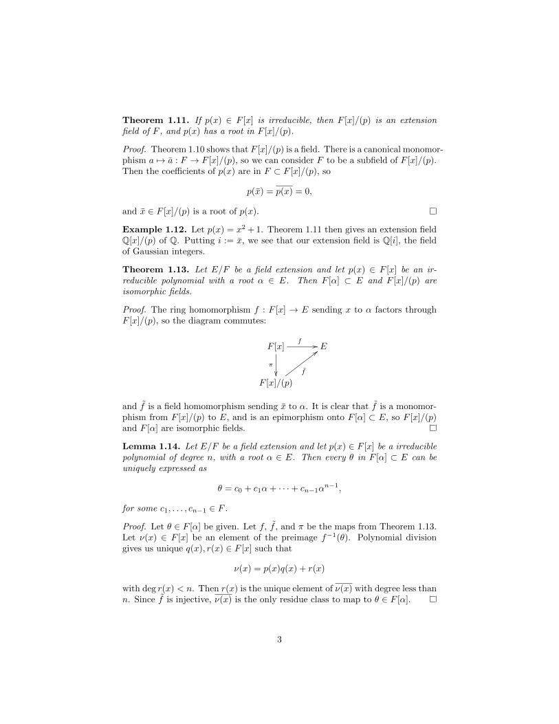
Theorem 1.11. If p(x) ∈ F [x] is irreducible, then F [x]/(p) is an extensionfield of F , and p(x) has a root in F [x]/(p).

Proof. Theorem 1.10 shows that F [x]/(p) is a field. There is a canonical monomor-phism a 7→ a : F → F [x]/(p), so we can consider F to be a subfield of F [x]/(p).Then the coefficients of p(x) are in F ⊂ F [x]/(p), so

p(x) = p(x) = 0,

and x ∈ F [x]/(p) is a root of p(x).

Example 1.12. Let p(x) = x2 + 1. Theorem 1.11 then gives an extension fieldQ[x]/(p) of Q. Putting i := x, we see that our extension field is Q[i], the fieldof Gaussian integers.

Theorem 1.13. Let E/F be a field extension and let p(x) ∈ F [x] be an ir-reducible polynomial with a root α ∈ E. Then F [α] ⊂ E and F [x]/(p) areisomorphic fields.

Proof. The ring homomorphism f : F [x] → E sending x to α factors throughF [x]/(p), so the diagram commutes:

F [x]

π

f // E

F [x]/(p)

f

;;

and f is a field homomorphism sending x to α. It is clear that f is a monomor-phism from F [x]/(p) to E, and is an epimorphism onto F [α] ⊂ E, so F [x]/(p)and F [α] are isomorphic fields.

Lemma 1.14. Let E/F be a field extension and let p(x) ∈ F [x] be a irreduciblepolynomial of degree n, with a root α ∈ E. Then every θ in F [α] ⊂ E can beuniquely expressed as

θ = c0 + c1α+ · · ·+ cn−1αn−1,

for some c1, . . . , cn−1 ∈ F .

Proof. Let θ ∈ F [α] be given. Let f, f , and π be the maps from Theorem 1.13.Let ν(x) ∈ F [x] be an element of the preimage f−1(θ). Polynomial divisiongives us unique q(x), r(x) ∈ F [x] such that

ν(x) = p(x)q(x) + r(x)

with deg r(x) < n. Then r(x) is the unique element of ν(x) with degree less thann. Since f is injective, ν(x) is the only residue class to map to θ ∈ F [α].

3

1.3 Minimal Polynomials

Definition 1.15. Let E/F be a field extension, and suppose α ∈ E is algebraicover F . Consider the collection of polynomials in F [x] which have α as a root.Among these, there will be a polynomial p(x) whose degree is less than orequal to the degrees of the others. Such a polynomial p(x) is then said to be aminimum polynomial of α.

Remark 1.16. For the remainder of this section, E/F will be a field extension,α ∈ E will be algebraic over F , and p(x) ∈ F [x] will be a minimum polynomialof α.

Lemma 1.17. The polynomials over F for which α ∈ E is a root are multiplesof the polynomial p(x).

Proof. Since p(α) = 0, any multiple of p(x) also has α as a root. Conversely,suppose f(x) ∈ F [x] and f(α) = 0. As in the proof of Proposition 1.6, polyno-mial division then shows that p(x) divides f(x).

Lemma 1.18. The polynomial p(x) is irreducible over F .

Proof. Suppose p(x) is reducible. Then there exist non-constant polynomialsf(x), g(x) ∈ F [x] such that p(x) = f(x)g(x). Then f(α)g(α) = p(α) = 0.Without loss of generality, f(α) = 0. Thus α is a root of f(x), and hence p(x)is not a minimum polynomial of α. Contradiction.

Lemma 1.19. Every polynomial irreducible over F , for which α is a root, hasthe form c · p(x) for some c ∈ F .

Definition 1.20. The monic minimum polynomial is called the minimum poly-nomial of α.

2 Galois Theory

2.1 Splitting Fields

Theorem 2.1. Suppose f(x) ∈ F [x]. Then there exists an extension field Eof F such that f(x) is the product of linear factors with coefficients in E. It isthen said that f(x) splits in E.

Proof. The polynomial f(x) possesses a unique factorization into irreduciblefactors over F . Thus we may write

f(x) = c(x− α1) · · · (x− αr)p1(x) · · · ps(x)

where α1, . . . , αr are roots of f(x) in F and p1(x), . . . , ps(x) are the irreduciblefactors of degree higher than 1.

If s = 0, then E = F and we are done. Otherwise, let αr+1 be a root ofp1(x). Then p1 factors in the extension field F [αr+1] ∼= F [x]/(p1), via

p1(x) = (x− αr+1)q1(x).

4

Now take F [αr+1] as the ground field, and factor f(x) in F [αr+1]. This newfactorization will include at least one additional linear factor, and possibly more.If f(x) splits in F [αr+1], we are done. If not, we can repeat the procedure. Aftera finite number of iterations, we obtain an extension field

E := F [αr+1, . . . , αn] = F [α1, . . . , αn]

in which f(x) can be factored into linear terms.

Theorem 2.2. Let f(x) be a polynomial over F , and Ω be an extension fieldof F in which f(x) can be split into linear factors

f(x) = c(x− α1) · · · (x− αn).

The smallest subfield of Ω in which f(x) splits is the field E obtained by themethod in Theorem 2.1.

Proof. If there is a field M , between F and Ω, in which f(x) splits, then Mmust contain α1, . . . , αn. Then M ⊃ F [α1, . . . , αn]. Thus E := F [α1, . . . , αn] isthe smallest field in which f(x) splits.

Remark 2.3. The field E is called the splitting field of f(x) between F andΩ. But if we have a distinct field extension Ω′/F in which f(x) splits, thenthe splitting field of f(x) between F and Ω′ may be different as well. But howdifferent? Not very.

Theorem 2.4. Let f(x) be a polynomial over F , and let Ω and Ω′ be twoextension fields of F in which f(x) splits. Then the splitting fields of f(x)between Ω and F and between Ω′ and F are isomorphic.

Remark 2.5. The above theorem allows us to speak of the splitting field off(x) ∈ F [x], i.e., the smallest extension field of F in which f(x) in which splits.We will prove this theorem in a more general form:

Theorem 2.6. Suppose F and F are isomorphic. Suppose f(x) ∈ F [x], and

let f(x) be the corresponding polynomial over F . Assume Ω/F and Ω/F arefield extensions in which f(x) and f(x) split, respectively. Let E be the splitting

field of f(x) between Ω and F . Let E be defined analogously for f(x). The

isomorphism between F and F can then be extended to an isomorphism betweenE and E.

Proof. Factoring f(x) ∈ F [x] in Ω, we obtain

f(x) = (x− α1) · · · (x− αn).

And factoring f(x) ∈ F [x] in Ω, we have

f(x) = (x− α1) · · · (x− αn).

Theorem 2.2 then shows that E := F [α1, . . . , αn] and E := F [α1, . . . , αn].

Clearly F ∼= F , so we have F [x]/(f) ∼= F [x]/(f), and hence F [α1] ∼= F [α1].

Induction then shows that F [α1, . . . , αn] ∼= F [α1, . . . , αn].

5

2.2 Automorphisms of the Splitting Field

Remark 2.7. Let F be a field, and E be the splitting field for f(x) over F .What are all the automorphisms of E which leave F fixed pointwise? A partialanswer follows immediately from Theorem 2.6:

Lemma 2.8. Suppose f(x) possesses a nonlinear irreducible factor with dis-tinct roots α1, . . . αn ∈ E. Then for each i 6= j, Theorem 1.13 tells us thereis a canonical isomorphism from F [αi] to F [αj ], and by Theorem 2.6 this iso-morphism can be extended to give a nontrivial automorphism of E which fixesF ⊂ E pointwise.

Definition 2.9. Let E/F be a field extension. The set of all automorphismsof E will be denoted by Aut(E). The set of all automorphisms of E which fixF pointwise will be denoted by Aut(E/F ).

Theorem 2.10. Factor f(x) into irreducible polynomials over F :

f(x) = c(x− α1) · · · (x− αr)p1(x) · · · ps(x),

where the pi(x) are factors of degree higher than 1. If

1. E is the splitting field of f(x) over F, and

2. no linear factor appears more than once in the splitting of pi(x) in E,(i.e., pi(x) has no multiple roots in E) for i = 1, . . . , n,

then the collection of elements in E which are fixed pointwise by Aut(E/F ) isprecisely F .

Proof. Let deg f(x) = n, and let r be the number of linear terms in the fac-torization above. We will induct by showing that if the theorem is true forr = k + 1, then it is true for r = k. For our base case, suppose r = n. We thensee that E = F and the theorem is trivially true. For the induction hypothesis,we assume the theorem holds for r = k + 1.

Now suppose f(x) has k linear factors. If αk+1 is a root of p1(x), the fieldF can be extended to the field F [αk+1] in which f(x) has at least k + 1 linearfactors. To derive the factorization in F [αk+1], we first factor f(x) as in thestatement of this theorem, and then proceed to further factor each pi(x) overthe field F [αk+1]. We obtain a factorization

f(x) = c(x− α1) · · · (x− αr)(x− β1) · · · (x− βµ)q1(x) · · · qν(x),

where each qk(x) is a irreducible polynomial of degree greater than 1, obtainedfrom the factorization of some pi(x). Note that

1. E is still the splitting field of f(x) over F [αk+1], and

2. None of the qk(x) have any repeated factors in E, since otherwise somepi(x) would have have repeated factors in E, (which would contradict thesecond supposition of the theorem.)

6

Then by the induction hypothesis we know that if θ ∈ E is left fixed byAut(E/F [αk+1]), then θ ∈ F [αk+1].

Now suppose that θ ∈ E remains fixed by Aut(E/F ). Then since

Aut(E/F [αk+1]) ⊂ Aut(E/F ),

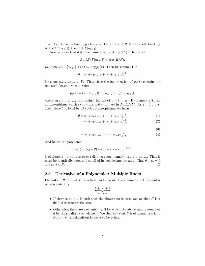
we know θ ∈ F [αk+1]. Set t := deg p1(x). Then by Lemma 1.14,

θ = c0 + c1αk+1 + · · ·+ ct−1αt−1k+1

for some c0, . . . , ct−1 ∈ F . Then since the factorization of p1(x) contains norepeated factors, we can write

p1(x) = (x− αk+1)(x− αk+2) · · · (x− αk+t),

where αk+1, . . . , αk+t are distinct factors of p1(x) in E. By Lemma 2.8, theautomorphisms which swap αk+1 and αk+j , are in Aut(E/F ), for j = 2, . . . , t.Then since θ is fixed by all such automorphisms, we have

θ = c0 + c1αk+1 + · · ·+ ct−1αt−1k+1 (1)

= c0 + c1αk+2 + · · ·+ ct−1αt−1k+2 (2)

... (3)

= c0 + c1αk+t + · · ·+ ct−1αt−1k+t (4)

And hence the polynomial

ψ(x) = (c0 − θ) + c1x+ · · ·+ ct−1xt−1

is of degree t− 1 but possesses t distinct roots, namely, αk+1, . . . , αk+t. Thus itmust be identically zero, and so all of its coefficients are zero. Thus θ − c0 = 0and so θ ∈ F .

2.3 Derivative of a Polynomial: Multiple Roots

Definition 2.11. Let F be a field, and consider the summation of the multi-plicative identity

1 + · · ·+ 1︸ ︷︷ ︸n times

• If there is no n ∈ N such that the above sum is zero, we say that F is afield of characteristic zero.

• Otherwise, there are elements n ∈ N for which the above sum is zero. Letd be the smallest such element. We then say that F is of characteristic d.Note that this definition forces d to be prime.

7

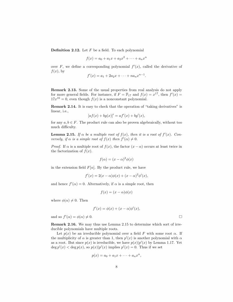
Definition 2.12. Let F be a field. To each polynomial

f(x) = a0 + a1x+ a2x2 + · · ·+ anx

n

over F , we define a corresponding polynomial f ′(x), called the derivative off(x), by

f ′(x) = a1 + 2a2x+ · · ·+ nanxn−1.

Remark 2.13. Some of the usual properties from real analysis do not applyfor more general fields. For instance, if F = F17 and f(x) = x17, then f ′(x) =17x16 = 0, even though f(x) is a nonconstant polynomial.

Remark 2.14. It is easy to check that the operation of “taking derivatives” islinear, i.e.,

[af(x) + bg(x)]′ = af ′(x) + bg′(x),

for any a, b ∈ F . The product rule can also be proven algebraically, without toomuch difficulty.

Lemma 2.15. If α be a multiple root of f(x), then it is a root of f ′(x). Con-versely, if α is a simple root of f(x) then f ′(α) 6= 0.

Proof. If α is a multiple root of f(x), the factor (x−α) occurs at least twice inthe factorization of f(x).

f(α) = (x− α)2φ(x)

in the extension field F [α]. By the product rule, we have

f ′(x) = 2(x− α)φ(x) + (x− α)2φ′(x),

and hence f ′(α) = 0. Alternatively, if α is a simple root, then

f(x) = (x− α)φ(x)

where φ(α) 6= 0. Then

f ′(x) = φ(x) + (x− α)φ′(x),

and so f ′(α) = φ(α) 6= 0.

Remark 2.16. We may thus use Lemma 2.15 to determine which sort of irre-ducible polynomials have multiple roots.

Let p(x) be an irreducible polynomial over a field F with some root α. Ifthe multiplicity of α is greater than 1, then p′(x) is another polynomial with αas a root. But since p(x) is irreducible, we have p(x)|p′(x) by Lemma 1.17. Yetdeg p′(x) < deg p(x), so p(x)|p′(x) implies p′(x) = 0. Thus if we set

p(x) = a0 + a1x+ · · ·+ anxn,

8

where an 6= 0, then

p′(x) = a1 + 2a2x+ · · ·+ nanxn−1.

Consequently, p(x) can have multiple roots only if a1 = 2a2 = · · · = nan = 0.But an 6= 0, so if F is of characteristic zero, nan 6= 0.

Corollary 2.17. An irreducible polynomial over a field of characteristic zerocan only have simple roots.

2.4 Degree of an Extension Field

Definition 2.18. Let E/F be a field extension; the field E is a vector spaceover F . The dimension of this vector space is called the degree of the extensionE/F , and is denoted by [E : F ]. If the dimension is infinite, the degree of theextension is said to be infinite as well.

Lemma 2.19. Let p(x) be an irreducible polynomial in F , with some root α.Put n = deg p(x). The extension field E = F [α] possesses the generators

1, α, α2, . . . , αn−1,

and these generators form a basis of E over F . Consequently, [E : F ] = n.

Proof. By Lemma 1.14, 1, α, α2, . . . , αn−1 is a spanning set of E over F . Ifthis set were linearly dependent, then p(x) would be of a higher degree thanthe minimum polynomial m(x) of α. By Lemma 1.17, p(x) would be a non-constant multiple of m(x), contrary to the irreducibility of p(x). Consequently,1, α, α2, . . . , αn−1 is a basis of E over F , and [E : F ] = n.

Theorem 2.20. Let F be a ground field, E be an extension of F , and Ω be anextension of E; Ω ⊃ E ⊃ F . Then [Ω : E][E : F ] = [Ω : F ].

Proof. Let ω1, . . . , ωn be a basis of E/F , and Ω1, . . . ,Ωm be a basis of Ω/E.Every θ ∈ Ω can be written as a linear combination

θ = α1Ω1 + · · ·+ αmΩm,

with the αi ∈ E. Each αi is likewise a linear combination over F :

αi = ai1ω1 + · · ·+ ainωn.

Consequently,

θ =

m∑i=1

[ n∑j=1

aijωj

]Ωi =

m∑i=1

n∑j=1

aijωjΩi, (5)

so the elements ωjΩi ∈ Ω are nm generators of Ω with respect to F . It is appar-ent that the generators form a spanning set of Ω. To prove linear independence,

9

set θ = 0. Then the bracketed terms in (5) are each equal to zero, since the Ωi’sare linearly independent over E. We obtain

ai1ω1 + · · ·+ ainωn = 0

for i = 1, 2, . . . ,m. Since the ωj ’s are linearly independent over F , each aij = 0,and the proof is complete.

Proposition 2.21. If [E : F ] = 1, then E = F .

Proof. If the degree of E/F is one, then E is generated by any element of Fwhich is linearly independent (i.e., is nonzero). Since 1 is nonzero, every elementof E is in F . Then E = F .

Corollary 2.22. If Ω ⊃ E ⊃ F and [E : F ] = [Ω : F ], then Ω = E.

Proof. By Theorem 2.20, [Ω : E][E : F ] = [Ω : F ]. Since [E : F ] = [Ω : F ], thisimplies [Ω : E] = 1 and by Proposition 2.21, Ω = E.

2.5 Automorphism Groups of a Field

Theorem 2.23. Let E be a field and σ1, . . . , σn be distinct automorphisms ofE. Then if c1, . . . , cn ∈ E and

c1σ1(x) + · · ·+ cnσn(x) = 0

for all x ∈ E, then follows that c1 = · · · = cn = 0.

Proof. Assume for contradiction’s sake that there is a nontrivial relation amongthe σi. Suppose there are r nonzero coefficients in this relation. Without lossof generality, let this relation be among the first r of the σi. In other words,suppose there exist c1, . . . , cr ∈ E, all nonzero, such that

c1σ1(x) + · · ·+ crσr(x) = 0, (6)

for all x ∈ G. Clearly, r 6= 1, since c1σ1(x) = 0 implies c1 = c1σ1(1) = 0,contrary to our assumption that each ci 6= 0. Thus r > 1.

Since Equation (6) holds for every x ∈ G, it holds even if we replace x withax. Thus

c1σ1(a)σ1(x) + · · ·+ crσr(a)σr(x) = 0. (7)

Now multiply Equation (6) by σr(a), and subtract the result from (7). Weobtain

c1[σ1(a)− σr(a)]σ1(x) + · · ·+ cr−1[σr−1(a)− σr(a)]σr−1(x) = 0, (8)

which is shorter than Equation (6). If it can be shown that not all of thesecoefficients are zero, this will contradict the assumption that r is least and wewill be done.

Since σ1(x) and σr(x) are distinct functions, their values differ at someelement of G. Assume the value of a we picked earlier was such an element.Then σ1(a) − σr(a) 6= 0. Since c1 6= 0, we know c1[σ1(a) − σr(a)] 6= 0, and soEquation (8) is a nontrivial relation shorter than Equation (6).

10

Lemma 2.24. Suppose σ1, . . . , σn are n distinct automorphisms of E. Thesubset F ⊂ E of elements fixed pointwise by this collection of automorphismsforms a field. F is then called the fixed field of σ1 . . . , σn.

Proof. It is only necessary to show the closure of F with respect to addition,subtraction, multiplication, and division. For each a, b ∈ F ,

σi(a± b) = σi(a)± σi(b) = a± b,

and likewise for multiplication and division.

Theorem 2.25. If F is the fixed field of n distinct automorphisms σ1, . . . , σn ofE, then [E : F ] ≥ n.

Proof. Assume for contradiction’s sake that [E : F ] = r < n, and let ω1, . . . , ωrbe a basis of E/F . Then for each θ ∈ E, we have some c1, . . . , cr ∈ F such that

θ = c1ω1 + · · ·+ crωr. (9)

The system ξ1σ1(ω1) + ξ2σ2(ω1) + · · ·+ ξnσn(ω1) = 0

...

ξ1σ1(ωr) + ξ2σ2(ωr) + · · ·+ ξnσn(ωr) = 0

(10)

of r linear equations in n unknowns, n > r, has a nontrivial solution ξ1, · · · , ξn ∈E. For each i, multiply the i-th of equation of (10) by ci ∈ F . Since each ci isin the fixed field of each σj , we have σj(ci) = ci for each i. Thus we obtain asystem

ξ1σ1(c1ω1) + ξ2σ2(c1ω1) + · · ·+ ξnσn(c1ω1) = 0...

ξ1σ1(crωr) + ξ2σ2(crωr) + · · ·+ ξnσn(crωr) = 0.

(11)

Adding together the left sides of (11), we have

ξ1σ1(θ) + · · ·+ ξnσn(θ) = 0,

where ξ1, · · · , ξn are not all zero, and where θ, given by (9), is any arbitraryelement of E. This contradicts Theorem 2.23, so [E : F ] = r ≥ n.

Example 2.26. Take E = Q(x), the field of rational functions with rationalcoefficients, and consider the following automorphisms of Q(x):

f(x) 7→ f(x), f

(1

x

), f(1− x), f

(1

1− x

), f

(x

x− 1

), f

(x− 1

x

). (12)

Note that these automorphisms form a group. Denote by F the fixed field ofthis group. By Theorem 2.25, [E : F ] ≥ 6. What are the elements of F? It iseasy to verify that

J(x) =(x2 − x+ 1)3

x2(x− 1)2

11

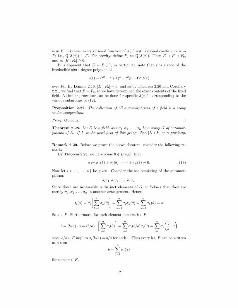
is in F . Likewise, every rational function of J(x) with rational coefficients is inF ; i.e., Q(J(x)) ⊂ F . For brevity, define F0 := Q(J(x)). Then E ⊃ F ⊃ F0,and so [E : F0] ≥ 6.

It is apparent that E = F0(x); in particular, note that x is a root of theirreducible sixth-degree polynomial

p(t) = (t2 − t+ 1)3 − t2(t− 1)2J(x)

over F0. By Lemma 2.19, [E : F0] = 6, and so by Theorem 2.20 and Corollary2.21, we find that F = F0, so we have determined the exact contents of the fixedfield. A similar procedure can be done for specific J(x)’s corresponding to thevarious subgroups of (12).

Proposition 2.27. The collection of all automorphisms of a field is a groupunder composition.

Proof. Obvious.

Theorem 2.28. Let E be a field, and σ1, σ2, . . . , σn be a group G of automor-phisms of E. If F is the fixed field of this group, then [E : F ] = n precisely.

Remark 2.29. Before we prove the above theorem, consider the following re-mark:

By Theorem 2.23, we have some θ ∈ E such that

a := σ1(θ) + σ2(θ) + · · ·+ σn(θ) 6= 0. (13)

Now let i ∈ 1, · · · , n be given. Consider the set consisting of the automor-phisms

σiσ1, σiσ2, . . . , σiσn.

Since these are necessarily n distinct elements of G, it follows that they aremerely σ1, σ2, . . . , σn in another arrangement. Hence

σi(a) = σi

[ n∑k=1

σk(θ)

]=

n∑k=1

σiσk(θ) =

n∑k=1

σk(θ) = a.

So a ∈ F . Furthermore, for each element element b ∈ F ,

b = (b/a) · a = (b/a) ·[ n∑i=1

σi(θ)

]=

n∑i=1

σi(b/a)σi(θ) =

n∑i=1

σi

(b

a· θ)

since b/a ∈ F implies σi(b/a) = b/a for each i. Thus every b ∈ F can be writtenas a sum

b =

n∑i=1

σi(γ)

for some γ ∈ E.

12

Proof of Theorem 2.28. Let α1, . . . , αm be any m elements of E. The theoremwill be proved if we can show that the αi’s are linearly dependent wheneverm > n, and hence that [E : F ] ≤ n; from Theorem 2.25 it will then follow that[E : F ] = n, and that consequently the group G contains all automorphismswhich leave F fixed.

Consider the systemx1σ1(α1) + x2σ1(α2) + · · ·+ xmσ1(αm) = 0

...

x1σn(α1) + x2σn(α2) + · · ·+ xmσn(αm) = 0

(14)

of n linear equations in m unknowns, m > n. This system has a nontrivialsolution x1, . . . , xn, with, say, x1 6= 0. Clearly λx1, . . . , λxm is also a solutionfor any λ ∈ E. Let θ be an element of E such that the a obtained by (13) isnonzero. Select λ so that λx1 = θ. Now define yj = λxj for j = 1, 2, . . . , n.Note that y1 = θ in this solution. For notational convenience, we can assumethe values of the xj ’s in our initial solution coincide with values of the yj ’s.Thus we can assume x1 = θ.

Upon applying σi to the system (14), we have

σi(x1)σiσk(α1) + σi(x2)σiσk(α2) + · · ·+ σi(xm)σiσk(αm) = 0

for k = 1, 2, . . . , n. Since σiσk (for k = 1, 2, . . . , n) are n distinct automor-phisms in G, this is the same system as (14) but where x1, . . . xm are replacedby σi(x1), . . . , σi(xm). Consequently σi(x1), . . . , σi(xm) is also a solution of(14). Now since the sum of any two solutions to a system of linear homogenousequations is itself a solution, we will define

x′j :=

n∑i=1

σi(xj),

for j = 1, 2, · · · ,m. Then x′1, x′2, . . . , x

′m is solution of (14), and we have each

x′j ∈ F by Remark 2.29. Since we have x1 = θ, the above sum for j = 1coincides with Equation (13), and hence we have x′1 = a 6= 0. Hence thesolution x′1, x

′2, · · · , x′m is nontrivial. Since the σi’s form a group, one of them is

the identity automorphism. Therefore one of the equations in (14) has the form

x′1α1 + x′2α2 + · · ·+ x′mαm = 0,

and so the αj ’s are linearly dependent over F .

Corollary 2.30. Let G = σ1, . . . , σn be a finite group of automorphisms ofE. Let F be the fixed field of G. Then every automorphism of E which fixes Fis in G; i.e., G = Aut(E/F ).

Proof. By Theorem 2.28, we know that [E : F ] = n. If there were an auto-morphism τ ∈ Aut(E/F ) such that τ /∈ G, then the subgroup H of Aut(E/F )generated by G and τ would have order greater than n. But then H has fixedfield F , and hence n = [E : F ] = |H| > n, which is absurd.

13

Theorem 2.31. Let G be a finite group of automorphisms σ1, σ2, . . . , σn of thefield E, and let F be the fixed field of G. Then any element α ∈ E is algebraicover F .

Proof. Consider σ1(α), σ2(α), . . . , σn(α). Define αi := σi(α) for i = 1, 2, . . . , n.Suppose r of these n values are unique, for some r ≤ n. Without loss of gen-erality, assume α1, α2, . . . , αr are distinct. Note than α itself is one of these,since there is some j ∈ 1, . . . , n such that σj is the identity automorphism.Then the set σiσ1(α), . . . , σiσr(α) consists of r distinct values, since the im-ages of different elements under the same automorphism are distinct. But theseare contained in the collection σiσ1(α), . . . , σiσn(α) = σ1(α), . . . σn(α), andare therefore merely the elements α1, α2, . . . , αr in another arrangement. Set

φ(x) =

r∏k=1

(x− αk).

From the remarks in the above paragraph, it follows that

σi(φ(x)) =

r∏k=1

σi(x− αk) =

r∏k=1

(x− σi(αk)) = φ(x).

Consequently, the coefficients of φ(x) are unchanged by the automorphisms inG, and so they must reside in F . But φ(x) has the roots α1, α2, . . . , αr, one ofwhich is α. Thus α is algebraic over F .

Corollary 2.32. The polynomial φ(x), defined above, is irreducible over F .

Proof. Let f(x) ∈ F [x] be any polynomial with the root α. The σi do notchange the coefficients of f(x), so

f(αi) = f(σi(α)) = σi(f(α)) = σi(0) = 0

and thus f(x) has the roots α1, α2, · · · , αr, and so deg f(x) ≥ r. Hence φ(x) isthe minimum polynomial of α, and by Lemma 1.18, φ(x) is irreducible.

Definition 2.33. If the roots of an irreducible polynomial are all simple, thenthe polynomial is said to be separable. In general, a polynomial is said to beseparable if each of its irreducible factors are separable.

Example 2.34. Consider the polynomial f(x) = x4−2 over Q. Now constructthe splitting field E by the method in Theorem 1.11. Then x4− 2 splits in E as

(x− 4√

2)(x+4√

2)(x− i 4√

2)(x+ i4√

2).

And hence E = Q( 4√

2, i 4√

2) = Q( 4√

2, i). What is the degree of the splittingfield? To begin with, we know

[E : Q] = [E : Q(4√

2)] · [Q(4√

2) : Q].

14

By Lemma 2.19, [E : Q( 4√

2)] = 2, since i ∈ E is a root the irreducible quadratic

polynomial x2 + 1 over Q( 4√

2). Lemma 2.19 also shows that

1, 4√

2, 4√

22, 4√

23

forms a basis of Q( 4√

2)/Q, so [Q( 4√

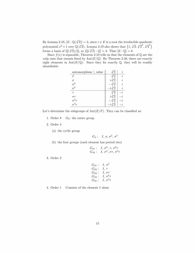
2) : Q] = 4. Thus [E : Q] = 8.Since f(x) is separable, Theorem 2.10 tells us that the elements of Q are the

only ones that remain fixed by Aut(E/Q). By Theorem 2.28, there are exactlyeight elements in Aut(E/Q). Since they fix exactly Q, they will be readilyidentifiable:

automorphism \ value 4√

2 i

I 4√

2 i

σ i 4√

2 i

σ2 − 4√

2 i

σ3 −i 4√

2 i

τ 4√

2 −iστ i 4

√2 −i

σ2τ − 4√

2 −iσ3τ −i 4

√2 −i

Let’s determine the subgroups of Aut(E/F ). They can be classified as:

1. Order 8 G8: the entire group

2. Order 4

(a) the cyclic group

G4 : I, σ, σ2, σ3

(b) the four groups (each element has period two)

G41 : I, σ2, τ, σ2τG42 : I, σ2, στ, σ3τ

3. Order 2

G21 : I, σ2

G22 : I, τG23 : I, στG24 : I, σ2τG25 : I, σ3τ

4. Order 1 Consists of the element I alone

15

The inclusion relations between the subgroups are described by the diagram

G8

G41

<<

G4

OO

G42

bb

G22

<<

G24

OO

G21

bb OO <<

G23

OO

G25

bb

I

ii bb OO << 55

The subfields of E which correspond to fixed fields of these subgroups are in-terrelated in the same manner, except that the inclusions are in the oppositedirection. Thus if N is the order of a subgroup, and K is the correspondingfixed field then [E : K] = N and hence [K : Q] = 8/N .

Remark 2.35. It should be noted that while each subgroup H of Aut(Ω/L)determines a subfield of Ω fixed by H, it is not true that each subfield of Ωcorresponds to the fixed field of some subgroup of Aut(Ω/L). For instance,Q[ 3√

2] only has the identity as an automorphism and so Q ⊂ Q[ 3√

2] is not thefixed field of some subset of the automorphism group.

Now consider Example 2.34. The field Q( 4√

2) has two automorphisms, Iand σ2. Note that this is despite having [Q( 4

√2) : Q] = 4. Note further that the

fixed field of I, σ2 is actually Q[√

2] and not Q. Hence Q doesn’t serve as thefixed field of some subgroup of Aut(Q( 4

√2)/Q) = I, σ2.

What exactly is going wrong? These fields are unwieldy; the correspondenceis only one-way, and, in the latter case, the order of the extension doesn’t seemto match the order of the automorphism group. A few definitions in the nextsection will show us exactly when field extensions behave nicely.

2.6 Fundamental Theorem of Galois Theory

Definition 2.36. A field extension E/F in which every element of E is al-gebraic over F is said to be an algebraic extension. Otherwise it is called atranscendental extension.

Definition 2.37. Let E/F be an algebraic extension.

• Suppose the minimum polynomial of every α ∈ E is separable. Then E/Fis called a separable extension. Otherwise, E/F is said to be inseparable.

• Suppose the minimum polynomial of every α ∈ E splits in E. Then E/Fis called a normal extension.

16

Remark 2.38. Suppose E/F is an algebraic extension. Then E/F is a normaland separable extension if and only if, for all α ∈ E, the minimum polynomialφ(x) of α has deg φ(x) = [F [α] : F ] distinct roots in E. (Note that the equalityof the degree of φ(x) and the degree of F [α]/F follows from Lemma 2.19.)

Definition 2.39. If E/F is a finite field extension and the fixed field of Aut(E/F )is exactly F , then E/F is said to be a Galois extension. In such a case, we sayAut(E/F ) is the Galois group of E/F , and denote it by Gal(E/F ).

Theorem 2.40. For an algebraic field extension E/F , the following are equiv-alent:

(a) E is the splitting field of some separable polynomial f(x) ∈ F [x]

(b) F is the fixed field of a finite group G of automorphisms on E

(c) E is normal, separable, and of finite degree over F

(d) E/F is a Galois extension.

Proof. (a) =⇒ (d). Let E be the splitting field of a separable polynomialf(x) ∈ F [x]. By Theorem 2.10, F is the fixed field of Aut(E/F ), and so E/Fis Galois.

(d) =⇒ (b). If E/F is a Galois extension, it is finite as per Definition 2.39.It is then clear that there can only be finitely many elements of Gal(E/F ). SoF is the fixed field of the finite group Gal(E/F ) of automorphisms on E.

(b) =⇒ (c). Let G be a finite group of automorphisms of E, and let Fbe the fixed field of G. By Theorem 2.28, we know [E : F ] = |G| and soE/F is a finite extension. Take any α ∈ E, take the orbit of α under G,and construct the polynomial φ(x) from Theorem 2.31. Recall that this is theminimum polynomial of α, and has deg φ(x) distinct factors in E. Thus byRemark 2.38, E/F is normal and separable.

(c) =⇒ (a). By the assumption that E/F is a finite extension, write E =F [α1, . . . , αn]. Let fi(x) ∈ F [x] be the minimum polynomial of αi. Then define

f(x) :=

n∏i=1

fi(x).

Then by the assumption that E/F is a normal extension, each fi(x) splits in E,so E is the splitting field of f(x). Because E/F is a separable extension, f(x)is separable.

Remark 2.41. Let E/F be a Galois extension. If F is the fixed field of afinite group G of automorphisms of E, then Theorem 2.28 shows that G has[E : F ] elements. But Theorem 2.19 also shows that Gal(E/F ) has [E : F ]elements. Because E/F finite by definition of being Galois, [E : F ] is finite, soG = Gal(E/F ).

17

Corollary 2.42. Every finite separable extension E/F is contained in a finiteGalois extension E†/F .

Proof. Let E = F [α1, . . . , αm]. Let fi(x) be the minimum polynomial of αi overF , for i = 1, . . . ,m. Define E† to be the splitting field of f(x) :=

∏fi(x). Since

E/F is a separable extension, each fi(x) is separable. Hence E† is the splittingof a separable polynomial f(x) ∈ F [x]. Theorem 2.40 tells us that E†/F istherefore a finite Galois extension.

Corollary 2.43. Let E ⊃ M ⊃ F . If E/F is a Galois extension, then so isE/M .

Proof. Theorem 2.40 tells us that E/F is a Galois extension if and only if it isthe splitting field of some separable polynomial f(x) ∈ F [x]. Since f(x) ∈M [x]is separable, E/M is Galois.

Definition 2.44. A finite extension E/F is called cyclic, abelian, ..., or solvable,if E/F is a Galois extension, and Gal(E/F ) is cyclic, abelian, ..., or solvable,respectively.

Definition 2.45. Let E be a field, and G be a group of automorphisms of E.For brevity’s sake, denote the fixed field of G by EG.

Definition 2.46. Let G be a group, and let H be a subgroup of G. The indexof H in G, denoted [G : H], is the minimum number of cosets of H such thatthe union of the cosets is G. For a finite group G, and a subgroup H of G, thisis equivalent to

[G : H] =|G||H|

.

Theorem 2.47 (The Fundamental Theorem of Galois Theory). Let E/F bea Galois extension, and set G = Gal(E/F ). The maps f : H 7→ EH andg : M 7→ Gal(E/M) are inverse bijections between

subgroups H of G ↔ intermediate fields F ⊂M ⊂ E.

Moreover,

(a) the correspondence is inclusion-reversing: H1 ⊃ H2 ⇐⇒ EH1 ⊂ EH2 .

(b) indexes equal degrees: [H1 : H2] = [EH2 : EH1 ].

(c) σHσ−1 ↔ σM , i.e., EσHσ−1

= σ(EH); Gal(E/σM) = σGal(E/M)σ−1.

(d) H is normal in G ⇐⇒ EH/F is a normal extension, in which case

Gal(EH/F ) ∼= G/H.

Proof. For the first statement, we need to show f : H 7→ EH and g : M 7→Gal(E/M) are inverse maps:

18

• Let H be a subgroup of G = Gal(E/F ). Then as noted in Remark 2.41,Gal(E/EH) = H.

• Let M be an intermediate field. Then by Corollary 2.43, E/M is Galois,and hence by Remark 2.41, EGal(E/M) = M .

And now for the rest:

(a) It is apparent that

H1 ⊃ H2 =⇒ EH1 ⊂ EH2 =⇒ Gal(E/EH1) ⊃ Gal(E/EH2).

But Gal(E/EHi) = Hi, for i = 1, 2, so

EH1 ⊂ EH2 =⇒ H1 ⊃ H2.

(b) As observed in Remark 2.41, for every subgroup H of G satisfies

[E : EH ] = |Gal(E/EH)| = [Gal(E/EH) : I] = [H : I].

The general case follows immediately, since

[H1 : I] = [H1 : H2][H2 : I] and [E : EH1 ] = [E : EH2 ][EH2 : EH1 ].

(c) Take τ ∈ H and α ∈ E. Then for every σ ∈ G,

τα = α ⇐⇒ στσ−1(σα) = σα. (15)

Suppose α ∈ EH . Then στσ−1(σα) = σα holds for all τ ∈ H. Hence

σ(EH) is fixed by every element of σHσ−1; i.e., σ(EH) ⊂ EσHσ−1

.

Now suppose that α ∈ EσHσ−1

. Then α = σ(σ−1α) is fixed by everyelement of σHσ−1. By the equivalence shown in (15) above, we have

σ−1α ∈ EH i.e., α = σ(σ−1α) ∈ σ(EH). Consequently, EσHσ−1 ⊂ σ(EH).

Therefore we have EσHσ−1

= σ(EH).

Note that for any intermediate field M , the field extension E/M is Galois.Set H := Gal(E/M). Then

EσHσ−1

= σ(EH) = σ(EGal(E/M)) = σM,

soσHσ−1 = Gal(E/EσHσ

−1

) = Gal(E/σM)

and henceσGal(E/M)σ−1 = Gal(E/σM).

19

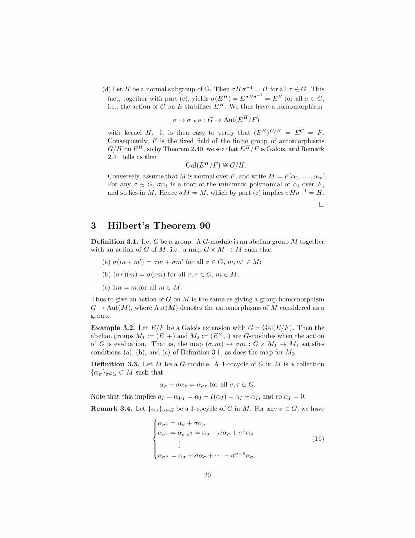
(d) Let H be a normal subgroup of G. Then σHσ−1 = H for all σ ∈ G. This

fact, together with part (c), yields σ(EH) = EσHσ−1

= EH for all σ ∈ G,i.e., the action of G on E stabilizes EH . We thus have a homomorphism

σ 7→ σ|EH : G→ Aut(EH/F )

with kernel H. It is then easy to verify that (EH)G/H = EG = F .Consequently, F is the fixed field of the finite group of automorphismsG/H on EH , so by Theorem 2.40, we see that EH/F is Galois, and Remark2.41 tells us that

Gal(EH/F ) ∼= G/H.

Conversely, assume thatM is normal over F , and writeM = F [α1, . . . , αm].For any σ ∈ G, σαi is a root of the minimum polynomial of αi over F ,and so lies in M . Hence σM = M , which by part (c) implies σHσ−1 = H.

3 Hilbert’s Theorem 90

Definition 3.1. Let G be a group. A G-module is an abelian group M togetherwith an action of G of M , i.e., a map G×M →M such that

(a) σ(m+m′) = σm+ σm′ for all σ ∈ G, m,m′ ∈M ;

(b) (στ)(m) = σ(τm) for all σ, τ ∈ G, m ∈M ;

(c) 1m = m for all m ∈M .

Thus to give an action of G on M is the same as giving a group homomorphismG→ Aut(M), where Aut(M) denotes the automorphisms of M considered as agroup.

Example 3.2. Let E/F be a Galois extension with G = Gal(E/F ). Then theabelian groups M1 := (E,+) and M2 := (E×, ·) are G-modules when the actionof G is evaluation. That is, the map (σ,m) 7→ σm : G ×M1 → M1 satisfiesconditions (a), (b), and (c) of Definition 3.1, as does the map for M2.

Definition 3.3. Let M be a G-module. A 1-cocycle of G in M is a collectionασσ∈G ⊂M such that

ασ + σατ = αστ for all σ, τ ∈ G.

Note that this implies aI = αI·I = αI + I(αI) = αI + αI , and so αI = 0.

Remark 3.4. Let ασσ∈G be a 1-cocycle of G in M . For any σ ∈ G, we haveασ2 = ασ + σασ

ασ3 = ασ·σ2 = ασ + σασ + σ2ασ...

ασn = ασ + σασ + · · ·+ σn−1ασ.

(16)

20

Thus if G = 〈σ〉 is a cyclic group of order n, a 1-cocycle of G in M is determinedby the value x := ασ ∈M . Furthermore, this x satisfies the equation

x+ σx+ · · ·+ σn−1x = 0. (17)

Conversely, if x ∈M satisfies Equation (17) then the formulas

ασi = x+ σx+ · · ·+ σi−1x (18)

define a 1-cocycle of G in M . Hence for a cyclic group G = 〈σ〉 there is abijective correspondence between

1-cocycles αττ∈G ⊂Mατ7→ασ←→ασi← [x

x ∈M satisfying (17),

where the map ασi ← [ x is shorthand for the function taking x to αττ∈G inaccordance with the formulas given by (18).

Remark 3.5. Let ασσ∈G and βσσ∈G be 1-cocycles of G in M . Then sinceασ + σατ = αστ and βσ + σβτ = βστ for all σ, τ ∈ G, we know that

(ασ + βσ) + σ(ατ + βτ ) = αστ + βστ ,

for all σ, τ ∈ G. Hence the sum of two 1-cocycles is a 1-cocycle:

ασσ∈G + βσσ∈G := ασ + βσσ∈G.

From here it is easy to see that the set of 1-cocycles of G in M form a group,which we will denote by Z1(G,M).

Definition 3.6. A 1-coboundary of G in M is a collection of elements ασσ∈Gsuch that there exists some β ∈M for which

ασ = σβ − β for every σ ∈ G.

Remark 3.7. Let ασσ∈G be a 1-coboundary. Then ασ = σβ−β, ατ = τβ−β,and αστ = στβ − β. Hence

ασ + σατ = σβ − β + σ(τβ − β) = στβ − β = αστ ,

so every 1-coboundary is a 1-cocycle.

Remark 3.8. Now if ασσ∈G and βσσ∈G are 1-coboundaries of G in M ,then there are α, β ∈M such that ασ = σα−α and βσ = σβ − β for all σ ∈ G.Consequently,

ασ + βσ = σ(α+ β)− (α+ β),

and so ασ + βσσ∈G is a 1-coboundary. It is easy to verify that the set of all1-coboundaries of G in M forms a group, which we shall denote by B1(G,M).

21

Remark 3.9. If G acts trivially on M , i.e., σm = m for all σ ∈ G and allm ∈ M , then a 1-cocycle is simply a group homomorphism, and the only 1-coboundary is identically zero.

Definition 3.10. The quotient group

H1(G,M) := Z1(G,M)/B1(G,M).

is called the first cohomology group of G in M .

Remark 3.11. An exact sequence of G-modules

0→M ′ →M →M ′′ → 0

gives rise to an exact sequence

0→M ′G →MG →M ′′

G d→ H1(G,M ′)→ H1(G,M)→ H1(G,M ′′).

Let m′′ ∈ M ′′G, and let m ∈ M map to m′′. For all σ ∈ G, σm − m lies inthe submodule M ′, and the 1-cocycle given by ασ : σ 7→ σm − m : G → M ′

represents d(m′′).

Theorem 3.12 (Modern Statement of Hilbert’s Theorem 90). Let E/F be aGalois extension, and set G = Gal(E/F ). Then H1(G,E×) = 1, i.e., every1-cocycle of G in E× is a 1-coboundary.

Proof. Let ασσ∈G be a 1-cocycle of G in E×. In multiplicative notation thismeans that

αστ = ασ · σ(ατ )

for all στ ∈ G. If ασσ∈G is a 1-coboundary, then in multiplicative notation,there is some γ ∈ E× such that ασ = σγ

γ for all σ ∈ G.

Now because the ατ are nonzero (since ασσ∈G ⊂ E×), Theorem 2.23 showsthat the following finite linear combination (finite because E/F Galois impliesG is finite) ∑

τ∈Gαττ : E → E

is not the zero map, i.e., there exists an θ ∈ E such that

β :=∑τ∈G

αττ(θ) 6= 0.

But then for each σ ∈ G,

σβ =∑τ∈G

σ(ατ )στ(θ) (19)

=∑τ∈G

α−1σ αστ · στ(θ) (20)

= α−1σ∑τ∈G

αστστ(θ) (21)

= α−1σ β (22)

22

Hence ασ = βσ(β) . Setting γ := β−1 then gives

ασ =β

σ(β)=

γ−1

σ(γ−1)=σ(γ)

γ,

and thus ασσ∈G is a 1-coboundary.

Definition 3.13. Let E/F be a Galois extension, and set G = Gal(E/F ). Letα ∈ E. The norm of α is defined to be

Nmα =∏σ∈G

σα.

Remark 3.14. For each τ ∈ G, we have

τ(Nmα) =∏σ∈G

τσα = Nmα,

and so Nmα ∈ F . Note that the norm map

α 7→ Nmα : E× → F×

is a homomorphism.

Example 3.15. The norm map for C× → R× is α 7→ αα = |α|2, and the normmap for (Q[

√d])× → Q× is a+ b

√d 7→ (a+ b

√d)(a− b

√d) = a2 − db2.

Remark 3.16. Frequently, one is interested in determining the kernel of thenorm map. It is apparent that any element of the form β

τβ has norm 1. Ournext result, the classical form of Hilbert’s Theorem 90, will show that for cyclicextensions, all elements with norm 1 are of this form.

Theorem 3.17 (Clasical Statement of Hilbert’s Theorem 90). Let E/F be afinite cyclic extension with Galois group 〈σ〉. If NmE/F α = 1 then α = β/σβ,for some β ∈ E.

Proof. Let m be the order of σ. Then the condition that α has norm 1 isequivalent to saying that

α · σα · · ·σm−1α = 1,

so by a multiplicative analogue of Remark 3.4, there is a 1-cocycle αττ∈〈σ〉of 〈σ〉 in E× with ασ = α. The modern statement of Hilbert’s Theorem 90then shows that αττ∈〈σ〉 is a 1-coboundary, and so there is a γ ∈ E such thatασ = σ(γ)/γ. Setting β := γ−1, we have

α = ασ =β

σβ,

as desired.

23

Acknowledgements

It is my pleasure to thank my mentor, Tianqi Fan, for guiding my studiesthis summer, and helping me to understand the big picture behind the ideaspresented in this paper. I would also like to thank Professor May for his feedbackon my paper, and for organizing and directing the REU program.

References

[1] Artin, Emil. Algebra with Galois Theory. American Mathematical Society.2nd Edition. 2007.

[2] Lang, Serge. Algebra. Addison-Wesley. 2nd Edition. 1984.

[3] Milne, James. Fields and Galois Theory. Online course notes. Version 4.40.Retrieved June 28th, 2013.

24