Highway to Success: The Impact of the Golden QuadrilateralProject for the Location and Performance of Indian Manufacturing

Ejaz Ghani, Arti Grover Goswami, and William R. Kerr∗, †

October 2013

Abstract

We investigate the impact of the Golden Quadrilateral (GQ) highway project on the Indian organizedmanufacturing sector using enterprise data. The GQ project upgraded the quality and width of 5,846 kmof roads in India. We use a difference-in-difference estimation strategy to compare non-nodal districts basedupon their distance from the highway system. We find several positive effects for non-nodal districts located0-10 km from the GQ network that are not present in districts 10-50 km away, most notably higher entryrates. These results are not present for districts located on another major highway system, the North-SouthEast-West corridor (NS-EW). Improvements for portions of the NS-EW system were planned to occur at thesame time as GQ but were subsequently delayed. The results also hold when using a instrumental variablesframework that draws straight lines between nodal cities. Additional tests show that the GQ project’s effectoperates in part through a stronger sorting of land-intensive industries from nodal districts to non-nodaldistricts located on the GQ network. The GQ upgrades also improved allocative effi ciency of activity forindustries initially positioned on the GQ network. The GQ upgrades further helped spread economic activityto moderate-density districts and intermediate cities.

JEL Classification : L10, L25, L26, L60, L80, L90, L91, L92, M13, O10, R00, R10, R11, R14

Keywords : Highways, roads, infrastructure, India, development, manufacturing, density, rent.

∗Author institutions and contact details: Ghani: World Bank, Eghani@worldbank.org; Grover Goswami: World Bank,agrover1@worldbank.org; Kerr: Harvard University, Bank of Finland, and NBER, wkerr@hbs.edu.†Acknowledgments: This paper is being submitted to the CEPR-PEDL grant team with respect to their generous support

of the work. It is a substantial revision of NBER Working Paper Series, No. 18524; some additional, minor revisions are stillongoing. We are grateful to Partha Mukhopadhyay, Stephen O’Connell, Hyoung Gun Wang and seminar participants for helpfulsuggestions/comments. We are particularly indebted to Sarah Elizabeth Antos and Henry Jewell for excellent data work and maps.Funding for this project was provided by a Private Enterprise Development in Low-Income Countries grant by the Centre or EconomicPolicy Research and by World Bank’s Multi-Donor Trade Trust Fund. The views expressed here are those of the authors and not ofany institution they may be associated with.

1

1 Introduction

Adequate transportation infrastructure is an essential ingredient for economic development and growth. Beyond

simply facilitating cheaper and more effi cient movements of goods, people, and ideas across places, transportation

infrastructure impacts the distribution of economic activity and development across regions, the extent to which

agglomeration economies and effi cient sorting can be realized, the levels of competition among industries and

concomitant reallocation of inputs towards productive enterprises, and much more. Rapidly expanding countries

like India and China often face severe constraints on their transportation infrastructure. Many business leaders,

policy makers, and academics describe infrastructure as a critical hurdle for sustained growth that must be met

with public funding, but to date we have a very limited understanding of the economic impact of those projects.

We study the impact of the Golden Quadrilateral (GQ) project, a large-scale highway construction and

improvement project in India. The GQ project sought to improve the connection of four major cities in India:

Delhi, Mumbai, Chennai, and Kolkata. The GQ system comprises 5,846 km (3,633 mi) of road connecting many

of the major industrial, agricultural, and cultural centers of India. It is the fifth-longest highway in the world.

The massive project began in 2001, was two-thirds complete by 2005, and mostly finished in 2007. Datta (2011),

a study that we describe in greater detail below, finds that the GQ upgrades quickly improved the inventory

management and sourcing choices of manufacturing plants located in non-nodal districts along the GQ network

by 2005.

This paper investigates the impact of the GQ highway upgrades on the organization and performance of the

organized manufacturing sector for India. We employ plant-level data from the years 1994 and 1999-2009 to study

the impact of highway infrastructure investments on Indian manufacturing. We study how proximity to GQ in

non-nodal districts affected the organization of manufacturing activity using establishment counts, employment,

and output levels, especially among newly entering plants that are making location choice decisions before or after

the upgrades. This work on the organization of the manufacturing sector also considers industry-level sorting

and the extent to which intermediate cities in India are becoming more attractive for manufacturing plants. We

study the impact for the sector’s performance through measures of average labor productivity and total factor

productivity (TFP).

Our work exploits several forms of variation to identify the effects. First, our data include surveys before

and after the upgrades, which allows us to exploit pre-post variation for the GQ upgrades. Second, we use GIS

software to code how far districts are from the GQ network. Throughout this paper, we measure effects for

nodal districts in the GQ network, but we do not ascribe a causal interpretation to these effects because the GQ

upgrades were in large part designed to improve the connections of these hubs and the GQ upgrade decision may

have been endogenous to the growth prospects of these hubs. Instead, our key focus is on non-nodal districts that

are very close to the GQ network compared to those that are farther away. We specifically compare non-nodal

districts 0-10 km from the GQ network to districts 10-50 km away (and in some specifications with additional

concentric rings to 200 km away). Additional sources of variation come from the sequence in which districts were

upgraded, differences in industry traits within the manufacturing sector, and differences in the traits of non-nodal

districts 0-10 km from the GQ network.

We find generally positive effects of the GQ upgrades on the organized manufacturing sector. Long-differenced

1

and panel estimations find substantial growth in entry rates in non-nodal districts within 10 km of the GQ network

after the GQ upgrades. These patterns are absent in districts 10-50 km away, and the data suggest that there

might have even been declines in entry rates in districts farther away (perhaps indicative of a more substantial

shift of activity towards the GQ network due to the improved connectivity). Heightened entry rates are evident in

districts where the GQ project upgraded existing highways and where the GQ project constructed new highways

where none existed before.

Beyond entry rates, we find positive impacts for the total level of manufacturing activity across all districts

within 10 km of the GQ network. These increases in aggregate activity are slower to develop than entry rates

and find their strongest expression at the very end of our sample period. The increases, especially with respect

to output, are statistically significant in long-differenced estimation forms, but the patterns are less stark than

the new entry rates. In terms of performance, we find some modest evidence of increases in labor productivity

and TFP among manufacturing plants in non-nodal districts within 10 km of the GQ network that is not present

in districts more than 50 km from the GQ system.

Beyond the variation afforded by the distance of districts from the GQ network, we undertake additional

exercises that indicate these changes in district outcomes are mostly linked to the GQ upgrades. These exercises

also address concerns regarding the endogenous placement of infrastructure that prevents a causal interpretation

of infrastructure’s role. As Duranton and Turner (2011) highlight, the endogenous placement could bias findings

in either direction. Infrastructure investments may be made to encourage development of regions with high growth

potential, which would upwardly bias measurements of economic effects that do not control for this underlying

potential. However, there are many cases where infrastructure investments are made to try to turn around

and preserve struggling regions. They may also be directed through the political process towards non-optimal

locations (i.e., “bridges to nowhere”). These latter scenarios would downward bias results.

Our first exercise is to compare districts along the GQ network to a placebo group. India has a second major

highway network called the North-South East-West (NS-EW) highway. The NS-EW highway was scheduled for

a partial upgrade at the same time as the GQ network, but this upgrade was delayed. The upgrade has since

been undertaken. Comparisons of non-nodal districts on the GQ network to non-nodal districts on the NS-EW

network are attractive given the comparable initial condition of being located on a major transportation network.

Moreover, the government intended to start upgrading the NS-EW highway network, albeit on a somewhat smaller

scale, at the same time as the GQ upgrades. We do not find similar effects along the NS-EW highway system

that we observe along the GQ highway system, which is comforting for our experimental design.

Our second exercise, which has a deeper foundation in the literature discussed below, is to implement an

instrumental variables (IV) analysis. This work instruments in the long-differenced regressions for the actual

proximity to the GQ network with the proximity of districts to straight lines between nodal cities around which

the GQ network was built. These estimations continue to confirm our results, often failing to reject the null

hypothesis that OLS and IV results are the same.

Third, we examine dynamic panel estimations. For our entry results, these dynamic models do not find a lead

effect in non-nodal districts prior to the GQ upgrades. There is then a dramatic increase in entry after the GQ

upgrades begin. These specifications suggest that the timing of the improvements in the manufacturing sector

2

is closely tied to the timing of the improvements in the GQ network. On the other hand, our analysis suggests

a much slower development process for total activity. As a second approach, we separate districts by when the

GQ upgrades were completed. Differences in coeffi cient magnitudes by implementation date are again consistent

with the economic effects that we measure being due to the GQ improvements.

Building from these exercises, we finally study the extent to which the GQ upgrades influenced the organization

of manufacturing activity. We find that the heightened entry rates following the GQ upgrades in non-nodal

districts within 10 km of the GQ network were strongest in industries that are very land and building intensive.

Interestingly, we find the opposite pattern for nodal districts, where the shift is towards industries that are less

intensive in land and buildings. These intuitive patterns are suggestive evidence that the GQ upgrades improved

the spatial allocation of activity in India, similar to improvements in within-district spatial allocation due to

infrastructure observed by Ghani et al. (2012). We also find evidence that the GQ upgrades improved the

allocative effi ciency (Hsieh and Klenow 2009) for industries that were initially positioned along the GQ network.

Looking at differences in district density and other traits, our work suggests that the GQ upgrades helped activate

intermediate cities, where some observers believe India’s development has underperformed compared to China.

Our project contributes to the literature on the economic impacts of transportation networks in developing

economies, which is unfortunately quite small relative to its policy importance. The closest related study is Datta

(2011), who evaluates the impact of GQ upgrades using inventory management questions contained in the World

Bank’s Enterprise Surveys for India in the years 2002 and 2005. Even with the short time window of three years,

Datta (2011) finds that firms located in non-nodal districts along the GQ network witnessed a larger decline in

the average input inventory (measured in terms of the number of days of production for which the inventory

held was suffi cient) relative to those located on other highways. He also finds that firms in districts closer to the

GQ network were more likely to switch their primary input suppliers vis-à-vis firms farther away. These results

suggest improved effi ciency and sourcing for establishments on the GQ network after its upgrade.

Beyond India, several recent studies find positive economic effects in non-nodal locations due to transportation

infrastructure in China (e.g., Banerjee et al. 2012, Roberts et al. 2012, Baum-Snow et al. 2012). These studies

complement the larger literature on the United States (e.g., Fernald 1998, Chandra and Thompson 2000, Michaels

2008, Duranton and Turner 2012, Baum-Snow 2007, Lahr et al. 2005),1 those undertaken in historical settings

(e.g., Donaldson 2010, Donaldson and Hornbeck 2012), and those focusing on other developing or emerging

economies (e.g., Brown et al. 2008, Ulimwengu et al. 2009). The most prominent identification technique in this

work is the use of historical transportation networks or straight lines between nodal cities to predict whether

or not a major transportation route exists.2 A related literature considers non-transportation infrastructure

investments in developing economies (e.g., Duflo and Pande 2007, Dinkelman 2011).3

1The impact of highways has been studied for other developed countries as well. For example, Holl and Viladecans-Marsal (2011)study the impact of highways on Spanish cities while Hsu and Zhang (2011) work with Japanese data.

2Donaldson (2010) rules out spurious effects in estimating the impact of railroad construction in India by evaluating the hypo-thetical effects of four railroad lines that were planned but never actually built.

3More broadly, a number of studies find high elasticities of private output with respect to public capital, often greater than 0.3,but some more disaggregated studies cast some doubt on these elasticities by observing that infrastructure has not been necessarilyrelated to productivity in sectors that should have benefited the most. See, for example, Aschauer (1989), Munell (1990), and Ottoand Voss (1994).Several studies evaluate the performance of Indian manufacturing, especially after the liberalization reforms (e.g. Kochhar et al.

2006, Ahluwalia 2000, Besley and Burgess 2004). Some authors argue that Indian manufacturing has been constrained by inadequateinfrastructure and that industries that are dependent upon infrastructure have not been able to reap the maximum benefits of the

3

Our work provides important contributions to this literature. First and perhaps most important, our study

is the first to bring plant-level data to the analysis of these highway projects. This is not feasible in the most

studied case of the United States as the major highway projects mostly pre-date the United States’ detailed

Census data. As a consequence, state-of-the-art work like Chandra and Thompson (2000) and Michaels (2008)

utilize aggregate data and broad sectors. The later timing of the Indian reforms allows us to utilize the detailed

plant data, providing more insight on many margins like entry behavior and distributions of activity. An example

of the latter is the improvement in allocative effi ciency for industries initially positioned along the GQ network

after the reforms. Second, existing work mostly identifies how the existence of transportation networks impacts

activity, but we can go a step deeper an also discuss the likely impact from investments into improving existing

networks. The sums of this latter type of investment are very large and growing.4

The remainder of this paper is as follows: Section 2 gives a synopsis of highways in India and the GQ Project.

Section 3 describes the data used for this paper and its development. Section 4 presents the empirical work of

the paper, determining the impact of highway improvements on economic activity. Section 5 concludes.

2 India’s Highways and the Golden Quadrilateral Project

Road transport is the principal mode of movement of goods and people in India, accounting for 65% of freight

movement and 80% of passenger traffi c. The road network in India has three categories: (i) national highways

that serve interstate long-distance traffi c; (ii) state highways and major district roads that carry mainly intrastate

traffi c; and (iii) district and rural roads that carry mainly intra-district traffi c. As of January 2012, India possessed

71,972 km of national highways and expressways and 3.25 million km of secondary and tertiary roads. While

national highways constitute about 1.7% of the road network, they carry more than 40% of the total traffi c

volume.5

To meet its transportation needs, India launched its National Highways Development Project (NHDP) in 2001.

This project, the largest highway project ever undertaken by India, aimed at improving the Golden Quadrilateral

(GQ) network, the North-South and East-West (NS-EW) Corridors, Port Connectivity, and other projects in

several phases. The total length of national highways planned to be upgraded (i.e., strengthened and expanded

to four lanes) under the NHDP was 13,494 km; the NHDP also sought to build 1,500 km of new expressways with

six or more lanes and 1,000 km of other new national highways, including road connectivity to the major ports

in the country. Thus, in a majority of cases, the NHDP sought to upgrade a basic infrastructure that existed,

rather than build infrastructure where none previously existed.6

The NHDP has evolved to include seven different phases, and our paper focuses on the first two stages. NHDP

liberalization’s reforms (e.g. Gupta et al. 2008, Gupta and Kumar 2010, Mitra et al. 1998).4Through 2006 and inclusive of the GQ upgrades, India invested US$71 billion for the National Highways Development Program

to upgrade, rehabilitate, and widen India’s major highways to international standards. A recent Committee on Estimates report forthe Ministry of Roads, Transport and Highways suggests an ongoing investment need for Indian highways of about US$15 billionannually for the next 15 to 20 years (The Economic Times, April 29, 2012).

5Source: National Highway Authority of India website: http://www.nhai.org/. The Committee on Infrastructure continues toproject that the growth in demand for road transport in India will be 1.5-2 times faster than that for other modes. Available at:http://www.infrastructure.gov.in. By comparison, highways constitute 5% of the road network in Brazil, Japan, and the UnitedStates and 13% in Korea and the United Kingdom (World Road Statistics 2009).

6The GQ program in particular sought to upgrade highways to international standards of four- or six-laned, dual-carriagewayhighways with grade separators and access roads. In 2002, this group was only 4% of India’s highways, and the GQ work raised thisshare to 12% by the end of 2006.

4

Phase I was approved in December 2000 at an estimated cost of Rs 30,300 crore (1999 prices). Phase I planned

to improve 5,846 km of the GQ network, 981 km of the NS-EW highway, 356 km of Port Connectivity, and 315

km of other national highways, for a total improvement of 7,498 km. Phase II was approved in December 2003

at an estimated cost of Rs 34,339 crore (2002 prices). This phase planned to improve 6,161 km of the NS-EW

system and 486 km of other national highways, for a total improvement of 6,647 km. About 442 km length of

highway is common between the GQ and NS-EW networks.

The GQ network, totaling a length of 5,846 km, connects the four major cities of Delhi, Mumbai, Chennai,

and Kolkata. Figure 1 provides a map of the GQ network. Beyond the four major cities that the GQ network

connects, the highway touches many smaller cities like Dhanbad in Bihar, Chittaurgarh in Rajasthan, and Guntur

in Andhra Pradesh. The GQ upgrades began in 2001, with a target completion date of 2004. To complete the

GQ upgrades, 128 separate contracts were awarded. In total, 23% of the work was completed by the end of 2002,

80% by the end of 2004, 95% by the end of 2006, and 98% by the end of 2010. Differences in completion points

were due to initial delays in awarding contracts, land acquisition and zoning challenges, funding delays,7 and

related contractual problems. Some have also observed that India’s construction sector was not fully prepared

for a project of this scope. As of August 2011, the cost of the GQ upgrades was about US$6 billion (1999 prices),

about half of the initial estimates.

The NS-EW network, with an aggregate span of 7,300 km, is also shown in Figure 1. This network connects

Srinagar in the north to Kanyakumari in the south, and Silchar in the east to Porbandar in the west. The NS-EW

upgrades were initially planned to begin in Phase I of NHDP along with the GQ upgrades. The scope of the first

phase of upgrades was smaller at 981 km, or 13% of the total network, with the remainder originally planned to

be completed by 2007. However, work on the NS-EW corridor was pushed into Phase II and later, due to issues

with land acquisition, zoning permits, and similar. In total, 2% of the work was completed by the end of 2002,

4% by the end of 2004, and 10% by the end of 2006. These figures include the overlapping portions with the GQ

network that represent about 40% of the NS-EW progress by 2006. Since then, the planned upgrades for the

NS-EW network have expanded substantially. As of January 2012, 5,945 of the 7,300 kilometers in the project

have been completed, at an estimated cost of US$12 billion.

3 Data Preparation

We employ repeated cross-sectional surveys of manufacturing establishments carried out by the government of

India. Our work studies the organized sector surveys that were conducted in 1994-95 and 11 years stretching

from 1999-00 to 2009-10. In all cases, the survey was undertaken over two fiscal years (e.g., the 1994 survey was

conducted during 1994-1995), but we will only refer to the initial year for simplicity. This time span allows us

three surveys before the GQ upgrades began in 2001 and annual observations for five years during which the

highway investment was being implemented. The work on GQ was offi cially 90% complete in 2005 and 97%

complete by 2007. Our annual data carries us from this point until 2009. As described below, we typically use

the 1994 or 2000 period as a reference point to measure the impact of GQ upgrades. This section describes some

7The initial two phases were about 90% publicly funded and focused on regional implementation. The NHDP allows for public-private partnerships, which it hopes will become a larger share of future development.

5

key features of these data for our study.8

It is important to first define the organized manufacturing sector of the Indian economy. The organized man-

ufacturing sector is comprised of establishments with more than ten workers if the establishment uses electricity.

If the establishment does not use electricity, the threshold is 20 workers or more. These establishments are

required to register under the India Factories Act of 1948. The unorganized manufacturing sector is, by default,

comprised of establishments which fall outside the scope of the Factories Act. The organized sector accounts for

over 80% of India’s manufacturing output, while the unorganized sector accounts for a high share of plants and

employment (Ghani et al. 2012). We focus on the organized sector in this study.

The organized manufacturing sector is surveyed by the Central Statistical Organization through the Annual

Survey of Industries (ASI). Establishments are surveyed with state and four-digit National Industry Classification

(NIC) stratification. We use the provided sample weights to construct population-level estimates of organized

manufacturing activity at the district and two-digit NIC level. Districts are administrative subdivisions of Indian

states or union territories. As we discuss further below, we use district variation to provide more granular

distances from the various highway networks.

ASI surveys record several economic characteristics of plants like employment, output, capital, raw materials,

and land and building value. For measures of total manufacturing activity in locations, we aggregate the activity of

plants up to the district or district-industry level. We also develop measures of labor productivity and TFP. Labor

productivity is measured both weighted and unweighted. The latter is calculated through output per employee

at the plant level, with an average then taken across plants for a district. The weighted labor productivity is

simply the total output divided by total labor of a district. We use the weighted labor productivity metric in

our estimations, unless otherwise mentioned.

TFP is calculated primarily through the approach of Sivadasan (2009), who modifies the Olley and Pakes

(1996) and Levinsohn and Petrin (2003) methodologies for repeated cross-section data. As the Indian data lack

plant identifiers, we cannot implement the Olley and Pakes (1996) and Levinsohn and Petrin (2003) methodologies

directly since we do not have measures of past plant performance. The key insight from Sivadasan (2009) is that

one can restore features of these methodologies by instead using the average productivity in the previous period

for a closely matched industry-location-size cell as the predictor for firm productivity in the current period. Once

the labor and capital coeffi cients are recovered using the Sivadasan correction, TFP is estimated as the difference

between the actual and the predicted output. This correction removes the simultaneity bias of input choices and

unobserved firm-specific productivity shocks. Appendix B provides greater details about this methodology. We

also consider a residual regression approach as an alternative. For every two-digit NIC industry and year, we

regress log value-added (output minus raw materials) of plants on their log employment and log capital. The

residual from this regression for each plant is taken as its TFP. We then take the average of these residuals across

plants for a district, weighting plants by their employment levels.

The repeated cross-sectional nature of the Indian data also limit our analyses in other ways. Perhaps most

notably, we do not have accurate measures of exiting plants. Our data do, however, allow us to measure and

study new entrants. Plants are distinguished by whether or not they are less than four years old. We will use

8For additional detail on the manufacturing survey data, see Nataraj (2011), Kathuria et al. (2010), Fernandes and Pakes (2008),Hasan and Jandoc (2010), and Ghani et al. (2011).

6

the term “young”plant or new entrant to describe the activity of plants that are less than four years old. We

aggregate young plant activity at the district level, similar to metrics of total activity.

Our core sample contains 311 districts. This sample is about half of the total number of districts in India of

630, but it accounts for over 90% of plants, employment, and output in the manufacturing sector throughout the

period of study. The reductions from the 630 baseline occur due to the following. First, the ASI surveys only

record data for about 400 districts due to the lack of organized manufacturing (or its extremely limited presence)

in many districts.9 Second, we drop states that have a small share of organized manufacturing.10 Last, we make

an additional restriction for our regression sample that manufacturing activity in terms of plants, employment,

and output in districts be observed in all 12 surveys from 1994 to 2009.

The requirements with respect to continuous measurement of districts are motivated by a desire to have a

consistent sample before and after the GQ upgrades. The requirements with respect to minimum share of states

in organized manufacturing are motivated by a desire to have reasonably measured plant traits, especially with

respect to labor productivity and plant TFP. With respect to the latter, we also exclude plants that have negative

value added, which accounts for 6%-7% of employment. These restrictions are again not very significant in terms

of economic activity, with our final sample retaining more than 90% of Indian manufacturing activity.

Our next step is to measure the distance of districts to various highway networks. We calculate these distances

using offi cial highway maps and ArcMap GIS software. Our reported results use the shortest straight-line distance

of a district to a given highway network. We find very similar results when using the distance to a given highway

network measured from the district centroid. Appendix A provides additional details on our data sources and

preparation, with the most attention given to how we map GQ traits that we ascertain at the project level to

district-level conditions for pairing with ASI data.

Our empirical specifications use a non-parametric approach with respect to distance to estimate treatment

effects from the highway upgrades. We define indicator variables that take a value of one if the shortest distance

of a district to the indicated highway network is within the specified range; a value of zero is assigned otherwise.

We report most of our results using four distance bands: nodal districts, districts located 0-10 km from a highway,

districts located 10-50 km from a highway, and districts over 50 km from a highway. In an alternative setup, the

last distance band is further broken down into three bands: districts located 50-125 km from a highway, districts

located 125-200 km from a highway, and districts over 200 km from a highway. In some dynamic specifications,

we also shift the attention to just districts within 50 km of the GQ network for a restricted sample set for reasons

discussed below.

In all of our empirical work, our core focus is on the non-nodal districts of a highway. We measure effects

for nodal districts, but the interpretation of these results will always be challenging as the highway projects are

intended to improve the connectivity of the nodal districts. For the GQ network, we follow Datta (2011) in

defining the nodal districts as Delhi, Mumbai, Chennai, and Kolkata. In addition, Datta (2011) describes several

contiguous suburbs (Gurgaon, Faridabad, Ghaziabad, and NOIDA for Delhi; Thane for Mumbai) as being on

9For instance, the ASI surveys the entire country except the states of Arunachal Pradesh, Mizoram, and Sikkim and UnionTerritory of Lakshadweep, so these states are naturally excluded.10These states are Andaman and Nicobar Islands, Dadra and Nagar Haveli, Daman and Diu, Jammu and Kashmir, Tripura,

Manipur, Meghalaya, Nagaland and Assam. The average share of organized manufacturing from these states varies from 0.2% to0.5% in terms of establishment counts, employment or output levels.

7

the GQ network as “a matter of design rather than fortuitousness.” We include these suburbs in the nodal

districts. As we discuss later when constructing our instrument variables, there is ambiguity evident in Figure 1

about whether Bangalore should also be considered a nodal city. For our base analysis, we follow Datta (2010)

and do not include Bangalore, but we return to this question later. For the NS-EW network, we define Delhi,

Chandigarh, NOIDA, Gurgaon, Faridabad, Ghaziabad, Hyderabad, and Bangalore to be the nodal districts using

similar criteria as that applied to the GQ network.

Table 1 presents simple descriptive statistics that portray some of the empirical results that follow. Panel A

starts by providing the count of districts by distance bands to the GQ network and by distance bands to the

NS-EW network. As we do not need the panel nature of districts for these descriptive exercises, we retain some

of the smaller districts that are not continuously measured to provide as complete a picture as possible (the total

district count is 370). For both highway networks, roughly one-third of districts fall within 0-10 or 10-50 km

from the network, with roughly two-thirds of districts over 50 km away from the network.

Panel A provides descriptive tabulations from the 1994/2000 data that come before the GQ upgrades, and

Panel B provides similar tabulations for the 2005/2007/2009 data that follow the GQ upgrades. Columns 2-

4 provide aggregates of manufacturing activity within each spatial grouping, averaging the two surveys, and

Columns 5-7 provide similar figures for young establishments less than four years old. Column 8 provides

means of labor productivity across plants in the range. One important observation from these tabulations is

that non-nodal districts in close proximity to the highway networks typically account for around 40% of Indian

manufacturing activity.

Panels C and D provide some simple calculations. Panel C considers the log growth in activity from 1994/2000

to 2005/2007/2009, combining districts within spatial range. Panel D instead tabulates the change in the share

of activity accounted for by that spatial band. Share changes in Panel D are calculated separately for distances

from the GQ and NS-EW networks such that they sum to zero for each group. Accordingly, we do not present a

totals row in Panel D. Share of labor productivity is also not a meaningful concept.

Starting with the top row, our study is set during a period in which growth in manufacturing output exceeds

that of plant counts and employment. Also, growth of entrants exceeds that for total firms. Looking at differences

in growth patterns by distance from the GQ network, non-nodal districts within 10 km of the GQ network

demonstrate growth that exceeds that in districts 10-50 km from GQ in every column but total employment

growth. Moreover, in most cases, the growth in these very proximate districts also exceeds that in districts over

50 km away from the network. For convenience, we tabulate this ratio near the bottom of Panel C. The share

changes tend to be quite strong considering the big increases in the nodal cities that are factored into these share

changes.

Distance from the NS-EW highway system provides an interesting contrast, even at the level of these descrip-

tive statistics. The abnormal growth associated with districts along the GQ network is weaker in districts nearby

the NS-EW network, with the districts within 0-10 km of the NS-EW system only outperforming districts 50+

km away in two of the six metrics. Likewise, a direct comparison of the districts within 10 km of the GQ network

to those within 10 km of the NS-EW network favors the former in four of the six metrics. Of course, these

patterns can be over or under estimated due to other traits of districts and their growth impact. Likewise, some

8

districts are close to both highway systems as shown in Figure 1 (about 8% of districts along the GQ network

are also within 10 km of the NS-EW network). Nonetheless, these patterns provide a suggestive starting point

for our work that we will refine in our empirical analysis further.

4 Empirical Analysis of Highways’Impact on Economic Activity

This section analyzes the impact of highway construction on manufacturing activity across districts. We begin

with long-differenced estimations that compare district manufacturing activity before and after the GQ upgrades.

We use this approach to also introduce our comparisons to the NS-EW highway system and to consider the

instrumental variable estimations that employ straight-line routes between nodal cities. We then turn to dynamic

estimations that consider annual data throughout the 1999-2009 period, followed by the industry-level sorting

analyses and our work on allocative effi ciency.

4.1 Long-Differenced Estimations

Our long-differenced estimations compare district activity in 2000, the year prior to the start of the GQ upgrades,

with district activity in 2007 and 2009 (average across the years). About 95% of the GQ upgrades were completed

by the end of 2006. We utilize two years after the conclusion of most of the GQ upgrades, rather than just our

final data point of 2009, to be conservative. Our dynamic estimations in Tables 5a and 5b find that the 2009

results for many economic outcomes are the largest in districts nearby the GQ network. An average across 2007

and 2009 is a more conservative approach under these conditions. Our dynamic estimations will also show that

benchmarking 1994 or 1999 as the reference period would deliver very similar results given the lack of pre-trends

surrounding the GQ upgrades.

Indexing districts with i, the specification takes the form:

∆Yi =∑d∈D

βd · (0, 1)GQDisti,d + γ ·Xi + εi. (1)

The set D contains three distance bands with respect to the GQ network: a nodal district, a non-nodal district

that is 0-10 km from the GQ network, and a non-nodal district that is 10-50 km from the GQ network. The

excluded category in this set includes districts more than 50 km from the GQ network. The βd coeffi cients

measure by distance band the average change in outcome Y over the 2000-2009 period compared to the reference

category.

Most outcome variables Y are expressed in logs, with the exception of TFP, which is expressed in unit standard

deviations. Estimations report robust standard errors, weight observations by log total district population in

2001, and have 311 observations representing the included districts. We winsorize outcome variables at the

1%/99% level to guard against outliers. Our district sample is constructed such that employment, output, and

establishment counts are continuously observed. We do not have this requirement for young plants, and we assign

the minimum 1% value for employment, output, and establishment entry rates where zero entry is observed in

order to model the extensive margin and maintain a consistent sample.

The long-differenced approach has the advantages of being transparent and allowing us to control easily for

long-run trends in other traits of districts during the 2000-2009 period. All estimations include as a control the

9

initial level of activity in the district for the appropriate outcome variable Y to flexibly capture issues related

to economic convergence across districts. In general, however, our estimates show very little sensitivity to the

inclusion or exclusion of this control. In addition, the vectorXi contains other traits of districts: national highway

access, state highway access, and broad-gauge railroad access and district-level measures from 2000 Census of

log total population, age profile, female-male sex ratio, population share in urban areas, population share in

scheduled castes or tribes, literacy rates, and an index of within-district infrastructure. The variables regarding

access to national and state highways and railroads are measured at the end of the period and thus include some

effects of the GQ upgrades. The inclusion of these controls in the long-differenced estimation is akin to including

time trends interacted with these initial covariates in a standard panel regression analysis.

The column headers of Table 2 list dependent variables. Columns 1-3 present measures of total activity

in each district, Columns 4-6 present measures of new entry specifically, Columns 7 and 8 present our average

productivity measures, and Columns 9 and 10 present wage and labor cost metrics. Panel A reports results with

a form of specification (1) that only includes initial values of the outcome variable as a control variable. The

first row shows increases in nodal district activity for all metrics. The higher standard errors of these estimates,

compared to the rows beneath them, reflect the fact that there are only nine nodal districts. Yet, many of these

changes in activity are so substantial in size that one can still reject that the effect is zero. As we have noted,

we do not emphasize these results much given that the upgrades were built around the connectivity of the nodal

cities. Because the βd coeffi cients are being measured for each band relative to districts more than 50 km from

the GQ network, the inclusion or exclusion of the nodal districts does not impact our core results regarding

non-nodal districts.

Our primary emphasis is on the highlighted row where we consider districts that are 0-10 km from the GQ

network but are not nodal districts. To some degree, the upgrades of the GQ network can be taken as exogenous

for these districts. Columns 1-3 find increases in the aggregate activity of these districts. The coeffi cient on

output is particularly strong and suggests a 0.4 log point increase in output levels for districts within 10 km of

the GQ network in 2007/9 compared to 2000, relative to districts more than 50 km from the GQ system. As

foreshadowed in Table 1, our estimates for establishment counts and output in districts 0-10 km from the GQ

network exceed the employment responses. These employment effects fall short of being statistically significant

at a 10% level, and this is not due to small sample size as we have 76 districts within this range. Generally, the

response around the GQ changes favored output over employment, which we will trace out further below with

our industry-level analysis.

Columns 4-6 examine the entry margin by quantifying levels of young establishments and their activity. We

find much sharper entry effects than the aggregate effects in Columns 1-3, and these entry results are very

precisely measured. The districts within 0-10 km of GQ have a 0.8-1.1 log point increase in entry activity after

the GQ upgrade compared to districts more than 50 km away.

Columns 7 and 8 report results for the average labor productivity and TFP in the districts 0-10 km from the

GQ network. These average values are weighted and thus primarily driven by the incumbent establishments of

the districts. We do not separately quantify the labor productivity and TFP changes of new entrants similar

to Columns 4-6, as much of the impact of new entrants comes from the extensive margin and these plant-level

10

traits are not defined in these cases. In general, we observe an increase in labor productivity for the district as a

whole that is also evident in a comparison of Columns 2 and 3. On the other hand, we do not observe TFP-level

growth using the Sivadasan (2009) approach. This general theme is repeated below with continued evidence of

limited TFP impact but a strong association of the GQ upgrades with higher labor productivity. Columns 9-10

finally show an increase in wages and average labor costs per employee in these districts.

For comparison, the third row of Panel A provides the interactions for the districts that are 10-50 km from

the GQ network. None of the effects on the allocation of economic activity that we observe in Columns 1-6 for

the 0-10 km districts are observed at this spatial band. This isolated spatial impact provides a first assurance

that these effects can be linked to the GQ upgrades rather than other features like regional growth differences.

By contrast, Columns 7-10 suggest we should be cautious about placing too much emphasis on the productivity

and wage outcomes as being special for districts neighboring the GQ network. The argument against emphasis

is that the patterns also look pretty similar for all plants within 50 km of the GQ network. On the other hand,

it is important to recognize that the growth in Columns 7-10 for the districts 10-50 km are coming from relative

declines in activity that are evident in Columns 1-6. That is the labor productivity of districts 0-10 km from the

GQ network is increasing because output is expanding more than employment, but in the 10-50 km districts the

labor productivity in increasing due to employment contracting more than output. This different foundation to

the productivity and wage changes suggests we should not reject the potential benefits of the GQ network on

these dimensions entirely either.

The remaining panels of Table 2 test variations on these themes. Panel B next introduces the longer battery of

district traits described above. The inclusion of these controls substantially reduces the coeffi cients for the nodal

districts. More important, they also diminish somewhat the coeffi cients for the 0-10 km districts, yet these results

remain quite statistically and economically important. The controls, moreover, do not explain the differences

we are observing between districts 0-10 km from the GQ network and those that are 10-50 km away. Appendix

Table 1 reports the coeffi cients for these controls for the estimation in Panel B. From hereon, this specification

becomes our baseline estimate, with future analyses also controlling for these district covariates.

Panel C further adds in state fixed effects. This is a much more aggressive empirical approach than our

baseline estimations as it only considers variation within states (and thus we need to have both neighboring and

more distant districts to the GQ network together in individual states). This reduces the economic significance

of most variables, and raises the standard errors. Yet, we continue to see evidence suggestive of the GQ upgrades

boosting manufacturing activity.

Panel D presents results about the differences in the types of GQ work undertaken. Prior to the GQ project,

there existed some infrastructure linking these cities. In a minority of cases, the existing roads did not even

comprise the beginning of a highway network, and so the GQ project built highways where none existed before.

In other cases, however, a basic highway existed that could be upgraded. Of the 70 districts lying near the

GQ network, new highway stretches comprised some or all of the construction for 33 districts, while 37 districts

experienced purely upgrade work. In Panel D, we split the 0-10 km interaction variable for these two types of

interventions. The entry results are slightly stronger in the new construction districts, while the labor productivity

results favor the road upgrades. This latter effect is strong enough that the total output level grows the most

11

in the road upgrade districts. Despite these intriguing differences, the bigger message from the breakout is the

degree to which these two groups are comparable overall. As such, we do not focus further on the type of work

undertaken in each district.

Panel E extends the spatial horizons studied in Panel B to include two additional distance bands for districts

50-125 km and 125-200 km from the GQ network. These two bands have 48 and 51 districts, respectively. In

this extended framework, we measure effects relative to the 97 districts that are more than 200 km from the GQ

network in our sample. Three observations can be made. First, the results for districts 0-10 km are very similar

when using the new baseline. Second, the null results generally found for districts 10-50 km from the GQ network

mostly extend to districts 50-200 km from the GQ network. Even from a simple association perspective, the

manufacturing growth in the period surrounding the GQ upgrades is localized in districts along the GQ network.

As a final and more speculative point, the negative point estimates in Columns 4-6 have a pattern that might

suggest a “hollowing-out”of new entry towards districts more proximate to the GQ system after the upgrades.

This pattern is similar to Chandra and Thompson’s (2000) finding that U.S. counties that were next to counties

through which U.S. highways were constructed were adversely affected. Chandra and Thompson (2000) described

their results within a theoretical model of spatial competition whereby regional highway investments aid the

nationally-oriented manufacturing industry and lead to the reallocation of economic activity in more regionally-

oriented industries. The point estimates suggest a similar force might be occurring within Indian manufacturing

as well, but the lack of statistical precision prevents strong conclusions in this regard.

Appendix Table 2 provides several robustness checks on these results. We first show very similar results when

not weighting districts or excluding outlier observations. We obtain even stronger results on most dimensions

when just comparing the 0-10 km band to all districts more than 10 km apart from the GQ network, which is

to be expected given the many negative coeffi cients observed for the 10-50 km band. We also show results that

include an additional 10-30 km band. These estimations confirm a very rapid attenuation in effects. While the

results for 10-30 km band sit in between those of 0-10 km and 30-50 km, there is again a dramatic difference to

the 0-10 km results. The appendix also shows similar (inverted) findings when using a linear distance measure

when over the 0-50 km range.

4.2 Comparison of GQ Upgrades to NS-EW Highway

The stability of the results in Table 2 is encouraging, especially to the degree to which they suggest that proximity

to the GQ network is not reflecting other traits of districts that could have influenced their economic development.

There remains some concern, however, that we may not be able to observe all of factors that policy makers would

have had when choosing to upgrade the GQ network and the specific layout of the highway system. For example,

policy makers might have known about the latent growth potential of regions and attempted to aid that potential

through highway development.

Our next exercise tests this feature by comparing districts proximate to the GQ network to districts proximate

to the NS-EW highway network that was not upgraded. The idea behind this comparison is that districts that

are at some distance from the GQ network may not be a good control group if they have patterns of evolution

that do not mirror what districts immediately on the GQ system would have experienced had the GQ upgrades

12

not occurred. This comparison to the NS-EW corridor provides perhaps a stronger foundation in this regard,

especially as its upgrades were planned to start close to those of the GQ network before being delayed. The

identification assumption is that unobserved conditions such as regional growth potential along the GQ network

were similar to those for the NS-EW system (conditional on covariates).

The upgrades scheduled for the NS-EW project were to start contemporaneous to and after the GQ project.

To ensure that we are comparing apples to apples, we identified the segments of the NS-EW project that were to

begin with the GQ upgrades and those that were to follow in the next phase. We use separate indicator variables

for these two groups so that we can compare against both. Of the 76 districts lying with 0-10 km of the NS-EW

network, 40 districts were to be covered in the 48 NS-EW projects identified for Phase I. The empirical appendix

provides greater detail on this division.

Table 3 repeats Panel B of Table 2 and adds in four additional indicator variables regarding proximity to

the NS-EW system and the planned timing of upgrades. In these estimations, the coeffi cients are compared to

districts more than 50 km from both networks.

The powerful result from Table 3 is that none of the long-differenced outcomes evident for districts in close

proximity to the GQ network are evident for districts in close proximity to the NS-EW network, even if these

latter districts were scheduled for a contemporaneous upgrade. The placebo-like coeffi cients along the NS-EW

highway are small and never statistically significant. The lack of precision is not due to too few districts along

the NS-EW system, as the district counts are comparable to the distance bands along the GQ network and the

standard errors are of very similar magnitude. The null results continue to hold when we combine the NS-EW

indicator variables. Said differently, with the precision that we estimate the positive responses along the GQ

network, we estimate a lack of a change along the NS-EW corridor. This is particularly striking for the entry

variables in Columns 4-6. These patterns, along with the instrumental variable and dynamic results to come,

speak to the likely link of the observed economic changes to the GQ upgrades.

4.3 Straight-Line Instrumental Variables Estimations

Continuing with potential challenges to Table 2’s findings, a related worry is that perhaps the GQ planners were

better able to shape the layout of the network to touch upon India’s growing regions (and maybe the NS-EW

planners were not as good at this or had a reduced choice set). Tables 4a and 4b consider this problem using

instrumental variables (IV) techniques. Rather than use the actual layout of the GQ network, we instrument for

being 0-10 km from the GQ network with being 0-10 km from a (mostly) straight line between the nodal districts

of the GQ network. The identifying assumption in this exercise is that endogenous placement choices in terms

of weaving the highway towards promising districts can be overcome by focusing on what the layout would have

been if the network was established on minimal distances only.

Figure 2 shows the implementation. IV Route 1 is the simplest approach, connecting the four nodal districts

outlined in the original Datta (2011) study: Delhi, Mumbai, Chennai, and Kolkata. We allow one kink in the

segment between Chennai and Kolkata to keep the straight line on dry land. It is clear that IV Route 1 both links

to existing GQ layout and is also distinct from it. We earlier mentioned the question of Bangalore’s treatment,

which is not listed as a nodal city in the Datta (2011) work. Yet, as IV Route 2 shows, thinking of Bangalore as

13

a nodal city is visually compelling in terms of these straight lines between points. We thus test two versions of

the IV specification, with and without the second kink for Bangalore.

Panel A of Table 4a provides a baseline OLS estimation similar to Panel A of Table 2. For these IV estimations,

we drop nodal districts (sample size of 302 districts) and measure all effects relative to districts more than 10 km

from the GQ network. This approach only requires us to instrument for a single variable, being with 10 km of

the GQ network. Panel B shows the reduced-form estimates, with the coeffi cient for each route being estimated

from a separate regression. The reduced-form estimates resemble the OLS estimates for many outcomes.

The first-stage relationships are quite strong. IV Route 1, which does not connect Bangalore directly, has

a first-stage elasticity of 0.43 (0.05) and an associated F-statistic of 74.5. IV Route 2, which treats Bangalore

as a connection point, has a first-stage elasticity of 0.54 (0.05) and an associated F-statistic of 138.1. Panel C

presents the second-stage results. Not surprisingly, given the strong fit of the first-stage relationships and the

directionally similar reduced-form estimates, the IV specifications generally confirm the OLS findings. In most

cases, we do not statistically reject the null hypothesis that the OLS and IV results are the same.

In Table 4b, we repeat this analysis and further introduce the district covariates that we modelled in Panel B

of Table 2.11 When doing so, the first-stage retains its strength. The covariates have an ambiguous effect on the

reduced-form estimates, being very similar for the aggregate outcomes in Columns 1-3, generally lower for the

entry outcomes in Columns 4-6, and then generally higher for the productivity and wage outcomes in Columns

7-10. As a consequence, most of the results continue to carry through, although the second-stage coeffi cients for

employment and output entry are substantially lower.

On the whole, we find general confirmation of the OLS findings with these straight-line IV estimates, which

help with particular concerns about the endogenous weaving of the network towards certain districts with promis-

ing potential. The one intriguing question mark raised is whether there is an upward bias in the entry findings.

This could perhaps be due to endogenous placement towards districts that could support significant new plants

in terms of output. A second alternative is that the GQ upgrades themselves have a particular feature that

accentuates these metrics (e.g., high output levels of contracted plants to support the actual construction of the

road).

4.4 Dynamic Specifications

Our remaining analyses shift away from the long-differenced estimation approach (1). We start by continuing to

consider districts as a whole, but focusing more on the dynamics of the GQ upgrades. The dynamic patterns

around these reforms can provide additional assurance about the role of the GQ upgrades in these economic

outcomes and additional insight into their timing. After these analyses, we will consider industry heterogeneity

in the empirical results within districts.

A first step towards these dynamic estimations is to estimate our basic findings in a pre-post format. We

estimate this panel regression using non-nodal districts within 50 km of the GQ network. Similar to our IV

analysis, we will estimate effects for 0-10 km districts compared to those 10-50 km apart from the GQ highways.12

11We do not include in these estimates the three road and railroad access metrics variables, since these are measured after thereform period, and we want everything in this analysis to be pre-determined. These variables can be included, however, with littleactual consequence for Table 4b’s findings.12We will be interacting these distance variables with annual metrics, and the reduced set of coeffi cients is appealing. Our NBER

14

Indexing districts with i and time with t, the panel specification takes the form:

Yi,t = β · (0, 1)GQDisti,d<10km · (0, 1)PostGQt + φi + ηt + εi,t. (2)

The distance indicator variable takes unit value if a district is within 10 km of the GQ network, and the PostGQt

indicator variable takes unit value in the years 2001 and afterwards. The panel estimations include a vector of

district fixed effects φi and a vector of year fixed effects ηt. The district fixed effects control for the main effects

of distance from the GQ network, and the year fixed effects control for the main effects of the post-GQ upgrades

period. Thus, the β coeffi cient quantifies differences in outcomes after the GQ upgrades for those districts within

10 km of the GQ network compared to those 10-50 km away.

Table 5a implements this approach using the 1994, 2000, 2005, 2007, and 2009 data. These estimates cluster

standard errors by district, weight districts by log population in 2001, and include 530 observations from the

cross of 5 periods and 106 districts. The 106 districts are comprised only of districts where manufacturing plants,

employment, and output are continually observed. The results are quite similar to our earlier work, especially

for the entry variables. The total activity variables in Columns 1-3 are somewhat diminished, however, and we

will later describe the time path of the effects that is responsible for this deviation. The productivity and wage

estimations are weak, and this is to be expected given how closely the two bands looked in Table 2’s analysis.

We report them for completeness, but we do not discuss them further.13

Panel B provides a first dynamic analysis that centers on actual completion dates of the GQ upgrades. Due

to the size of the GQ project, some sections were completed earlier than other sections. To model this, we extend

our indicator variable for being 0-10 km from the GQ network to also reflect whether the district’s work was

completed by March 2003, March 2006, or later. Of the 70 districts, 27 districts were completed prior to March

2003, 27 districts between March 2003 and March 2006, and 16 districts afterwards. Columns 1-6 find that the

relative sizes of the effects by implementation date are consistent with the project’s completion taking hold and

influencing economic activity. The results are strongest for sections completed by March 2003, closely followed

by those sections completed by March 2006. On the other hand, there is a drop-off in many findings for the last

sections completed.

Figures 3a-3b and Table 5b further extend this estimation to take a non-parametric dynamic format:

Yi,t =∑t∈T

βt · (0, 1)GQDisti,d<10km · (0, 1)Y eart + φi + ηt + εi,t. (3)

Rather than introduce post-GQ upgrades variables, we introduce separate indicator variables for every year

starting with 1999. We interact these year indicator variables with the indicator variable for proximity to the

GQ network. The vectors of district and year fixed effects continue to absorb the main effects of the interaction

terms. Thus, the βt coeffi cients in specification (3) quantify annual differences in outcomes for those districts

within 10 km of the GQ network compared to those 10-50 km away, with 1994 serving as the reference period.

These estimation include 1188 observations as the cross of 12 years with the 99 non-nodal districts within 50 km

of the GQ network for which we can always observe their activity.

working paper contains earlier results where several bands are interacted with time variables, finding similar patterns to those weemphasize below.13Our young plant variables recode entry to the 1% observed value by year if no entry activity is recorded in the data. The 1%

value is the winsorization level generally imposed. Appendix Table 3 shows similar results when using a negative binomial estimationapproach to instead model plants and employments as count variables where zero values have meaning.

15

By separately estimating effects in Table 5b for each year, we can observe whether the growth patterns appear

to follow the GQ upgrades hypothesized to cause them. It is helpful to start with Figures 3a, which plots the

coeffi cient values for log entry output and its 90% confidence bands. The figure also includes horizontal lines

to mark when the GQ upgrades began and when the reached the 80% completion mark. The pattern is pretty

dramatic. Effects are measured relative to 1994, and we see no differences in 1999 or 2000 for non-nodal districts

within 10 km of the GQ compared to those 10-50 km apart. Once the GQ upgrades commence, the log entry

output in neighboring districts outpaces those a bit farther away. These gaps rise up until the upgrades are

mostly complete. The differences begin to diminish in 2005 and then stabilize for 2006-2009.

Figure 3b shows instead the series for log total output. In this case, it appears that there is some measure of a

downward trend in output levels for 0-10 km districts to the GQ network in the years before the reform, but these

pre-results are not statistically different from each other nor from 1994’s levels. After the GQ upgrades start,

total output also climbs and then stabilizes, before climbing again as the sample period closes. At most points

during this period, the coeffi cient values are positive, indicating an increase over 1994 levels, but the difference

are not statistically significant.

The paths depicted in these figures provide some important insights into our overall analysis. We began

in Table 2 by considering long-differenced specifications that compare activity in 2000 with activity in 2007/9.

Figures 3a-3b, and the full set of results in Table 5b for other outcome variables, highlight the position of these

long-differenced years. The choice of 2000 as a base year is theoretically appropriate as it is immediately before

the upgrades began. This choice, however, is not a sensitive point for the analysis. Utilizing 1994 or 1999

delivers a very similar baseline, while the 2001 period would generally lead to larger effects due to the dip in

some variables. Looking across Table 5b, the downward shift in total output in Figure 3b is by far the largest

pre-movement among the outcomes considered. Encouragingly, there is in general no evidence of a pre-trend that

upward biases our work.

The choice to average 2007 and 2009 is also illuminated. The dynamics of most aggregate outcomes provide a

similar picture to Figure 3b. The common themes are a general increase in activity across the post-2002 period,

with individual years not statistically significant, and then a run-up as 2009 approaches. By averaging 2007 and

2009, we give a better representation of the aggregate impact than 2009 alone. On the other hand, there are

many reasons to believe the longer-term trend evident in Figure 3b is real given that it takes time for aggregate

activity to build-up in a new area due to relocation costs, agglomeration forces with existing industry bases, and

similar factors. By contrast, the entry margin– where location choices are being made at present– adjusts much

faster to the changing attractiveness of regions, and thus registers sharper effects in the short- to medium-run.

Building off of Table 5b, we are currently investigating several sub-themes. First, a closer look at Columns

4-6 of Table 5b shows that the new employment and output results substantially lead the new establishment

effects. The latter achieves it major step up in levels in 2004, while the others are in 2002. This pattern suggests

particularly large plants were the first to respond, which we can quantify more carefully. This would also help

eliminate an alternative story where GQ construction itself led to this abnormal output spike (e.g., a huge concrete

plant). This is easily verified at the industry level by looking at connections to road construction.

Second, it is worth commenting on the relative coeffi cient magnitudes. The young output coeffi cient is often

16

5-10 times stronger than the total output coeffi cient. We need to explore more closely whether this is due to

displacement of older plants or rapid churning of the young entrants. While we do not have plant identifiers,

cohort ages in the sample may provide a foothold for such an analysis. However, we do not feel that it is likely

that a big result will emerge on these fronts. In Table 1, young firm output is a little over 10% of the total output

level. In the short-run and ceteris paribus, a 100% increment in young firm output would be a 10% gain to total

output, which is not so far off of our results. Thus, the relative magnitudes may suggest that the main effect is

the new entrants themselves.

If so, this would in turn help explain the overall shape of Figures 3a and 3b. The young firm measure in

Figure 3a is in essence a flow variable to the district. Thus, comparing the post-2006 period to 2004, it is not

that young firms must have died. Instead, the patterns could easily indicate that a surge of entry occurred as the

GQ upgrades made areas more accessible, and with time this surge abated into a lower sustained entry rate that

still exceeded the pre-reform levels. Total output in Figure 3b is a stock variable. Thus, its gradual development

over time as more entrants come in and the local base of firms expands makes intuitive sense.

4.5 Industry Heterogeneity in Entry Patterns

Our final analyses change the focus from estimating aggregate effects from the GQ upgrades to identifying in

greater detail the heterogeneity in the effects observed by important industry or district traits. These exercises

provide additional confidence around the patterns developed and, as highlighted below, have special policy

relevance in India.

Table 6a describes a key feature of the industry heterogeneity in entry that occurred after the GQ upgrades.

We focus specifically on the land and building intensity of industries. We select this intensity due to the intuitive

inter-relationship that non-nodal districts may have with nodal cities along the GQ network due to the general

greater availability of land outside of urban centers and its cheaper prices. This general urban-rural or core-

periphery pattern is evident in many countries and is associated with effi cient sorting of industry placement.

Moreover, this feature has particular importance in India due to government control over land and building

rights, leading some observers to state that India has transitioned from its “license Raj”to a “rents Raj”(e.g.,

Subramanian 2012a,b). Given India’s distorted land markets, the heightened connectivity brought about by the

GQ upgrades may be particularly important for effi cient sorting of industry across spatial locations.

We measure land and building intensity at the national level in the year 2000 through the industry’s closing

net value of the land and building per unit of output. Appendix Table 5 provides specific values, and we find

similar results when only using land intensity. In Table 6a, we repeat our entry specifications isolating district

activity observed for industries in three bins: those with low land intensity (the bottom quartile of intensity),

medium intensity (the second quartile), and high intensity (the top two quartiles). These estimations use the

long-differenced approach in specification (1).

The patterns in Table 6a are informative. The districts 0-10 km from the GQ network show a pronounced

growth in entry by industries that are land and building intensive. Especially for young firm establishments and

output, the adjustment is weaker among plants with limited land and building intensities compared to the top

half (there are no important differences between the two quartiles in the top half). As remarkable, the opposite

17

pattern is generally observed in the top row for nodal districts– where nodal districts are experiencing heightened

entry of industries that are less land and building intensive after the GQ upgrades– and no consistent patterns

are observed for districts 10-50 km from the GQ network. Table 6b shows a similar picture after including district

controls and state fixed effects, and Appendix Tables 6a and 6b show instead a weak or opposite relationship

is evident with labor and materials intensity. Using capital intensity to group industries not surprisingly gives

similar results to land and building intensity.

These patterns suggest that the GQ upgrades may have helped with the effi cient sorting of industries across

locations. Ghani et al. (2012) find that infrastructure aids effi cient sorting of industries and plants within

districts, and these patterns show a greater effi ciency across districts. Many studies have warned about the

misallocation in the Indian economy (e.g., Hsieh and Klenow 2009), and these results suggest better connectivity

across districts may be able to reduce some of these distortions. More speculatively, these results also suggest

that infrastructure may improve upon land market distortions caused by the “rent Raj”and similar.

4.6 Changes in Allocative Effi ciency

Our next exercise takes up directly the allocative effi ciency of the Indian economy. In a very influential paper,

Hsieh and Klenow (2009) describe the degree to which India and China have a misallocation of activity toward

unproductive plants. That is, India has too much employment in plants that have low effi ciency, and it has too

little employment in plants with high effi ciency levels.

We evaluate next whether the GQ upgrades are connected with improvements in allocative effi ciency for

industries that were mostly located on the GQ network in 2000, compared to those that were mostly off of

the GQ network. The hypothesis is that allocative effi ciency will improve most in industries that were initially

positioned near the GQ network. This could be due to internal plant improvements in operations, increases in

competition and the entry/exit of plants, and adjustments in price distortions.

Quantifying improvements in allocative effi ciency is quite different than the district-level empirics undertaken

thus far as we must look at the industry’s production structure as a whole. We thus calculate for the 22 industries

in our manufacturing sample a measure of their allocative effi ciency in 1994, 2000, and 2009. This measure is

calculated as the negative of the standard deviation of TFP across the plants in an industry. Thus, a reduction

in the spread of TFP is taken as an improvement in allocative effi ciency.14

Figure 4a plots the change in allocative effi ciency (larger numbers being improvements) from 2000 to 2009

for industries against the share of output for the industry that was within 50 km of the GQ network in 2000

(including nodal districts), the year before the upgrades began. There is a clear upward slope in this relationship,

providing some broad confirmation for the hypothesis. Figure 4b shows an even tighter relationship when using

the share of output for the industry initially within 200 km of the GQ network. Industries that were in closer

proximity to the GQ system in 2000 exhibit the sharpest improvements in allocative effi ciency from 2000 to 2009.

14Hsieh and Klenow (2009) calculate their TFP measures as revenue productivity (TFPR) and physical productivity (TFPQ). Intheir model, revenue productivity (the product of physical productivity and a firm’s output price) should be equated across firmsin the absence of distortions. Hsieh and Klenow (2009) use the extent that TFPR differs across plants as a metric of plant-leveldistortions. When TFPQ and TFPR are jointly lognormally distributed, there is a simple closed-form expression for aggregate TFP.In this case, the negative effect of distortions on aggregate TFP can be summarized by the variance of log TFPR. Intuitively, theextent of misallocation is worse when there is greater dispersion of marginal products. The standard deviation measure picks up thisfeature.

18

Figures 4c and 4d show two important robustness checks on this finding. First, looking at changes in allocative

effi ciency from 1994 to 2000 delivers a negative relationship. Thus, we do not observe these patterns to be part

of a long-run trend for industries on the GQ network; instead, its timing is consistent with the reforms. Second,

Figure 4d shows again that there are no equivalent effects for industries located with greater spatial proximity to

the NS-EW network. We find very similar results to Figures 4a-4d when using employment shares for industries

at these bands. With 22 data points, there are natural limits on the number of exercises and robustness checks

that can be undertaken, but these exercises provide some confidence in our study. On a whole, it appears the

GQ upgrades had a positive impact for the allocative effi ciency of India’s manufacturing sector.

4.7 District Heterogeneity in Impact

Table 7 provides some further insights into district heterogeneity in terms of these results using the long-

differenced specification (1). Articulating this heterogeneity is challenging empirically in our context because

the data variation becomes very thin as one begins to partition the sample by additional traits beyond proximity

to the GQ network. We take a very simple approach by allowing the coeffi cient on 0-10 km distance to the GQ

network to vary by whether or not the district is above or below median in value for a trait. Panel A reports the

baseline estimation, and we include unreported main effects for interactions in Panels B-E.

Panels A and B document the two key dimensions that we have identified. Districts along the GQ network

with higher population density and literacy rates show a stronger response to these reforms. Given that these

density levels are less than in nodal cities that are excluded from the analysis, this response provides some

support for the hypothesis that intermediate-sized districts were particularly aided by the GQ infrastructure.

This would be similar to Baum-Snow et al. (2012) who identify how infrastructure aided the decentralization of

industrial production and population in Chinese cities from 1990-2010. Henderson et al. (2001) similarly find

that industrial decentralization in Korea is attributable to massive transport and communications infrastructure

investments in the early 1980s.15

Panels C and D do not find prominent differences when looking at within-district infrastructure levels or

distances along the GQ network from nodal cities. Ghani et al. (2013) provide a deeper extension of this

latter effect that compares urban and rural portions of districts along the GQ network. The study finds that

the organized sector’s uniform advancement along the GQ system in Table 7 is composed of greater urban

advancement in districts closer to the nodal cities, while rural areas are more activated in districts distant from

nodal cities. Thus, it appears that different types of industry were able to take advantage of the development of

the GQ network in different ways. Urban places close to nodal cities became more attractive to escape the higher

rents and regulations, while rural places also became increasingly attractive for very land intensive industries.16

15Our NBER working paper contains further evidence in this regard. See World Development Report (2009), Henderson (2010),Desmet et al. (2012), and McKinsey Global Institute (2010, 2012). Related work on spatial ranges includes Duranton and Puga(2001, 2004), Rosenthal and Strange (2004), Ellison et al. (2010), and Gill and Goh (2010).16Ghani et al. (2013) also consider the unorganized sector and find a very limited response to the GQ upgrades. There are traces

of evidence of the organized sector findings repeating themselves in the unorganized sector (e.g., heightened entry rates, forms ofindustry sorting), but the results are substantially diminished in economic magnitudes. These null patterns also hold true regardlessof the gender of the business owner in the unorganized sector. This differential is reasonable given the greater optimization in locationchoice that larger plants conduct and the ability of these plants to trade inputs and outputs at a distance.

19

5 Conclusions

This paper evaluates the impact of a large-scale highway project on economic activity in the Indian manufacturing

sector using establishment-level survey data from 1994-2009. The Golden Quadrilateral highway project of India

upgraded the quality and width of 5,846 km of highways linking four major hubs in India. In the process, this

upgrade improved the connectivity and market accessibility of districts lying close to the highway compared to

those more removed. Non-nodal districts located within 0-10 km from the GQ network experienced substantial

increases in entry levels and ambiguous productivity consequences. Dynamic specifications and comparisons to

the NS-EW highway system mostly confirm these conclusions. The GQ upgrades also appear to have facilitated a

more natural sorting of industries that are land and building intensive from the nodal districts into the periphery

locations and to have improved allocative effi ciency in the manufacturing industries located along the GQ network.

The upgrades also appear to be encouraging decentralization by making intermediate cities more attractive for

manufacturing entrants.

This paper provides an important input into policy choices. Our paper provides quantitative estimates of

the likely impact of other highway development projects in India, and our work on the relative impacts across

districts by distance to the network offers insights into the distributional impacts of these infrastructure projects.

We purposefully stop short of attempting a full cost-benefit analysis because this would require us to apportion

some measure of nodal city development to the projects, which would be highly speculative in a case like Delhi.

Nonetheless, the sizes of the estimates that we measure, their rapid achievement, and the relatively low costs

of the GQ upgrades– US$6 billion (1999 prices) as of 2011– suggest it is highly likely the benefits exceeded the

costs in this case.

20

ReferencesAhluwalia, M. (2000). “Economic Performance of States in the Post Reforms Period”. Economic and PoliticalWeekly, 35(19):1637-1648

Aschauer, D.A. (1989). “Is Public Expenditure Productive?”, Journal of Monetary Economics. 23(2): 177-200.

Banerjee, A., E. Duflo and N. Qian. (2012). “On the Road: Access to Transportation Infrastructure andEconomic. Growth in China”. NBER Working Paper No. 17897.

Baum-Snow, N. (2007). “Did Highways Cause Suburbanization?”. Quarterly Journal of Economics 122(2):775—805.

Baum-Snow, N., L. Brandt, V. Henderson, M. Turner and Q. Zhang. (2012). “Roads, Railroads and Decentral-ization of Chinese Cities”. Working Paper.

Besley, T. and R. Burgess. (2004). “Can Labor Regulation Hinder Economic Performance? Evidence fromIndia?”. Quarterly Journal of Economics, 119(1): 91-134.

Brown, D., M. Fay, J. Felkner, S. Lall and H. Wang. (2008). “The Death of Distance? Economic Implications ofInfrastructure Improvement in Russia”. EIB Papers, 13(2): 126-147.

Chandra, A. and E. Thompson. (2000). “Does Public Infrastructure Affect Economic Activity? Evidence fromthe Rural Interstate Highway System”. Regional Science and Urban Economics, 30(4): 457—490.

Datta, S. (2011). “The Impact of Improved Highways on Indian Firms”. Journal of Development Economics,99(1): 46—57.

Desmet, K., E. Ghani, S. O’Connell and E. Rossi-Hansberg. (2012). “The Spatial Development of India”. WorldBank Policy Research Paper 6060.

Dinkelman, T. (2011). “The Effects of Rural Electrification on Employment: New Evidence from South Africa”.American Economic Review, 101(7): 3078—3108.

Donaldson, D. (2010). “Railroads and the Raj: The Economic Impact of Transportation Infrastructure”. NBERWorking Paper No. 16487.

Donaldson, D. and R. Hornbeck. (2012). “Railroads and American Economic Growth: New Data and Theory”.Working Paper.

Duflo, E. and R. Pande. (2007). “Dams”. Quarterly Journal of Economics, 122(2): 601—646.

Duranton, G. and D. Puga. (2004). “Micro-Foundations of Urban Agglomeration Economies”. In V. Hendersonand J.F. Thisse (eds.) Handbook of Regional and Urban Economics, Volume 4 (Amsterdam: North-Holland):2063—2117.

Duranton, G. and D. Puga (2001). “Nursery Cities: Urban Diversity, Process Innovation, and the Life Cycle ofProducts”. American Economic Review, 91(5): 1454-1477.

Duranton, G. and M. Turner. (2011). “The Fundamental Law of Road Congestion: Evidence from US Cities”.American Economic Review, 101(6): 2616-2652.

Duranton, G. and M. Turner. (2012). “Urban Growth and Transportation”. Review of Economic Studies,forthcoming.

Ellison, G., E. Glaeser and W. Kerr. (2010). “What Causes Industry Agglomeration? Evidence from Coagglom-eration Patterns”, American Economic Review, 100(3): 1195-1213.

Fernald, J.G. (1998). “Roads to Prosperity? Assessing the Link between Public Capital and Productivity”.American Economic Review, 89(3): 619—638.

Fernandes, A. and A. Pakes. (2008). “Factor Utilization in Indian Manufacturing: A Look at the World BankInvestment Climate Survey Data”. NBER Working Paper No. 14178.

Ghani, E., W. Kerr, and S. O’Connell. (2011). “Spatial Determinants of Entrepreneurship in India”. RegionalStudies, forthcoming.

Ghani, E., A. Goswami, and W. Kerr. (2012). “Is India’s Manufacturing Sector Moving Away from Cities?”.NBER Working Paper No. 17992.

Ghani, E., A. Goswami, and W. Kerr. (2013). “The Golden Quadrilateral Highway Project and Urban/RuralManufacturing in India”. World Bank Working Paper No. 6620.

21

Gill, I. and C.-C. Goh. (2012). “Scale Economies and Cities”. World Bank Research Observer, 25(2): 235-262.

Gupta, P., R. Hasan, and U. Kumar. (2008). “What Constrains Indian Manufacturing?”. ICRIER WorkingPaper No. 211.

Gupta, P. and U. Kumar. (2010). “Performance of Indian Manufacturing in the Post Reform Period”. WorkingPaper.

Hasan, R. and K. Jandoc. (2010). “The Distribution of Firm Size in India: What Can Survey Data Tell Us?”.ADB Economics Working Paper No. 213.

Henderson, V. (2010). “Cities and Development”. Journal of Regional Science, 50(1): 515-540.

Holl, A. and E. Viladecans-Marsal. (2011). “Infrastructure and Cities: The Impact of New Highways on UrbanGrowth”. Universitat de Barcelona-Institut d’Economia de Barcelona Working Paper.

Hsieh, C. and P. Klenow. (2009). “Misallocation and Manufacturing TFP in China and India”. QuarterlyJournal of Economics, 124(4): 1403-1448.

Hsu, W.-T. and H. Zhang. (2011). “The Fundamental Law of Highway Congestion: Evidence from JapaneseExpressways”. Chinese University of Hong Kong Working Paper.

Kathuria, V., S. Natarajan, R. Raj and K. Sen. (2010). “Organized versus Unorganized Manufacturing Perfor-mance in India in the Post-Reform Period”. MPRA Working Paper No. 20317.

Kochhar, K., U. Kumar, R. Rajan, A. Subramanian and I. Tokatlidis. (2006). “India’s Pattern of Development:What Happened, What Follows?”. IMF Working Paper No. 06/22.

Lahr, M., R. Duran and A. Varughese. (2005). “Estimating the Impact of Highways on Average Travel Velocitiesand Market Size”. Unpublished mimeo.

Levinsohn, J. and A. Petrin. (2003). “Estimating Production Functions Using Inputs to Control for Unobserv-ables”. Review of Economic Studies, 70(2): 317-342.

McKinsey Global Institute. (2010). “India’s Urban Awakening: Building Inclusive Cities, Sustaining EconomicGrowth”. McKinsey & Company, April 2010.

McKinsey Global Institute. (2012). “The Shifting Urban Economic Landscape: What Does it Mean for Cities?”.McKinsey & Company, July 2012.

Michaels, G. (2008). “The Effect of Trade on the Demand for Skill: Evidence from the Interstate HighwaySystem”. Review of Economics and Statistics, 90 (4): 683—701.

Mitra, A., A. Varoudakis and M. Véganzonès. (1998). “State Infrastructure and Productive Performance inIndian Manufacturing”. OECD Working Paper No. 139.

Munell, A. (1990). “Why has Productivity Growth Declined? Productivity and Public Investment”. NewEngland Economic Review, January/February: 3—22.

Nataraj, S. (2011). “The Impact of Trade Liberalization on Productivity: Evidence from India’s Formal andInformal Manufacturing Sectors”. Journal of International Economics, 85(2): 292-301.

Olley, S. and A. Pakes. (1996). “The Dynamics of Productivity in the Telecommunications Equipment Industry”.Econometrica 64(6): 1263-1297.

Otto, G. and G. Voss. (1994). “Public Capital and Private Sector Productivity”. The Economic Record, 70(209):121—132.

Roberts, M., U. Deichmann, B. Fingleton and T. Shi. (2012). “Evaluating China’s Road to Prosperity: A NewEconomic Geography Approach”. Regional Science and Urban Economics, 42(4): 580—594.

Rosenthal, S. and W. Strange. (2004). “Evidence on the Nature and Sources of Agglomeration Economies”.In V. Henderson and J. F. Thisse (eds.) Handbook of Regional and Urban Economics, Volume 4 (Amsterdam:North-Holland): 2119-2171.

Sivadasan, J. (2009). “Barriers to Competition and Productivity: Evidence from India”. The BE Journal ofEconomic Analysis & Policy, 9(1): Article 42.

Subramanian, A. (2012a). “The Ideas India Must Shed”. June 4th, 2012.

Subramanian, A. (2012b). “What is India’s Real Growth Potential”. May 23, 2012.

22

The Economic Times. (2012). “Highway Development Requires Rs 200 cr Investment Every Day”. April 29,2012.

The World Bank. (2012). “Planning, Connecting, and Financing Cities– Now”. Urbanization Review FlagshipReport, The World Bank, Washington DC.

Ulimwengu, J., J. Funes, D. Headey and L. You. (2009). “Paving the Way for Development? The Impactof Transport Infrastructure on Agricultural Production and Poverty Reduction in the Democratic Republic ofCongo”. IFPRI Discussion Paper No. 00944.

World Development Report. (2009). Reshaping Economic Geography, The World Bank, Washington DC.

World Road Statistics. (2009). World Road Statistics 2009: Data 2002-2007. International Road Federation,Geneva.

23

Appendix A: Empirical Appendix

This appendix describes some key resources and data preparation steps regarding highway segments.

Data Source on GQ Details: As per the National Highway Authority of India (NHAI), the GQ highway

venture was a collection of 128 projects implemented all over the country. By March 2011, 120 of these projects

had been completed, while eight were either pending completion or terminated. We compiled information on each

of these 120 projects from the annual reports of NHAI from 1998-99 to 2010-2011 as well as from the Ministry

of Roads, Transport and Highways. These annual reports identified the project name for the highway stretch,

the length of the highway stretch, the national highway number, the start date for the project, and target and

actual completion dates.

Mapping GQ Projects to Districts: In most cases, the name of the project indicated the start and end towns

on a highway stretch. This information was used to identify districts lying within 10 km of the highway stretch.

The start and end points of the segment along the highway were located in the shape file and that segment was

then selected to query all of the districts located within 10 km of that segment in the GIS software. In some

cases, the project name was not clear or the town name could not be located using the shape file, Google maps,

or open street maps. In such cases, we used information on the NHAI website for the highway project chainage

and mapped the preceding or succeeding highway stretch. We then traced back kilometer by kilometer on the

specified highway number to get the names of the towns that would lie close to the highway stretch.

New Construction versus Upgrades: We obtained information on whether each GQ project focused on new

highway construction or the renovation and upgrade of an existing highway using a supplier database called

Process Register. Process Register is a comprehensive online reference database of suppliers of products and

services used in the process, energy, and greater manufacturing industries. NHAI is a listed supplier on Process

Register and most NHAI projects are listed in the database. Of the 70 districts lying near the GQ network, 37

districts experienced purely upgrade work. For 33 districts, some or all of the work was new construction.

Implementation Date: We grouped projects by whether they were completed by March 2003, March 2006,

or later. We then matched districts to individual highway projects and their completion dates. Several districts

touch two or more stretches of highway. For such districts, we allocated them to the earliest completion date as

they had access to some connectivity before other districts did. However, we did not allocate a district into an

earlier bin if the earlier GQ project was River Over Bridge (ROB), a bridge section, or a short bypass, as most

of these constructions were small in terms of kilometers of length.

There were some highway projects, such as Vijayawada—Chilkaluripet, which came in several packages, and

we could not distinguish among packages in terms of identifying districts because the start and end points were

the same in all packages. Fortunately, in most cases, such projects were implemented in the same time period,

so we could combine projects to get the set of districts lying within 10 km of the project in question.

Of the 70 districts, 27 districts were completed prior to March 2003, 27 districts between March 2003 and

March 2006, and 16 districts after March 2006. Two districts (Pali, Nadia) cannot be classified through the

24

standard route and required research to ascertain. Pali was classified as being after March 2006 and new con-

struction; Nadia was classified as being after March 2006 and upgrade. Additional details about these decisions

are available from the authors.

NS-EW Highway Phase I: NS-EW highway projects were identified from the annual reports noted above. The

reports do not explicitly identify projects on the NS-EW corridor as being Phase I or Phase II. Thus, a project

was assigned to be part of Phase I if the target completion date was prior to December 2004, that is, a year

after the approval of the NHDP Phase II when a full-fledged NS-EW upgrade plan was approved by the Cabinet

Committee on Economic Affairs. NS-EW corridor projects under NHDP Phase II did not start until January

2005. In total, 48 NS-EW projects were identified that aggregate approximately 981 km of NS-EW planned to

be completed in Phase I of NHDP. Of the 48 projects, 15 were to be implemented on the East-West corridor

while the rest were scheduled for the North-South highway. Of the 76 districts lying with 0-10 km of the NS-EW

system, 40 districts were to be covered in the 48 NS-EW projects identified for Phase I.

25

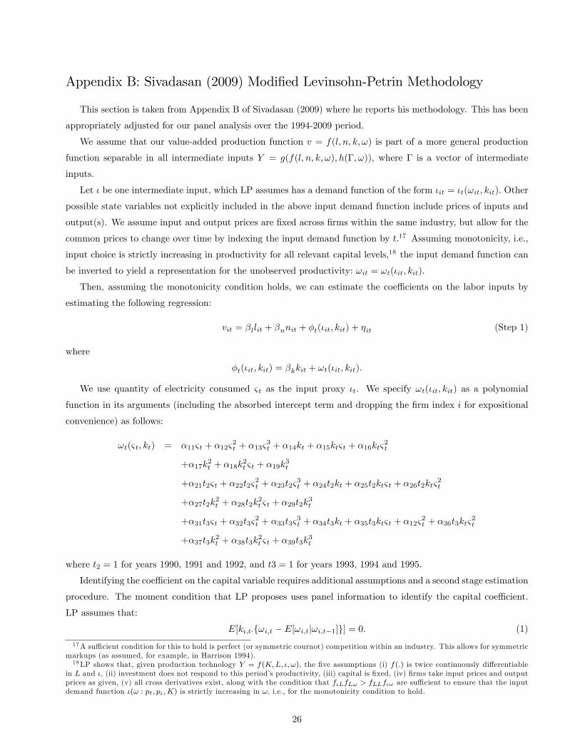
Appendix B: Sivadasan (2009) Modified Levinsohn-Petrin Methodology

This section is taken from Appendix B of Sivadasan (2009) where he reports his methodology. This has been

appropriately adjusted for our panel analysis over the 1994-2009 period.

We assume that our value-added production function v = f(l, n, k, ω) is part of a more general production

function separable in all intermediate inputs Y = g(f(l, n, k, ω), h(Γ, ω)), where Γ is a vector of intermediate

inputs.

Let ι be one intermediate input, which LP assumes has a demand function of the form ιit = ιt(ωit, kit). Other

possible state variables not explicitly included in the above input demand function include prices of inputs and

output(s). We assume input and output prices are fixed across firms within the same industry, but allow for the

common prices to change over time by indexing the input demand function by t.17 Assuming monotonicity, i.e.,

input choice is strictly increasing in productivity for all relevant capital levels,18 the input demand function can

be inverted to yield a representation for the unobserved productivity: ωit = ωt(ιit, kit).

Then, assuming the monotonicity condition holds, we can estimate the coeffi cients on the labor inputs by

estimating the following regression:

vit = βllit + βnnit + φt(ιit, kit) + ηit (Step 1)

where

φt(ιit, kit) = βkkit + ωt(ιit, kit).

We use quantity of electricity consumed ςt as the input proxy ιt. We specify ωt(ιit, kit) as a polynomial

function in its arguments (including the absorbed intercept term and dropping the firm index i for expositional

convenience) as follows:

ωt(ςt, kt) = α11ςt + α12ς2t + α13ς

3t + α14kt + α15ktςt + α16ktς

2t

+α17k2t + α18k

2t ςt + α19k

3t

+α21t2ςt + α22t2ς2t + α23t2ς

3t + α24t2kt + α25t2ktςt + α26t2ktς

2t

+α27t2k2t + α28t2k

2t ςt + α29t2k

3t

+α31t3ςt + α32t3ς2t + α33t3ς

3t + α34t3kt + α35t3ktςt + α12ς

2t + α36t3ktς

2t

+α37t3k2t + α38t3k

2t ςt + α39t3k

3t

where t2 = 1 for years 1990, 1991 and 1992, and t3 = 1 for years 1993, 1994 and 1995.

Identifying the coeffi cient on the capital variable requires additional assumptions and a second stage estimation

procedure. The moment condition that LP proposes uses panel information to identify the capital coeffi cient.

LP assumes that:

E[ki,t·{ωi,t − E[ωi,t|ωi,t−1]}] = 0. (1)

17A suffi cient condition for this to hold is perfect (or symmetric cournot) competition within an industry. This allows for symmetricmarkups (as assumed, for example, in Harrison 1994).18LP shows that, given production technology Y = f(K,L, ι, ω), the five assumptions (i) f(.) is twice continuously differentiable

in L and ι, (ii) investment does not respond to this period’s productivity, (iii) capital is fixed, (iv) firms take input prices and outputprices as given, (v) all cross derivatives exist, along with the condition that fιLfLω > fLLfιω are suffi cient to ensure that the inputdemand function ι(ω : pt, pι,K) is strictly increasing in ω, i.e., for the monotonicity condition to hold.

26

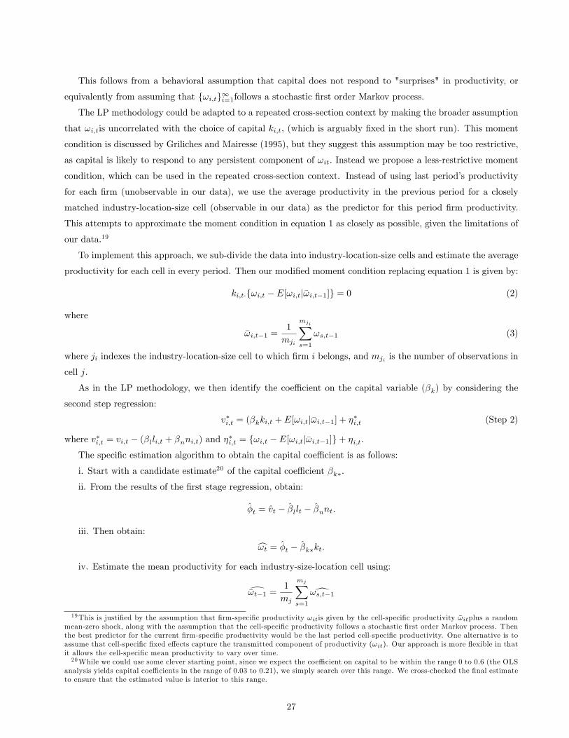
This follows from a behavioral assumption that capital does not respond to "surprises" in productivity, or

equivalently from assuming that {ωi,t}∞i=1follows a stochastic first order Markov process.The LP methodology could be adapted to a repeated cross-section context by making the broader assumption

that ωi,tis uncorrelated with the choice of capital ki,t, (which is arguably fixed in the short run). This moment

condition is discussed by Griliches and Mairesse (1995), but they suggest this assumption may be too restrictive,

as capital is likely to respond to any persistent component of ωit. Instead we propose a less-restrictive moment

condition, which can be used in the repeated cross-section context. Instead of using last period’s productivity

for each firm (unobservable in our data), we use the average productivity in the previous period for a closely

matched industry-location-size cell (observable in our data) as the predictor for this period firm productivity.

This attempts to approximate the moment condition in equation 1 as closely as possible, given the limitations of

our data.19

To implement this approach, we sub-divide the data into industry-location-size cells and estimate the average

productivity for each cell in every period. Then our modified moment condition replacing equation 1 is given by:

ki,t·{ωi,t − E[ωi,t|ωi,t−1]} = 0 (2)

where

ωi,t−1 =1

mji

mji∑s=1

ωs,t−1 (3)

where ji indexes the industry-location-size cell to which firm i belongs, and mji is the number of observations in

cell j.

As in the LP methodology, we then identify the coeffi cient on the capital variable (βk) by considering the

second step regression:

v∗i,t = (βkki,t + E[ωi,t|ωi,t−1] + η∗i,t (Step 2)

where v∗i,t = vi,t − (βlli,t + βnni,t) and η∗i,t = {ωi,t − E[ωi,t|ωi,t−1]}+ ηi,t.

The specific estimation algorithm to obtain the capital coeffi cient is as follows:

i. Start with a candidate estimate20 of the capital coeffi cient βk∗.

ii. From the results of the first stage regression, obtain:

φt = vt − βllt − βnnt.

iii. Then obtain:

ωt = φt − βk∗kt.

iv. Estimate the mean productivity for each industry-size-location cell using:

ωt−1 =1

mj

mj∑s=1

ωs,t−119This is justified by the assumption that firm-specific productivity ωitis given by the cell-specific productivity ωitplus a random

mean-zero shock, along with the assumption that the cell-specific productivity follows a stochastic first order Markov process. Thenthe best predictor for the current firm-specific productivity would be the last period cell-specific productivity. One alternative is toassume that cell-specific fixed effects capture the transmitted component of productivity (ωit). Our approach is more flexible in thatit allows the cell-specific mean productivity to vary over time.20While we could use some clever starting point, since we expect the coeffi cient on capital to be within the range 0 to 0.6 (the OLS

analysis yields capital coeffi cients in the range of 0.03 to 0.21), we simply search over this range. We cross-checked the final estimateto ensure that the estimated value is interior to this range.

27

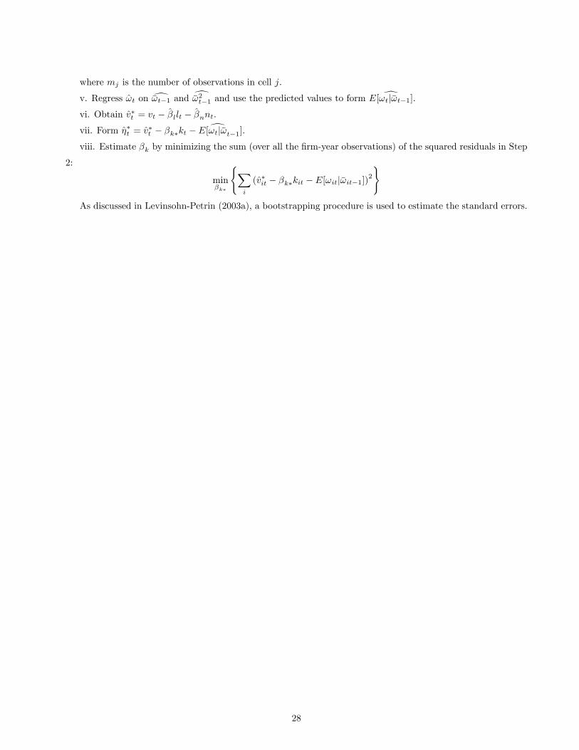
where mj is the number of observations in cell j.

v. Regress ωt on ωt−1 and ω2t−1 and use the predicted values to form E[ωt|ωt−1].vi. Obtain v∗t = vt − βllt − βnnt.vii. Form η∗t = v∗t − βk∗kt − E[ωt|ωt−1].viii. Estimate βk by minimizing the sum (over all the firm-year observations) of the squared residuals in Step

2:

minβk∗

{∑i

(v∗it − βk∗kit − E[ωit|ωit−1])2}

As discussed in Levinsohn-Petrin (2003a), a bootstrapping procedure is used to estimate the standard errors.

28

Figure 1: Highway networks in India

Figure 2: Straight-line IV framework routes

Figure 3a: Dynamics of log new output growth

Figure 3b: Dynamics of log total output growth

Figure 4a: Change in allocative efficiency, 2000→2009

Figure 4b: Using a 200 km band around GQ in 2000

Figure 4c: Considering the pre-period of 1994→2000

Figure 4d: Considering proximity to the NS-EW system

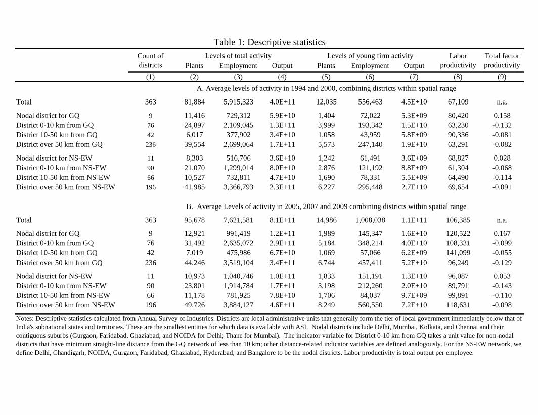
Plants Employment Output Plants Employment Output

(1) (2) (3) (4) (5) (6) (7) (8) (9)

Total 363 81,884 5,915,323 4.0E+11 12,035 556,463 4.5E+10 67,109 n.a.

Nodal district for GQ 9 11,416 729,312 5.9E+10 1,404 72,022 5.3E+09 80,420 0.158

District 0-10 km from GQ 76 24,897 2,109,045 1.3E+11 3,999 193,342 1.5E+10 63,230 -0.132

District 10-50 km from GQ 42 6,017 377,902 3.4E+10 1,058 43,959 5.8E+09 90,336 -0.081

District over 50 km from GQ 236 39,554 2,699,064 1.7E+11 5,573 247,140 1.9E+10 63,291 -0.082

Nodal district for NS-EW 11 8,303 516,706 3.6E+10 1,242 61,491 3.6E+09 68,827 0.028

District 0-10 km from NS-EW 90 21,070 1,299,014 8.0E+10 2,876 121,192 8.8E+09 61,304 -0.068

District 10-50 km from NS-EW 66 10,527 732,811 4.7E+10 1,690 78,331 5.5E+09 64,490 -0.114

District over 50 km from NS-EW 196 41,985 3,366,793 2.3E+11 6,227 295,448 2.7E+10 69,654 -0.091

Total 363 95,678 7,621,581 8.1E+11 14,986 1,008,038 1.1E+11 106,385 n.a.

Nodal district for GQ 9 12,921 991,419 1.2E+11 1,989 145,347 1.6E+10 120,522 0.167

District 0-10 km from GQ 76 31,492 2,635,072 2.9E+11 5,184 348,214 4.0E+10 108,331 -0.099

District 10-50 km from GQ 42 7,019 475,986 6.7E+10 1,069 57,066 6.2E+09 141,099 -0.055

District over 50 km from GQ 236 44,246 3,519,104 3.4E+11 6,744 457,411 5.2E+10 96,249 -0.129

Nodal district for NS-EW 11 10,973 1,040,746 1.0E+11 1,833 151,191 1.3E+10 96,087 0.053

District 0-10 km from NS-EW 90 23,801 1,914,784 1.7E+11 3,198 212,260 2.0E+10 89,791 -0.143

District 10-50 km from NS-EW 66 11,178 781,925 7.8E+10 1,706 84,037 9.7E+09 99,891 -0.110

District over 50 km from NS-EW 196 49,726 3,884,127 4.6E+11 8,249 560,550 7.2E+10 118,631 -0.098

Table 1: Descriptive statistics

Total factor

productivity

B. Average Levels of activity in 2005, 2007 and 2009 combining districts within spatial range

A. Average levels of activity in 1994 and 2000, combining districts within spatial range

Notes: Descriptive statistics calculated from Annual Survey of Industries. Districts are local administrative units that generally form the tier of local government immediately below that of

India's subnational states and territories. These are the smallest entities for which data is available with ASI. Nodal districts include Delhi, Mumbai, Kolkata, and Chennai and their

contiguous suburbs (Gurgaon, Faridabad, Ghaziabad, and NOIDA for Delhi; Thane for Mumbai). The indicator variable for District 0-10 km from GQ takes a unit value for non-nodal

districts that have minimum straight-line distance from the GQ network of less than 10 km; other distance-related indicator variables are defined analogously. For the NS-EW network, we

define Delhi, Chandigarh, NOIDA, Gurgaon, Faridabad, Ghaziabad, Hyderabad, and Bangalore to be the nodal districts. Labor productivity is total output per employee.

Levels of young firm activity Labor

productivity

Levels of total activityCount of

districts

Plants Employment Output Plants Employment Output

(1) (2) (3) (4) (5) (6)

Total 1.014 1.016 1.027 1.023 1.045 1.038

Nodal district for GQ 1.013 1.023 1.029 1.048 1.063 1.048

District 0-10 km from GQ 1.023 1.015 1.030 1.031 1.048 1.043

District 10-50 km from GQ 1.018 1.018 1.028 1.001 1.024 1.003

District over 50 km from GQ 1.011 1.018 1.026 1.022 1.050 1.043

Nodal district for NS-EW 1.031 1.053 1.043 1.055 1.082 1.057

District 0-10 km from NS-EW 1.012 1.028 1.031 1.013 1.048 1.035

District 10-50 km from NS-EW 1.006 1.005 1.020 1.001 1.006 1.025

District over 50 km from NS-EW 1.016 1.010 1.026 1.032 1.051 1.041

Ratio of 0-10 to 50+ GQ groups 1.012 0.997 1.003 1.009 0.999 1.000

Ratio of 0-10 to 50+ NS-EW groups 0.996 1.018 1.005 0.982 0.997 0.994

Ratio of 0-10 GQ to 0-10 NS-EW groups 1.011 0.988 0.999 1.018 1.000 1.007

Nodal district for GQ -0.004 0.007 0.000 0.016 0.015 0.018

District 0-10 km from GQ 0.025 -0.011 0.016 0.014 -0.002 0.022

District 10-50 km from GQ 0.000 -0.001 -0.003 -0.017 -0.022 -0.075

District over 50 km from GQ -0.021 0.005 -0.013 -0.013 0.010 0.035

Nodal district for NS-EW 0.013 0.049 0.034 0.019 0.039 0.030

District 0-10 km from NS-EW -0.009 0.032 0.011 -0.026 -0.007 -0.024

District 10-50 km from NS-EW -0.012 -0.021 -0.023 -0.027 -0.057 -0.037

District over 50 km from NS-EW 0.007 -0.060 -0.022 0.033 0.025 0.031

Table 1: Descriptive statistics, continued

C. Log growth in activity from 1994/2000 to 2005/2007/2009

D. Change in share of activity from 1994/2000 to 2005/2007/2009

Notes: See notes above. Share changes in Panel D are calculated separately for distances from the GQ and NS-EW networks such that they sum to zero for

each group.

Levels of total activity Levels of young firm activity

Plants Employment Output Plants Employment Output

(1) (2) (3) (4) (5) (6) (7) (8) (9) (10)

(0,1) Nodal district 1.467 1.255 1.413 1.640 2.004 2.468 0.138 1.971 0.382 0.393

(0.496) (0.464) (0.480) (0.499) (0.543) (0.621) (0.111) (0.195) (0.065) (0.069)0.000 0.000 0.000 0.000 0.000 0.000 0.000 0.000 0.000 0.000

(0,1) District 0-10 km from GQ 0.364 0.235 0.443 0.815 0.882 1.069 0.199 0.163 0.121 0.130

(0.128) (0.144) (0.163) (0.161) (0.198) (0.277) (0.074) (0.195) (0.055) (0.056)0.000 0.000 0.000 0.000 0.000 0.000 0.000 0.000 0.000 0.000

(0,1) District 10-50 km from GQ -0.199 -0.325 -0.175 -0.238 -0.087 -0.281 0.157 0.286 0.098 0.095

(0.185) (0.222) (0.293) (0.237) (0.314) (0.455) (0.126) (0.280) (0.091) (0.094)

(0,1) Nodal district 0.541 0.468 0.493 0.831 0.964 0.927 0.004 1.367 0.239 0.249

(0.591) (0.657) (0.677) (0.718) (0.858) (0.957) (0.151) (0.280) (0.096) (0.100)0.000 0.000 0.000 0.000 0.000 0.000 0.000 0.000 0.000 0.000

(0,1) District 0-10 km from GQ 0.312 0.233 0.427 0.616 0.555 0.680 0.241 0.112 0.169 0.185

(0.124) (0.129) (0.157) (0.174) (0.201) (0.286) (0.085) (0.215) (0.060) (0.062)0.000 0.000 0.000 0.000 0.000 0.000 0.000 0.000 0.000 0.000

(0,1) District 10-50 km from GQ -0.117 -0.202 -0.024 -0.115 -0.025 -0.194 0.177 0.403 0.151 0.155

(0.161) (0.196) (0.271) (0.207) (0.279) (0.416) (0.127) (0.288) (0.087) (0.090)

(0,1) Nodal district 0.773 0.671 0.661 1.110 1.087 1.033 -0.011 1.292 0.256 0.259

(0.643) (0.718) (0.728) (0.797) (0.963) (1.062) (0.157) (0.342) (0.114) (0.117)0.000 0.000 0.000 0.000 0.000 0.000 0.000 0.000 0.000 0.000

(0,1) District 0-10 km from GQ 0.334 0.194 0.370 0.503 0.361 0.490 0.189 0.235 0.160 0.177

(0.147) (0.172) (0.211) (0.208) (0.246) (0.345) (0.113) (0.262) (0.073) (0.075)0.000 0.000 0.000 0.000 0.000 0.000 0.000 0.000 0.000 0.000

(0,1) District 10-50 km from GQ -0.145 -0.275 -0.147 -0.190 -0.178 -0.382 0.113 0.424 0.123 0.126

(0.186) (0.237) (0.320) (0.224) (0.309) (0.463) (0.147) (0.324) (0.102) (0.106)

C. Panel B including state fixed effects

Notes: Long-differenced estimations consider changes in the location and productivity of organized-sector manufacturing activity in 311 Indian districts from 2000 to 2007-2009 from the

Annual Survey of Industries (ASI). Explanatory variables are indicators for distance from the GQ network that was upgraded starting in 2001. Estimations consider the effects relative to

districts more than 50 km from the GQ network. Column headers list dependent variables. Young plants are those less than four years old. Labor productivity is total output per employee

in district, and TFP is weighted average of Sivadasan (2009) approach to Olley-Pakes estimations of establishment-level productivity with repeated cross-section data. Outcome variables

are winsorized at their 1% and 99% levels, and entry variables are coded at the 1% level where no entry is observed to maintain a consistent sample. Estimations report standard errors,

have 311 observations, control for the level of district activity in 2000, and weight observations by log total district population in 2001. Initial district conditions include variables for

national highway access, state highway access, and broad-gauge railroad access and district-level measures from 2000 Census of log total population, age profile, female-male sex ratio,

population share in urban areas, population share in scheduled castes or tribes, literacy rates, and an index of within-district infrastructure. Appendix Table 1 reports the coefficients for

these controls for the estimation in Panel B.

A. Base spatial horizon measuring effects relative to districts 50+ km from the GQ network

DV: Change in manufacturing trait

listed in column header

B. Panel A including covariates for initial district conditions and additional road and railroad traits

Table 2: Long-differenced estimations of the impact of GQ improvements, comparing 2007-2009 to 2000

Log levels of total activity Log levels of young firm activity Log labor

productivity

Total factor

productivity

Log average

wage

Log cost per

employee

Plants Employment Output Plants Employment Output

(1) (2) (3) (4) (5) (6) (7) (8) (9) (10)

(0,1) Nodal district 0.539 0.470 0.487 0.833 0.975 0.928 -0.003 1.377 0.243 0.253

(0.594) (0.659) (0.681) (0.720) (0.860) (0.961) (0.153) (0.281) (0.096) (0.101)0 0 0 0 0 0 0 0 0 0

(0,1) District 0-10 km from GQ * 0.295 0.253 0.382 0.636 0.633 0.692 0.194 0.181 0.199 0.211

(0,1) New construction district (0.129) (0.156) (0.171) (0.203) (0.258) (0.332) (0.083) (0.197) (0.065) (0.066)0 0 0 0 0 0 0 0 0 0

(0,1) District 0-10 km from GQ * 0.328 0.215 0.468 0.598 0.484 0.669 0.285 0.046 0.140 0.160

(0,1) Road upgrade district (0.179) (0.175) (0.236) (0.227) (0.238) (0.368) (0.121) (0.311) (0.084) (0.085)0 0 0 0 0 0 0 0 0 0

(0,1) District 10-50 km from GQ -0.117 -0.203 -0.023 -0.115 -0.028 -0.195 0.178 0.401 0.151 0.154

(0.161) (0.196) (0.271) (0.208) (0.280) (0.417) (0.127) (0.289) (0.087) (0.090)

(0,1) Nodal district 0.450 0.425 0.549 0.718 0.847 0.853 0.102 1.433 0.334 0.353

(0.597) (0.662) (0.687) (0.733) (0.871) (0.978) (0.166) (0.307) (0.105) (0.110)0 0 0 0 0 0 0 0 0 0

(0,1) District 0-10 km from GQ 0.226 0.196 0.490 0.509 0.445 0.612 0.344 0.175 0.259 0.284

(0.145) (0.156) (0.190) (0.213) (0.236) (0.342) (0.113) (0.245) (0.075) (0.077)0 0 0 0 0 0 0 0 0 0

(0,1) District 10-50 km from GQ -0.208 -0.242 0.043 -0.227 -0.141 -0.265 0.283 0.470 0.247 0.260

(0.176) (0.212) (0.282) (0.235) (0.312) (0.465) (0.146) (0.319) (0.098) (0.101)0 0 0 0 0 0 0 0 0 0

(0,1) District 50-125 km from GQ -0.268 -0.165 -0.043 -0.301 -0.355 -0.292 0.143 0.151 0.233 0.252

(0.150) (0.173) (0.242) (0.221) (0.265) (0.391) (0.167) (0.322) (0.097) (0.099)0 0 0 0 0 0 0 0 0 0

(0,1) District 125-200 km from GQ -0.068 0.018 0.286 -0.115 -0.072 0.032 0.247 0.095 0.114 0.131

(0.159) (0.191) (0.219) (0.245) (0.331) (0.454) (0.143) (0.323) (0.091) (0.094)

Log cost per

employee

D. Panel B separating new construction vs. improvements of existing roads

E. Panel B with extended spatial horizon measuring effects relative to districts 200+ km from the GQ network

Notes: See notes above. Panel D splits local effects along the GQ network by whether the development is new highway construction or the improvement of existing highways. Panel E

includes extended spatial rings to measure effects relative to districts 200 km away from the GQ network.

DV: Change in manufacturing trait

listed in column header

Table 2: Long-differenced estimations, continued

Log levels of total activity Log levels of young firm activity Log labor

productivity

Total factor

productivity

Log average

wage

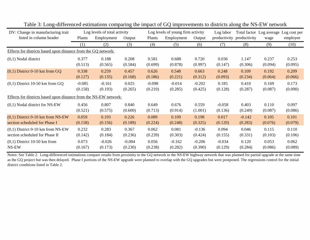
Plants Employment Output Plants Employment Output

(1) (2) (3) (4) (5) (6) (7) (8) (9) (10)

(0,1) Nodal district 0.377 0.188 0.208 0.581 0.688 0.720 0.036 1.147 0.237 0.253

(0.513) (0.565) (0.584) (0.699) (0.878) (0.997) (0.147) (0.306) (0.094) (0.095)0 0 0 0 0 0 0 0 0 0

(0,1) District 0-10 km from GQ 0.338 0.259 0.457 0.626 0.548 0.663 0.248 0.109 0.192 0.209

(0.127) (0.135) (0.168) (0.186) (0.221) (0.312) (0.093) (0.234) (0.064) (0.066)0 0 0 0 0 0 0 0 0 0

(0,1) District 10-50 km from GQ -0.085 -0.161 0.025 -0.098 -0.014 -0.202 0.185 0.410 0.169 0.173

(0.158) (0.193) (0.265) (0.210) (0.285) (0.425) (0.128) (0.287) (0.087) (0.090)

(0,1) Nodal district for NS-EW 0.456 0.807 0.840 0.649 0.676 0.559 -0.058 0.403 0.110 0.097

(0.521) (0.575) (0.600) (0.713) (0.914) (1.001) (0.136) (0.249) (0.087) (0.086)0 0 0 0 0 0 0 0 0 0

(0,1) District 0-10 km from NS-EW 0.059 0.193 0.226 0.089 0.109 0.198 0.017 -0.142 0.105 0.101

section scheduled for Phase I (0.158) (0.156) (0.189) (0.224) (0.248) (0.325) (0.120) (0.283) (0.076) (0.079)0 0 0 0 0 0 0 0 0 0

(0,1) District 0-10 km from NS-EW 0.232 0.283 0.367 0.062 0.081 -0.136 0.094 0.046 0.115 0.110

section scheduled for Phase II (0.142) (0.184) (0.236) (0.239) (0.303) (0.424) (0.155) (0.331) (0.103) (0.106)0 0 0 0 0 0 0 0 0 0

(0,1) District 10-50 km from 0.073 -0.026 -0.084 0.056 -0.162 -0.206 -0.034 0.120 0.053 0.062

NS-EW (0.167) (0.173) (0.230) (0.238) (0.282) (0.390) (0.129) (0.284) (0.086) (0.089)

Log cost per

employee

Notes: See Table 2. Long-differenced estimations compare results from proximity to the GQ network to the NS-EW highway network that was planned for partial upgrade at the same time

as the GQ project but was then delayed. Phase I portions of the NS-EW upgrade were planned to overlap with the GQ upgrades but were postponed. The regressions control for the initial

district conditions listed in Table 2.

Effects for districts based upon distance from the NS-EW network:

Effects for districts based upon distance from the GQ network:

DV: Change in manufacturing trait

listed in column header

Table 3: Long-differenced estimations comparing the impact of GQ improvements to districts along the NS-EW network

Log levels of total activity Log levels of young firm activity Log labor

productivity

Total factor

productivity

Log average

wage

Plants Employment Output Plants Employment Output

(1) (2) (3) (4) (5) (6) (7) (8) (9) (10)

(0,1) District 0-10 km from GQ 0.362 0.264 0.458 0.840 0.881 1.100 0.174 0.116 0.104 0.115

(0.122) (0.139) (0.158) (0.156) (0.191) (0.270) (0.070) (0.186) (0.053) (0.054)

0.168 -0.015 0.256 0.406 0.310 0.358 0.253 0.132 0.146 0.162

(0.122) (0.136) (0.168) (0.176) (0.218) (0.310) (0.085) (0.210) (0.061) (0.062)

0.195 0.056 0.315 0.450 0.418 0.448 0.220 0.319 0.175 0.186

(0.123) (0.139) (0.170) (0.179) (0.221) (0.312) (0.085) (0.199) (0.059) (0.060)

0.343 -0.030 0.513 0.818 0.622 0.713 0.490 0.256 0.282 0.313

(0.236) (0.280) (0.322) (0.323) (0.408) (0.585) (0.172) (0.405) (0.122) (0.125)

0.320 0.092 0.509 0.726 0.675 0.717 0.348 0.503 0.276 0.294

(0.193) (0.226) (0.266) (0.259) (0.330) (0.471) (0.136) (0.316) (0.098) (0.100)

Log average

wage

Log cost per

employee

(0,1) District 0-10 km from line

ROUTE 1

(0,1) District 0-10 km from line

ROUTE 2

(0,1) District 0-10 km from line

ROUTE 1

(0,1) District 0-10 km from line

ROUTE 2

Notes: See Table 2. Panel A modifies the base OLS estimation to exclude nodal districts and measure effects relative to districts 10+ km from the GQ network. This sample contains 302

districts. Panel B reports reduced-form estimations of whether or not a district edge is within 10 km of a straight line between nodal districts. Panel C reports IV estimations that

instrument being within 10 km from the GQ network with being within 10 km of the straight line between nodal districts. Route 1 does not connect Bangalore directly, with the first-stage

elasticity of 0.43 (0.05) and the associated F-statistic of 74.5. Route 2 treats Bangalore as a connection point, with the first-stage elasticity of 0.54 (0.05) and the associated F-statistic of

138.1.

B. Reduced-form estimates for distance from a straight-line between nodal districts

C. IV estimates using distance from a straight-line between nodal districts

A. Base OLS estimation that excludes nodal districts and measures effects relative to districts 10+ km from the GQ network

DV: Change in manufacturing trait

listed in column header

Table 4a: Instrumental variable estimations using distance from a straight line between nodal districts

Log levels of total activity Log levels of young firm activity Log labor

productivity

Total factor

productivity

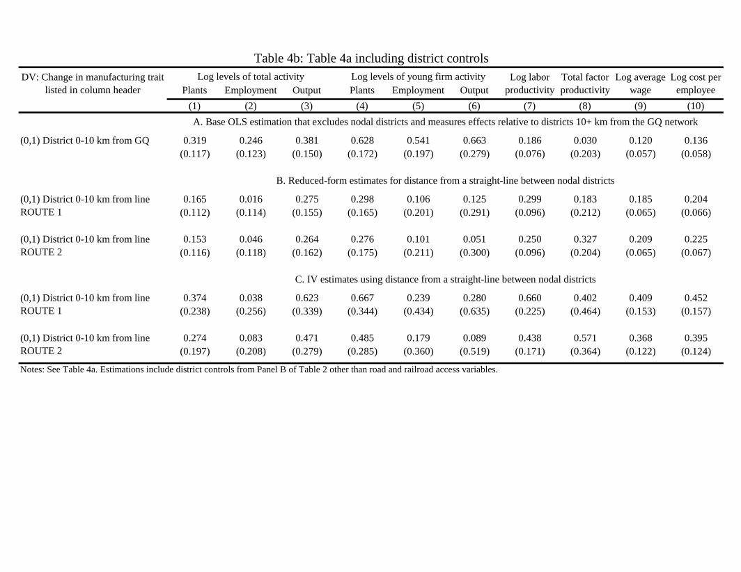
Plants Employment Output Plants Employment Output

(1) (2) (3) (4) (5) (6) (7) (8) (9) (10)

(0,1) District 0-10 km from GQ 0.319 0.246 0.381 0.628 0.541 0.663 0.186 0.030 0.120 0.136

(0.117) (0.123) (0.150) (0.172) (0.197) (0.279) (0.076) (0.203) (0.057) (0.058)

0.165 0.016 0.275 0.298 0.106 0.125 0.299 0.183 0.185 0.204

(0.112) (0.114) (0.155) (0.165) (0.201) (0.291) (0.096) (0.212) (0.065) (0.066)

0.153 0.046 0.264 0.276 0.101 0.051 0.250 0.327 0.209 0.225

(0.116) (0.118) (0.162) (0.175) (0.211) (0.300) (0.096) (0.204) (0.065) (0.067)

0.374 0.038 0.623 0.667 0.239 0.280 0.660 0.402 0.409 0.452

(0.238) (0.256) (0.339) (0.344) (0.434) (0.635) (0.225) (0.464) (0.153) (0.157)

0.274 0.083 0.471 0.485 0.179 0.089 0.438 0.571 0.368 0.395

(0.197) (0.208) (0.279) (0.285) (0.360) (0.519) (0.171) (0.364) (0.122) (0.124)

(0,1) District 0-10 km from line

ROUTE 2

Notes: See Table 4a. Estimations include district controls from Panel B of Table 2 other than road and railroad access variables.

A. Base OLS estimation that excludes nodal districts and measures effects relative to districts 10+ km from the GQ network

B. Reduced-form estimates for distance from a straight-line between nodal districts

(0,1) District 0-10 km from line

ROUTE 1

(0,1) District 0-10 km from line

ROUTE 2

C. IV estimates using distance from a straight-line between nodal districts

(0,1) District 0-10 km from line

ROUTE 1

Table 4b: Table 4a including district controls

DV: Change in manufacturing trait

listed in column header

Log levels of total activity Log levels of young firm activity Log labor

productivity

Total factor

productivity

Log average

wage

Log cost per

employee

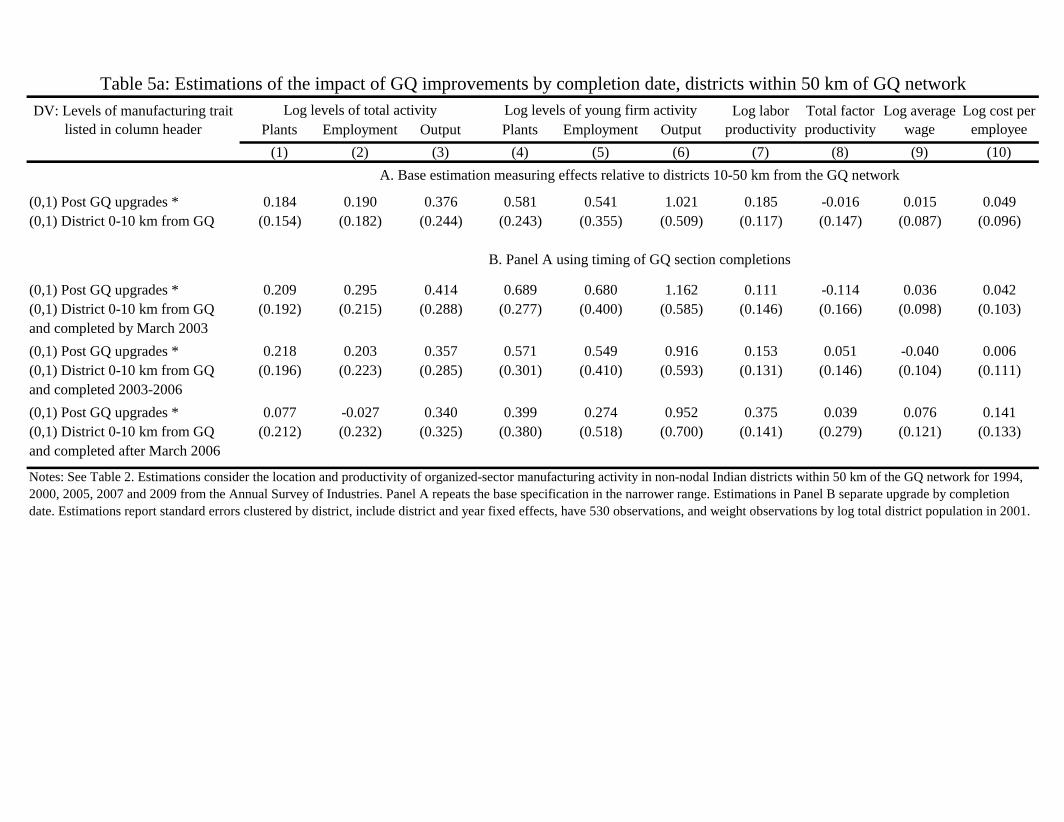
Plants Employment Output Plants Employment Output

(1) (2) (3) (4) (5) (6) (7) (8) (9) (10)

(0,1) Post GQ upgrades * 0.184 0.190 0.376 0.581 0.541 1.021 0.185 -0.016 0.015 0.049

(0,1) District 0-10 km from GQ (0.154) (0.182) (0.244) (0.243) (0.355) (0.509) (0.117) (0.147) (0.087) (0.096)

0 0 0 0 0 0 0

(0,1) Post GQ upgrades * 0.209 0.295 0.414 0.689 0.680 1.162 0.111 -0.114 0.036 0.042

(0,1) District 0-10 km from GQ (0.192) (0.215) (0.288) (0.277) (0.400) (0.585) (0.146) (0.166) (0.098) (0.103)

and completed by March 2003

(0,1) Post GQ upgrades * 0.218 0.203 0.357 0.571 0.549 0.916 0.153 0.051 -0.040 0.006

(0,1) District 0-10 km from GQ (0.196) (0.223) (0.285) (0.301) (0.410) (0.593) (0.131) (0.146) (0.104) (0.111)

and completed 2003-2006

(0,1) Post GQ upgrades * 0.077 -0.027 0.340 0.399 0.274 0.952 0.375 0.039 0.076 0.141

(0,1) District 0-10 km from GQ (0.212) (0.232) (0.325) (0.380) (0.518) (0.700) (0.141) (0.279) (0.121) (0.133)

Log cost per

employee

A. Base estimation measuring effects relative to districts 10-50 km from the GQ network

Notes: See Table 2. Estimations consider the location and productivity of organized-sector manufacturing activity in non-nodal Indian districts within 50 km of the GQ network for 1994,

2000, 2005, 2007 and 2009 from the Annual Survey of Industries. Panel A repeats the base specification in the narrower range. Estimations in Panel B separate upgrade by completion

date. Estimations report standard errors clustered by district, include district and year fixed effects, have 530 observations, and weight observations by log total district population in 2001.

DV: Levels of manufacturing trait

listed in column header

and completed after March 2006

Table 5a: Estimations of the impact of GQ improvements by completion date, districts within 50 km of GQ network

Log levels of total activity Log levels of young firm activity Log labor

productivity

Total factor

productivity

B. Panel A using timing of GQ section completions

Log average

wage

Plants Employment Output Plants Employment Output

(1) (2) (3) (4) (5) (6) (7) (8) (9) (10)

(0,1) Year 1999 * 0.035 0.188 0.359 -0.140 0.093 0.271 0.170 -0.389 0.128 0.166

(0,1) District 0-10 km from GQ (0.184) (0.255) (0.440) (0.265) (0.376) (0.625) (0.223) (0.309) (0.154) (0.168)

(0,1) Year 2000 * 0.052 0.034 0.044 -0.048 0.216 0.359 0.016 -0.032 -0.075 -0.029

(0,1) District 0-10 km from GQ (0.187) (0.168) (0.225) (0.280) (0.370) (0.646) (0.146) (0.264) (0.105) (0.113)

(0,1) Year 2001 * -0.152 -0.147 -0.276 -0.108 0.086 0.172 -0.128 -0.090 -0.112 -0.072

(0,1) District 0-10 km from GQ (0.210) (0.195) (0.249) (0.394) (0.454) (0.730) (0.176) (0.287) (0.105) (0.109)

(0,1) Year 2002 * 0.036 0.105 0.172 0.165 0.553 1.055 0.092 -0.080 0.037 0.088

(0,1) District 0-10 km from GQ (0.202) (0.201) (0.268) (0.334) (0.357) (0.539) (0.138) (0.240) (0.097) (0.119)

(0,1) Year 2003 * 0.036 0.094 0.077 0.188 0.561 0.992 -0.019 -0.168 -0.081 -0.037

(0,1) District 0-10 km from GQ (0.211) (0.240) (0.297) (0.331) (0.384) (0.534) (0.122) (0.273) (0.109) (0.124)

(0,1) Year 2004 * 0.175 0.134 0.303 0.658 1.093 1.785 0.168 -0.350 -0.020 0.034

(0,1) District 0-10 km from GQ (0.139) (0.157) (0.276) (0.306) (0.365) (0.499) (0.190) (0.260) (0.111) (0.123)

(0,1) Year 2005 * 0.063 0.058 0.199 0.431 0.789 1.363 0.142 -0.448 -0.059 -0.002

(0,1) District 0-10 km from GQ (0.142) (0.147) (0.198) (0.306) (0.417) (0.543) (0.117) (0.278) (0.089) (0.102)

(0,1) Year 2006 * 0.023 0.024 0.099 0.444 0.668 0.927 0.077 0.098 -0.068 -0.065

(0,1) District 0-10 km from GQ (0.150) (0.129) (0.173) (0.297) (0.383) (0.479) (0.117) (0.258) (0.083) (0.084)

(0,1) Year 2007 * 0.127 0.026 0.134 0.416 0.530 1.072 0.108 -0.076 -0.030 0.027

(0,1) District 0-10 km from GQ (0.142) (0.136) (0.172) (0.283) (0.427) (0.547) (0.125) (0.220) (0.089) (0.101)

(0,1) Year 2008 * 0.102 0.148 0.352 0.375 0.559 1.135 0.205 0.092 -0.019 0.015

(0,1) District 0-10 km from GQ (0.156) (0.158) (0.194) (0.282) (0.346) (0.475) (0.134) (0.235) (0.097) (0.108)

(0,1) Year 2009 * 0.338 0.399 0.553 0.905 0.730 1.079 0.156 -0.297 -0.095 -0.057

(0,1) District 0-10 km from GQ (0.199) (0.263) (0.359) (0.290) (0.352) (0.480) (0.169) (0.306) (0.115) (0.125)

Notes: See Table 2. Dynamic estimations consider the location and productivity of organized-sector manufacturing activity in non-nodal Indian districts within 50 km of the GQ network

for 1994-2009 from the Annual Survey of Industries. The interaction terms quantify the differential effect for GQ upgrades for non-nodal districts within 10 km of the GQ network

compared to districts that are 10-50 km from the GQ network by year, with 1994 as the reference year. The GQ upgrades commenced in 2001. Estimations report standard errors

clustered by district, include district and year fixed effects, have 1188 observations, and weight observations by log total district population in 2001.

Table 5b: Estimations of the impact of GQ improvements by year, districts within 50 km of GQ network

DV: Levels of manufacturing trait

listed in column header

Log levels of total activity Log levels of young firm activity Log labor

productivity

Total factor

productivity

Log average

wage

Log cost per

employee

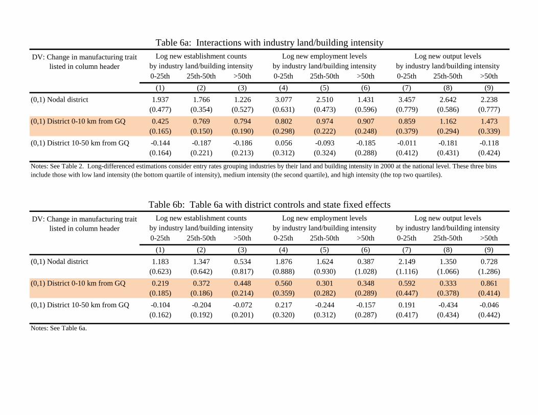
0-25th 25th-50th >50th 0-25th 25th-50th >50th 0-25th 25th-50th >50th

(1) (2) (3) (4) (5) (6) (7) (8) (9)

(0,1) Nodal district 1.937 1.766 1.226 3.077 2.510 1.431 3.457 2.642 2.238

(0.477) (0.354) (0.527) (0.631) (0.473) (0.596) (0.779) (0.586) (0.777)0 0 0 0 0 0 0 0 0

(0,1) District 0-10 km from GQ 0.425 0.769 0.794 0.802 0.974 0.907 0.859 1.162 1.473

(0.165) (0.150) (0.190) (0.298) (0.222) (0.248) (0.379) (0.294) (0.339)0 0 0 0 0 0 0 0 0

(0,1) District 10-50 km from GQ -0.144 -0.187 -0.186 0.056 -0.093 -0.185 -0.011 -0.181 -0.118

(0.164) (0.221) (0.213) (0.312) (0.324) (0.288) (0.412) (0.431) (0.424)

0-25th 25th-50th >50th 0-25th 25th-50th >50th 0-25th 25th-50th >50th

(1) (2) (3) (4) (5) (6) (7) (8) (9)

(0,1) Nodal district 1.183 1.347 0.534 1.876 1.624 0.387 2.149 1.350 0.728

(0.623) (0.642) (0.817) (0.888) (0.930) (1.028) (1.116) (1.066) (1.286)0 0 0 0 0 0 0 0 0

(0,1) District 0-10 km from GQ 0.219 0.372 0.448 0.560 0.301 0.348 0.592 0.333 0.861

(0.185) (0.186) (0.214) (0.359) (0.282) (0.289) (0.447) (0.378) (0.414)0 0 0 0 0 0 0 0 0

(0,1) District 10-50 km from GQ -0.104 -0.204 -0.072 0.217 -0.244 -0.157 0.191 -0.434 -0.046

(0.162) (0.192) (0.201) (0.320) (0.312) (0.287) (0.417) (0.434) (0.442)

Notes: See Table 6a.

DV: Change in manufacturing trait

listed in column header

Table 6b: Table 6a with district controls and state fixed effects

Log new establishment counts Log new employment levels Log new output levels

by industry land/building intensity by industry land/building intensity by industry land/building intensity

Notes: See Table 2. Long-differenced estimations consider entry rates grouping industries by their land and building intensity in 2000 at the national level. These three bins

include those with low land intensity (the bottom quartile of intensity), medium intensity (the second quartile), and high intensity (the top two quartiles).

DV: Change in manufacturing trait

listed in column header

Table 6a: Interactions with industry land/building intensity

Log new establishment counts Log new employment levels Log new output levels

by industry land/building intensity by industry land/building intensity by industry land/building intensity

Plants Employment Output Plants Employment Output

(1) (2) (3) (4) (5) (6) (7) (8) (9) (10)

(0,1) District 0-10 km from GQ 0.490 0.501 0.583 1.017 0.932 1.343 0.020 -0.129 0.016 0.030

(0.205) (0.234) (0.284) (0.265) (0.327) (0.480) (0.126) (0.281) (0.093) (0.096)

(0,1) District 0-10 km from GQ 0.756 0.807 0.825 1.269 1.311 1.784 0.010 0.115 0.084 0.102

Above median (0.243) (0.275) (0.286) (0.312) (0.349) (0.492) (0.130) (0.294) (0.098) (0.100)

(0,1) District 0-10 km from GQ 0.323 0.315 0.405 0.832 0.663 0.992 0.030 -0.383 -0.055 -0.044

Median value and below (0.229) (0.268) (0.359) (0.294) (0.373) (0.557) (0.141) (0.328) (0.104) (0.107)

(0,1) District 0-10 km from GQ 0.514 0.776 0.848 1.092 1.273 1.875 0.060 0.173 0.115 0.134

Above median (0.232) (0.264) (0.299) (0.299) (0.334) (0.485) (0.127) (0.286) (0.098) (0.100)

(0,1) District 0-10 km from GQ 0.469 0.273 0.331 0.940 0.602 0.783 -0.032 -0.522 -0.116 -0.108

Median value and below (0.236) (0.269) (0.354) (0.289) (0.386) (0.564) (0.147) (0.344) (0.104) (0.109)

(0,1) District 0-10 km from GQ 0.503 0.591 0.566 1.048 1.154 1.481 -0.044 0.095 0.043 0.055

Above median (0.238) (0.239) (0.266) (0.336) (0.375) (0.522) (0.123) (0.284) (0.097) (0.098)

(0,1) District 0-10 km from GQ 0.482 0.444 0.595 0.995 0.776 1.234 0.086 -0.357 -0.011 0.004

Median value and below (0.228) (0.274) (0.353) (0.267) (0.362) (0.540) (0.146) (0.341) (0.103) (0.108)

(0,1) District 0-10 km from GQ 0.474 0.281 0.546 1.039 0.769 1.095 0.059 -0.222 -0.002 0.010

Above median (0.228) (0.251) (0.323) (0.310) (0.390) (0.596) (0.151) (0.347) (0.112) (0.117)

(0,1) District 0-10 km from GQ 0.499 0.623 0.604 1.006 1.023 1.478 0.004 -0.087 0.024 0.039

Median value and below (0.226) (0.258) (0.312) (0.286) (0.349) (0.504) (0.127) (0.299) (0.098) (0.100)

Table 7: Interactions with district traits

DV: Change in manufacturing trait

listed in column header

Log levels of total activity Log levels of young firm activity Log labor

productivity

Total factor

productivity

Log average

wage

Log cost per

employee

A. Base OLS estimation that excludes nodal districts and measures effects relative to districts 10-50 km from the GQ network

B. Panel A with interaction split using median of district population density

C. Panel A with interaction split using median of district literacy

D. Panel A with interaction split using median of district infrastructure index

E. Panel A with interaction split using median of district distance from nodal city

Notes: See Table 2.

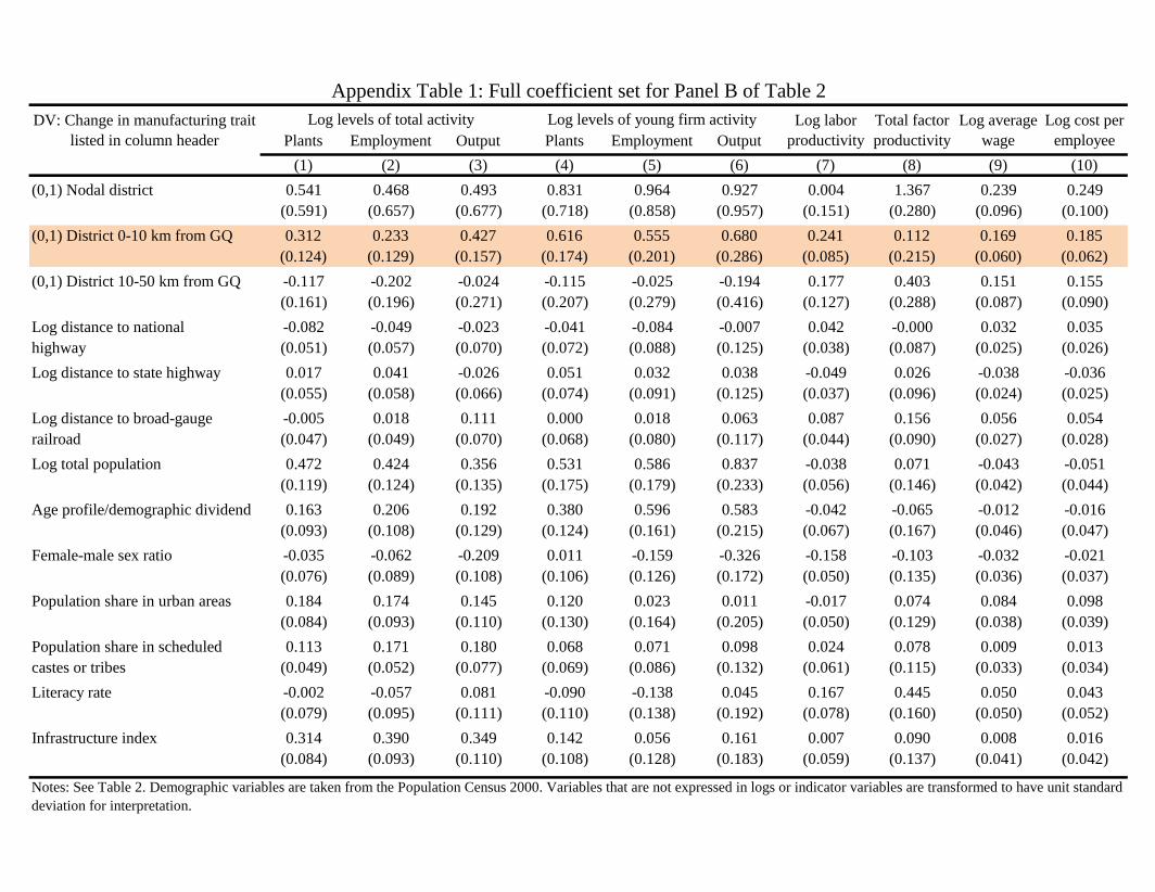
Plants Employment Output Plants Employment Output

(1) (2) (3) (4) (5) (6) (7) (8) (9) (10)

(0,1) Nodal district 0.541 0.468 0.493 0.831 0.964 0.927 0.004 1.367 0.239 0.249

(0.591) (0.657) (0.677) (0.718) (0.858) (0.957) (0.151) (0.280) (0.096) (0.100)0.000 0.000 0.000 0.000 0.000 0.000 0.000 0.000 0.000 0.000

(0,1) District 0-10 km from GQ 0.312 0.233 0.427 0.616 0.555 0.680 0.241 0.112 0.169 0.185

(0.124) (0.129) (0.157) (0.174) (0.201) (0.286) (0.085) (0.215) (0.060) (0.062)0.000 0.000 0.000 0.000 0.000 0.000 0.000 0.000 0.000 0.000

(0,1) District 10-50 km from GQ -0.117 -0.202 -0.024 -0.115 -0.025 -0.194 0.177 0.403 0.151 0.155

(0.161) (0.196) (0.271) (0.207) (0.279) (0.416) (0.127) (0.288) (0.087) (0.090)0.000 0.000 0.000 0.000 0.000 0.000 0.000 0.000 0.000 0.000

Log distance to national -0.082 -0.049 -0.023 -0.041 -0.084 -0.007 0.042 -0.000 0.032 0.035

highway (0.051) (0.057) (0.070) (0.072) (0.088) (0.125) (0.038) (0.087) (0.025) (0.026)0.000 0.000 0.000 0.000 0.000 0.000 0.000 0.000 0.000 0.000

Log distance to state highway 0.017 0.041 -0.026 0.051 0.032 0.038 -0.049 0.026 -0.038 -0.036

(0.055) (0.058) (0.066) (0.074) (0.091) (0.125) (0.037) (0.096) (0.024) (0.025)0.000 0.000 0.000 0.000 0.000 0.000 0.000 0.000 0.000 0.000

Log distance to broad-gauge -0.005 0.018 0.111 0.000 0.018 0.063 0.087 0.156 0.056 0.054

railroad (0.047) (0.049) (0.070) (0.068) (0.080) (0.117) (0.044) (0.090) (0.027) (0.028)0.000 0.000 0.000 0.000 0.000 0.000 0.000 0.000 0.000 0.000

Log total population 0.472 0.424 0.356 0.531 0.586 0.837 -0.038 0.071 -0.043 -0.051

(0.119) (0.124) (0.135) (0.175) (0.179) (0.233) (0.056) (0.146) (0.042) (0.044)0.000 0.000 0.000 0.000 0.000 0.000 0.000 0.000 0.000 0.000

Age profile/demographic dividend 0.163 0.206 0.192 0.380 0.596 0.583 -0.042 -0.065 -0.012 -0.016

(0.093) (0.108) (0.129) (0.124) (0.161) (0.215) (0.067) (0.167) (0.046) (0.047)0.000 0.000 0.000 0.000 0.000 0.000 0.000 0.000 0.000 0.000

Female-male sex ratio -0.035 -0.062 -0.209 0.011 -0.159 -0.326 -0.158 -0.103 -0.032 -0.021

(0.076) (0.089) (0.108) (0.106) (0.126) (0.172) (0.050) (0.135) (0.036) (0.037)0.000 0.000 0.000 0.000 0.000 0.000 0.000 0.000 0.000 0.000

Population share in urban areas 0.184 0.174 0.145 0.120 0.023 0.011 -0.017 0.074 0.084 0.098

(0.084) (0.093) (0.110) (0.130) (0.164) (0.205) (0.050) (0.129) (0.038) (0.039)0.000 0.000 0.000 0.000 0.000 0.000 0.000 0.000 0.000 0.000

Population share in scheduled 0.113 0.171 0.180 0.068 0.071 0.098 0.024 0.078 0.009 0.013

castes or tribes (0.049) (0.052) (0.077) (0.069) (0.086) (0.132) (0.061) (0.115) (0.033) (0.034)0.000 0.000 0.000 0.000 0.000 0.000 0.000 0.000 0.000 0.000

Literacy rate -0.002 -0.057 0.081 -0.090 -0.138 0.045 0.167 0.445 0.050 0.043

(0.079) (0.095) (0.111) (0.110) (0.138) (0.192) (0.078) (0.160) (0.050) (0.052)0.000 0.000 0.000 0.000 0.000 0.000 0.000 0.000 0.000 0.000

Infrastructure index 0.314 0.390 0.349 0.142 0.056 0.161 0.007 0.090 0.008 0.016

(0.084) (0.093) (0.110) (0.108) (0.128) (0.183) (0.059) (0.137) (0.041) (0.042)

Notes: See Table 2. Demographic variables are taken from the Population Census 2000. Variables that are not expressed in logs or indicator variables are transformed to have unit standard

deviation for interpretation.

Appendix Table 1: Full coefficient set for Panel B of Table 2

DV: Change in manufacturing trait

listed in column header

Log levels of total activity Log levels of young firm activity Log labor

productivity

Total factor

productivity

Log average

wage

Log cost per

employee

Plants Employment Output Plants Employment Output

(1) (2) (3) (4) (5) (6) (7) (8) (9) (10)

(0,1) Nodal district 0.556 0.500 0.525 0.844 1.016 0.995 0.005 1.376 0.239 0.250

(0.593) (0.661) (0.679) (0.718) (0.861) (0.960) (0.154) (0.279) (0.097) (0.101)0 0 0 0 0 0 0 0 0 0

(0,1) District 0-10 km from GQ 0.304 0.227 0.425 0.609 0.553 0.679 0.244 0.108 0.167 0.184

(0.124) (0.130) (0.158) (0.175) (0.202) (0.289) (0.085) (0.216) (0.061) (0.062)0 0 0 0 0 0 0 0 0 0

(0,1) District 10-50 km from GQ -0.121 -0.197 -0.019 -0.128 -0.027 -0.193 0.176 0.401 0.152 0.156

(0.161) (0.197) (0.271) (0.205) (0.278) (0.417) (0.126) (0.289) (0.086) (0.090)

(0,1) Nodal district 0.559 0.498 0.496 0.847 0.968 0.955 -0.023 1.306 0.214 0.224

(0.592) (0.659) (0.675) (0.717) (0.856) (0.957) (0.150) (0.275) (0.095) (0.099)0 0 0 0 0 0 0 0 0 0

(0,1) District 0-10 km from GQ 0.334 0.271 0.432 0.638 0.560 0.717 0.208 0.037 0.139 0.156

(0.119) (0.127) (0.152) (0.167) (0.196) (0.277) (0.078) (0.202) (0.057) (0.058)

(0,1) Nodal district 0.552 0.503 0.506 0.825 0.960 0.936 -0.015 1.338 0.225 0.235

(0.582) (0.668) (0.674) (0.698) (0.841) (0.947) (0.151) (0.271) (0.094) (0.098)0 0 0 0 0 0 0 0 0 0

(0,1) District 0-10 km from GQ 0.335 0.256 0.450 0.640 0.582 0.711 0.240 0.113 0.168 0.185

(0.128) (0.133) (0.159) (0.176) (0.204) (0.288) (0.085) (0.215) (0.060) (0.062)0 0 0 0 0 0 0 0 0 0

(0,1) District 10-30 km from GQ 0.069 -0.148 0.008 0.226 0.215 0.138 0.125 0.170 0.089 0.091

(0.291) (0.372) (0.454) (0.327) (0.403) (0.550) (0.159) (0.280) (0.110) (0.113)0 0 0 0 0 0 0 0 0 0

(0,1) District 30-50 km from GQ -0.056 -0.017 0.185 -0.198 0.026 -0.205 0.221 0.648 0.209 0.217

(0.210) (0.192) (0.316) (0.278) (0.407) (0.615) (0.172) (0.435) (0.120) (0.125)

Log distance from GQ -0.110 -0.245 -0.305 -0.107 -0.178 -0.376 -0.069 -0.087 -0.037 -0.052

(0.164) (0.193) (0.280) (0.234) (0.266) (0.371) (0.117) (0.242) (0.081) (0.084)

Appendix Table 2: Further robustness checks on Panel A of Table 2

Log levels of total activity Log levels of young firm activity Log labor

productivity

Total factor

productivity

Log average

wage

Log cost per

employee

A. Excluding sample weights and including outlier districts

D. Using linear distance up to 50 kilometers in non-nodal districts within 50 km of GQ network

Notes: See Table 2.

C. Using a finer distance bins within 10-50 km range

DV: Change in manufacturing trait

listed in column header

B. Using just the first distance band

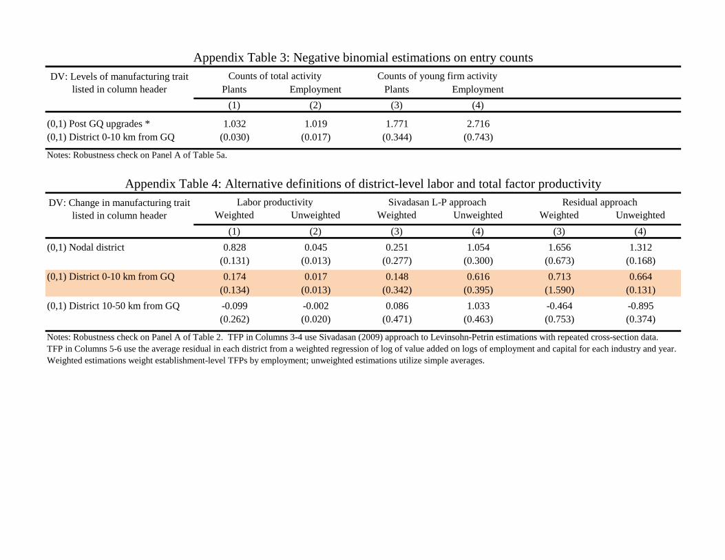
Plants Employment Plants Employment

(1) (2) (3) (4)0 0 0 0

(0,1) Post GQ upgrades * 1.032 1.019 1.771 2.716

(0,1) District 0-10 km from GQ (0.030) (0.017) (0.344) (0.743)

Weighted Unweighted Weighted Unweighted Weighted Unweighted

(1) (2) (3) (4) (3) (4)

(0,1) Nodal district 0.828 0.045 0.251 1.054 1.656 1.312

(0.131) (0.013) (0.277) (0.300) (0.673) (0.168)0 0 0 0 0 0

(0,1) District 0-10 km from GQ 0.174 0.017 0.148 0.616 0.713 0.664

(0.134) (0.013) (0.342) (0.395) (1.590) (0.131)0 0 0 0 0 0

(0,1) District 10-50 km from GQ -0.099 -0.002 0.086 1.033 -0.464 -0.895

(0.262) (0.020) (0.471) (0.463) (0.753) (0.374)

Notes: Robustness check on Panel A of Table 2. TFP in Columns 3-4 use Sivadasan (2009) approach to Levinsohn-Petrin estimations with repeated cross-section data.

TFP in Columns 5-6 use the average residual in each district from a weighted regression of log of value added on logs of employment and capital for each industry and year.

Weighted estimations weight establishment-level TFPs by employment; unweighted estimations utilize simple averages.

Appendix Table 3: Negative binomial estimations on entry counts

Counts of total activity

Notes: Robustness check on Panel A of Table 5a.

Appendix Table 4: Alternative definitions of district-level labor and total factor productivity

Labor productivity Residual approach

Counts of young firm activity

Sivadasan L-P approach

DV: Levels of manufacturing trait

listed in column header

DV: Change in manufacturing trait

listed in column header

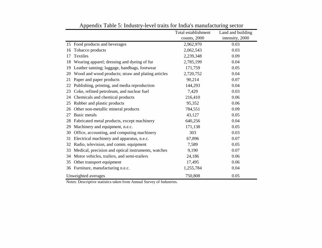
Total establishment Land and building

counts, 2000 intensity, 2000

15 Food products and beverages 2,962,970 0.03

16 Tobacco products 2,062,543 0.03

17 Textiles 2,239,348 0.09

18 Wearing apparel; dressing and dyeing of fur 2,785,199 0.04

19 Leather tanning; luggage, handbags, footwear 171,759 0.05

20 Wood and wood products; straw and plating articles 2,720,752 0.04

21 Paper and paper products 90,214 0.07

22 Publishing, printing, and media reproduction 144,293 0.04

23 Coke, refined petroleum, and nuclear fuel 7,429 0.03

24 Chemicals and chemical products 216,410 0.06

25 Rubber and plastic products 95,352 0.06

26 Other non-metallic mineral products 784,551 0.09

27 Basic metals 43,127 0.05

28 Fabricated metal products, except machinery 640,256 0.04

29 Machinery and equipment, n.e.c. 171,138 0.05

30 Office, accounting, and computing machinery 303 0.03

31 Electrical machinery and apparatus, n.e.c. 67,896 0.07

32 Radio, television, and comm. equipment 7,589 0.05

33 Medical, precision and optical instruments, watches 9,190 0.07

34 Motor vehicles, trailers, and semi-trailers 24,186 0.06

35 Other transport equipment 17,495 0.06

36 Furniture, manufacturing n.e.c. 1,255,784 0.04

Unweighted averages 750,808 0.05

Appendix Table 5: Industry-level traits for India's manufacturing sector

Notes: Descriptive statistics taken from Annual Survey of Industries.

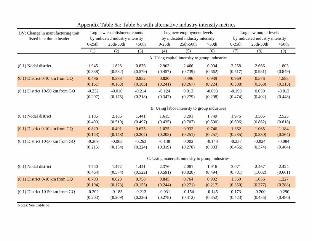
0-25th 25th-50th >50th 0-25th 25th-50th >50th 0-25th 25th-50th >50th

(1) (2) (3) (4) (5) (6) (7) (8) (9)

(0,1) Nodal district 1.945 1.828 0.876 2.903 2.466 0.994 3.258 2.666 1.803

(0.338) (0.532) (0.579) (0.457) (0.739) (0.662) (0.517) (0.981) (0.849)0 0 0 0 0 0 0 0 0

(0,1) District 0-10 km from GQ 0.496 0.383 0.852 0.820 0.496 0.939 0.969 0.576 1.585

(0.161) (0.163) (0.183) (0.241) (0.267) (0.224) (0.308) (0.368) (0.315)0 0 0 0 0 0 0 0 0

(0,1) District 10-50 km from GQ -0.232 -0.010 -0.214 -0.124 0.013 -0.093 -0.193 0.039 -0.013

(0.207) (0.175) (0.218) (0.347) (0.279) (0.298) (0.474) (0.402) (0.448)

(0,1) Nodal district 1.185 2.186 1.441 1.615 3.291 1.749 1.976 3.505 2.525

(0.490) (0.510) (0.497) (0.435) (0.707) (0.590) (0.696) (0.862) (0.818)0 0 0 0 0 0 0 0 0

(0,1) District 0-10 km from GQ 0.820 0.491 0.675 1.025 0.932 0.746 1.362 1.065 1.184

(0.143) (0.148) (0.204) (0.205) (0.251) (0.257) (0.285) (0.330) (0.364)0 0 0 0 0 0 0 0 0

(0,1) District 10-50 km from GQ -0.269 -0.063 -0.263 -0.138 0.002 -0.148 -0.237 -0.024 -0.084

(0.215) (0.154) (0.224) (0.319) (0.278) (0.303) (0.456) (0.374) (0.464)

(0,1) Nodal district 1.740 1.472 1.441 2.376 2.081 1.916 3.071 2.467 2.424

(0.464) (0.574) (0.522) (0.591) (0.820) (0.494) (0.781) (1.002) (0.661)0 0 0 0 0 0 0 0 0

(0,1) District 0-10 km from GQ 0.703 0.623 0.758 0.845 0.764 0.992 1.369 1.056 1.227

(0.194) (0.173) (0.155) (0.244) (0.271) (0.217) (0.350) (0.377) (0.288)0 0 0 0 0 0 0 0 0

(0,1) District 10-50 km from GQ -0.202 -0.183 -0.213 -0.031 -0.154 -0.145 0.173 -0.200 -0.290

(0.203) (0.209) (0.226) (0.278) (0.312) (0.352) (0.423) (0.435) (0.480)

by indicated industry intensity by indicated industry intensity

C. Using materials intensity to group industries

A. Using capital intensity to group industries

B. Using labor intensity to group industries

DV: Change in manufacturing trait

listed in column header

Notes: See Table 6a.

Appendix Table 6a: Table 6a with alternative industry intensity metrics

Log new establishment counts Log new employment levels Log new output levels

by indicated industry intensity

0-25th 25th-50th >50th 0-25th 25th-50th >50th 0-25th 25th-50th >50th

(1) (2) (3) (4) (5) (6) (7) (8) (9)

(0,1) Nodal district 1.414 1.119 0.391 1.693 1.416 0.309 1.214 1.400 0.793

(0.603) (0.706) (0.879) (0.875) (1.034) (1.105) (1.001) (1.397) (1.373)0 0 0 0 0 0 0 0 0

(0,1) District 0-10 km from GQ 0.159 0.272 0.494 0.361 0.318 0.352 0.336 0.318 1.013

(0.180) (0.174) (0.214) (0.290) (0.296) (0.274) (0.370) (0.412) (0.399)0 0 0 0 0 0 0 0 0

(0,1) District 10-50 km from GQ -0.285 0.057 -0.091 -0.255 0.100 -0.020 -0.496 0.079 0.195

(0.196) (0.172) (0.202) (0.348) (0.283) (0.284) (0.467) (0.404) (0.454)

(0,1) Nodal district 0.611 1.638 0.733 0.662 2.554 0.563 0.642 2.624 0.750

(0.715) (0.702) (0.763) (0.819) (1.054) (1.042) (1.153) (1.196) (1.382)0 0 0 0 0 0 0 0 0

(0,1) District 0-10 km from GQ 0.482 0.334 0.298 0.466 0.586 0.125 0.592 0.570 0.452

(0.180) (0.157) (0.227) (0.265) (0.282) (0.295) (0.374) (0.381) (0.428)0 0 0 0 0 0 0 0 0

(0,1) District 10-50 km from GQ -0.169 -0.028 -0.203 -0.131 0.076 -0.176 -0.301 0.045 -0.129

(0.197) (0.158) (0.212) (0.301) (0.279) (0.294) (0.461) (0.367) (0.445)

(0,1) Nodal district 1.298 0.683 0.890 1.542 1.103 0.597 1.709 1.231 0.626

(0.680) (0.815) (0.727) (0.935) (1.190) (0.878) (1.171) (1.477) (1.105)0 0 0 0 0 0 0 0 0

(0,1) District 0-10 km from GQ 0.350 0.387 0.391 0.449 0.507 0.260 0.996 0.769 0.266

(0.207) (0.184) (0.198) (0.294) (0.295) (0.276) (0.422) (0.415) (0.367)0 0 0 0 0 0 0 0 0

(0,1) District 10-50 km from GQ -0.170 -0.038 -0.225 -0.009 0.004 -0.239 0.278 0.001 -0.505

(0.188) (0.195) (0.202) (0.272) (0.297) (0.329) (0.400) (0.420) (0.466)

by indicated industry intensity by indicated industry intensity

A. Using capital intensity to group industries

B. Using labor intensity to group industries

C. Using materials intensity to group industries

Notes: See Table 6b.

Appendix Table 6b: Table 6b with alternative industry intensity metrics

DV: Change in manufacturing trait

listed in column header

Log new establishment counts Log new employment levels Log new output levels

by indicated industry intensity