Highway to Success: The Impact of the Golden … Files/Ghani_Grover_Kerr... · HIGHWAY TO SUCCESS: THE IMPACT OF THE GOLDEN QUADRILATERAL PROJECT FOR THE LOCATION AND PERFORMANCE

HIGHWAY TO SUCCESS: THE IMPACT OF THE GOLDENQUADRILATERAL PROJECT FOR THE LOCATION AND

PERFORMANCE OF INDIAN MANUFACTURING*

Ejaz Ghani, Arti Grover Goswami and William R. Kerr

We investigate the impact of transport infrastructure on the organisation and efficiency ofmanufacturing activity. The Golden Quadrilateral (GQ) project upgraded a central highway networkin India. Manufacturing activity grew disproportionately along the network. These findings hold instraight-line IV frameworks and are not present on a second highway that was planned to beupgraded at the same time as GQ but subsequently delayed. Both entrants and incumbents facilitatedthe output growth, with scaling among entrants being important. The upgrades facilitated betterindustrial sorting along the network and improved the allocative efficiency of industries initiallypositioned on GQ.

Adequate transport infrastructure is an essential ingredient for economic developmentand growth. Rapidly expanding countries like India and China face severe constraintson their transport infrastructure. Business leaders, policy makers and academicsdescribe infrastructure as a critical hurdle for sustained growth that must be met withpublic funding but to date there is a limited understanding of the economic impact ofthose projects. We study how proximity to a major new road network affects theorganisation of manufacturing activity, especially the location of new plants, throughindustry-level sorting and the efficiency of resource allocation.

We exploit a large-scale highway construction and improvement project in India, theGolden Quadrilateral (GQ) project. The analysis compares districts located 0–10kilometres from the GQ network to districts 10–50 kilometres away, and we utilise timeseries variation in the sequence in which districts were upgraded and differences in thecharacteristics of industries and regions that were affected. Our study employsestablishment-level data that provide new insights into the sources of growth and theirefficiency improvements.

The GQ upgrades stimulated significant growth in organised manufacturing (formalsector) in the districts along the highway network, even after excluding the four majorcities that form the nodal points of the quadrilateral. Long-differenced estimationssuggest output levels in these districts grew by 49% over the decade after theconstruction began. This growth is not present in districts 10–50 kilometres from theGQ network nor in districts adjacent to another major Indian highway system that was

*Corresponding author: William R. Kerr, Rock Center 212, Harvard Business School, Boston, MA 02163,USA. Email: [email protected].

We are grateful to Ahmad Ahsan, Nate Baum-Snow, Rachel Griffith, Partha Mukhopadhyay, StephenO’Connell, Amil Petrin, Jagadeesh Sivadasan, Hyoung Gun Wang, Chris Woodruff, seminar participants andtwo referees for helpful suggestions/comments. We are particularly indebted to Katie McWilliams, SarahElizabeth Antos and Henry Jewell for excellent data work and maps. Funding for this project was graciouslyprovided by a Private Enterprise Development in Low-Income Countries grant by the Centre for EconomicPolicy Research, Harvard Business School and the World Bank’s Multi-Donor Trade Trust Fund. The viewsexpressed here are those of the authors and not of any institution they may be associated with.

[ 317 ]

The Economic Journal, 126 (March), 317–357. Doi: 10.1111/ecoj.12207 © 2014 Royal Economic Society. Published by John Wiley & Sons, 9600

Garsington Road, Oxford OX4 2DQ, UK and 350 Main Street, Malden, MA 02148, USA.

scheduled for a contemporaneous upgrade but subsequently delayed. We furtherconfirm this growth effect in a variety of robustness checks, including dynamic analysesand straight-line instrumental variables (IV) based upon minimal distances betweennodal cities. As the 0–10 kilometres districts contained a third of India’s initialmanufacturing base, this output growth represented a substantial increase in activitythat would have easily covered the costs of the upgrades.

Decomposing these aggregate effects, districts along thehighway systemexperienced asignificant boost in the rate of new output formation by young firms, roughly doublingpre-period levels. These entrants were drawn from industries intensive in land andbuildings, suggesting the GQupgrades facilitated sharper industrial sorting between themajor nodal cities and the districts along the highway. Despite a substantial increase inentrant counts, the induced entrants maintained comparable size and productivity tocontrol groups. The young cohorts, moreover, demonstrated a post-entry scaling in sizethat is rare for India and accounted for an important part of the output growth. We alsoobserve heightened output levels from incumbent firms that existed in these 0–10kilometres districts before the reforms commenced. This growth combines slightlyhigher survival rates with increases in plant size. Despite this aid to incumbent growth, theincumbent share of local activity declines due to the stronger entry effects.

Looking at industries as a whole, the GQ upgrades improved the allocative efficiency(Hsieh and Klenow, 2009) for industries that were initially positioned along the GQnetwork. Similar improvements were not present in earlier periods nor for industriesthat were mostly aligned on the placebo highway system. These results suggest that theGQ upgrades shifted activity towards more productive plants in the most affectedindustries. Among district traits, the GQ upgrades helped activate intermediate citiesof medium population density, where some observers believe India’s development hasunderperformed compared to China. We also find that local education levels wereimportant for explaining the strength of the changes, but that various other potentialadjustment costs (e.g. labour regulations) were not.

Our project contributes to the literature on the economic impacts of transportnetworks indeveloping economies, which is unfortunately quite small relative to its policyimportance. Two studies consider India and the GQ upgrades specifically. Datta (2011)finds evidence of improved inventory efficiency and input sourcing for manufacturingestablishments located on the GQ network almost immediately after the upgradescommenced. These results connect to our emphasis on the GQ upgrade’s impact for theorganisation of formal manufacturing activity. Khanna (2014) examines changes innight-time luminosity around the GQ upgrades, finding evidence for a spreading-out ofeconomic development. Both studies are further discussed below. In related work, Ghaniet al. (2012) identify how within-district infrastructure and road quality aid the allocativeefficiency of manufacturing activity in local areas between rural and urban sites.

Beyond India, several recent studies find mixed evidence regarding economic effectsfor non-targeted locations due to transport infrastructure in China or other developingeconomies.1 These studies complement the larger literature on the US and those

1 For example, Brown et al. (2008), Ulimwengu et al. (2009), Banerjee et al. (2012), Baum-Snow et al.(2012), Roberts et al. (2012), Aggarwal (2013), Baum-Snow and Turner (2013), Xu and Nakajima (2013),Faber (2014) and Qin (2014).

© 2014 Royal Economic Society.

318 TH E E CONOM I C J O U RN A L [ M A R C H

undertaken in historical settings.2 This study is the first to bring plant-level data to theanalysis of these highway projects. This granularity is not feasible in the most-studiedcase of the US as the major highway projects mostly pre-date the US’s detailed censusdata. As a consequence, state-of-the-art work like Chandra and Thompson (2000) andMichaels (2008) utilise aggregate data and broad sectors. The later timing of theIndian reforms affords data that can shed light on many margins like entry behaviour,misallocation and distributions of activity. Moreover, prior work mostly identifies howthe existence of transport networks impacts activity but we can quantify the impactfrom investments into improving road networks compared to placebo networks thatare not enhanced. This provides powerful empirical identification and the compar-isons are informative for the economic impact of road upgrade investments, which arevery large and growing.3

The remainder of this article is as follows: Section 1 gives a synopsis of highways inIndia and the GQ project. Section 2 describes the data used for this study and itsdevelopment. Section 3 presents the empirical work of the study, determining theimpact of highway improvements on economic activity. Section 4 provides a discussionof the results and concludes.

1. India’s Highways and the Golden Quadrilateral Project

Road transport accounts for 65% of freight movement and 80% of passenger traffic inIndia. National highways constitute about 1.7% of this road network, carrying morethan 40% of the total traffic volume.4 To meet its transport needs, India launched itsNational Highways Development Project (NHDP) in 2001. This project, the largesthighway project ever undertaken by India, aimed at improving the GQ network, theNorth–South and East–West (NS–EW) corridors, port connectivity and other projectsin several phases. The total length of national highways planned to be upgraded (i.e.strengthened and expanded to four lanes) under the NHDP was 13,494 kilometres;the NHDP also sought to build 1,500 kilometres of new expressways with six or more

2 For example, Fernald (1998), Chandra and Thompson (2000), Lahr et al. (2005), Baum-Snow (2007),Michaels (2008), Holl and Viladecans-Marsal (2011), Hsu and Zhang (2011), Duranton and Turner (2012),Donaldson and Hornbeck (2012), Fretz and Gorgas (2013), Holl (2013), Duranton et al. (2014) andDonaldson (2014). Related literatures consider non-transport infrastructure investments in developingeconomies (Duflo and Pande, 2007; Dinkelman, 2011) and the returns to public capital investment(Aschauer, 1989; Munell, 1990; Otto and Voss, 1994). Several studies evaluate the performance of Indianmanufacturing, especially after the liberalisation reforms (Ahluwalia, 2000; Besley and Burgess, 2004;Kochhar et al., 2006). Some authors argue that Indian manufacturing has been constrained by inadequateinfrastructure and that industries that are dependent upon infrastructure have not been able to reap themaximum benefits of the liberalisation reforms (Mitra et al., 1998; Gupta et al., 2008; Gupta and Kumar,2010).

3 Through 2006 and including the GQ upgrades, India invested US$ 71 billion for the National HighwaysDevelopment Programme to upgrade, rehabilitate and widen India’s major highways to internationalstandards. A recent Committee on Estimates report for the Ministry of Roads, Transport and Highwayssuggests an ongoing investment need for Indian highways of about US$ 15 billion annually for the next 15–20 years (The Economic Times, 29 April 2012).

4 Source. National Highway Authority of India website: http://www.nhai.org/. The Committee onInfrastructure continues to project that the growth in demand for road transport in India will be 1.5–2 timesfaster than that for other modes. Available at: http://www.infrastructure.gov.in. By comparison, highwaysconstitute 5% of the road network in Brazil, Japan and the US and 13% in Korea and the UK (World RoadStatistics, 2009).


2016] GQ P RO J E C T A N D I N D I A N M ANU F A C T U R I N G 319

lanes and 1,000 kilometres of other new national highways. In most cases, the NHDPsought to upgrade a basic infrastructure that existed, rather than build infrastructurewhere none previously existed.5

The NHDP evolved to include seven different phases and we focus on the first two.NHDP Phase I was approved in December 2000 with an initial budget of Rs 30,300crore (about US$ 7 billion in 1999 prices). Phase I planned to improve 5,846 kilo-metres of the GQ network (its total length), 981 kilometres of the NS–EW highway,and 671 kilometres of other national highways. Phase II was approved in December2003 at an estimated cost of Rs 34,339 crore (2002 prices). This phase planned toimprove 6,161 kilometres of the NS–EW system and 486 kilometres of other nationalhighways. About 442 kilometres of highway is common between the GQ and NS–EWnetworks.

The GQ network connects the four major cities of Delhi, Mumbai, Chennai andKolkata and is the fifth-longest highway in the world. Panel (a) of Figure 1 provides amap of the GQ network. The GQ upgrades began in 2001, with a target completiondate of 2004. To complete the GQ upgrades, 128 separate contracts were awarded. Intotal, 23% of the work was completed by the end of 2002, 80% by the end of 2004, 95%by the end of 2006 and 98% by the end of 2010. Differences in completion points weredue to initial delays in awarding contracts, land acquisition and zoning challenges,funding delays,6 and related contractual problems. Some have also observed that

Overlay of Straight-line IV StrategyHigh way Structure(a) (b)

Fig. 1. Map of the Golden Quadrilateral and North–South East–West Highway Systems in IndiaNotes. Panel (a) plots the Golden Quadrilateral and North–South East–West highway systems.Panel (b) plots the instrumental variables route formed through the straight-line connection ofthe GQ network’s nodal cities: Delhi, Mumbai, Kolkata and Chennai. IV Route 2 also considersBangalore as a fifth nodal city.

5 The GQ programme in particular sought to upgrade highways to international standards of four or six-laned, dual-carriageway highways with grade separators and access roads. This group represented 4% ofIndia’s highways in 2002 and the GQ work raised this share to 12% by the end of 2006.

6 The initial two phases were about 90% publicly funded and focused on regional implementation. TheNHDP allows for public–private partnerships, which it hopes will become a larger share of futuredevelopment.



India’s construction sector was not fully prepared for a project of this scope. Onegovernment report in 2011 estimated the GQ upgrades to be within the originalbudget.

The NS–EW network, with an aggregate span of 7,300 kilometres, is also shown inFigure 1. This network connects Srinagar in the north to Kanyakumari in the south,and Silchar in the east to Porbandar in the west. Upgrades equivalent to 13% of theNS–EW network were initially planned to begin in Phase I alongside the GQ upgrades,with the remainder scheduled to be completed by 2007. However, work on the NS–EWcorridor was pushed into Phase II and later, due to issues with land acquisition, zoningpermits and similar. In total, 2% of the work was completed by the end of 2002, 4% bythe end of 2004 and 10% by the end of 2006. These figures include the overlappingportions with the GQ network that represent about 40% of the NS–EW progress by2006. As of January 2012, 5,945 of the 7,300 kilometers in the NS–EW project had beencompleted.

2. Data Preparation

We employ repeated cross-sectional surveys of manufacturing establishments carriedout by the government of India. Our work studies the organised sector surveys thatwere conducted in 1994–5 and in the 11 years stretching from 1999–2000 to 2009–10.In all cases, the survey was undertaken over two fiscal years (e.g. the 1994 survey wasconducted during 1994–5) but we will only refer to the initial year for simplicity. Thistime span allows us three surveys before the GQ upgrades began in 2001, annualobservations for five years during which the highway upgrades were being imple-mented and annual data from this point until 2009. Estimation typically uses 1994 or2000 as a reference point to measure the impact of GQ upgrades. This Sectiondescribes some key features of these data.

The organised manufacturing sector of India is composed of establishments withmore than 10 workers if the establishment uses electricity. If the establishment doesnot use electricity, the threshold is 20 workers or more. These establishments arerequired to register under the India Factories Act of 1948. The unorganisedmanufacturing sector is, by default, comprised of establishments which fall outsidethe scope of the Factories Act. The organised sector accounts for over 80% of India’smanufacturing output, while the unorganised sector accounts for a high share ofplants and employment (Ghani et al. 2012). The results reported in this article focuson the organised sector.7

The organised manufacturing sector is surveyed by the Central Statistical Organi-zation through the Annual Survey of Industries (ASI). Establishments are surveyed withstate and four-digit National Industry Classification (NIC) stratification. For most of

7 In a companion piece, Ghani et al. (2013) also consider the unorganised sector and find a very limitedresponse to the GQ upgrades. There are traces of evidence of the organised sector findings repeatingthemselves in the unorganised sector (e.g. heightened entry rates, forms of industry sorting discussed below),but the results are substantially diminished in economic magnitudes. These null patterns also hold trueregardless of the gender of the business owner in the unorganised sector. This differential is reasonable giventhe greater optimisation in location choice that larger plants conduct and the ability of these plants to tradeinputs and outputs at a distance.



our analysis, we use the provided sample weights to construct population-levelestimates of organised manufacturing activity at the district level. Districts areadministrative subdivisions of Indian states or union territories that provide more-granular distances from the various highway networks. We also construct population-level estimates of three-digit NIC industries for estimations of allocative efficiency.8

ASI surveys record economic characteristics of plants like employment, output,capital, raw materials and land and building value. For measures of total manufactur-ing activity in locations, we aggregate the activity of plants up to the district level. Wealso develop measures of labour productivity and total factor productivity (TFP).Weighted labour productivity is simply the total output divided by the totalemployment of a district. Unweighted labour productivity is calculated throughaverages across plants and is used in robustness checks. TFP is calculated primarilythrough the approach of Sivadasan (2009), who modifies the Olley and Pakes (1996)and Levinsohn and Petrin (2003) methodologies for repeated cross-section data.9

Repeated cross-sectional data do not allow panel analyses of firms or accuratemeasures of existing plants. The data do, however, allow us to measure and studyentrants. Plants are distinguished by whether or not they are less than four years old.We will use the term ‘young’ plant to describe the activity of these recent entrants.Estimation also considers incumbent establishments operating in districts from 2000 orearlier.

The sample for long-differenced estimation contains 311 districts. This sample isabout half of the total number of districts in India of 630, but it accounts for over 90%of plants, employment, and output in the organised manufacturing sector throughoutthe period of study. The reductions from the 630 baseline occur due to the followingreasons. First, the ASI surveys only record data for about 400 districts due to the lack oforganised manufacturing (or its extremely limited presence) in many districts. Second,we drop states that have a small share of organised manufacturing.10 Finally, we requiremanufacturing activity be observed in the district in 2000 and 2007/9 to facilitate thelong-differenced estimations over a consistent sample.11

8 For additional detail on the manufacturing survey data, see Fernandes and Pakes (2008), Hasan andJandoc (2010), Kathuria et al. (2010), Nataraj (2011) and Ghani et al. (2014).

9 As the Indian data lack plant identifiers, we cannot implement the Olley and Pakes (1996) andLevinsohn and Petrin (2003) methodologies directly since we do not have measures of past plantperformance. The key insight from Sivadasan (2009) is that one can restore features of these methodologiesby instead using the average productivity in the previous period for a closely matched industry-location-sizecell as the predictor for firm productivity in the current period. Once the labour and capital co-efficients arerecovered using the Sivadasan correction, TFP is estimated as the difference between the actual and thepredicted output. This correction removes the simultaneity bias of input choices and unobserved firm-specific productivity shocks. We also consider a residual regression approach as an alternative. For every two-digit NIC industry and year, we regress log value-added (output minus raw materials) of plants on their logemployment and log capital, weighting plants by their survey multiplier. The residual from this regression foreach plant is taken as its TFP. We then take the average of these residuals across plants for a district.

10 These excluded states are Andaman and Nicobar Islands, Dadra and Nagar Haveli, Daman and Diu,Jammu and Kashmir, Tripura, Manipur, Meghalaya, Nagaland and Assam. The average share of organisedmanufacturing from these states varies from 0.2% to 0.5% in terms of establishment counts, employment oroutput levels. We exclude this group to ensure reasonably well measured plant traits, especially with respectto labour productivity and plant TFP. With respect to the latter, we also exclude plants that have negativevalue added.

11 As described below, our dynamic estimations focus on a subset of non-nodal districts continuouslyobserved across all 12 surveys (1994, 1999–2009) and within 50 kilometres of the GQ network.



We measure the distance of districts to various highway networks using officialhighway maps and ArcMap GIS software. Reported results use the shortest straight-linedistance of a district to a given highway network, measured from the district’s edge. Wefind very similar results when using the distance to a given highway network measuredfrom the district centroid. The online Appendix provides additional details on datasources and preparation, with the most attention given to how we map GQ traits thatwe ascertain at the project level to district-level conditions for pairing with ASI data.12

Empirical specifications use a non-parametric approach with respect to distance toestimate treatment effects. We define indicator variables for the shortest distance of adistrict to the indicated highway network (GQ, NS–EW) being within a specified range.Most specifications use four distance bands: nodal districts, districts located 0–10 kilometres from a highway, districts located 10–50 kilometres from a highway, anddistricts over 50 kilometres from a highway. In an alternative setup, the last distanceband is further broken into 50–125, 125–200 kilometres, and over 200 kilometres.

Our focus is on the non-nodal districts of a highway. We measure effects for nodaldistricts but the interpretation of these results is difficult as the highway projects areintended to improve the connectivity of the nodal districts. For the GQ network, wefollow Datta (2011) in defining the nodal districts as Delhi, Mumbai, Chennai andKolkata. In addition, Datta (2011) describes several contiguous suburbs (Gurgaon,Faridabad, Ghaziabad and Noida for Delhi; Thane for Mumbai) as being on the GQnetwork as ‘a matter of design rather than fortuitousness’. We include these suburbs inthe nodal districts. As discussed later when constructing our instrument variables,there is ambiguity evident in Figure 1 about whether Bangalore should also beconsidered a nodal city. The base analysis follows Datta (2011) and does not includeBangalore but we return to this question. For the NS–EW network, we define Delhi,Chandigarh, Noida, Gurgaon, Faridabad, Ghaziabad, Hyderabad and Bangalore to bethe nodal districts using similar criteria to those applied to the GQ network.

Table 1 presents simple descriptive statistics that portray some of the empiricalresults that follow. As we do not need the panel nature of districts for these descriptiveexercises, we retain some of the smaller districts that are not continuously measured toprovide as complete a picture as possible. The total district count is 363, with thefollowing distances from the GQ network: 9 districts are nodal, 76 districts are 0–10 kilometres away, 42 districts are 10–50 kilometres away, and 236 districts are over50 kilometres away.

Panel (a) provides descriptive tabulations from the 1994/2000 data that precede theGQ upgrades, and panel (b) provides similar tabulations for the 2005/2007/2009 datathat follow the GQ upgrades. Columns 1–3 report aggregates of manufacturing activitywithin each spatial grouping, averaging the grouped surveys, and columns 4–6 providesimilar figures for young establishments. Columns 7 and 8 document means ofproductivity metrics. One important observation from these tabulations is that non-nodal districts in close proximity to the highway networks typically account for around40% of Indian manufacturing activity.

12 Appendix materials and Tables identified in this paper are available online at http://www.people.hbs.edu/wkerr/.



Tab

le1

Descriptive

Statistics

Levelsoftotalactivity

Levelsofyoungfirm

activity

Lab

our

productivity

Totalfactor

productivity

Plants

Employm

ent

Output

Plants

Employm

ent

Output

(1)

(2)

(3)

(4)

(5)

(6)

(7)

(8)

(a)Average

levelsof

activityin

1994an

d2000,combiningdistrictswithinspatialrange

Total

81,884

5,91

5,32

34.0E

+11

12,035

556,46

34.5E

+10

67,109

n.a.

Nodal

districtforGQ

11,416

729,31

25.9E

+10

1,40

472

,022

5.3E

+09

80,420

0.15

8District0–

10kilometresfrom

GQ

24,897

2,10

9,04

51.3E

+11

3,99

919

3,34

21.5E

+10

63,230

�0.132

District10

–50kilometresfrom

GQ

6,01

737

7,90

23.4E

+10

1,05

843

,959

5.8E

+09

90,336

�0.081

Districtover50

kilometresfrom

GQ

39,554

2,69

9,06

41.7E

+11

5,57

324

7,14

01.9E

+10

63,291

�0.082

(b)Average

levelsof

activityin

2005,2007an

d2009combiningdistrictswithinspatialrange

Total

95,678

7,62

1,58

18.1E

+11

14,986

1,00

8,03

81.1E

+11

106,38

5n.a.

Nodal

districtforGQ

12,921

991,41

91.2E

+11

1,98

914

5,34

71.6E

+10

120,52

20.16

7District0–

10kilometresfrom

GQ

31,492

2,63

5,07

22.9E

+11

5,18

434

8,21

44.0E

+10

108,33

1�0

.099

District10

–50kilometresfrom

GQ

7,01

947

5,98

66.7E

+10

1,06

957

,066

6.2E

+09

141,09

9�0

.055

Districtover50

kilometresfrom

GQ

44,246

3,51

9,10

43.4E

+11

6,74

445

7,41

15.2E

+10

96,249

�0.129

(c)Ratio

ofactivityin

2005/2007/2009to

1994/2000(Cha

nge

forTFP

)Total

1.16

81.28

82.04

31.24

51.81

22.54

11.58

5n.a.

Nodal

districtforGQ

1.13

21.35

92.03

71.41

62.01

82.92

11.49

90.00

9District0–

10kilometresfrom

GQ

1.26

51.24

92.14

11.29

61.80

12.71

21.71

30.03

3District10

–50kilometresfrom

GQ

1.16

61.26

01.96

71.01

01.29

81.07

21.56

20.02

6Districtover50

kilometresfrom

GQ

1.11

91.30

41.98

31.21

01.85

12.75

01.52

1�0

.048

(d)Change

inshareof

activitybetween2005/2007/2009an

d1994/2000

Nodal

districtforGQ

�0.004

0.00

70.00

00.01

60.01

50.01

8n.a.

n.a.

District0–

10kilometresfrom

GQ

0.02

5�0

.011

0.01

60.01

4�0

.002

0.02

2District10

–50kilometresfrom

GQ

0.00

0�0

.001

�0.003

�0.017

�0.022

�0.075

Districtover50

kilometresfrom

GQ

�0.021

0.00

5�0

.013

�0.013

0.01

00.03

5

Notes.Descriptive

statistics

calculatedfrom

Annual

Survey

ofIndustries

(ASI).Thereare36

3included

districtswiththefollowingallocation:9arenodal,76

are0–

10kilometresaw

ay,42

are10

–50kilometresaw

ayan

d23

6areover50

kilometresaw

ay.Districts

arelocalad

ministrativeunitsthat

generally

form

thetier

oflocal

governmen

tim

med

iatelybelowthat

ofIndia’ssubnational

states

andterritories.Thesearethesm

allesten

tities

forwhichdataisavailable

withASI.Nodal

districts

includeDelhi,Mumbai,Kolkataan

dChen

nai

andtheirco

ntigu

oussuburbs(G

urgao

n,Faridab

ad,Ghaziabad

andNoidaforDelhi;Than

eforMumbai).Distance

iscalculatedtakingtheminim

um

straightlinefrom

theGQ

network

tothedistricted

ge.L

abourproductivityistotaloutputper

employee.

Appen

dix

Tab

leA1reports

comparab

ledescriptive

statistics

fortheNS–

EW

highway

system

.



Panels (c) and (d) provide some simple calculations. Panel (c) considers the simpleratio of average activity in 2005/2007/2009 to 1994/2000, combining districts withinspatial range. Panel (d) instead tabulates the change in the share of activity accountedfor by that spatial band. Shares of productivity metrics are not a meaningful concept.Starting with the top row of panel (c), the study is set during a period in which growthin manufacturing output exceeds that of plant counts and employment. Also, growthof entrants exceeds that for total firms. Looking at differences in growth patterns bydistance from the GQ network, 0–10 kilometres districts exceed 10–50 kilometresdistricts in every column but total employment growth. Moreover, in most cases, thegrowth in these very proximate districts also exceeds that in districts over 50 kilometresaway. The associated share changes in panel (d) tend to be quite strong consideringthe big increases in the nodal cities that are factored into these share changes.13

3. Empirical Analysis of Highways’ Impact on Economic Activity

We first consider long-differenced estimation that compares district manufacturingactivity before and after the GQ upgrades. We use this approach as well for our placeboanalyses and IV estimation. We then turn to dynamic estimation that considers annualdata throughout the 1994–2009 period, followed by the industry-level sorting analysesand examinations of allocative efficiency.

3.1. Long-differenced Estimations

Long-differenced estimation compares district activity in 2000, the year prior to thestart of the GQ upgrades, with district activity in 2007 and 2009 (average across theyears). About 95% of the GQ upgrades were completed by the end of 2006. We utilisetwo surveys after the conclusion of most of the GQ upgrades, rather than just our finaldata point of 2009, to be conservative. Dynamic estimation below finds that the 2009results for many economic outcomes are the largest in districts nearby the GQ network.An average across 2007 and 2009 is a more conservative approach under theseconditions. This estimation also shows that benchmarking 1994 or 1999 as thereference period would deliver very similar results given the lack of pre-trendssurrounding the GQ upgrades.

Indexing districts with i, the specification takes the form:

DYi ¼X

d2Dbd � ð0; 1ÞGQDisti;d þ c� X i þ ei : (1)

The set D contains three distance bands with respect to the GQ network: a nodaldistrict, 0–10 kilometres from the GQ network, and 10–50 kilometres from the GQ

13 Appendix Table A1 provides a comparable tabulation organised around distance from the NS–EWhighway system. Districts have the following distances from the NS–EW network: 11 districts are nodal, 90districts are 0–10 kilometres away, 66 districts are 10–50 kilometres away, and 196 districts are over50 kilometres away. The abnormal growth associated with districts along the GQ network is weaker in districtsnearby the NS–EW network, with the districts within 0–10 kilometres of the NS–EW system onlyoutperforming districts 50+ kilometres away in two of the six metrics. Likewise, a direct comparison of thedistricts within 10 kilometres of the GQ network to those within 10 kilometres of the NS–EW network favoursthe former in four of the six metrics.



network. The excluded category includes districts more than 50 kilometres from theGQ network. The bd coefficients measure by distance band the average change inoutcome Yi over the 2000–9 period compared to the reference category.

Most outcome variables Yi are expressed in logs, with the exception of TFP, which isexpressed in unit standard deviations. Estimation reports robust standard errors,weights observations by log total district population in 2001 and has 311 observationsrepresenting the included districts. We winsorise outcome variables at the 1%/99%level to guard against outliers. Our district sample is constructed such thatemployment, output and establishment counts are continuously observed. We donot have this requirement for young plants and we assign the minimum 1% value foremployment, output and establishment entry rates where zero entry is observed inorder to model the extensive margin and maintain a consistent sample.

The long-differenced approach is transparent and allows us to control easily for long-run trends in other traits of districts during the 2000–9 period. All estimation includesas a control the initial level of activity in the district for the appropriate outcomevariable Yi to capture flexibly issues related to economic convergence across districts.In general, however, estimates show very little sensitivity to the inclusion or exclusionof this control. In addition, the vector X i contains other traits of districts: nationalhighway access, state highway access, broad-gauge railroad access and district-levelmeasures from 2000 Census of log total population, age profile, female-male sex ratio,population share in urban areas, population share in scheduled castes or tribes,literacy rates and an index of within-district infrastructure. The variables regardingaccess to national and state highways and railroads are measured at the end of theperiod and thus include some effects of the GQ upgrades. The inclusion of thesecontrols in the long-differenced estimation is akin to including time trends interactedwith these initial covariates in a standard panel regression analysis.

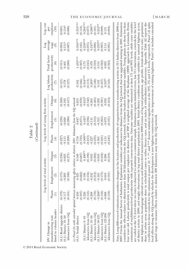
The column headers of Table 2 list dependent variables. Columns 1–3 presentmeasures of total activity, columns 4–6 consider new entrants, columns 7 and 8document productivity outcomes and columns 9 and 10 report wage and labour costmetrics. Panel (a) reports results with a form of specification (1) that only includesinitial values of the outcome variable as a control variable. The first row shows increasesin nodal district activity for all metrics. The higher standard errors of these estimates,compared to the rows beneath them, reflect the fact that there are only nine nodaldistricts. Yet, many of these changes in activity are so substantial in size that one can stillreject that the effect is zero. We do not emphasise these results much, given that theupgrades were built around the connectivity of the nodal cities. Because the bdco-efficients are being measured for each band relative to districts more than50 kilometres from the GQ network, the inclusion or exclusion of the nodal districtsdoes not impact results regarding non-nodal districts.

Our primary emphasis is on the second row where we consider non-nodal districtsthat are 0–10 kilometres from the GQ network. To some degree, the upgrades of theGQ network can be taken as exogenous for these districts. Columns 1–3 find increasesin the aggregate activity of these districts. The co-efficient on output is particularlystrong and suggests a 0.4 log point increase in output levels for districts within10 kilometres of the GQ network in 2007/9 compared to 2000, relative to districtsmore than 50 kilometres from the GQ system. As foreshadowed in Table 1, estimates



Tab

le2

Long-differencedEstimationsof

theIm

pactof

GQ

Improvem

ents,Com

paring2007–9

to2000

DV:Chan

gein

man

ufacturingtrait

listed

inco

lumnheader

Loglevelsoftotalactivity

Loglevelsofyoungfirm

activity

Loglabour

productivity

Totalfactor

productivity

Log

average

wage

Logco

stper

employee

Plants

Employm

ent

Output

Plants

Employm

ent

Output

(1)

(2)

(3)

(4)

(5)

(6)

(7)

(8)

(9)

(10)

(a)Basespatialhorizonmeasuringeffectsrelative

todistricts50+

kilometresfrom

theGQ

network

(0,1)Nodal

district

1.46

7***

1.25

5***

1.41

3***

1.64

0***

2.00

4***

2.46

8***

0.13

81.97

1***

0.38

2***

0.39

3***

(0.496

)(0.464

)(0.480

)(0.499

)(0.543

)(0.621

)(0.111

)(0.195

)(0.065

)(0.069

)(0,1)District0–

10kilometresfrom

GQ

0.36

4***

0.23

50.44

3***

0.81

5***

0.88

2***

1.06

9***

0.19

9***

0.16

30.12

1**

0.13

0**

(0.128

)(0.144

)(0.163

)(0.161

)(0.198

)(0.277

)(0.074

)(0.195

)(0.055

)(0.056

)(0,1)District10

–50

kilometresfrom

GQ

�0.199

�0.325

�0.175

�0.238

�0.087

�0.281

0.15

70.28

60.09

80.09

5(0.185

)(0.222

)(0.293

)(0.237

)(0.314

)(0.455

)(0.126

)(0.280

)(0.091

)(0.094

)

(b)Pan

el(a)includingcovariates

forinitialdistrictconditionsan

dad

ditional

road

andrailroad

traits

(0,1)Nodal

district

0.54

10.46

80.49

30.83

10.96

40.92

70.00

41.36

7***

0.23

9**

0.24

9**

(0.591

)(0.657

)(0.677

)(0.718

)(0.858

)(0.957

)(0.151

)(0.280

)(0.096

)(0.100

)(0,1)District0–

10kilometresfrom

GQ

0.31

2**

0.23

3*0.42

7***

0.61

6***

0.55

5***

0.68

0**

0.24

1***

0.11

20.16

9***

0.18

5***

(0.124

)(0.129

)(0.157

)(0.174

)(0.201

)(0.286

)(0.085

)(0.215

)(0.060

)(0.062

)(0,1)District10

–50

kilometresfrom

GQ

�0.117

�0.202

�0.024

�0.115

�0.025

�0.194

0.17

70.40

30.15

1*0.15

5*(0.161

)(0.196

)(0.271

)(0.207

)(0.279

)(0.416

)(0.127

)(0.288

)(0.087

)(0.090

)

(c)Pan

el(b)includingstatefixedeffects

(0,1)Nodal

district

0.77

30.67

10.66

11.11

01.08

71.03

3�0

.011

1.29

2***

0.25

6**

0.25

9**

(0.643

)(0.718

)(0.728

)(0.797

)(0.963

)(1.062

)(0.157

)(0.342

)(0.114

)(0.117

)(0,1)District0–

10kilometresfrom

GQ

0.33

4**

0.19

40.37

0*0.50

3**

0.36

10.49

00.18

9*0.23

50.16

0**

0.17

7**

(0.147

)(0.172

)(0.211

)(0.208

)(0.246

)(0.345

)(0.113

)(0.262

)(0.073

)(0.075

)(0,1)District10

–50

kilometresfrom

GQ

�0.145

�0.275

�0.147

�0.190

�0.178

�0.382

0.11

30.42

40.12

30.12

6(0.186

)(0.237

)(0.320

)(0.224

)(0.309

)(0.463

)(0.147

)(0.324

)(0.102

)(0.106

)

(d)Pan

el(b)separatingnew

constructionversusimprovem

entsof

existingroads

(0,1)Nodal

district

0.53

90.47

00.48

70.83

30.97

50.92

8�0

.003

1.37

7***

0.24

3**

0.25

3**

(0.594

)(0.659

)(0.681

)(0.720

)(0.860

)(0.961

)(0.153

)(0.281

)(0.096

)(0.101

)(0,1)District0–

10kilometresfrom

GQ

*0.29

5**

0.25

30.38

2**

0.63

6***

0.63

3**

0.69

2**

0.19

4**

0.18

10.19

9***

0.21

1***

(0,1)New

construction

district

(0.129

)(0.156

)(0.171

)(0.203

)(0.258

)(0.332

)(0.083

)(0.197

)(0.065

)(0.066

)

(0,1)District0–

10kilometresfrom

GQ

*0.32

8*0.21

50.46

8**

0.59

8***

0.48

4**

0.66

9*0.28

5**

0.04

60.14

0*0.16

0*



Tab

le2

(Continued)

DV:Chan

gein

man

ufacturingtrait

listed

inco

lumnheader



activity

Loglabour

productivity

Totalfactor

productivity

Log

average

wage

Logco

stper

employee

Plants

Employm

ent

Output

Plants

Employm

ent

Output

(1)

(2)

(3)

(4)

(5)

(6)

(7)

(8)

(9)

(10)

(0,1)Road

upgrad

edistrict

(0.179

)(0.175

)(0.236

)(0.227

)(0.238

)(0.368

)(0.121

)(0.311

)(0.084

)(0.085

)(0,1)District10

–50

kilometresfrom

GQ

�0.117

�0.203

�0.023

�0.115

�0.028

�0.195

0.17

80.40

10.15

1*0.15

4*(0.161

)(0.196

)(0.271

)(0.208

)(0.280

)(0.417

)(0.127

)(0.289

)(0.087

)(0.090

)

(e)Pan

el(b)withextendedspatialhorizonmeasuringeffectsrelative

todistricts200+

kilometresfrom

theGQ

network

(0,1)Nodal

district

0.45

00.42

50.54

90.71

80.84

70.85

30.10

21.43

3***

0.33

4***

0.35

3***

(0.597

)(0.662

)(0.687

)(0.733

)(0.871

)(0.978

)(0.166

)(0.307

)(0.105

)(0.110

)(0,1)District0–

10kilometresfrom

GQ

0.22

60.19

60.49

0**

0.50

9**

0.44

5*0.61

2*0.34

4***

0.17

50.25

9***

0.28

4***

(0.145

)(0.156

)(0.190

)(0.213

)(0.236

)(0.342

)(0.113

)(0.245

)(0.075

)(0.077

)(0,1)District10

–50

kilometresfrom

GQ

�0.208

�0.242

0.04

3�0

.227

�0.141

�0.265

0.28

3*0.47

00.24

7**

0.26

0**

(0.176

)(0.212

)(0.282

)(0.235

)(0.312

)(0.465

)(0.146

)(0.319

)(0.098

)(0.101

)(0,1)District50

-125

kilometresfrom

GQ

�0.268

*�0

.165

�0.043

�0.301

�0.355

�0.292

0.14

30.15

10.23

3**

0.25

2**

(0.150

)(0.173

)(0.242

)(0.221

)(0.265

)(0.391

)(0.167

)(0.322

)(0.097

)(0.099

)(0,1)District12

5-20

0kilometresfrom

GQ

�0.068

0.01

80.28

6�0

.115

�0.072

0.03

20.24

7*0.09

50.11

40.13

1(0.159

)(0.191

)(0.219

)(0.245

)(0.331

)(0.454

)(0.143

)(0.323

)(0.091

)(0.094

)

Notes.L

ong-differencedestimationsco

nsidersch

ange

sin

thelocationan

dproductivityoforgan

ised

-sectorman

ufacturingactivityin

311Indiandistrictsfrom

2000

to20

07–9

from

theAnnual

Survey

ofIndustries.Exp

lanatory

variab

lesareindicators

fordistance

from

theGQ

network

that

was

upgrad

edstartingin

2001

.Estim

ation

considerstheeffectsrelative

todistrictsmore

than

50kilometresfrom

theGQ

network.Columnheaderslist-dep

enden

tvariab

les.Yo

ungplantsarethose

less

than

fouryearsold.Lab

ourproductivityis

totaloutputper

employeein

district,an

dTFPisweigh

tedaverageoftheSivadasan

(200

9)ap

proachto

Levinsohn–P

etrin

estimationsofestablishmen

t-levelproductivitywithrepeatedcross-sectiondata.

Outcomevariab

lesarewinsorisedat

their1%

and99

%levels,whileen

tryvariab

les

areco

ded

atthe1%

levelwherenoen

tryisobserved

tomaintain

aco

nsisten

tsample.E

stim

ationreportsstan

darderrors,h

as31

1observations,co

ntrolsforthelevel

ofdistrictactivity

in20

00,an

dweigh

tobservationsbylogtotaldistrictpopulationin

2001

.Initialdistrictco

nditionsincludevariab

lesfornational

highway

access,

statehighway

access,b

road

-gau

gerailroad

accessan

ddistrict-levelmeasuresfrom

2000

Cen

susoflogtotalpopulation,age

profile,fem

ale-malesexratio,p

opulation

sharein

urban

areas,populationsharein

sched

uledcastes

ortribes,literacy

rates,an

dan

index

ofwithin-districtinfrastructure.Appen

dix

Tab

leA2reportsthe

co-efficien

tsfortheseco

ntrolsfortheestimationin

pan

el(b).*,

**,and**

*den

ote

statisticalsignificance

atthe10

%,5

%an

d1%

levels,respectively.P

anel

(d)splits

localeffectsalongtheGQ

network

bywhether

thedevelopmen

tisnew

highway

constructionortheim

provemen

tofex

istinghighways.Pan

el(e)includes

extended

spatialrings

tomeasure

effectsrelative

todistricts

200kilometresaw

ayfrom

theGQ

network.



for establishment counts and output in districts 0–10 kilometres from the GQ networkexceed the employment responses. These employment effects fall short of beingstatistically significant at a 10% level and this is not due to small sample size as we have76 districts within this range. Generally, the response around the GQ changesfavoured output over employment, which we trace out further below with industry-level analyses.

Columns 4–6 examine the entry margin by quantifying levels of young establish-ments and their activity. We find much sharper entry effects than the aggregate effectsin Columns 1–3 and these entry results are very precisely measured. The districts within0–10 kilometres of GQ have a 0.8–1.1 log point increase in entry activity after the GQupgrade compared to districts more than 50 kilometres away.

Columns 7 and 8 report results for the average labour productivity and TFP in thedistricts 0–10 kilometres from the GQ network. These average values are weighted andthus primarily driven by the incumbent establishments. Labour productivity for thedistrict increases (also evident in a comparison of columns 2 and 3). On the otherhand, we do not observe TFP growth using the Sivadasan (2009) approach andunreported estimations find limited differences between the TFP growth of youngerand older plants (relative to plants of similar ages in the pre-period). This generaltheme is repeated below with continued evidence of limited TFP impact but a strongassociation of the GQ upgrades with higher labour productivity. Columns 9–10 finallyshow an increase in wages and average labour costs per employee in these districts.

For comparison, the third row of panel (a) provides the interactions for the districtsthat are 10–50 kilometres from the GQ network. None of the effects on the allocationof economic activity that we observe in columns 1–6 for the 0–10 kilometres districtsare observed at this spatial band. This isolated spatial impact provides a first assurancethat these effects can be linked to the GQ upgrades rather than other features likeregional growth differences. By contrast, columns 7–10 suggest we should be cautiousabout placing too much emphasis on the productivity and wage outcomes as beingspecial for districts neighbouring the GQ network, since the patterns look prettysimilar for all plants within 50 kilometres of the GQ network. On the other hand, it isimportant to recognise that the productivity/wage growth in columns 7–10 for thedistricts within 10–50 kilometres are coming from relative declines in activity that isevident in columns 1–6. That is, the labour productivity of 0–10 kilometres districts isincreasing because output is expanding more than employment, but in the 10–50 kilometres districts the labour productivity is increasing due to employmentcontracting more than output. The different foundations for the productivity and wagechanges suggest that we should not reject the potential benefits of the GQ network onthese dimensions, and we return to this issue below with a detailed analysis ofproductivity distributions for entrants and incumbents.

The remaining panels of Table 2 test variations on these themes. Panel (b) nextintroduces the longer battery of district traits described above. The inclusion of thesecontrols substantially reduces the co-efficients for the nodal districts. More important,they also diminish somewhat the co-efficients for the 0–10 kilometres districts, yetthese results remain quite statistically and economically important. The controls,moreover, do not explain the differences that we observe between districts 0–10 kilometres from the GQ network and those that are 10–50 kilometres away.



Appendix Table A2 reports the co-efficients for these controls for the estimation inpanel (b). From hereon, this specification becomes our baseline estimate, with futureanalyses also controlling for these district covariates.

Panel (c) further adds in state fixed effects. This is a much more aggressive empiricalapproach than the baseline estimations as it only considers variation within states (andthus we need to have districts located on the GQ network and those farther awaytogether in individual states). This reduces the economic significance of most variablesand raises the standard errors. Yet, we continue to see evidence suggestive of the GQupgrades boosting manufacturing activity.

Panel (d) presents results about the differences in the types of GQ work undertaken.Prior to the GQ project, there was some infrastructure linking these cities. In aminority of cases, the GQ project built highways where none existed before. In othercases, however, a basic highway existed that could be upgraded. Of the 70 districts lyingnear the GQ network, new highway stretches comprised some or all of the constructionfor 33 districts, while 37 districts experienced purely upgrade work. In panel (d), wesplit the 0–10 kilometres interaction variable for these two types of interventions. Theentry results are slightly stronger in the new construction districts, while the labourproductivity results favour the road upgrades. This latter effect is strong enough thatthe total output level grows the most in the road upgrade districts. Despite theseintriguing differences, the bigger message from the breakout exercise is the degree towhich these two groups are comparable overall.

Panel (e) extends the spatial horizons studied in panel (b) to include two additionaldistance bands for districts 50–125 kilometres and 125–200 kilometres from the GQnetwork. These two bands have 48 and 51 districts respectively. In this extendedframework, we measure effects relative to the 97 districts that are more than200 kilometres from the GQ network. Two key observations can be made. First, theresults for districts 0–10 kilometres away are very similar when using the new baseline.Second, the null results generally found for districts 10–50 kilometres from the GQnetwork mostly extend to districts 50–200 kilometres from the GQ network. Even froma simple association perspective, the manufacturing growth in the period surroundingthe GQ upgrades is localised in districts along the GQ network.

It is tempting to speculate that the steeper negative point estimates in columns 4–6suggest a ‘hollowing-out’ of new entry towards districts more proximate to the GQsystem after the upgrades. This pattern would be similar to Chandra and Thompson’s(2000) finding that US counties that were next to counties through which US highwayswere constructed were adversely affected. Chandra and Thompson (2000) describedtheir results within a theoretical model of spatial competition whereby regionalhighway investments aid the nationally oriented manufacturing industries and lead tothe reallocation of economic activity in more regionally oriented industries like retailtrade. Unreported estimations suggest that this local reallocation is not happening forIndian manufacturing, at least in a very tight geographic sense.14 For India, the

14 This exercise considers districts that lie between 10 and 200 kilometres of the GQ network. Using thelong-differenced approach, we regress the change in a district’s manufacturing activity and entry rates on theaverage change in entry rates for the 0–10 kilometres segments within the focal district’s state. There is apositive correlation, which is inconsistent with a ‘hollowing-out’ story operating at a very local level.



evidence is more consistent with potential diversion of entry coming from more distantpoints. Either way, the lack of statistical precision for these estimations prevents strongconclusions in this regard.

Appendix Table A3 provides several robustness checks on these results. We first showvery similar results when not weighting districts and including dropped outlierobservations. We obtain even stronger results on most dimensions when justcomparing the 0–10 kilometres band to all districts more than 10 kilometres apartfrom the GQ network, which is to be expected given the many negative coefficientsobserved for the 10–50 kilometres band. We also show results that include anadditional 10–30 kilometres band. This estimation confirms a very rapid attenuation ineffects. The Appendix also shows similar (inverted) findings when using a lineardistance measure over the 0–50 kilometres range. Appendix Table A4 documentsalternative approaches to calculating labour productivity and TFP consequences.

3.2. Comparison of GQ Upgrades to NS–EW Highway

The stability of the results in Table 2 is encouraging, especially to the degree to whichthey suggest that proximity to the GQ network is not reflecting other traits of districtsthat could have influenced their economic development. There remains someconcern, however, that we may not be able to observe all of the factors that policymakers would have known or used when choosing to upgrade the GQ network anddesigning the specific layout of the highway system. For example, policy makers mighthave known about the latent growth potential of regions and attempted to aid thatpotential through highway development.

We examine this feature by comparing districts proximate to the GQ network todistricts proximate to the NS–EW highway network that was not upgraded. The ideabehind this comparison is that districts that are at some distance from the GQnetwork may not be a good control group if they have patterns of evolution that donot mirror what districts immediately on the GQ system would have experiencedhad the GQ upgrades not occurred. This comparison to the NS–EW corridorprovides perhaps a stronger foundation in this regard, especially as its upgradeswere planned to start close to those of the GQ network before being delayed. Theidentification assumption is that unobserved conditions such as regional growthpotential along the GQ network were similar to those for the NS–EW system(conditional on covariates).

The upgrades scheduled for the NS–EW project were to start contemporaneouslywith and after the GQ project. To ensure that we are comparing apples with apples, weidentified the segments of the NS–EW project that were to begin with the GQ upgradesand those that were to follow in the next phase. We use separate indicator variables forthese two groups so that we can compare against both. Of the 90 districts lying within0–10 kilometres of the NS–EW network, 40 districts were to be covered in the 48 NS–EW projects identified for Phase I. The online Appendix provides greater detail on thisdivision.

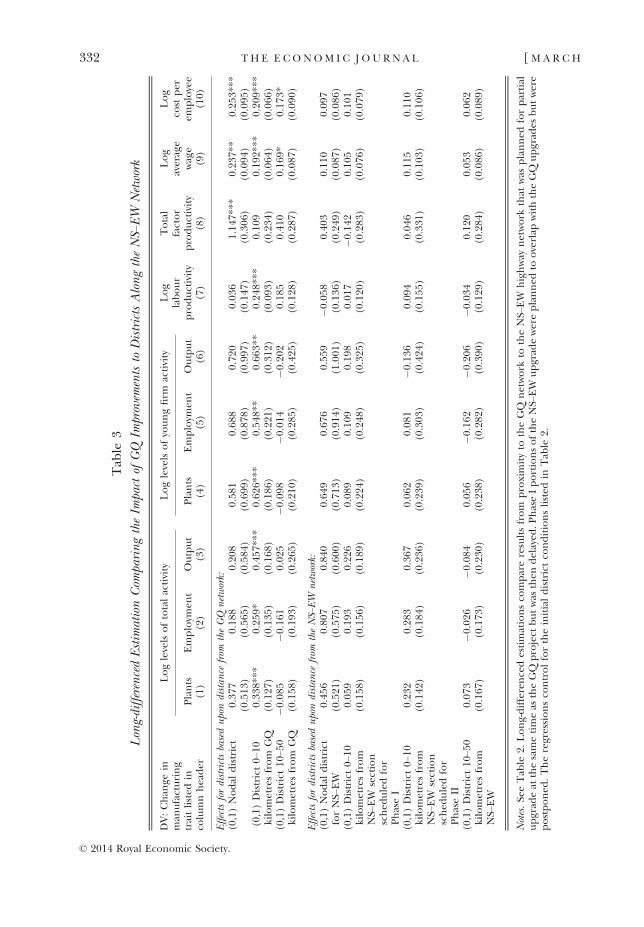
Table 3 repeats panel (b) of Table 2 and adds in four additional indicatorvariables regarding proximity to the NS–EW system and the planned timing ofupgrades. In this estimation, the coefficients are compared to districts more than



Tab

le3

Long-differencedEstimationCom

paringtheIm

pactof

GQ

Improvem

entsto

DistrictsAlongtheNS–EW

Network

DV:Chan

gein

man

ufacturing

traitlisted

inco

lumnheader



activity

Log

labour

productivity

Total

factor

productivity

Log

average

wage

Log

cost

per

employee

Plants

Employm

ent

Output

Plants

Employm

ent

Output

(1)

(2)

(3)

(4)

(5)

(6)

(7)

(8)

(9)

(10)

Effectsfordistrictsbasedupondistan

cefrom

theGQ

network:

(0,1)Nodal

district

0.37

70.18

80.20

80.58

10.68

80.72

00.03

61.14

7***

0.23

7**

0.25

3***

(0.513

)(0.565

)(0.584

)(0.699

)(0.878

)(0.997

)(0.147

)(0.306

)(0.094

)(0.095

)(0,1)District0–

10kilometresfrom

GQ

0.33

8***

0.25

9*0.45

7***

0.62

6***

0.54

8**

0.66

3**

0.24

8***

0.10

90.19

2***

0.20

9***

(0.127

)(0.135

)(0.168

)(0.186

)(0.221

)(0.312

)(0.093

)(0.234

)(0.064

)(0.066

)(0,1)District10

–50

kilometresfrom

GQ

�0.085

�0.161

0.02

5�0

.098

�0.014

�0.202

0.18

50.41

00.16

9*0.17

3*(0.158

)(0.193

)(0.265

)(0.210

)(0.285

)(0.425

)(0.128

)(0.287

)(0.087

)(0.090

)

Effectsfordistrictsbasedupondistan

cefrom

theNS–EW

network:

(0,1)Nodal

district

forNS–

EW

0.45

60.80

70.84

00.64

90.67

60.55

9�0

.058

0.40

30.11

00.09

7(0.521

)(0.575

)(0.600

)(0.713

)(0.914

)(1.001

)(0.136

)(0.249

)(0.087

)(0.086

)(0,1)District0–

10kilometresfrom

NS–

EW

section

sched

uledfor

PhaseI

0.05

90.19

30.22

60.08

90.10

90.19

80.01

7�0

.142

0.10

50.10

1(0.158

)(0.156

)(0.189

)(0.224

)(0.248

)(0.325

)(0.120

)(0.283

)(0.076

)(0.079

)

(0,1)District0–

10kilometresfrom

NS–

EW

section

sched

uledfor

PhaseII

0.23

20.28

30.36

70.06

20.08

1�0

.136

0.09

40.04

60.11

50.11

0(0.142

)(0.184

)(0.236

)(0.239

)(0.303

)(0.424

)(0.155

)(0.331

)(0.103

)(0.106

)

(0,1)District10

–50

kilometresfrom

NS–

EW

0.07

3�0

.026

�0.084

0.05

6�0

.162

�0.206

�0.034

0.12

00.05

30.06

2(0.167

)(0.173

)(0.230

)(0.238

)(0.282

)(0.390

)(0.129

)(0.284

)(0.086

)(0.089

)

Notes.Se

eTab

le2.

Long-differencedestimationsco

mpareresultsfrom

proximityto

theGQ

network

totheNS–

EW

highway

network

that

was

planned

forpartial

upgrad

eat

thesametimeas

theGQ

project

butwas

then

delayed

.PhaseIportionsoftheNS–

EW

upgrad

ewereplanned

tooverlap

withtheGQ

upgrad

esbutwere

postponed

.Theregressionsco

ntrolfortheinitialdistrictco

nditionslisted

inTab

le2.



50 kilometres from both networks. None of the long-differenced outcomes evidentfor districts in close proximity to the GQ network are evident for districts in closeproximity to the NS–EW network, even if these latter districts were scheduled for acontemporaneous upgrade. The placebo-like co-efficients along the NS–EW highwayare small and never statistically significant. The lack of precision is not due to toofew districts along the NS–EW system, as the district counts are comparable to thedistance bands along the GQ network and the standard errors are of very similarmagnitude. The null results continue to hold when we combine the NS–EWindicator variables. Put differently, with the precision that we assess the positiveresponses along the GQ network, we estimate a lack of change along the NS–EWcorridor.

3.3. Straight-line Instrumental Variables Estimation

Continuing with potential identification challenges, a related worry is that perhaps theGQ planners were better able to shape the layout of the network to touch upon India’sgrowing regions (and maybe the NS–EW planners were not as good at this or had areduced choice set). Tables 4 and 5 consider this problem using IV techniques. Ratherthan use the actual layout of the GQ network, we instrument for being 0–10 kilometresfrom the GQ network with being 0–10 kilometres from a (mostly) straight line betweenthe nodal districts of the GQ network.

The identifying assumption in this IV approach is that endogenous placementchoices in terms of weaving the highway towards promising districts (or strugglingdistricts)15 can be overcome by focusing on what the layout would have been if thenetwork was established based upon minimal distances only. This approach relies onthe positions of the nodal cities not being established as a consequence of thetransport network, as the network may have then been developed due to theintervening districts. This is a reverse causality concern and an intuitive example is thedevelopment of cities at low-cost points near to mineral reserves that are accessed byrailway lines. Similar to the straight-line IV used in Banerjee et al. (2012), the fournodal cities of the GQ network were established hundreds or thousands of years ago,making this concern less worrisome in our context.

The exclusion restriction embedded in the straight-line IV is that proximity to theminimum-distance line only affects districts in the post-2000 period due to thelikelihood of the district being on the GQ network and experiencing the highwayupgrade. This restriction could be violated if the districts along these lines possesscharacteristics that are otherwise connected to growth during the post-2000 period. Forexample, these districts could generally have had more-skilled workforces than otherdistricts, and perhaps these educational qualities became more important after 2000.The districts may also have possessed more favourable spatial positions. To guard

15 As Duranton and Turner (2011) highlight, endogenous placement could bias findings in eitherdirection. Infrastructure investments may be made to encourage development of regions with high growthpotential, which would upwardly bias measurements of economic effects that do not control for thisunderlying potential. However, there are many cases where infrastructure investments are made to try to turnaround and preserve struggling regions. They may also be directed through the political process towards non-optimal locations (i.e. ‘bridges to nowhere’). These latter scenarios would downward bias results.



Tab

le4

InstrumentalVariableEstimationUsingDistance

from

aStraight

LineBetweenNodal

Districts

DV:Chan

gein

man

ufacturingtrait

listed

inco

lumnheader



activity

Log

labour

productivity

Total

factor

productivity

Log

average

wage

Log

cost

per

employee

Plants

Employm

ent

Output

Plants

Employm

ent

Output

(1)

(2)

(3)

(4)

(5)

(6)

(7)

(8)

(9)

(10)

(a)BaseOLSestimationthat

excludesnodal

districtsan

dmeasureseffectsrelative

todistricts10+

kilometresfrom

theGQ

network

(0,1)District0–

10kilometresfrom

GQ

0.36

2***

0.26

4*0.45

8***

0.84

0***

0.88

1***

1.10

0***

0.17

4**

0.11

60.10

4*0.11

5**

(0.122

)(0.139

)(0.158

)(0.156

)(0.191

)(0.270

)(0.070

)(0.186

)(0.053

)(0.054

)

(b)Reduced-form

estimates

fordistan

cefrom

astraight-linebetweennodal

districts

(0,1)District0–

10kilometres

from

lineROUTE1

0.16

8�0

.015

0.25

60.40

6**

0.31

00.35

80.25

3***

0.13

20.14

6**

0.16

2***

(0.122

)(0.136

)(0.168

)(0.176

)(0.218

)(0.310

)(0.085

)(0.210

)(0.061

)(0.062

)

(0,1)District0–

10kilometres

from

lineROUTE2

0.19

50.05

60.31

5*0.45

0**

0.41

8*0.44

80.22

0***

0.31

90.17

5***

0.18

6***

(0.123

)(0.139

)(0.170

)(0.179

)(0.221

)(0.312

)(0.085

)(0.199

)(0.059

)(0.060

)

(c)IV

estimates

usingdistan

cefrom


districts

(0,1)District0–

10kilometres

from

lineROUTE1

0.34

3�0

.030

0.51

30.81

8**

0.62

20.71

30.49

0***

0.25

60.28

2**

0.31

3**

(0.236

)(0.280

)(0.322

)(0.323

)(0.408

)(0.585

)(0.172

)(0.405

)(0.122

)(0.125

)Exo

geneity

test

p-value

0.92

80.20

70.85

30.94

70.49

80.48

70.03

90.71

40.08

30.05

8

(0,1)District0–

10kilometres

from

lineROUTE2

0.32

0*0.09

20.50

9*0.72

6***

0.67

5**

0.71

70.34

8**

0.50

30.27

6***

0.29

4***

(0.193

)(0.226

)(0.266

)(0.259

)(0.330

)(0.471

)(0.136

)(0.316

)(0.098

)(0.100

)Exo

geneity

test

p-value

0.79

10.33

60.82

40.64

40.48

30.37

10.15

10.16

10.02

80.02

4

Notes.Se

eTab

le2.

Pan

el(a)modifies

thebaseOLSestimationto

excludenodal

districts

andmeasure

effectsrelative

todistricts

10+kilometresfrom

theGQ

network.Thissample

contains30

2districts.Pan

el(b)reportsreduced-form

estimationofwhether

ornotadistricted

geiswithin

10kilometresofastraightline

betwee

nnodal

districts.Pan

el(c)reportsIV

estimationthat

instrumen

tsbeingwithin

10kilometresfrom

theGQ

network

withbeingwithin

10kilometresofthe

straightlinebetweennodal

districts.Route

1does

notco

nnectBan

galore

directly,withthefirst-stageelasticity

of0.43

(0.05)

andtheassociated

F-statistic

of74

.5.

Route

2treats

Ban

galore

asaco

nnection

point,

with

thefirst-stageelasticity

of0.54

(0.05)

and

theassociated

F-statistic

of13

8.1.

Thenullhypothesis

inthe

exoge

neity

testsisthat

theinstrumen

tedregressorisex

oge

nous.



Tab

le5

Table4IncludingDistrictControls

DV:Chan

gein

man

ufacturing

traitlisted

inco

lumnheader



activity

Log

labour

productivity

Total

factor

productivity

Log

average

wage

Log

cost

per

employee

Plants

Employm

ent

Output

Plants

Employm

ent

Output

(1)

(2)

(3)

(4)

(5)

(6)

(7)

(8)

(9)

(10)


excludesnodal

districtsan


todistricts10+

kilometresfrom

theGQ

network

(0,1)District0–

10kilometresfrom

GQ

0.31

9***

0.24

6**

0.38

1**

0.62

8***

0.54

1***

0.66

3**

0.18

6**

0.03

00.12

0**

0.13

6**

(0.117

)(0.123

)(0.150

)(0.172

)(0.197

)(0.279

)(0.076

)(0.203

)(0.057

)(0.058

)

(b)Reduced-form

estimates

fordistan

cefrom


districts

(0,1)District0–

10kilometres

from

lineROUTE1

0.16

50.01

60.27

5*0.29

8*0.10

60.12

50.29

9***

0.18

30.18

5***

0.20

4***

(0.112

)(0.114

)(0.155

)(0.165

)(0.201

)(0.291

)(0.096

)(0.212

)(0.065

)(0.066

)

(0,1)District0–

10kilometres

from

lineROUTE2

0.15

30.04

60.26

40.27

60.10

10.05

10.25

0***

0.32

70.20

9***

0.22

5***

(0.116

)(0.118

)(0.162

)(0.175

)(0.211

)(0.300

)(0.096

)(0.204

)(0.065

)(0.067

)

(c)IV

estimates

usingdistan

cefrom


districts

(0,1)District0–

10kilometres

from

lineROUTE1

0.37

40.03

80.62

3*0.66

7*0.23

90.28

00.66

0***

0.40

20.40

9***

0.45

2***

(0.238

)(0.256

)(0.339

)(0.344

)(0.434

)(0.635

)(0.225

)(0.464

)(0.153

)(0.157

)Exo

geneity

test

p-value

0.80

30.38

20.47

40.90

50.45

70.53

60.01

90.40

80.02

60.01

6

(0,1)District0–

10kilometres

from

lineROUTE2

0.27

40.08

30.47

1*0.48

5*0.17

90.08

90.43

8**

0.57

10.36

8***

0.39

5***

(0.197

)(0.208

)(0.279

)(0.285

)(0.360

)(0.519

)(0.171

)(0.364

)(0.122

)(0.124

)Exo

geneity

test

p-value

0.79

30.37

60.73

90.57

30.25

20.23

30.11

30.10

30.01

40.01

1

Notes.S

eeTab

le4.

Estim

ationincludes

districtco

ntrolsfrom

pan

el(b)ofTab

le2other

than

road

andrailroad

accessvariab

les.Route

1does

notco

nnectBan

galore

directly,withafirst-stageelasticity

of0.38

(0.05)

andassociated

F-statistic

of13

.9.Route

2treatsBan

galore

asaco

nnectionpoint,withafirst-stageelasticity

of0.49

(0.05)

andassociated

F-statistic

of20

.9.



against these concerns, we will estimate the IV with and without the battery ofcovariates for district traits in 2000.16

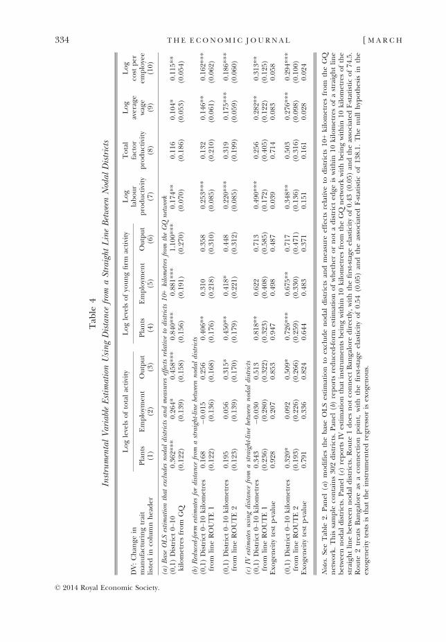
Panel (b) of Figure 1 shows the implementation. IV Route 1 is the simplest approach,connecting the four nodal districts outlined in the original Datta (2011) study. Weallow one kink in the segment between Chennai and Kolkata to keep the straight lineon dry land. IV Route 1 overlaps with the GQ layout and is distinct in places. We earliermentioned the question of Bangalore’s treatment, which is not listed as a nodal city inthe Datta (2011) work. Yet, as IV Route 2 shows, thinking of Bangalore as a nodal city isvisually compelling. We thus test two versions of the IV specification, with and withoutthe second kink for Bangalore.

Panel (a) of Table 4 provides a baseline OLS estimation similar to panel (a) of Table2. For this IV estimation, we drop nodal districts (sample size of 302 districts) andmeasure all effects relative to districts more than 10 kilometres from the GQ network.This approach only requires us to instrument for a single variable – being within10 kilometres of the GQ network. Panel (b) shows the reduced-form estimates, with thecoefficient for each route being estimated from a separate regression. The reduced-form estimates resemble the OLS estimates for many outcomes.

The first-stage relationships are quite strong. IV Route 1, which does not connectBangalore directly, has a first-stage elasticity of 0.43 (0.05) and an associated F-statisticof 74.5. IV Route 2, which treats Bangalore as a connection point, has a first-stageelasticity of 0.54 (0.05) and an associated F-statistic of 138.1. Panel (c) presents thesecond-stage results. Not surprisingly, given the strong fit of the first-stage relationshipsand the directionally similar reduced-form estimates, the IV specifications generallyconfirm the OLS findings. In most cases, we do not statistically reject the nullhypothesis that the OLS and IV results are the same. Wage and labour productivity arethe two exceptions, where the IV indicates that OLS underestimates the true impact.

In Table 5, we repeat this analysis and further introduce the district covariatesmeasured in 2000 that we modelled in panel (b) of Table 2.17 When doing so, the first-stage retains reasonable strength. IV Routes 1 and 2 have associated F-statistics of 13.9and 20.9 respectively. The covariates have an ambiguous effect on the reduced-formestimates, being very similar for aggregate outcomes, generally lower for entry growth,and generally higher for productivity and wage effects. Most results carry through,although the second-stage coefficients for employment and output entry aresubstantially lower. Among the controls added, the inclusion of the total populationcontrol is the most important for explaining differences between Tables 4 and 5. Weagain do not statistically reject the null hypothesis that the OLS and IV results are the

16 Banerjee et al. (2012) provide an early application and discussion of the straight-line IV approach, andKhanna (2014) offers a recent application to India. Faber (2014) provides an important extension to thismethodology. Faber (2014) uses data on local land characteristics and their impact on construction costs todefine a minimum-cost way of connecting 54 key cities that were to be linked by the development of China’shighway network. We do not replicate Faber’s (2014) approach due to our focus on particular segments ofIndia’s network and the difficulty assembling the very detailed geographic data necessary for calculatingminimum-cost paths (versus minimum distance). We hope in future research to examine the whole system ofIndia’s highway network similar to Faber (2014).

17 We do not include in these estimates the three road and railroad access metrics variables, since these aremeasured after the reform period, and we want everything in this analysis to be predetermined. Thesevariables can be included, however, with little actual consequence for Table 5’s findings.



same for most outcomes. We obtain similar outcomes when also including controls fordistance from India’s 10 largest cities.

On the whole, we find general confirmation of the OLS findings with these IVestimates, which help with particular concerns about the endogenous weaving of thenetwork towards certain districts with promising potential. IV estimates indicate thatthere may be an upward bias in the entry findings, perhaps due to endogenousplacement towards districts that could support significant new plants in terms ofoutput. A second alternative is that the GQ upgrades themselves had a particularfeature that accentuates these metrics (e.g. high output levels of contracted plants tosupport the actual construction of the road). This latter scenario seems unlikely,however, given the industry-level patterns documented below.

3.4. Dynamic Specifications

Dynamicpatternsaroundthesereformsprovideadditionalassuranceabout theroleof theGQ upgrades in these economic outcomes and insight into their timing. A first step is toestimate our basic findings in a pre–post format. We estimate this panel regression usingnon-nodaldistrictswithin50 kilometresof theGQnetwork.Wethusestimateeffects for0–10 kilometres districts compared to those 10–50 kilometres apart from the GQhighways.18 Indexingdistrictswith i andtimewith t, thepanel specification takes theform:

Yi;t ¼ b� ð0; 1ÞGQDisti;d\10km � ð0; 1ÞPostGQt þ /i þ gt þ ei;t : (2)

The distance indicator variable takes unit value if a district is within 10 kilometres ofthe GQ network and the PostGQt indicator variable takes unit value in the years 2001and afterwards. The panel estimations include a vector of district fixed effects /i and avector of year fixed effects gt . The district fixed effects control for the main effects ofdistance from the GQ network, and the year fixed effects control for the main effects ofthe post-GQ upgrades period. Thus, the b coefficient quantifies differences inoutcomes after the GQ upgrades for those districts within 10 kilometres of the GQnetwork compared to those 10–50 kilometres away.

Table 6 implements this approach using the 1994, 2000, 2005, 2007 and 2009 data.These estimates cluster standard errors by district, weight districts by log population in2001 and include 530 observations from the cross of five periods with 106 districtswhere manufacturing plants, employment and output are continually observed in allfive surveys. The results are quite similar to the earlier work, especially for the entryvariables. The total activity variables in columns 1–3 are somewhat diminished,however, and we later describe the time path of the effects that is responsible for thisdeviation. The productivity and wage estimations show weaker patterns, which is to beexpected, given how close the two bands looked in Table 2’s analysis. We report themfor completeness but we do not discuss their dynamics further.19

18 We will be interacting these distance variables with annual metrics, and the reduced set of coefficients isappealing. Our NBER working paper (Ghani et al. 2013) contains earlier results that show similar patternswhen several distance bands are interacted with time variables.

19 Our young plant variables recode entry to the 1% observed value by year if no entry activity is recordedin the data. The 1% value is the winsorisation level generally imposed. Appendix Table A5 shows similarresults when using a negative binomial estimation approach to model plants and employments as countvariables where zero values have meaning.



Tab

le6

Estimationof

theIm

pactof

GQ

Improvem

entsby

Com

pletionDate,Districtswithin50kilometresof

GQ

Network

DV:Chan

gein

man

ufacturingtrait

listed

inco

lumn

header



activity

Log

labour

productivity

Total

factor

productivity

Log

average

wage

Log

cost

per

employee

Plants

Employm

ent

Output

Plants

Employm

ent

Output

(1)

(2)

(3)

(4)

(5)

(6)

(7)

(8)

(9)

(10)

(a)Baseestimationmeasuringeffectsrelative

todistricts10–5

0kilometresfrom

theGQ

network

(0,1)Post

GQ

upgrad

es9

0.18

40.19

00.37

60.58

1**

0.54

11.02

1**

0.18

5�0

.016

0.01

50.04

9(0,1)District0–

10kilometres

from

GQ

(0.154

)(0.182

)(0.244

)(0.243

)(0.355

)(0.509

)(0.117

)(0.147

)(0.087

)(0.096

)

(b)Pan

el(a)usingtimingof

GQ

sectioncompletions

(0,1)Post

GQ

upgrad

es9

0.20

90.29

50.41

40.68

9**

0.68

0*1.16

2**

0.11

1�0

.114

0.03

60.04

2(0,1)District0–

10kilometres

from

GQ

andco

mpletedby

March

2003

(0.192

)(0.215

)(0.288

)(0.277

)(0.400

)(0.585

)(0.146

)(0.166

)(0.098

)(0.103

)

(0,1)Post

GQ

upgrad

es9

0.21

80.20

30.35

70.57

1*0.54

90.91

60.15

30.05

1�0

.040

0.00

6(0,1)District0–

10kilometres

from

GQ

andco

mpleted

2003

–200

6

(0.196

)(0.223

)(0.285

)(0.301

)(0.410

)(0.593

)(0.131

)(0.146

)(0.104

)(0.111

)

(0,1)Post

GQ

upgrad

es9

0.07

7�0

.027

0.34

00.39

90.27

40.95

20.37

5***

0.03

90.07

60.14

1(0,1)District0–

10kilometres

from

GQ

andco

mpletedafter

March

2006

(0.212

)(0.232

)(0.325

)(0.380

)(0.518

)(0.700

)(0.141

)(0.279

)(0.121

)(0.133

)

Notes.S

eeTab

le2.

Estim

ationco

nsidersthelocationan


ised

-sectorman

ufacturingactivityin

non-nodalIndiandistrictswithin

50kilometresof

theGQ

network

for19

94,20

00,20

05,20

07an

d20

09from

theAnnual

Survey

ofIndustries.Pan

el(a)repeats

thebasespecification

inthenarrower

range

.Estim

ationin

pan

el(b)separates

upgrad

esbyco

mpletiondate.

Estim

ationreportsstan

darderrors

clustered

bydistrict,includes

districtan

dyear

fixe

deffects,with

530observationsan

dobservationsweigh

tedbylogtotaldistrictpopulationin

2001

.



Panel (b) studies the actual completion dates of the GQ upgrades. Due to the size ofthe GQ project, some sections were completed earlier than other sections. We modelthis by extending the 0–10 kilometres indicator variable so it also reflects whether thedistrict’s work was completed by March 2003 (27 districts), between March 2003 andMarch 2006 (27 districts) or later (16 districts). Columns 1–6 find that the relative sizesof the effects by implementation date are consistent with the project’s completiontaking hold and influencing economic activity. The results are strongest for sectionscompleted by March 2003, closely followed by those sections completed by March 2006.On the other hand, there is a drop-off in many findings for the last sections completed.

Figure 2 further extends specification (2) to take a non-parametric dynamic format:

Yi;t ¼X

t2Tbt � ð0; 1ÞGQDisti;d\10km � ð0; 1ÞYeart þ /i þ gt þ ei;t : (3)

Rather than introduce post-GQ upgrades variables, we introduce separate indicatorvariables for every year starting with 1999. We interact these year indicator variableswith the indicator variable for proximity to the GQ network. The vectors of district andyear fixed effects continue to absorb the main effects of the interaction terms. Thus,

1999

2000

2001

2002

2003

2004

2005

2006

2007

2008

2009

1999

2000

2001

2002

2003

2004

2005

2006

2007

2008

2009

1999

2000

2001

2002

2003

2004

2005

2006

2007

2008

2009

1999

2000

2001

2002

2003

2004

2005

2006

2007

2008

2009

2.0

1.5

80%Complete

1.0

0.5

0.0

0.0

1.0

1.5

–1.0–0.50.00.51.01.52.02.53.0

0.0

0.2

–0.2–0.4–0.6 –0.5

0.5

–0.8–1.0 –1.0

0.40.60.8

Dynamics of Log New Plant Growth Dynamics of Log New Output Growth

Dynamics of Log Total Output GrowthDynamics of Log Total Plant Growth

GQUpgradesStart

80%Complete

GQUpgradesStart

80%Complete

GQUpgradesStart

80%Complete

GQUpgradesStart

–0.5

–1.0

(a) (b)

(c) (d)

Fig. 2. Dynamics of Plant Count and Output Growth Around the GQ UpgradesNotes. Panels (a) and (c) illustrate the dynamics of young entrant and total plant count growth fornon-nodal districts located 0–10 kilometres from the GQ network relative to districts 10–50 kilometres from the GQ network. The solid line quantifies the differential effect for the GQupgrades by year, with 1994 as the reference year. Dashed lines present 90% confidence intervals,with standard errors clustered by district. Panels (b) and (d) consider comparable outputestimations. Appendix Table A6 reports complete regression results.



the bt coefficients in specification (3) quantify annual differences in outcomes for 0–10 kilometres districts compared to those 10–50 kilometres away, with 1994 serving asthe reference period. This estimation includes 1,188 observations as the cross of12 years with the 99 non-nodal districts within 50 kilometres of the GQ network forwhich we can always observe their activity.

By separately estimating effects for each year, we can observe whether the growthpatterns appear to follow the GQ upgrades hypothesised to cause them. Conceptually,we also believe this dynamic approach is a better way of characterising the impact ofthe GQ upgrades than the specific completion dates of segments. Once the upgradesstarted, work began all along the GQ network and proceeded in parallel. Every statealong the GQ network had at least one segment completed within the first two years ofthe programme. Work continued thereafter across all states, with the average spread ofcompletion times between the first and last segments for states being 6.4 years. Sincemanufacturing activity and location choice decisions can easily be influenced byupgrades on nearby segments (and even anticipation of future upgrades to a segment),we believe it more appropriate to model the GQ event as a whole, timing the impact ofall segments from 2001.

Panels (a) and (b) of Figure 2 plot the coefficient values for log entrant counts andlog new output, respectively, and their 90% confidence bands. These panels includevertical lines to mark when the GQ upgrades began and when they reached the 80%completion mark. The entrant patterns are pretty dramatic. Effects are measuredrelative to 1994 and we see no differences in 1999 or 2000 for non-nodal districts within10 kilometres of the GQ compared to those 10–50 kilometres apart for either entrantmeasure. Once the GQ upgrades commence, the log entry counts in neighbouringdistricts outpace those a bit farther away. These gaps increase throughout the periodand are statistically significant in 2004 and 2009. In panel (b), output rises moredramatically and increases up until the upgrades are mostly complete. The differencesbegin to diminish in 2005 and then stabilise for 2006–9. New output (andemployment) growth substantially lead the new establishment effects, a patternreflective of large plants being the earliest to respond to the GQ upgrades.

Panels (c) and (d) show the series for log total plant counts and output. Aggregateplant counts are very stable before the upgrades start. There is some measure of adownward trend in output levels for 0–10 kilometres districts before the reform, butthese pre-results are not statistically different from each other nor from 1994 levels.After the GQ upgrades start, total plant counts and output also climb and thenstabilise, before climbing again as the sample period closes. At all points during thispost period, the coefficient values are positive, indicating an increase over 1994 levels,but the differences are not statistically significant until the end.

The paths depicted in these Figures provide important insights. The young entrantmeasures in panels (a) and (b) are in essence flow variables into the district. Thus,comparing the post-2006 period to 2004, it is not that the earlier cohort of young firmsis shrinking. Instead, a surge of entry occurred as the GQ upgrades made areas moreaccessible and, with time, this surge abated into a lower sustained entry rate that stillexceeded pre-reform levels. By contrast, the metrics in panels (c) and (d) are stockvariables. Thus, their gradual development over time as more entrants come in and thelocal base of firms expands makes intuitive sense.



We began in Table 2 by considering long-differenced specifications that compareactivity in 2000 with 2007/9. Figure 2 and the Appendix material highlight the positionof these long-differenced years.20 The choice of 2000 as a base year is theoreticallyappropriate as it is immediately before the upgrades began. This choice, however, isnot a sensitive point for the analysis. Utilising 1994 or 1999 delivers a very similarbaseline, while the 2001 period would generally lead to larger effects due to the dip insome variables. To this end, the Appendix shows that the downward shift in output inFigure 2 is by far the largest pre-movement among the outcomes considered.Encouragingly, there is no evidence of a pre-trend that upward biases our work withany outcome variable.

The choice of averaging 2007 and 2009 is also illuminated. The dynamics of mostaggregate outcomes provide a similar picture to Figure 2. The common themes are ageneral increase in activity across the post-2002 period, with individual years notstatistically significant, and then a run-up as 2009 approaches. By averaging 2007 and2009, we give a better representation of the aggregate impact than using 2009 alone.The entry margin – where location choices are being made at present – adjusts muchfaster to the changing attractiveness of regions and thus registers sharper effects in theshort to medium-run. We return to projections about future impacts from the GQupgrades in the closing Section.

3.5. Entrants and Incumbents

Plant-level data offer the opportunity to examine the roles of entrants and incumbentsin aggregate growth – whether the growth is mainly through the displacement of olderplants by new entrants, within-plant productivity growth, or some combination of thetwo. The ideal scenario for this analysis is to have panel data on plants (Glaeser et al.2014). While we unfortunately lack this panel structure, we can use information on theages of plants to consider cohorts over time.

Columns 1–3 of Table 7 consider the role of incumbents in this growth by estimatingthe log activity in 2007/9 due to plants that have been alive at least 10 years comparedto the total initial activity of the district in 2000. The positive coefficient in column 1for the 0–10 kilometres group suggests that a greater fraction of the firms alreadypresent in the 0–10 kilometres districts by 2000 (i.e. before the GQ upgrades began)survived to 2007/9 than firms in their peer cohorts in districts farther away from theGQ network. Columns 2 and 3 further show that employment and output increaseddisproportionately for these incumbent firms. Moreover, the relative magnitudesof columns 1–3 emphasise a point made earlier about the productivity results. For the0–10 kilometres districts, output is rising at a faster pace than employment, leadingtowards higher labour productivity at the same time that plant survival is also growing.By contrast, incumbents in the 10–50 kilometres districts are closing at a similar rate oreven faster than the control group. These more-distant plants are also sheddingemployment faster than output. As a result, their labour productivity is also rising but

20 Appendix Table A6 documents dynamic estimations for all of our outcome variables. Appendix TableA7 also provides comparable results that utilise time since segment completion on an annual basis.



Tab

le7

Long-differencedEstimationof

theRelativeRoleof

IncumbentsversusEntran

tsin

Districts

Loglevelsofactivityin

2007

/9dueto

incu

mben

tsaliveforat

least10

years

compared

tototalinitialdistrict

activity

in20

00

Loglevelsofactivity

in20

07/9dueto

firm

sless

than

10yearsold

compared

tototalinitialdistrictactivity

in20

00

Shareofactivity

in20

07/9in

district

that

isco

ntained

inincu

mben

tplants

atleast10

yearsin

age

Plants

Employm

ent

Output

Plants

Employm

ent

Output

Plants

Employm

ent

Output

(1)

(2)

(3)

(4)

(5)

(6)

(7)

(8)

(9)

(0,1)Nodal

district

0.30

20.25

20.26

60.92

60.79

30.82

70.01

6�0

.010

0.11

3(0.569

)(0.645

)(0.690

)(0.938

)(1.043

)(1.058

)(0.136

)(0.077

)(0.356

)(0,1)District0–

10kilometresfrom

GQ

0.22

0*0.21

60.45

1***

0.71

0***

0.63

3***

0.83

0***

�0.282

***

�0.136

***

�0.282

(0.121

)(0.137

)(0.161

)(0.206

)(0.244

)(0.295

)(0.074

)(0.052

)(0.250

)(0,1)District10

–50kilometresfrom

GQ

�0.130

�0.232

�0.035

�0.284

�0.366

�0.477

�0.101

�0.033

�0.151

(0.189

)(0.228

)(0.311

)(0.354

)(0.434

)(0.472

)(0.087

)(0.051

)(0.177

)

Notes.Se

eTab

le2.

Estim

ationco

mpares

activity

amongincu

mben

tsan

den

tran

tsin

districtsalongtheGQ

network.Totalactivity

forthedistrictin

2000

istake

nas

thebaselineforallestimation.Columns1–

3co

mparetheloglevelsofactivity

infirm

sat

least10

yearsold

in20

07/9to

the20

00baseline.

Positive

values

indicate

relatively

higher

survival

and/orwithin-firm

growth.Columns4–

6co

mparetheloglevelsofactivity

infirm

sless

than

10yearsold

in20

07/9to

the20

00baseline.

Positive

values

indicategreateraccu

mulateden

tryat

theen

dofthesample

period.Columns7–

9co

nsider

astheoutcomevariab

letherawshareofactivity

among

older

incu

mben

tfirm

s.Estim

ationincludes

theco

variates

forinitialdistrictco

nditionsan

dad

ditional

road

andrailroad

traits

usedin

pan

el(b)ofTab

le2.



the origin of this productivity growth is very different from that in the districts near tothe GQ network.

Columns 4–6 quantify the role of entrants by considering as the outcome variablethe log activity in 2007/9 due to plants that have been alive fewer than 10 yearscompared to the total initial activity of the district in 2000. This young firm activity ismeasured against the same baseline as in columns 1–3 but it is important to note thatthe relative co-efficient sizes measure proportionate effects and thus do not directlyrank order aggregate effects (further discussed in the closing Section). The outcomemeasures are all very strong for the 0–10 kilometres districts. There is also someevidence suggestive of larger entrants being less likely to locate in the 10–50 kilometresband.

Thus, both entrants and incumbents contribute to the aggregate growth evident inTable 2. The last three columns consider as an outcome variable the share of activity ineach district in 2007/9 contained in firms that have been alive 10 or more years.Despite their better survival rates and growth compared to distant incumbent peers,the share of activity accounted for by incumbent firms in districts along the GQnetwork declines.21

Table 8 further analyses the productivity distributions and selection margins indistricts by distance from the GQ network. We first normalise the plant-levelproductivity estimates developed using the Sivadasan (2009) methodology by dividingby the employment-weighted average productivity estimate for an industry-year. Wethen calculate in column 1 the average normalised TFP in 2000 for plants withindistricts by distance from the GQ network. These entries sum over all industries andplants within each district group, weighting individual observations by employmentlevels. Normalised productivity levels are naturally centred on one and are somewhathigher in nodal districts – a typical finding in urban productivity patterns – with thefurther initial differences over the other distance bands being marginal.

Column 2 provides a similar calculation in 2007/9. The normalisation process againcentres values on one, such that aggregate TFP growth is removed at the industry level.The percentage listed next to each entry in column 2 is the average value in 2007/9compared to that in 2000. Overall, there is limited movement for any of the groups; the0–10 kilometres range increases slightly, while the other three ranges show very smalldeclines. This pattern is possible because the 0–10 kilometres group is becominglarger during the period of study.

The more interesting tabulations are in columns 3 and 4. In column 3, we calculatethese TFP averages for plants that are at least 10 years old in 2007/9, while column 4presents the comparable figures for plants less than 10 years old. Productivity rises with

21 We find similar results if grouping firms by whether or not they were specifically alive in 2000 but the10-year bar on firm age allows us to apply a consistent threshold across the 2007 and 2009 surveys. In a smallnumber of districts, activity is not observed for either entrants or incumbents (but at least one group is alwaysobserved). In these cases, we recode the zero value in 2007/9 with the lowest observed proportion amongdistricts with reported data on that margin. That is, if the lowest observed incumbent employment proportionis 5% of the initial 2000 district size, we use this 5% estimate for the districts where zero incumbents areobserved. This approach maintains a consistent sample. We find very similar results when excluding thesecases, with the one change being that the output contributions of incumbents and entrants becomesubstantially closer in size.



plant age, such that the values in column 3 are higher than in column 4. This may bedue to differences in technical efficiency. As pointed out in Foster et al. (2008), thesedifferences could also result from using revenues for TFP calculations rather thanphysical products, if, for example young firms have lower prices to build demand.Either way, our focus is on the relative comparisons back to the initial 2000 period thatare expressed in the accompanying percentages.

Column 3 shows that surviving incumbent plants in the 10–50 kilometres rangefrom the GQ network have substantially higher TFP compared to initial values than inthe other district ranges. These districts have reduced entry rates and the entrantshave lower TFPs compared to the other bands. By contrast, the TFP distributions forthe 0–10 districts have a more homogeneous adjustment over entrants and incum-bents. The stability in entrant TFP in these districts is important, given the massiveincrease in entry rates associated with the GQ upgrades. Despite these surges, the TFPpositions are not weakening compared to districts that are 50 kilometres or more fromthe GQ network. This comparison shows again the very different sources ofproductivity development in the 0–10 kilometres versus 10–50 kilometres rangessurrounding the GQ network with the upgrades.

3.6. District and Industry Heterogeneity

The remaining analyses quantify heterogeneity in effects for districts and industries.Table 9 considers district heterogeneity using the long-differenced specification (1).Articulating this heterogeneity is challenging empirically because the data variationbecomes very thin as one begins to partition the sample by additional traits beyondproximity to the GQ network. We take a simple approach by allowing the coefficient on0–10 kilometres districts to vary by whether the district is above or below the median

Table 8

Productivity Distributions Among Incumbents and Entrants

Average ofnormalisedTFP metricin 2000

Average ofnormalisedTFP metricin 2007/9

Average ofnormalised TFPmetric in 2007/9,Plants 10+ years

old

Average ofnormalised TFPmetric in 2007/9,Plants less than

10 years(1) (2) (3) (4)

Nodal district for GQ 1.0349 1.0274, 99% 1.0344, 100% 1.0096, 98%District 0–10 kilometres from GQ 0.9998 1.0011, 100% 1.0068, 101% 0.9797, 98%District 10–50 kilometres from GQ 1.0044 1.0038, 100% 1.0346, 103% 0.9006, 90%District 50+ kilometres from GQ 0.9915 0.9912, 100% 0.9982, 101% 0.9654, 97%

Notes. Normalised TFP metrics divide plant-level TFP values developed with the Sivadasan (2009) approach bytheir industry-year average value (weighted by employment in plant). Entries on the table are thenemployment-weighted averages over these normalised metrics across all plants located in the indicateddistricts (aggregating all districts and industries). Column 1 reports initial values in 2000. Column 2 reportsaverages in 2007/9 and their relative percentage ratio to 2000. Column 3 reports the value for plants at leastten years of age and their ratio to the initial value in 2000. Column 4 reports a similar statistic for subsequententrants and their ratio to the initial value in 2000. Districts in the 10–50 kilometres show a very strongselection effect towards incumbent plants, while districts in the 0–10 kilometres range show morehomogeneous adjustments over entrants and incumbents.



Tab

le9

InteractionswithDistrictTraits

DV:Chan

gein

man

ufacturing

traitlisted

inco

lumnheader



activity

Log

labour

productivity

Total

factor

productivity

Log

average

wage

Log

cost

per

employee

Plants

Employm

ent

Output

Plants

Employm

ent

Output

(1)

(2)

(3)

(4)

(5)

(6)

(7)

(8)

(9)

(10)


excludesnodal

districtsan


todistricts10–5

0kilometresfrom

theGQ

network

(0,1)District0–

10kilometres

from

GQ

0.49

0**

0.50

1**

0.58

3**

1.01

7***

0.93

2***

1.34

3***

0.02

0�0

.128

0.01

60.03

0(0.205

)(0.234

)(0.284

)(0.265

)(0.327

)(0.480

)(0.126

)(0.292

)(0.093

)(0.096

)(b)Pan

el(a)withinteractionsplitusingmedianof

districtpopu

lation

density

(0,1)District0–

10kilometres

from

GQ–A

bove

med

ian

0.75

6***

0.80

7***

0.82

5***

1.26

9***

1.31

1***

1.78

4***

0.01

00.12

20.08

40.10

2(0.243

)(0.275

)(0.286

)(0.312

)(0.349

)(0.492

)(0.130

)(0.309

)(0.098

)(0.100

)(0,1)District0–

10kilometres

from

GQ–M

edianvalue

andbelow

0.32

30.31

50.40

50.83

2***

0.66

3*0.99

2*0.03

0�0

.382

�0.055

�0.044

(0.229

)(0.268

)(0.359

)(0.294

)(0.373

)(0.557

)(0.141

)(0.341

)(0.104

)(0.107

)

(c)Pan


districtliteracy

(0,1)District0–

10kilometres

from

GQ–A

bove

med

ian

0.51

4**

0.77

6***

0.84

8***

1.09

2***

1.27

3***

1.87

5***

0.06

00.19

90.11

50.13

4(0.232

)(0.264

)(0.299

)(0.299

)(0.334

)(0.485

)(0.127

)(0.301

)(0.098

)(0.100

)(0,1)District0–

10kilometres

from

GQ–M

edianvalue

andbelow

0.46

9**

0.27

30.33

10.94

0***

0.60

20.78

3�0

.032

�0.546

�0.116

�0.108

(0.236

)(0.269

)(0.354

)(0.289

)(0.386

)(0.564

)(0.147

)(0.354

)(0.104

)(0.109

)

(d).Pan


districtinfrastructure

index

(0,1)District0–

10kilometres

from

GQ–A

bove

med

ian

0.50

3**

0.59

1**

0.56

6**

1.04

8***

1.15

4***

1.48

1***

�0.044

0.04

90.04

30.05

5(0.238

)(0.239

)(0.266

)(0.336

)(0.375

)(0.522

)(0.123

)(0.293

)(0.097

)(0.098

)(0,1)District0–

10kilometres

from

GQ–M

edianvalue

andbelow

0.48

2**

0.44

40.59

5*0.99

5***

0.77

6**

1.23

4**

0.08

6�0

.305

�0.011

0.00

4(0.228

)(0.274

)(0.353

)(0.267

)(0.362

)(0.540

)(0.146

)(0.362

)(0.103

)(0.108

)

(e)Pan


districtdistan

cefrom

nodal

city

(0,1)District0–

10kilometres

from

GQ–A

bove

med

ian

0.47

4**

0.28

10.54

6*1.03

9***

0.76

9*1.09

5*0.05

9�0

.201

�0.002

0.01

0(0.228

)(0.251

)(0.323

)(0.310

)(0.390

)(0.596

)(0.151

)(0.352

)(0.112

)(0.117

)(0,1)District0–

10kilometres

from

GQ–M

edianvalue

andbelow

0.49

9**

0.62

3**

0.60

4*1.00

6***

1.02

3***

1.47

8***

0.00

4�0

.095

0.02

40.03

9(0.226

)(0.258

)(0.312

)(0.286

)(0.349

)(0.504

)(0.127

)(0.315

)(0.098

)(0.100

)

Notes.Se

eTab

le2.

Long-differencedestimationco

nsidersch

ange

sin

thelocationan


ised

-sectorman

ufacturingactivity

forthetimeperiod

startingfrom

2000

to20

07–9

in10

6non-nodal

districtslocatedwithin

50kilometresofGQ.Pan

el(a)repeatsthebaseestimationforthisgroup.In

pan

els(b)–(e),

thebaseeffect

isinteracted

withindicatorvariab

lesforab

ove

orbelowmed

ianvalues

forindicated

districttraits.Estim

ationco

ntrolsforunreported

maineffectsof

districttraits.



value for a trait. Panel (a) reports the baseline estimation and we include unreportedmain effects for interactions in panels (b)–(e).

Panels (b) and (c) document the two key dimensions that we have identified.Districts along the GQ network with higher population density and literacy rates show astronger response. Given that these density levels are less than in nodal cities that areexcluded from the analysis, this response provides some support for the hypothesisthat intermediate-sized districts were particularly aided by the GQ infrastructure.22 Bycontrast, panels (d) and (e) do not find prominent differences when looking at within-district infrastructure levels or distances along the GQ network from nodal cities.23

Finally, unreported analyses investigate whether labour regulations play a role in theseadjustment patterns. Using the employment protection and industrial disputeresolution laws from Ahsan and Pages (2008), we do not find evidence that districtslocated in states with above or below average stringency to their labour regulationsrespond differently to each other. At least on this widely discussed policy dimension(Besley and Burgess, 2004), local policy conditions display a weaker connection thanworkforce factors like literacy rates, which could perhaps themselves be seen as barriersof adjustment. We do not push this interpretation strongly, given that we are unable toassess other possible dimensions like entry regulations or corruption levels.

Table 10 describes a key feature of the industry heterogeneity in entry that occurredafter the GQ upgrades. We focus specifically on the land and building intensity ofindustries. We select this intensity due to the intuitive inter-relationship that non-nodaldistricts may have with nodal cities along the GQ network due to the general greateravailability of land outside of urban centres and its cheaper prices. This general urban-rural or core-periphery pattern is evident in many countries and is associated withefficient sorting of industry placement. Moreover, this feature has particular impor-tance in India due to government control over land and building rights, leading someobservers to state that India has transitioned from its ‘licence Raj’ to a ‘rents Raj’(Subramanian, 2012a, b). Given India’s distorted land markets, the heightenedconnectivity brought about by the GQ upgrades may be particularly important forefficient sorting of industry across spatial locations. We measure land and buildingintensity at the national level in the year 2000 through the industry’s land and buildingvalue per unit of output (listed in Appendix Table A8).

In Table 10, we repeat the entry specifications isolating activity observed forindustries in three bins: those with low land intensity (the bottom quartile of intensity),medium intensity (the second quartile) and high intensity (the top two quartiles). This

22 Ghani et al.(2013) contains further evidence regarding the intermediate city dimension. This patternwould be similar to Baum-Snow et al. (2012) for China and Henderson et al. (2001) for Korea. See also WorldDevelopment Report (2009), Henderson (2010), Desmet et al. (2012) and McKinsey Global Institute (2010,2012). Related work on spatial ranges includes Duranton and Puga (2001, 2004), Rosenthal and Strange(2004), Ellison et al. (2010) and Gill and Goh (2012).

23 Ghani et al. (2013) document a nuance of this latter effect that compares urban and rural portions ofdistricts along the GQ network. The study finds that the organised sector’s uniform advancement along theGQ system in Table 9 is composed of greater advancement in urban areas in districts closer to the nodalcities, while rural areas are more activated in districts distant from nodal cities. Thus, it appears that differenttypes of industry were able to take advantage of the development of the GQ network in different ways. Urbanplaces close to nodal cities became more attractive to avoid the higher rents and regulations, while ruralplaces also became increasingly attractive for very land-intensive industries.



Tab

le10

InteractionswithIndu

stry

Lan

d/BuildingIntensity

DV:Chan

gein

man

ufacturingtrait

listed

inco

lumnheader

Lognew

establishmen

tco

unts

by

industry

land/buildingintensity

Lognew

employm

entlevelsby

industry


Lognew

outputlevelsbyindustry


0–25

th25

–50th

>50

th0–

25th

25–5

0th

>50

th0–

25th

25–5

0th

>50

th(1)

(2)

(3)

(4)

(5)

(6)

(7)

(8)

(9)

(0,1)Nodal

district

1.93

7***

1.76

6***

1.22

6**

3.07

7***

2.51

0***

1.43

1**

3.45

7***

2.64

2***

2.23

8***

(0.477

)(0.354

)(0.527

)(0.631

)(0.473

)(0.596

)(0.779

)(0.586

)(0.777

)(0,1)District0–

10kilometresfrom

GQ

0.42

5**

0.76

9***

0.79

4***

0.80

2***

0.97

4***

0.90

7***

0.85

9**

1.16

2***

1.47

3***

(0.165

)(0.150

)(0.190

)(0.298

)(0.222

)(0.248

)(0.379

)(0.294

)(0.339

)(0,1)District10

–50kilometresfrom

GQ

�0.144

�0.187

�0.186

0.05

6�0

.093

�0.185

�0.011

�0.181

�0.118

(0.164

)(0.221

)(0.213

)(0.312

)(0.324

)(0.288

)(0.412

)(0.431

)(0.424

)

Notes.Se

eTab

le2.

Long-differencedestimationco

nsidersen

tryrates,groupingindustries

bytheirlandan

dbuildingintensity

in20

00at

thenational

level.These

threebinsincludethose

withlowlandintensity(thebottom

quartile

ofintensity),med

ium

intensity(theseco

ndquartile),an

dhighintensity(thetoptwoquartiles).



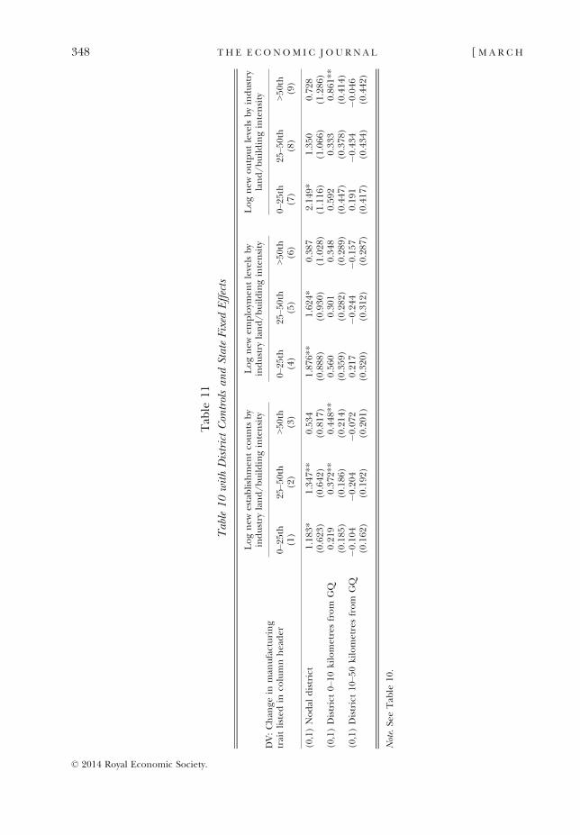
Tab

le11

Table10withDistrictControlsan

dStateFixedEffects

DV:Chan

gein

man

ufacturing

traitlisted

inco

lumnheader

Lognew

establishmen

tco

unts

by

industry


Lognew

employm

entlevelsby

industry


Lognew

outputlevelsbyindustry


0–25

th25

–50th

>50

th0–

25th

25–5

0th

>50

th0–

25th

25–5

0th

>50

th(1)

(2)

(3)

(4)

(5)

(6)

(7)

(8)

(9)

(0,1)Nodal

district

1.18

3*1.34

7**

0.53

41.87

6**

1.62

4*0.38

72.14

9*1.35

00.72

8(0.623

)(0.642

)(0.817

)(0.888

)(0.930

)(1.028

)(1.116

)(1.066

)(1.286

)(0,1)District0–

10kilometresfrom

GQ

0.21

90.37

2**

0.44

8**

0.56

00.30

10.34

80.59

20.33

30.86

1**

(0.185

)(0.186

)(0.214

)(0.359

)(0.282

)(0.289

)(0.447

)(0.378

)(0.414

)(0,1)District10

–50kilometresfrom

GQ

�0.104

�0.204

�0.072

0.21

7�0

.244

�0.157

0.19

1�0

.434

�0.046

(0.162

)(0.192

)(0.201

)(0.320

)(0.312

)(0.287

)(0.417

)(0.434

)(0.442

)

Note.Se

eTab

le10

.



estimation uses the long-differenced approach in specification (1). The 0–10 kilometresdistricts show a pronounced growth in entry by industries that are land and buildingintensive. Especially for young firm establishments and output, the adjustment is weakeramong plants with limited land and building intensities compared to the top half (thereare no important differences between the two quartiles in the top half). Remarkably, theopposite pattern is generally observed in the top row for nodal districts – where nodaldistricts are experiencing heightened entry of industries that are less land and buildingintensive after theGQupgrades – andno consistent patterns are observed for districts 10–50 kilometres from the GQ network. Table 11 shows a similar picture after includingdistrict controls and state fixed effects and Appendix Tables A9 and A10 show instead aweak or opposite relationship is evident with labour andmaterials intensity. Using capitalintensity to group industries not surprisingly gives similar results to land and buildingintensity. These patterns suggest that the GQ upgrades aided the efficient sorting ofindustries across locations along the network.

0.4

0.4

Employment Allocation, Proximity to GQ

Employment Allocation, Proximity to NS-EW

0.2

Output Allocation, Proximity to GQ Output Allocation, Proximity to NS-EW

0.40.2

0.6

0.6

Share of output within 0-200 km of GQ, 2000

Share of employment within0-200 km of GQ, 2000

Share of output within0-200 km of NS–EW, 2000

Share of employment within 0-200 km of NS–EW, 2000

0.6

0.8

0.8 0.8

1.0

1.0

–10

12

21

0C

hang

e in

Allo

cativ

e E

ffic

ienc

yC

hang

e in

Allo

cativ

e E

ffic

ienc

y

Cha

nge

in A

lloca

tive

Eff

icie

ncy

Cha

nge

in A

lloca

tive

Eff

icie

ncy

–1

21

0–1

–10

12

1.0

0.40.2 0.6 0.8 1.0

(a) (b)

(c) (d)

Fig. 3. Change in Allocative Efficiency for Indian Organised Sector Industries from 2000 to 2007/9Notes. Panels (a) and (c) plot the change in allocative efficiency for 55 industries from 2000 to2007/9 based upon the initial share of activity in those industries along the GQ network in 2000.A 200 kilometre radius is employed, and panel (a) considers employment and panel (c)considers output. Panels (b) and (d) plot comparable graphs based upon the proximity ofindustries to the NS–EW highway system.



3.7. Changes in Allocative Efficiency

Our final exercise takes up directly the allocative efficiency of the Indian economy. In avery influential paper, Hsieh and Klenow (2009) describe the degree to which Indiaand China have a misallocation of activity towards unproductive manufacturing plants.That is, India has too much employment in plants that have low efficiency and too littleemployment in plants with high efficiency levels. We evaluate whether the GQupgrades are connected with improvements in allocative efficiency for industries thatwere mostly located near the GQ network in 2000, compared to those that were mostlyoff the GQ network. The hypothesis is that allocative efficiency will improve most inindustries that were initially positioned around the GQ network. This could be due tointernal plant improvements in operations, increases in competition and the entry/exit of plants and adjustments in price distortions.

Quantifying improvements in allocative efficiency is quite different from the district-level empirics undertaken thus far as we must look at the industry’s productionstructure as a whole. We thus calculate for the 55 three-digit industries in themanufacturing sample a measure of their allocative efficiency in 1994, 2000 and 2007/9. This measure is calculated as the negative of the standard deviation of TFP across theplants in an industry. Thus, a reduction in the spread of TFP is taken as animprovement in allocative efficiency.24

Panel (a) of Figure 3 plots the change in allocative efficiency (larger numbers beingimprovements in unit standard deviations) from 2000 to 2007/9 for industries againstthe share of employment for the industry that was within 200 kilometres of the GQnetwork in 2000. There is an upward slope in this relationship, providing some broadconfirmation for the hypothesis. Panel (b) shows that this relationship is not evident interms of proximity to the NS–EW system. Panels (c) and (d) repeat these graphs usingthe share of output within 200 kilometres of the two highway systems. Industries thatwere in closer proximity to the GQ system in 2000 exhibit sharper improvements inallocative efficiency from 2000 to 2007/9.

Table 12 provides variants of these Figures. Panel (a) considers proximity to theGQ network, while panel (b) considers industrial proximity to the NS–EW network.Column headers indicate outcome variables. Column 1 continues with our baselineestimates of changes from 2000 to 2007/9 with the underlying TFP estimates using theSivadasan (2009) methodology. Column 2 instead substitutes a measure of growth inallocative efficiency that builds from a residual TFP calculation approach at the plantlevel. Column 3 considers the change in allocative efficiency across the earlier periodof 1994–2000, before the GQ upgrades began.

Eachentry in theTable is froma separate regressionwith the rowheaderdescribing themetric used to estimate proximity to the GQ network. The point estimates from these

24 Hsieh and Klenow (2009) calculate their TFP measures as revenue productivity (TFPR) and physicalproductivity (TFPQ). In their model, revenue productivity (the product of physical productivity and a firm’soutput price) should be equated across firms in the absence of distortions. Hsieh and Klenow (2009) use theextent that TFPR differs across plants as a metric of plant-level distortions. When TFPQ and TFPR are jointlylog normally distributed, there is a simple closed-form expression for aggregate TFP. In this case, the negativeeffect of distortions on aggregate TFP can be summarised by the variance of log TFPR. Intuitively, the extentof misallocation is worse when there is greater dispersion of marginal products. The standard deviationmeasure picks up this feature.



various techniques are reasonably similar, generally being larger for estimation thatconsiders employment or output proximity. The measures built upon total outputproximity or upon young firm activity in 2000 show the strongest statistical precision.They suggest that each 10% increase in the share of an industry’s activity near the GQnetwork in 2000 is associated with about a 0.07 unit standard deviation increase inallocative efficiency to 2007/9.

Column 3 does not find evidence of a link before 2000 and we find null resultsin panel (b)’s focus on proximity to the NS–EW network. These results are robustto controlling for the land and building intensity of an industry, calculatingproximity to the GQ network using a 50 kilometres range, and similar exercises.With 55 data points, there are natural limits on the extensions and robustnesschecks that can be undertaken but these exercises provide some confidence in theconclusion that the GQ upgrades had a positive impact for the allocative efficiencyof India’s manufacturing sector. This impact may have been particularly strong for

Table 12

Estimation of the Impact of GQ Improvements on Allocative Efficiency

Change in allocativeefficiency 2000–2007/9,

Sivadasan, L-P

Change in allocativeefficiency 2000–2007/9,

Residual

Change in allocativeefficiency 1994–2000,

Sivadasan, L-P(1) (2) (3)

(a) Share of industry activity within 200 kilometres of GQ, initial periodTotal plants 0.510 0.612 �0.295

(0.467) (0.450) (0.214)Total employment 0.718 0.796* �0.233

(0.436) (0.419) (0.210)Total output 0.710* 0.810** �0.242

(0.415) (0.398) (0.293)Young plants 0.319 0.380 �0.263

(0.351) (0.344) (0.172)Young employment 0.675** 0.792** �0.255**

(0.325) (0.313) (0.125)Young output 0.579** 0.668*** �0.275*

(0.255) (0.241) (0.149)

(b) Share of industry activity within 200 kilometres of NS–EW, initial period

Total plants 0.352 0.471 0.059(0.676) (0.654) (0.200)

Total employment �0.012 0.087 0.145(0.468) (0.462) (0.197)

Total output 0.248 0.270 0.001(0.519) (0.502) (0.210)

Young plants �0.042 �0.067 �0.063(0.391) (0.384) (0.231)

Young employment 0.068 0.040 0.106(0.282) (0.284) (0.178)

Young output 0.037 �0.013 0.126(0.239) (0.238) (0.150)

Notes. Each Table entry is from separate estimation. Estimation in columns 1 and 2 of panel (a) considers thechange in the allocative efficiency of organised-sector manufacturing from 2000 to 2007/9 by initialproximity to the GQ network in 2000. Column 3 presents a similar exercise from 1994 to 2000 during the pre-period before construction began. Panel (b) considers the placebo case of proximity to NS–EW system.Allocative efficiency is calculated using TFP estimates described in the column header. Regressors areexpressed in shares. Estimation reports robust standard errors, contains 55 observations and is unweighted.



industries where new activity was already occurring in a modest band around thenetwork.25

4. Discussion and Conclusions

This study finds that the GQ upgrades led to a substantial increase in manufacturingactivity. This growth included higher entry rates, incumbent productivity expansion,adjustments in the spatial sorting of industries and improved allocative efficiency in themanufacturing industries initially located along the GQ network. We close this articleby further discussing the economic magnitudes of the GQ reforms by the end of thesample period and what might lie ahead. These discussions, by their nature, requirestepping beyond the econometric analyses conducted, and the assumptions madebelow are important for the insights derived. We focus on output for this analysis. Theorganised sector accounts for over 80% of Indian manufacturing output and much ofthe work in this article points to a central connection of the GQ upgrades to outputgrowth.

We start with the impact of the upgrades for the 0–10 kilometres districts. Ourpreferred estimates of output impacts to the end of the sample period are the 0.43(0.16) and 0.37 (0.21) co-efficients in panels (b) and (c) of Table 2 respectively.These estimates are quite robust to specification checks, and they grow somewhat inmagnitude in the IV analyses. Taking a mid-point of 0.4 suggests a 49% overalloutput increase from initial values for the average district located near the GQnetwork. Compared to pre-period levels, this would be an increase of output levelsfor the average district from US$ 1.8 billion to US$ 2.6 billion. The actual increase,for reference, was to US$ 3.8 billion. The estimates would thus credit about 43% ofthe observed increase to the GQ upgrades, with the rest due to general expansionof Indian manufacturing and the accentuated development of manufacturing alongother dimensions that these districts possess (e.g. education levels).

Looking forward, it seems that the scope for further increase in output is relativelymodest. While panel (d) of Figure 2 shows sustained growth from 2006–9 in totaloutput levels, we expect this upward trend to flatten and stabilise for the long term.This forecast comes from consideration of the drivers of growth:

(i) continued new entry along the GQ network;(ii) the growth to scale of past entrants to these districts since the upgrades; and(ii) the growth of incumbents present from before 2000.

The second and third effects combine multiple elements – selection and exit amongfirms, output expansion among survivors and reallocation, and within-firm productivity

25 Unreported estimations suggest that increases in price competition may have played a role. Wegenerally find accentuated declines in output price dispersion over the 2000 to 2007/9 period for industrieslocated closer to the GQ network. As one example, every 10% increase in initial industry employment within200 kilometres of the GQ network is associated with a �0.14 (0.09) change in output price dispersion, withthe latter measured in unit standard deviations. These results, however, are not statistically significant and wedo not observe quality dispersions nor consumer prices by region. As such, we do not strongly emphasise thischannel but note suggestive evidence in this regard.



growth. Repeated cross-sectional data cannot perfectly separate these effects but we canprovide some informative calculations.

The first effect – the ongoing heightened rate of new output formation – appears tohave reached its long-term level. The dynamic estimation in panel (b) of Figure 2suggests that the increment of new entry over initial levels for districts along the GQnetwork stabilised by 2006–9. The heightened output formation at this time is 40% lessthan at its 2004 peak. Similarly, the share of establishments that are young firms isstable in these districts at 17–18% in 2007–9, after an increase from 14% in 2000. Thiseffect added about 11% output overall to the average district compared to initial levels.

The second driver – growth in scale of young cohorts of entrants – is often thoughtto be weak in the Indian context (Hsieh and Klenow, 2014). In this context, however,we observe some growth due to scaling in the 0–10 kilometres districts. Yet, there doesnot appear to be much scope for further growth in this regard either. The average sizeof all entrants since 2000 is 86% of all remaining pre-2000 incumbents by 2009; for themost recent cohort, the size ratio is 93%. Thus, while some further growth stimulusmay occur through growth of recent entrants, it seems unlikely from these conditionsthat such increments will be very large.

The third factor – growth of the surviving incumbents – is also unlikely to be a sourceof further growth. By 2009, this group accounts for about 68% of output in thesedistricts. While their output level increased, it has not kept pace with the district as awhole. This surviving group has been strongly selected during the 2000–9 period, so wedo not anticipate a mass exodus nor rapid growth for them.

Having reviewed these three components, we believe GQ’s output growth mayincrease beyond 49% but it is difficult to project it being much higher. Most of thelong-term impact of the GQ upgrades on the 0–10 kilometres districts appears to havebeen achieved. One uncertainty in this forecast is the role of entrants and reallocation.The data suggest stability is setting in on the rate of reallocations but it is possible thatreallocations could accelerate again in the future if some industries or plants face verylarge moving costs (e.g. recently built plants, agglomeration economies) that furtherweaken. Another source of uncertainty is how continued development of otherinfrastructure projects in India will cut into the connectivity advantage of districtsalong the GQ network (recall that the GQ upgrades were the first of seven phasesplanned).

With repeated cross-sectional data, we are not able to decompose the aggregategrowth gains precisely into the three channels described above. Some roughcalculations suggest a balance between entrants (the first two channels) andincumbents (the third channel). The 2009 output level of pre-2000 incumbents is148% of the district’s size in 2000 for the 0–10 kilometres districts; as a comparisonpoint, the similar ratio for the 50+ kilometres districts is 138%. These percentagesinclude initial levels and thus the net growth among pre-2000 incumbents is 48% and38% respectively. The 2009 output level of post-2000 entrants is 70% of the district’ssize in 2000 for the 0–10 kilometres districts, with the comparison point now being67%. Thus, in both distance bands, entrants account for a majority of net outputgrowth and the increment for the 0–10 kilometres districts is roughly comparable forboth incumbents and entrants, suggestive of mostly balanced growth roles thatsomewhat favour entrants.



With this long-term portrait, we can also make a cautious ballpark estimate of theoverall effect by considering the four spatial bands. We first make the importantassumption that the GQ upgrades had no effect on the 236 districts that are50 kilometres beyond the GQ network. This group, which accounted for 43% ofIndia’s output in the initial period, has served as a frequent control group and does notappear to be impacted substantially by the GQ network. Some evidence for thisassumption is found in the NS–EW placebo that compares distant districts from the GQnetwork by their proximity to the NS–EW network. Finding no major differences acrosssubgroups of districts in this analysis suggests that aggregate effects in the distantspatial range were unlikely to be material.

With this assumption in place, we next conclude from our analytical work that weakeffects accrued to districts 10–50 kilometres from the GQ network, which accountedfor a little under 10% of initial output levels. There may have been some declines, asevidenced by the small negative coefficients in Table 2, but these results are notstatistically significant. Even taking the point estimates as true values, the overallmagnitude would still be small (1–2% of total Indian manufacturing) given that thedeclines would be applied against a small share of the total manufacturing output inIndia.

The biggest growth comes from the 0 to 10 kilometres districts, which accounted for34% of initial levels. If long-term output development is modest from its current level,as argued above, we can use the 49% growth estimate. This would suggest a 17% outputgrowth contribution overall for India’s manufacturing sector.

Finally, we come to the question of the nodal districts, which represented 15% ofinitial output. Strictly speaking, the estimation would suggest that this group added afurther 9% output expansion. Some portion of this growth may be due to GQupgrades, but it is likely the case that a majority of the credit belongs elsewhere. Forrepresentative purposes, a value of 2% is assigned.

Thus, on a whole, our ballpark calculation would suggest that the GQ upgradesincreased manufacturing output by 15–19%. For reference, Indian manufacturingoutput doubled during this period and 37% of this growth occurred in the non-nodal0–10 kilometres districts along the GQ network. The estimates would thus creditsomething less than a fifth of the organised sector growth to better connectivityprovided by the enhanced GQ network, with all of that impact concentrated onadjacent districts. This calculation makes clear the key assumption underlying theanalysis – the only factors pushing forward these nearby districts, where the majority ofthis manufacturing growth occurred, were the GQ upgrades or the other traitsexplicitly modelled.26

These powerful effects may be localised to organised manufacturing. Khanna (2014)examines changes in night-time luminosity around the GQ upgrades. He findsevidence that the upgrades yielded weaker spatial differentials in terms of night-timelights, suggestive of a spreading out of economic development. There are sufficientoverlaps in our methodologies that the differences between the papers are not likely to

26 We do not attempt a full cost–benefit analysis given our uncertainty about the full costs of the upgrades.Using the initial cost estimates of the project and government reports that the project remained withinbudget, it is highly likely the benefits exceeded the costs.



be due to choices regarding empirical technique. Instead, it seems more likely that theorganised manufacturing sector reacted differently from other forms of economicactivity, and Section 2 noted the significantly weaker responses observed forunorganised manufacturing. Our findings thus point to a particular connection ofthe highway upgrades to the spatial development, sorting and allocative efficiency oflarge-scale manufacturing plants that ship inputs and outputs at a distance. Improve-ments in this sector’s efficiency and spatial organisation can generate substantialeconomic gains.

These outcomes are an important input into policy choices in India and otherdeveloping economies. This article provides quantitative estimates of the likelyeconomic growth associated with highway upgrades and the spatial impacts of theseinfrastructure projects. These estimates are most applicable to similar settings. Forexample, the GQ upgrades were the first phase of an overhaul to the inadequatetransport infrastructure of India. Thus, the impact may be larger than what would beobserved from marginal investments into more developed settings. Similarly, theprojects were undertaken during a period of economic growth, possibly allowing forgreater rates of entry and more adjustment in the location choice decisions of newentrants than in economies with stagnant growth (where infrastructure investment canalso be seen as a way to boost the economy). On the whole, our project speaks to thesevere constraints that inadequate infrastructure can have for the development ofmanufacturing in emerging economies and the potential growth that may follow fromalleviating that constraint.

World BankHarvard University, Bank of Finland, and NBER

Submitted: 3 November 2012Accepted: 28 July 2014

Additional Supporting Information may be found in the online version of this article:

Appendix A. Empirical Appendix.Data S1.

ReferencesAggarwal, S. (2013). ‘Do rural roads create pathways out of poverty? Evidence from India’, mimeo, Indian

School of Business.Ahluwalia, M. (2000). ‘Economic performance of states in the post reforms period’, Economic and Political

Weekly, vol. 35(19), pp. 1637–48.Ahsan, A. and Pages, C. (2008). ‘Are all labor regulations equal? Evidence from Indian manufacturing’,

Working Paper No. 3394, IZA.Aschauer, D.A. (1989). ‘Is public expenditure productive?’, Journal of Monetary Economics, vol. 23(2), pp. 177–

200.Banerjee, A., Duflo, E. and Qian, N. (2012). ‘On the road: access to transportation infrastructure and

economic growth in China’, Working Paper No. 17897, NBER.Baum-Snow, N. (2007). ‘Did highways cause suburbanization?’, Quarterly Journal of Economics, vol. 122(2),

pp. 775–805.Baum-Snow, N., Brandt, L., Henderson, V., Turner, M. and Zhang, Q. (2012). ‘Roads, railroads and

decentralization of Chinese cities’, mimeo, Brown University.



Baum-Snow, N. and Turner, M. (2013). ‘Transportation and the decentralization of Chinese cities’, mimeo,Brown University.

Besley, T. and Burgess, R. (2004). ‘Can labor regulation hinder economic performance? Evidence fromIndia’, Quarterly Journal of Economics, vol. 119(1), pp. 91–134.

Brown, D., Fay, M., Felkner, J., Lall, S. and Wang, H. (2008). ‘The death of distance? Economic implicationsof infrastructure improvement in Russia’, EIB Papers, vol. 13(2), pp. 126–47.

Chandra, A. and Thompson, E. (2000). ‘Does public infrastructure affect economic activity? Evidence fromthe rural interstate highway system’, Regional Science and Urban Economics, vol. 30(4), pp. 457–90.

Datta, S. (2011). ‘The impact of improved highways on Indian firms’, Journal of Development Economics, vol. 99(1), pp. 46–57.

Desmet, K., Ghani, E., O’Connell, S. and Rossi-Hansberg, E. (2012). ‘The spatial development of India’,Policy Research Paper No. 6060, World Bank.

Dinkelman, T. (2011). ‘The effects of rural electrification on employment: new evidence from South Africa’,American Economic Review , vol. 101(7), pp. 3078–108.

Donaldson, D. (2014). ‘Railroads of the Raj: estimating the impact of transportation infrastructure’, AmericanEconomic Review. (forthcoming)

Donaldson, D. and Hornbeck, R. (2012). ‘Railroads and American economic growth: new data and theory’,NBER Working Paper 19213.

Duflo, E. and Pande, R. (2007). ‘Dams’, Quarterly Journal of Economics, vol. 122(2), pp. 601–46.Duranton, G., Morrow, P. and Turner, M. (2014). ‘Roads and trade: evidence from the US’, Review of Economic

Studies, vol. 81(2), pp. 681–724.Duranton, G. and Puga, D. (2001). ‘Nursery cities: urban diversity, process innovation, and the life cycle of

products’, American Economic Review, vol. 91(5), pp. 1454–77.Duranton, G. and Puga, D. (2004). ‘Micro-foundations of urban agglomeration economies’, in (V.

Henderson and J.F. Thisse, eds.), Handbook of Regional and Urban Economics, Volume 4, pp. 2063–117,Amsterdam: North-Holland.

Duranton, G. and Turner, M. (2011). ‘The fundamental law of road congestion: evidence from US cities’,American Economic Review, vol. 101(6), pp. 2616–52.

Duranton, G. and Turner, M. (2012). ‘Urban growth and transportation’, Review of Economic Studies, vol. 79(4), pp. 1407–40.

Ellison, G., Glaeser, E. and Kerr, W. (2010). ‘What causes industry agglomeration? Evidence fromcoagglomeration patterns’, American Economic Review, vol. 100(3), pp. 1195–213.

Faber, B. (2014). ‘Trade integration, market size, and industrialization: evidence from China’s NationalTrunk Highway System’, Review of Economic Studies, vol. 81(3), pp. 1046–70.

Fernald, J.G. (1998). ‘Roads to prosperity? Assessing the link between public capital and productivity’,American Economic Review, vol. 89(3), pp. 619–38.

Fernandes, A. and Pakes, A. (2008). ‘Factor utilization in Indian manufacturing: a look at the World BankInvestment Climate Survey data’, Working Paper No. 14178, NBER.

Foster, L., Haltiwanger, J. and Syverson, C. (2008). ‘Reallocation, firm turnover and efficiency: selection onproductivity or profitability?’, American Economic Review, vol. 98(1), pp. 394–425.

Fretz, S. and Gorgas, C. (2013). ‘Regional economic effects of transport infrastructure expansions: evidencefrom the Swiss highway network’, Working Paper University of St Gallen, available athttp://www2.unine.ch/files/content/sites/irene/files/shared/documents/SSES/Fretz.pdf (last accessed: 6 December2014).

Ghani, E., Goswami, A. and Kerr, W. (2012). ‘Is India’s manufacturing sector moving away from cities?’,Working Paper No. 17992, NBER.

Ghani, E., Goswami, A. and Kerr, W. (2013). ‘The golden quadrilateral highway project and urban/ruralmanufacturing in India’, Working Paper No. 6620, World Bank.

Glaeser, E., Kerr, S. and Kerr, W. (2014). ‘Entrepreneurship and urban growth: an empirical assessment withhistorical mines’, Review of Economics and Statistics. (forthcoming)

Ghani, E., Kerr, W. and O’Connell, S. (2014). ‘Spatial determinants of entrepreneurship in India’, RegionalStudies, vol. 48(6), pp. 1071-89.

Gill, I. and Goh, C.-C. (2012). ‘Scale economies and cities’, World Bank Research Observer, vol. 25(2), pp. 235–62.

Gupta, P., Hasan, R. and Kumar, U. (2008). ‘What constrains Indian manufacturing?’, Working Paper No.211, ICRIER.

Gupta, P. and Kumar, U. (2010). ‘Performance of Indian manufacturing in the post reform period’, WorkingPaper, Munich Personal RePEc Archive (MPRA) Paper No. 24898.

Hasan, R. and Jandoc, K. (2010). ‘The distribution of firm size in India: what can survey data tell us?’,Working Paper No. 213, ADB Economics.

Henderson, V. (2010). ‘Cities and development’, Journal of Regional Science, vol. 50(1), pp. 515–40.Henderson, V., Lee, T., and Lee, Y.J. (2001). ‘Scale externalities in Korea’, Journal of Urban Economics, vol.

49(3), pp. 479–504.



Holl, A. (2013). ‘Highways and productivity in urban and rural locations’, Working Paper, Universitat deBarcelona-Institut d’Economia de Barcelona.

Holl, A. and Viladecans-Marsal, E. (2011). ‘Infrastructure and cities: the impact of new highways on urbangrowth’, Working Paper, Universitat de Barcelona-Institut d’Economia de Barcelona.

Hsieh, C. and Klenow, P. (2009). ‘Misallocation and manufacturing TFP in China and India’, Quarterly Journalof Economics, vol. 124(4), pp. 1403–48.

Hsieh, C. and Klenow, P. (2014). ‘The life cycle of plants in India and Mexico’, Quarterly Journal of Economics,vol. 129(3), pp. 1035–84.

Hsu, W.-T. and Zhang, H. (2011). ‘The fundamental law of highway congestion: evidence from Japaneseexpressways’, Working Paper, Chinese University of Hong Kong.

Kathuria, V., Natarajan, S., Raj, R. and Sen, K. (2010). ‘Organized versus Unorganized manufacturingperformance in India in the post-reform period’, Working Paper No. 20317, MPRA.

Khanna, G. (2014). ‘The road oft taken: highways to spatial development’, mimeo, University of Michigan,available at http://papers.ssrn.com/sol3/papers.cfm?abstract_id=2426835 (last accessed: 6 December2014).

Kochhar, K., Kumar, U., Rajan, R., Subramanian, A. and Tokatlidis, I.(2006). ‘India’s pattern of development:what happened, what follows?’, Working Paper No. 06/22, IMF.

Lahr, M., Duran, R. and Varughese, A. (2005). ‘Estimating the impact of highways on average travel velocitiesand market size’, mimeo, Center for Urban Policy Research, Rutgers University.

Levinsohn, J. and Petrin, A. (2003). ‘Estimating production functions using inputs to control forunobservables’, Review of Economic Studies, vol. 70(2), pp. 317–42.

McKinsey Global Institute. (2010). ‘India’s urban awakening: building inclusive cities, sustaining economicgrowth’, McKinsey & Company.

McKinsey Global Institute. (2012). ‘The shifting urban economic landscape: what does it mean for cities?’,McKinsey & Company.

Michaels, G. (2008). ‘The effect of trade on the demand for skill: evidence from the interstate highwaysystem’, Review of Economics and Statistics, vol. 90(4), pp. 683–701.

Mitra, A., Varoudakis, A. and V�eganzon�es, M. (1998). ‘State infrastructure and productive performance inIndian manufacturing’, Working Paper No. 139, OECD.

Munell, A. (1990). ‘Why has productivity growth declined? Productivity and public investment’, New EnglandEconomic Review, vol. January/February, pp. 3–22.

Nataraj, S. (2011). ‘The impact of trade liberalization on productivity: evidence from India’s formal andinformal manufacturing sectors’, Journal of International Economics, vol. 85(2), pp. 292–301.

Olley, S. and Pakes, A. (1996). ‘The dynamics of productivity in the telecommunications equipmentindustry’, Econometrica, vol. 64(6), pp. 1263–97.

Otto, G. and Voss, G. (1994). ‘Public capital and private sector productivity’, Economic Record, vol. 70(209), pp.121–32.

Qin, Y. (2014). ‘No county left behind? The distributional impact of high-speed rail upgrade in China’,Working Paper, Cornell University.

Roberts, M., Deichmann, U., Fingleton, B. and Shi, T. (2012). ‘Evaluating China’s road to prosperity: a neweconomic geography approach’, Regional Science and Urban Economics, vol. 42(4), pp. 580–94.

Rosenthal, S. and Strange, W. (2004). ‘Evidence on the nature and sources of agglomeration economies’, in(V. Henderson and J. F. Thisse, eds.), Handbook of Regional and Urban Economics, Volume 4, pp. 2119–71,Amsterdam: North-Holland.

Sivadasan, J. (2009). ‘Barriers to competition and productivity: evidence from India’, BE Journal of EconomicAnalysis & Policy, vol. 9(1), Article 42.

Subramanian, A. (2012a). ‘The ideas India must shed’, Real Time Economic Issues Watch, June 4th, 2012.Subramanian, A. (2012b). ‘What is India’s real growth potential’, Business Standard, May 23, 2012.The Economic Times. (2012). ‘Highway development requires Rs 200 cr investment every day’. April 29, 2012.Ulimwengu, J., Funes, J., Headey, D. and You, L. (2009). ‘Paving the way for development? The impact of

transport infrastructure on agricultural production and poverty reduction in the democratic republic ofCongo’, Discussion Paper No. 00944, IFPRI.

World Development Report. (2009). Reshaping Economic Geography, Washington, DC: The World Bank.World Road Statistics. (2009). World Road Statistics 2009: Data 2002–2007, Geneva: International Road

Federation.Xu, H. and Nakajima, K. (2013). ‘Highways and development in the peripheral regions of China’, Working

Paper, Institute of Economic Research Hitotsubashi University.



Documents

Highway to Success: The Impact of the Golden … Files/Ghani_Grover_Kerr... · HIGHWAY TO SUCCESS: THE IMPACT OF THE GOLDEN QUADRILATERAL PROJECT FOR THE LOCATION AND PERFORMANCE