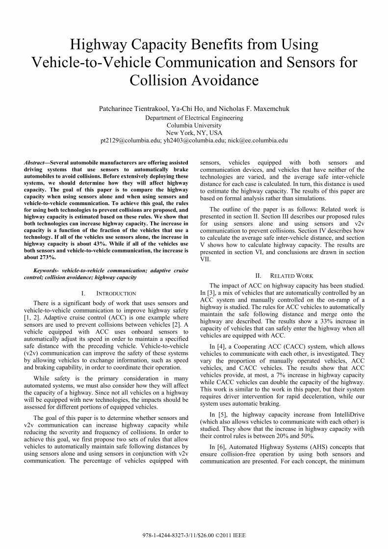
Highway Capacity Benefits from Using Vehicle-to-Vehicle Communication and Sensors for

Collision Avoidance

Patcharinee Tientrakool, Ya-Chi Ho, and Nicholas F. Maxemchuk Department of Electrical Engineering

Columbia University New York, NY, USA

pt2129@columbia.edu; yh2403@columbia.edu; nick@ee.columbia.edu

Abstract—Several automobile manufacturers are offering assisted driving systems that use sensors to automatically brake automobiles to avoid collisions. Before extensively deploying these systems, we should determine how they will affect highway capacity. The goal of this paper is to compare the highway capacity when using sensors alone and when using sensors and vehicle-to-vehicle communication. To achieve this goal, the rules for using both technologies to prevent collisions are proposed, and highway capacity is estimated based on these rules. We show that both technologies can increase highway capacity. The increase in capacity is a function of the fraction of the vehicles that use a technology. If all of the vehicles use sensors alone, the increase in highway capacity is about 43%. While if all of the vehicles use both sensors and vehicle-to-vehicle communication, the increase is about 273%.

Keywords- vehicle-to-vehicle communication; adaptive cruise control; collision avoidance; highway capacity

I. INTRODUCTION There is a significant body of work that uses sensors and

vehicle-to-vehicle communication to improve highway safety [1, 2]. Adaptive cruise control (ACC) is one example where sensors are used to prevent collisions between vehicles [2]. A vehicle equipped with ACC uses onboard sensors to automatically adjust its speed in order to maintain a specified safe distance with the preceding vehicle. Vehicle-to-vehicle (v2v) communication can improve the safety of these systems by allowing vehicles to exchange information, such as speed and braking capability, in order to coordinate their operation.

While safety is the primary consideration in many automated systems, we must also consider how they will affect the capacity of a highway. Since not all vehicles on a highway will be equipped with new technologies, the impacts should be assessed for different portions of equipped vehicles.

The goal of this paper is to determine whether sensors and v2v communication can increase highway capacity while reducing the severity and frequency of collisions. In order to achieve this goal, we first propose two sets of rules that allow vehicles to automatically maintain safe following distances by using sensors alone and using sensors in conjunction with v2v communication. The percentage of vehicles equipped with

sensors, vehicles equipped with both sensors and communication devices, and vehicles that have neither of the technologies are varied, and the average safe inter-vehicle distance for each case is calculated. In turn, this distance is used to estimate the highway capacity. The results of this paper are based on formal analysis rather than simulations.

The outline of the paper is as follows: Related work is presented in section II. Section III describes our proposed rules for using sensors alone and using sensors and v2v communication to prevent collisions. Section IV describes how to calculate the average safe inter-vehicle distance, and section V shows how to calculate highway capacity. The results are presented in section VI, and conclusions are drawn in section VII.

II. RELATED WORK The impact of ACC on highway capacity has been studied.

In [3], a mix of vehicles that are automatically controlled by an ACC system and manually controlled on the on-ramp of a highway is studied. The rules for ACC vehicles to automatically maintain the safe following distance and merge onto the highway are described. The results show a 33% increase in capacity of vehicles that can safely enter the highway when all vehicles are equipped with ACC.

In [4], a Cooperating ACC (CACC) system, which allows vehicles to communicate with each other, is investigated. They vary the proportion of manually operated vehicles, ACC vehicles, and CACC vehicles. The results show that ACC vehicles provide, at most, a 7% increase in highway capacity while CACC vehicles can double the capacity of the highway. This work is similar to the work in this paper, but their system requires driver intervention for rapid deceleration, while our system uses automatic braking.

In [5], the highway capacity increase from IntelliDrive (which also allows vehicles to communicate with each other) is studied. They show that the increase in highway capacity with their control rules is between 20% and 50%.

In [6], Automated Highway Systems (AHS) concepts that ensure collision-free operation by using both sensors and communication are presented. For each concept, the minimum

978-1-4244-8327-3/11/$26.00 ©2011 IEEE

safe inter-vehicle distance and maximum possible highway capacity is calculated. This paper is very similar to what we are doing; however, they use different rules to avoid collisions and pass different information about the operation of a vehicle. Furthermore, some AHS concepts require additional infrastructure along roads, while we use communications techniques that do not require additional infrastructure.

In our paper, vehicle-to-vehicle communication is based on our recently developed Reliable Neighborcast Protocol (RNP) [8]. RNP allows each vehicle to reliably communicate with all of its neighbors within a specified distance. This is different from the related work; which only allows vehicles to communicate with their immediate neighbors. Communicating with all of the vehicles in a neighborhood provides a faster response to a situation; which is similar to drivers who respond to situations that are several vehicles away rather than just observing the vehicle in front of them.

III. RULES FOR SENSORS AND V2V COMMUNICATION In this section, the different types of vehicles on a highway

are described in section A. Then the rules for using sensors alone and using sensors in conjunction with v2v communication are presented in sections B and C.

A. Types of Vehicles on a Highway There are three types of vehicles on a highway. 1) Manual Vehicles; which have neither sensors nor

communication and are manually controlled. 2) Vehicles with Sensors; which have onboard sensors but no

communication devices and are automatically controlled according to the rules in section B.

3) Communicating Vehicles; which have both sensors and communication devices and are automatically controlled according to the rules in section C.

B. Rules for Vehicles with Sensors

Figure 1. Variables related to the rules for vehicles with sensors.

Fig. 1 shows variables related to the rules for vehicles with sensors. All vehicles on a highway are assumed to move at the same speed, V km/h. Each vehicle has its own maximum deceleration rate (ao) in m/s2. Df is the safe following distance in meters that the vehicle with sensors maintains to the preceding vehicle.

Df is calculated by assuming that the maximum deceleration rates of vehicles are between a maximum deceleration rate amax and a minimum deceleration rate amin. In order to avoid collisions with the preceding vehicle, we assume the worst-case scenario; in which the preceding vehicle can decelerate at the maximum deceleration rate amax. We assume that we monitor and know our own deceleration rate ao, under the current road and load conditions. In our results, we use amin =-5 m/s2 and amax=-8.5 m/sec2, as in [7].

The vehicle with sensors always maintain Df, which is calculated from its perception-reaction time and the difference

in the deceleration rate between itself and the preceding vehicle:

Df =(Ts*V/3.6) +[V2/(25.92|ao|)]–[V2/(25.92|amax|)] (1) where Ts is the delay until a vehicle with sensors detects an

emergency situation (when its preceding vehicle suddenly brakes) and the brake is automatically applied. This delay includes the mechanical response time of an automobile braking system. The constant 3.6 is to convert vehicle speed V from km/h to m/s. The terms 25.92|a| are from 2|a| times 12.96, which is the constant to convert V2 from (km/h)2 to (m/s)2.

C. Rules for Communicating Vehicles Each communicating vehicle uses RNP [8] to communicate

with its neighboring vehicles. The delay bound until RNP reliably delivers a message from a vehicle to all its neighboring vehicles is Tp. It depends on the number of vehicles in a neighborhood and some other protocol parameters. The details for the performance RNP are in [8]. Vehicles that use RNP periodically exchange messages so that they know which of their neighbors can communicate.

Communicating vehicles use communications to exchange information on their deceleration rates and to provide a notification of an emergency stop. By exchanging information on deceleration rates, communicating vehicles do not have to assume the worst-case deceleration rates when calculating the safe following distance Df that they have to maintain to their preceding vehicles. Instead, the vehicles negotiate a group deceleration rate, ac, before an emergency stop. Communicating vehicles notify their neighbors when an emergency stop occurs by using RNP to transmit a warning message. By doing this, the time to detect a physical change in the operation of the preceding vehicle is reduced and a vehicle can respond to a stop by a vehicle several vehicles in front, as human drivers.

A communicating vehicle uses the negotiated deceleration rate, ac instead of its actual maximum deceleration rate, ao. The negotiated rate, ac, is the minimum deceleration rate among the group of neighboring communicating vehicles in the same lane without any vehicles with sensors or manual vehicles between them.

Fig. 2 shows an example of how communicating vehicles choose the deceleration rates to be used. Vehicles labeled with C are communicating vehicles; while vehicles labeled with M are manual vehicles or vehicles with sensors. Because of the three intervening manual or sensor vehicles v3, v5, v9, communicating vehicles v1 and v2 use the same negotiated deceleration rate -x, v4 uses its actual deceleration rate a4, and v6, v7, v8 use the same negotiated deceleration rate -y.

Figure 2. Negotiated deceleration rates used by communicating vehicles.

Similar to the sensor case, each communicating vehicle maintains the safe following distance Df to its preceding vehicle. However, the calculation of Df depends on whether or not its nearby vehicles can communicate as follows.

Case1: Neither the preceding nor following vehicle can communicate

In this case, the communicating vehicle has to rely on the information from its sensors. The vehicle uses its actual maximum deceleration rate ao in this case because both the vehicle in front of it and the vehicle behind it are not communicating vehicles. Therefore, the calculation for Df in this case is exactly the same as the one in section B.

Df =(Ts*V/3.6) +[V2/(25.92|ao|)]–[V2/(25.92|amax|)] (2)

Case 2: The preceding vehicle cannot communicate, but the following vehicle can

In this case, the communicating vehicle also has to rely on its sensors. However, it will use the negotiated deceleration rate ac instead of the actual rate ao because the following vehicle is also a communicating vehicle. So,

Df = (Ts*V/3.6) +[V2/(25.92|ac|)]–[V2/(25.92|amax|)] (3)

Case 3: The preceding vehicle can communicate In this case, the communicating vehicle and its preceding

vehicle agree to use the same negotiated rate ac and the communicating vehicle can detect an emergency situation within Tp second after the preceding vehicle uses RNP to transmit a warning message. The perception-reaction time of a communicating vehicle (Tc) is the sum of the delay until it detects the situation (Tp) and the delay until the brake is automatically applied. Therefore,

Df = Tc*V/3.6 (4)

IV. AVERAGE SAFE INTER-VEHICLE DISTANCE CALCULATION

This section shows how to calculate the average safe inter-vehicle distance that ensures no collisions with preceding vehicles. Each vehicle needs to maintain different safe following distances depending on the types of itself, its preceding vehicle, and its following vehicle. Therefore, the percentage of each type of vehicle on a highway affects the average safe inter-vehicle distance. In this section, we first present the equation for calculating the average safe inter-vehicle distance ( ), followed by the details on how to calculate the average safe following distance that each vehicle has to maintain in different cases.

The average safe inter-vehicle distance is calculated as:

= (Pm*Dm) + (Ps*Ds) + (Pc*Dc) (5) Pm, Ps, and Pc are the probability that a vehicle is a manual

vehicle, a vehicle with sensors, and a communicating vehicle respectively, where Pm+ Ps + Pc = 1. Dm, Ds, and Dc are the average safe following distance that manual vehicles, vehicles with sensors, and communicating vehicles maintain to their preceding vehicles respectively.

The average safe following distances Dm, Ds, and Dc are calculated as follows.

1. Dm calculation According to [4], the time gaps that manual drivers maintain

with their preceding vehicles are assumed to be normally distributed with a mean of 1.1 second and standard deviation of

0.15 second. This value was taken from a statistical analysis of the UMTRI ACC FOT baseline case human driving data. We will assume that a time gap of 1.1 second is safe and adequate for manual drivers to stop their vehicles without colliding with the preceding vehicles. So, the average safe following distance for manual vehicles is:

Dm = 1.1*V/3.6 (6)

2. Ds calculation A vehicle with sensors uses (1) in the rules in section III(B)

to calculate the safe following distance that it has to maintain. Assuming that the maximum deceleration rate ao of a vehicle is uniformly distributed over the interval [amax, amin], the average safe following distance that vehicles with sensors maintain is:

Ds= (Ts*V/3.6) + {V2 *ln(|amax|/|amin|) /[25.92* (|amax|–|amin|)]} – [V2/(25.92|amax|)] (7)

3. Dc calculation A communicating vehicle maintains different safe following

distances in 3 different cases according to the rules described in section III(C). Therefore, the average safe following distance that communicating vehicles maintain is

Dc = (P1*Dc1) + (P2*Dc2) + (P3*Dc3) (8) where P1, P2, and P3 are the probability that case 1, 2, and 3

occur respectively. Dc1, Dc2, and Dc3 are the average safe following distance that communicating vehicles maintain in case 1, 2, and 3 respectively. The probability and the average safe following distance for each case are calculated as follows.

Case1: Neither the preceding nor following vehicle can communicate

The probability that case 1 occurs is P1 = (Pm+Ps)2. In this case, the communicating vehicle maintains the same safe following distance as a vehicle with sensors does. Therefore,

Dc1 = Ds = (Ts*V/3.6) + {V2 *ln(|amax|/|amin|) /[25.92* (|amax| –|amin|)]} – [V2/(25.92|amax|)] (9)

Case 2: The preceding vehicle cannot communicate, but the following vehicle can

The probability that case 2 occurs is P2 = (Pm+Ps)*Pc. In this case, the communicating vehicle uses (3) to calculate the safe following distance. Therefore,

Dc2=(Ts*V/3.6) + – [V2/(25.92|amax|)]

= (Ts*V/3.6) – [V2/(25.92|amax|)]

+ (10)

where X is the absolute value of the negotiated deceleration rate that the communicating vehicle we are considering chooses to use, f(x) is the probability density function of X, and n is the average number of communicating vehicles (including the vehicle we are considering) that agree to use the same negotiated rate as the vehicle we are considering.

The negotiated deceleration rate depends on the number of communicating vehicles in a row behind the vehicle we are

considering and the actual deceleration rates of these communicating vehicles. If F(x) is the cumulative distribution

function of X, F(x) = 1 – P (the vehicle we are considering and all n-1

communicating vehicles in a row behind it have |actual maximum deceleration rate| > x)

F(x) =

(11)

In our case, the vehicle we are considering and the following vehicle are communicating vehicles; therefore, n is calculated as follows.

(12) If Pc < 1, then n = (2-Pc)/(1-Pc) and Dc2 is as shown in (10).

On the other hand, if Pc = 1, then n = ∞ and ac is equal to amin. So, Dc2 = (Ts*V/3.6)+[V2/(25.92|amin|)]–[V2/(25.92|amax|)].

Case 3: The preceding vehicle can communicate The probability that case 3 occurs is P3 = Pc. In this case, the

communicating vehicle uses (4) to calculate the safe following distance. Therefore,

Dc3 = Tc*V/3.6 (13)

(9)-(13) can be used to calculate Dc, then the average safe inter-vehicle distance can be calculated from Dm, Ds, and Dc as shown in (5).

V. HIGHWAY CAPACITY CALCULATION Reference [9] defines the capacity of a facility as the

maximum hourly rate at which persons or vehicles reasonably can be expected to traverse a point or a uniform section of a lane or roadway during a given time period under prevailing roadway, traffic, and control conditions. From this definition, highway capacity (C) in vehicles/hour/lane can be estimated as

C = 3600*V /[3.6*( l + )] = 1000*V/( l + ) (14)

where l is the average vehicle length in meters and is the average safe inter-vehicle distance calculated in section IV.

VI. RESULTS This section shows the average safe inter-vehicle distance

and highway capacity for three cases. In the first case, the percentage of each of the three types of vehicle is varied, but the speed of vehicles (V) is fixed at 100 km/h. The second case is the same as the first case except that there are only two types of vehicle on a highway i.e. manual vehicles and communicating vehicles, or manual vehicles and vehicles with sensors. In the third case, the vehicle speeds are varied from 0 to 120 km/h, but there is only one type of vehicle on a highway.

The following assumptions are used in all cases. All vehicles move with the same speed. amin and amax are -5 m/s2 and -8.5 m/s2 respectively [7]. Manual drivers maintain the average time gap of 1.1 s as in [4], Ts is 0.245 s as in [3], and Tc is 0.181 s. Tc is the sum of the delay Tp from RNP and the delay until the brake is applied. Tp is 0.081 s; which is the delay bound that RNP

provides message delivery to all neighboring vehicles within 125 m of a sending vehicle assuming that the average vehicle length (l) is 4.3 m as in [10]. The brake delay is 0.1 s as in [11].

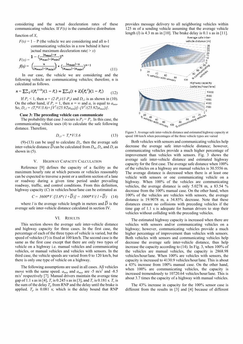
Figure 3. Average safe inter-vehicle distance and estimated highway capacity at speed 100 km/h when percentages of the three vehicle types are varied

Both vehicles with sensors and communicating vehicles help decrease the average safe inter-vehicle distance; however, communicating vehicles provide a much higher percentage of improvement than vehicles with sensors. Fig. 3 shows the average safe inter-vehicle distance and estimated highway capacity for the first case. The average safe distance when 100% of the vehicles on a highway are manual vehicles is 30.5556 m. The average distance is decreased when there is at least one vehicle with sensors or one communicating vehicle on a highway. When 100% of the vehicles are communicating vehicles, the average distance is only 5.0278 m, a 83.54 % decrease from the 100% manual case. On the other hand, when 100% of the vehicles are vehicles with sensors, the average distance is 19.9078 m, a 34.85% decrease. Note that these distances ensure no collisions with preceding vehicles if the time gap of 1.1 s is adequate for human drivers to stop their vehicles without colliding with the preceding vehicles.

The estimated highway capacity is increased when there are vehicles with sensors and/or communicating vehicles on a highway; however, communicating vehicles provide a much higher percentage of improvement than vehicles with sensors. Both vehicles with sensors and communicating vehicles help decrease the average safe inter-vehicle distance, thus help increase the capacity according to (14). In Fig. 3, when 100% of the vehicles are manual vehicles, the capacity is 2868.98 vehicles/hour/lane. When 100% are vehicles with sensors, the capacity is increased to 4130.9 vehicles/hour/lane. This is about a 43% increase from 100% manual case. On the other hand, when 100% are communicating vehicles, the capacity is increased tremendously to 10720.64 vehicles/hour/lane. This is about 3.7 times the capacity of a highway with manual vehicles.

The 43% increase in capacity for the 100% sensor case is different from the results in [3] and [4] because of different

assumptions and ways of using sensors. [3] assumes that the expected speed of vehicles with sensors and manual vehicles are 120 and 110 km/h respectively and focuses on the on-ramp traffic merging onto a highway. [4] requires the vehicles with sensors to maintain a fixed large time gap of 1.4 s from the preceding vehicles to allow their drivers to intervene in emergency situations, so their percentage increase in capacity is smaller than ours.

In the case of 100% communicating vehicles, our results show a much higher percentage increase in capacity than [4] and [5]. This is due to the small message delivery delay provided by RNP; which results in Tc of only 0.181 s. In addition, since all vehicles choose to use the same deceleration rate in this case, we do not need the part of the safe distance due to the difference in the deceleration rates.

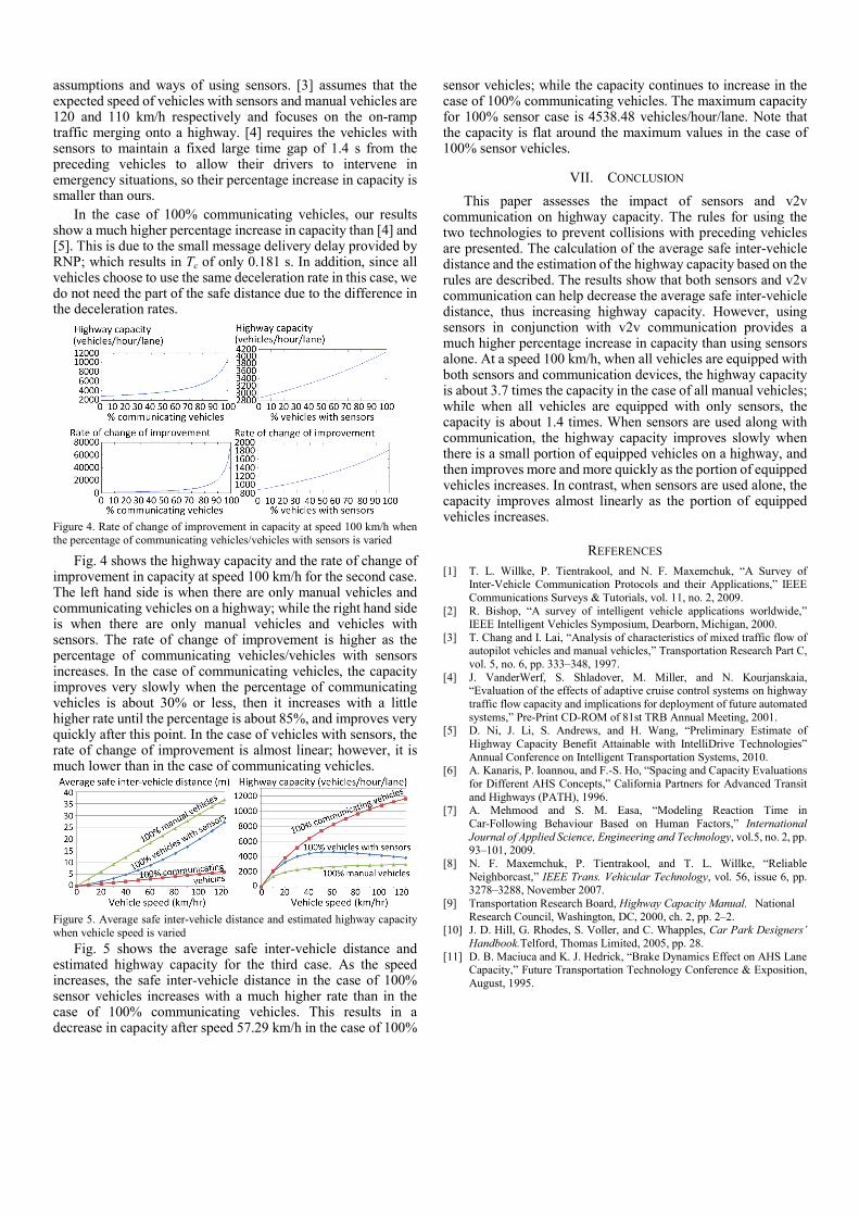
Figure 4. Rate of change of improvement in capacity at speed 100 km/h when the percentage of communicating vehicles/vehicles with sensors is varied

Fig. 4 shows the highway capacity and the rate of change of improvement in capacity at speed 100 km/h for the second case. The left hand side is when there are only manual vehicles and communicating vehicles on a highway; while the right hand side is when there are only manual vehicles and vehicles with sensors. The rate of change of improvement is higher as the percentage of communicating vehicles/vehicles with sensors increases. In the case of communicating vehicles, the capacity improves very slowly when the percentage of communicating vehicles is about 30% or less, then it increases with a little higher rate until the percentage is about 85%, and improves very quickly after this point. In the case of vehicles with sensors, the rate of change of improvement is almost linear; however, it is much lower than in the case of communicating vehicles.

Figure 5. Average safe inter-vehicle distance and estimated highway capacity when vehicle speed is varied

Fig. 5 shows the average safe inter-vehicle distance and estimated highway capacity for the third case. As the speed increases, the safe inter-vehicle distance in the case of 100% sensor vehicles increases with a much higher rate than in the case of 100% communicating vehicles. This results in a decrease in capacity after speed 57.29 km/h in the case of 100%

sensor vehicles; while the capacity continues to increase in the case of 100% communicating vehicles. The maximum capacity for 100% sensor case is 4538.48 vehicles/hour/lane. Note that the capacity is flat around the maximum values in the case of 100% sensor vehicles.

VII. CONCLUSION This paper assesses the impact of sensors and v2v

communication on highway capacity. The rules for using the two technologies to prevent collisions with preceding vehicles are presented. The calculation of the average safe inter-vehicle distance and the estimation of the highway capacity based on the rules are described. The results show that both sensors and v2v communication can help decrease the average safe inter-vehicle distance, thus increasing highway capacity. However, using sensors in conjunction with v2v communication provides a much higher percentage increase in capacity than using sensors alone. At a speed 100 km/h, when all vehicles are equipped with both sensors and communication devices, the highway capacity is about 3.7 times the capacity in the case of all manual vehicles; while when all vehicles are equipped with only sensors, the capacity is about 1.4 times. When sensors are used along with communication, the highway capacity improves slowly when there is a small portion of equipped vehicles on a highway, and then improves more and more quickly as the portion of equipped vehicles increases. In contrast, when sensors are used alone, the capacity improves almost linearly as the portion of equipped vehicles increases.

REFERENCES [1] T. L. Willke, P. Tientrakool, and N. F. Maxemchuk, “A Survey of

Inter-Vehicle Communication Protocols and their Applications,” IEEE Communications Surveys & Tutorials, vol. 11, no. 2, 2009.

[2] R. Bishop, “A survey of intelligent vehicle applications worldwide,” IEEE Intelligent Vehicles Symposium, Dearborn, Michigan, 2000.

[3] T. Chang and I. Lai, “Analysis of characteristics of mixed traffic flow of autopilot vehicles and manual vehicles,” Transportation Research Part C, vol. 5, no. 6, pp. 333–348, 1997.

[4] J. VanderWerf, S. Shladover, M. Miller, and N. Kourjanskaia, “Evaluation of the effects of adaptive cruise control systems on highway traffic flow capacity and implications for deployment of future automated systems,” Pre-Print CD-ROM of 81st TRB Annual Meeting, 2001.

[5] D. Ni, J. Li, S. Andrews, and H. Wang, “Preliminary Estimate of Highway Capacity Benefit Attainable with IntelliDrive Technologies” Annual Conference on Intelligent Transportation Systems, 2010.

[6] A. Kanaris, P. Ioannou, and F.-S. Ho, “Spacing and Capacity Evaluations for Different AHS Concepts,” California Partners for Advanced Transit and Highways (PATH), 1996.

[7] A. Mehmood and S. M. Easa, “Modeling Reaction Time in Car-Following Behaviour Based on Human Factors,” International Journal of Applied Science, Engineering and Technology, vol.5, no. 2, pp. 93–101, 2009.

[8] N. F. Maxemchuk, P. Tientrakool, and T. L. Willke, “Reliable Neighborcast,” IEEE Trans. Vehicular Technology, vol. 56, issue 6, pp. 3278–3288, November 2007.

[9] Transportation Research Board, Highway Capacity Manual. National Research Council, Washington, DC, 2000, ch. 2, pp. 2–2.

[10] J. D. Hill, G. Rhodes, S. Voller, and C. Whapples, Car Park Designers’ Handbook.Telford, Thomas Limited, 2005, pp. 28.

[11] D. B. Maciuca and K. J. Hedrick, “Brake Dynamics Effect on AHS Lane Capacity,” Future Transportation Technology Conference & Exposition, August, 1995.