Embed Size (px)
Citation preview

I Bryson. Amendments by E Maxwell, M Doran, E Traynor & C Cassells Page 1 of 107
Paisley Grammar School Mathematics Department
Higher Mathematics
Notes
2017/18
http://www.pgsmaths.co.uk
I Bryson. Amendments by E Maxwell, M Doran, E Traynor & C Cassells Page 2 of 107
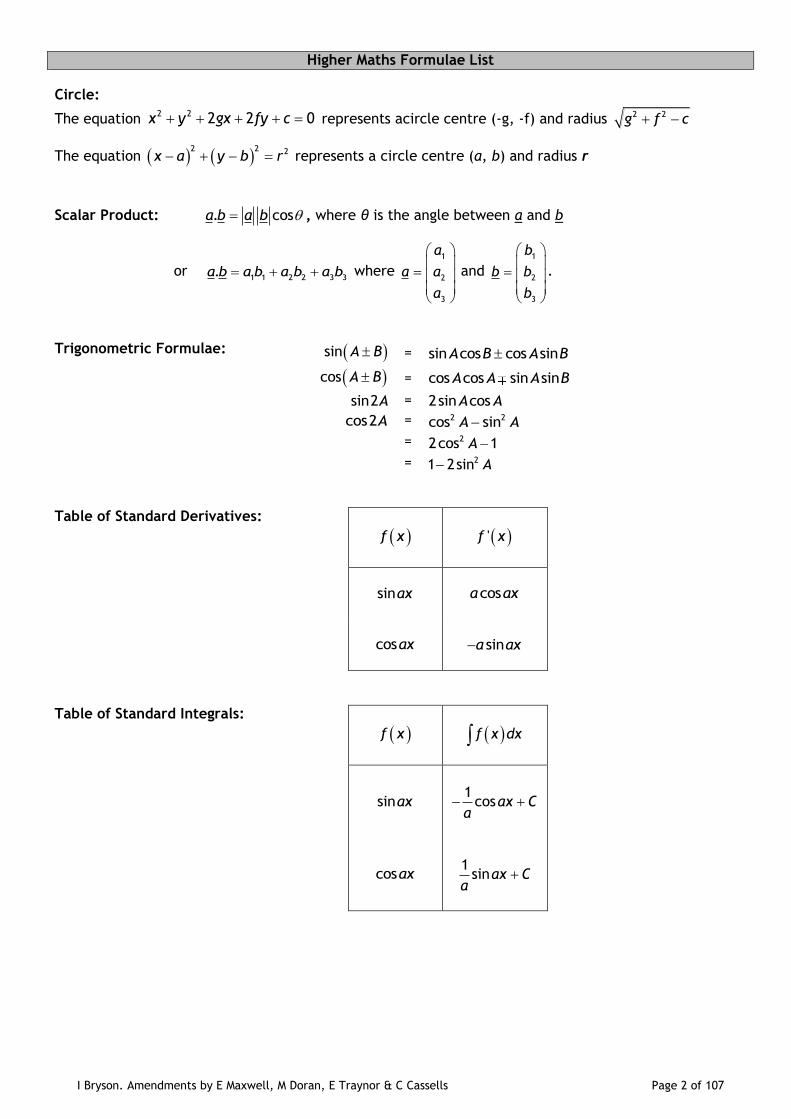
Higher Maths Formulae List
Circle:
The equation 2 2 2 2 0x y gx fy c represents acircle centre (-g, -f) and radius 2 2g f c
The equation 2 2 2x a y b r represents a circle centre (a, b) and radius r
Scalar Product: . cosa b a b , where θ is the angle between a and b
or 1 1 2 2 3 3
.a b a b a b a b where 1
2
3
a
a a
a
and 1
2
3
b
b b
b
.
Trigonometric Formulae: sin A B = sin cos cos sinA B A B
cos A B = cos cos sin sinA A A B
sin2A = 2sin cosA A cos2A = 2 2cos sinA A = 22cos 1A = 21 2sin A
Table of Standard Derivatives:
f x
'f x
sinax
cosa ax
cosax
sina ax
Table of Standard Integrals:
f x
f x dx
sinax
1cosax C
a
cosax
1sinax C
a
I Bryson. Amendments by E Maxwell, M Doran, E Traynor & C Cassells Page 3 of 107
The Straight Line
Revision from National 5
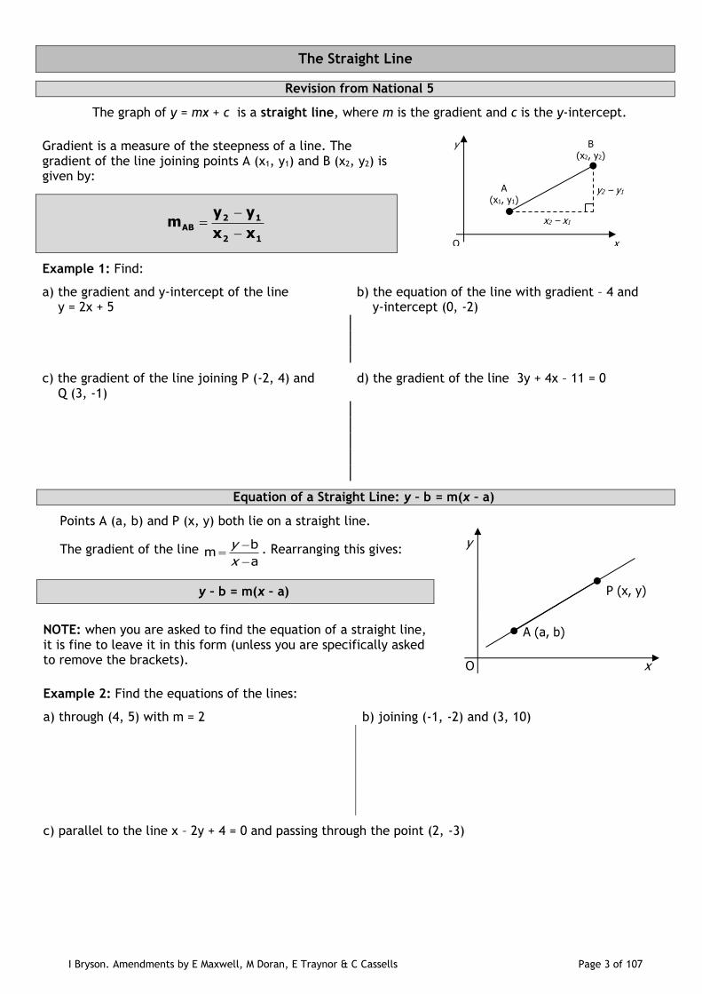
The graph of y = mx + c is a straight line, where m is the gradient and c is the y-intercept.
Gradient is a measure of the steepness of a line. The gradient of the line joining points A (x1, y1) and B (x2, y2) is given by:
12
12AB
xx
yym
Example 1: Find:
a) the gradient and y-intercept of the line y = 2x + 5
b) the equation of the line with gradient – 4 and y-intercept (0, -2)
c) the gradient of the line joining P (-2, 4) and Q (3, -1)
d) the gradient of the line 3y + 4x – 11 = 0
Equation of a Straight Line: y – b = m(x – a)
Points A (a, b) and P (x, y) both lie on a straight line.
The gradient of the line a
bm
x
y . Rearranging this gives:
y – b = m(x – a)
NOTE: when you are asked to find the equation of a straight line, it is fine to leave it in this form (unless you are specifically asked to remove the brackets).
Example 2: Find the equations of the lines:
a) through (4, 5) with m = 2 b) joining (-1, -2) and (3, 10)
c) parallel to the line x – 2y + 4 = 0 and passing through the point (2, -3)
x
y2 – y1
y
O
A (x1, y1)
x2 – x1
B (x2, y2)
A (a, b)
P (x, y)
x
y
O

I Bryson. Amendments by E Maxwell, M Doran, E Traynor & C Cassells Page 4 of 107
Equation of a Straight Line
y = mx + c AND Ax + By + C = 0
Example 3: Find the equation of the line through
(-5, -1) with m = 3
2 , giving your answer in the
form Ax + By + C = 0.
Example 4: Sketch the line 5x – 2y – 24 = 0 by finding the points where it crosses the x – and y – axes.
The Angle with the x-axis
The gradient of a line can also be described as the angle it makes with the positive direction of the x –axis.
As the y-difference is OPPOSITE the angle and the x-difference is ADJACENT to it, we get:
θtanmAB
(where θ is measured CLOCKWISE from the x-axis)
Example 5: Find the angle made with the positive direction of the x -axis and the lines:
a) y = x – 1 b) y = 5 – 3x c) joining the points (3, -2) and (7, 4)
Gradients of straight lines can be summarised as follows:
a) lines sloping up from left to right have positive gradients and make acute angles with the positive direction of the x-axis
b) lines sloping down from left to right have negative gradients and make obtuse angles with the positive direction of the x-axis
c) lines with equal gradients are parallel d) horizontal lines (parallel to the x -axis) have gradient zero and equation y = a e) vertical lines (parallel to the y -axis) have gradient undefined and equation x = b
A (x1, y1)
B (x2, y2)
x
y
O
y2 – y1
x2 – x1
θ
θ
●
●

I Bryson. Amendments by E Maxwell, M Doran, E Traynor & C Cassells Page 5 of 107
Collinearity
If three (or more) points lie on the same line, they are said to be collinear.
Example 6: Prove that the points D (-1, 5), E (0, 2) and F (4, -10) are collinear.
Perpendicular Lines
If two lines are perpendicular to each other (i.e. they meet at 90°), then: m1m2 = -1
Example 7: Show whether these pairs of lines are perpendicular:
a) x + y + 5 = 0 x – y – 7 = 0
b) 2x – 3y = 5 3x = 2y + 9
c) y = 2x - 5 6y = 10 – 3x
When asked to find the gradient of a line perpendicular to another, follow these steps:
1. Find the gradient of the given line 2. Flip it upside down 3. Change the sign (e.g. negative to positive)
Example 8: Find the gradients of the lines perpendicular to:
a) the line y = 3x - 12 b) a line with gradient = -1.5 c) the line 2y + 5x = 0
Example 9: Line L has equation x + 4y + 2 = 0. Find the equation of the line perpendicular to L which passes through the point (-2, 5).
I Bryson. Amendments by E Maxwell, M Doran, E Traynor & C Cassells Page 6 of 107
Midpoints and Perpendicular Bisectors
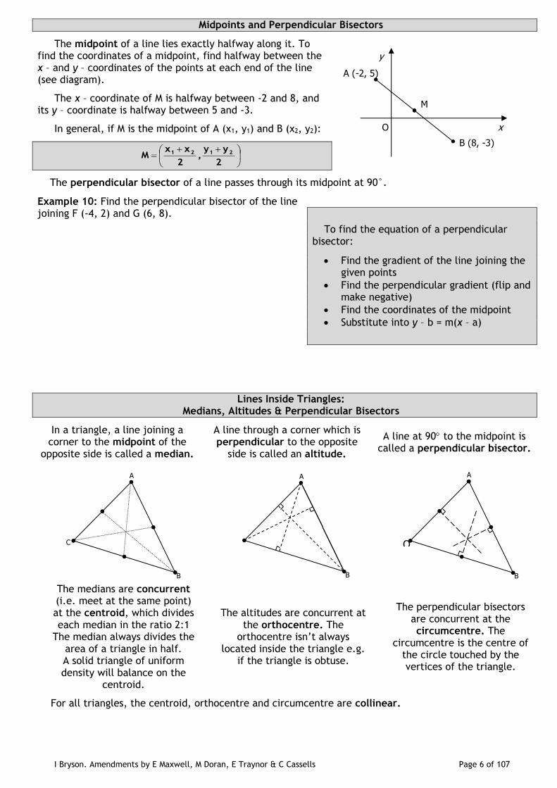
The midpoint of a line lies exactly halfway along it. To find the coordinates of a midpoint, find halfway between the x – and y – coordinates of the points at each end of the line (see diagram).
The x – coordinate of M is halfway between -2 and 8, and its y – coordinate is halfway between 5 and -3.
In general, if M is the midpoint of A (x1, y1) and B (x2, y2):
2
yy,
2
xxM 2121
The perpendicular bisector of a line passes through its midpoint at 90°.
Example 10: Find the perpendicular bisector of the line joining F (-4, 2) and G (6, 8).
To find the equation of a perpendicular bisector:
Find the gradient of the line joining the given points
Find the perpendicular gradient (flip and make negative)
Find the coordinates of the midpoint
Substitute into y – b = m(x – a)
Lines Inside Triangles: Medians, Altitudes & Perpendicular Bisectors
In a triangle, a line joining a corner to the midpoint of the
opposite side is called a median.
A line through a corner which is perpendicular to the opposite
side is called an altitude.
A line at 90 to the midpoint is called a perpendicular bisector.
The medians are concurrent (i.e. meet at the same point) at the centroid, which divides each median in the ratio 2:1
The median always divides the area of a triangle in half. A solid triangle of uniform density will balance on the
centroid.
The altitudes are concurrent at the orthocentre. The
orthocentre isn’t always located inside the triangle e.g.
if the triangle is obtuse.
The perpendicular bisectors are concurrent at the circumcentre. The
circumcentre is the centre of the circle touched by the vertices of the triangle.
For all triangles, the centroid, orthocentre and circumcentre are collinear.
A (-2, 5)
B (8, -3)
M
x
y
O
A
B
C
A
B
A
B
O
I Bryson. Amendments by E Maxwell, M Doran, E Traynor & C Cassells Page 7 of 107
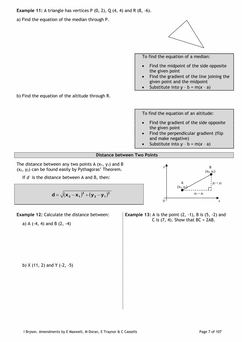
Example 11: A triangle has vertices P (0, 2), Q (4, 4) and R (8, -6).
a) Find the equation of the median through P.
To find the equation of a median:
Find the midpoint of the side opposite the given point
Find the gradient of the line joining the given point and the midpoint
Substitute into y – b = m(x – a)
b) Find the equation of the altitude through R.
To find the equation of an altitude:
Find the gradient of the side opposite the given point
Find the perpendicular gradient (flip and make negative)
Substitute into y – b = m(x – a)
Distance between Two Points
The distance between any two points A (x1, y1) and B (x2, y2) can be found easily by Pythagoras’ Theorem.
If d is the distance between A and B, then:
212
2
12 yyxxd
Example 12: Calculate the distance between: Example 13: A is the point (2, -1), B is (5, -2) and C is (7, 4). Show that BC = 2AB.
a) A (-4, 4) and B (2, -4) b) X (11, 2) and Y (-2, -5)
x
y2 – y1
y
O
A (x1, y1)
x2 – x1
B
(x2, y2)
I Bryson. Amendments by E Maxwell, M Doran, E Traynor & C Cassells Page 8 of 107
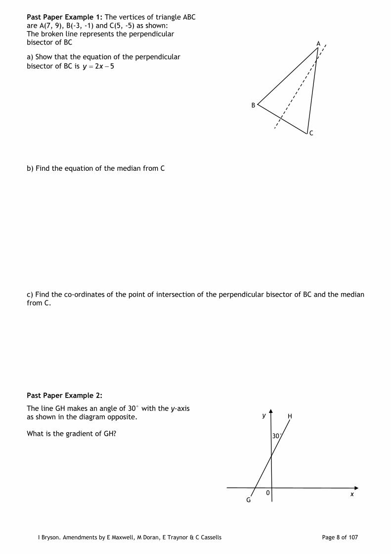
Past Paper Example 1: The vertices of triangle ABC are A(7, 9), B(-3, -1) and C(5, -5) as shown: The broken line represents the perpendicular bisector of BC
a) Show that the equation of the perpendicular
bisector of BC is 2 5y x
b) Find the equation of the median from C
c) Find the co-ordinates of the point of intersection of the perpendicular bisector of BC and the median from C.
Past Paper Example 2:
The line GH makes an angle of 30° with the y-axis as shown in the diagram opposite. What is the gradient of GH?
B
C
A
H y
x 0 G
30°
I Bryson. Amendments by E Maxwell, M Doran, E Traynor & C Cassells Page 9 of 107
Sets and Functions
A set is a group of numbers which share common properties. Some common sets are:
Natural Numbers N = {1, 2, 3, 4, 5,……}
Whole Numbers W = {0, 1, 2, 3, 4, 5,…..}
Integers Z = {…..,-3, -2, -1, 0, 1, 2, 3,…..}
Rational Numbers Q = all integers and fractions of them (e.g. ¾, -⅝, etc)
Real Numbers R = all rational and irrational numbers (e.g. etc.,,2 )
Sets are written inside curly brackets. The set with no members “{ }” is called the empty set.
means “is a member of”, e.g. 5 {3, 4, 5, 6, 7} means “is not a member of”, e.g. 5 {6, 7, 8}
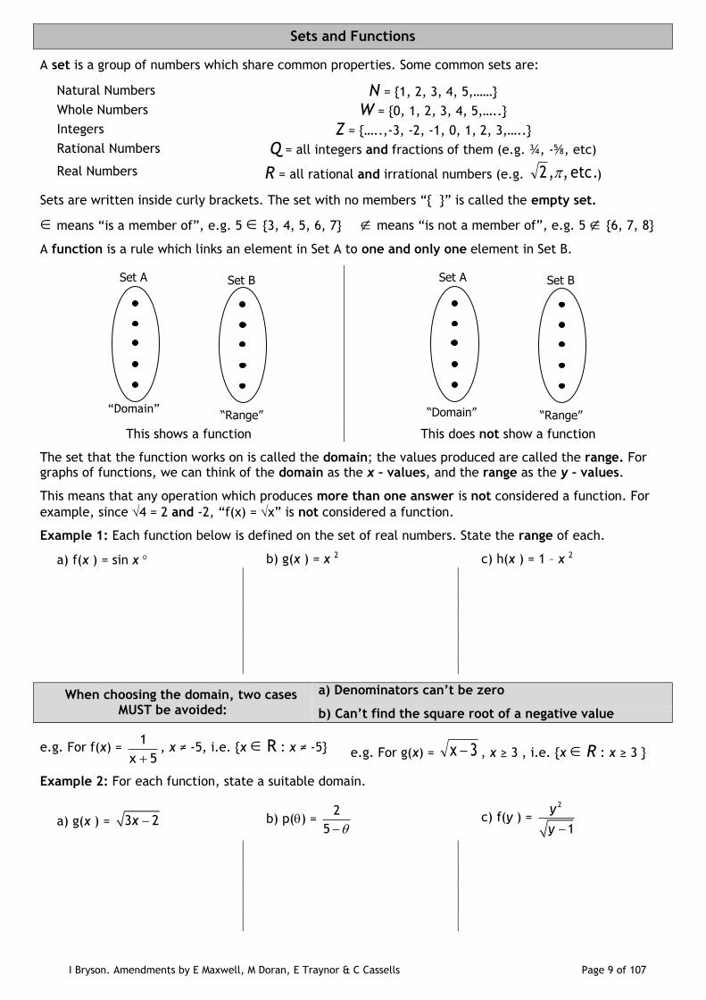
A function is a rule which links an element in Set A to one and only one element in Set B.
This shows a function This does not show a function
The set that the function works on is called the domain; the values produced are called the range. For graphs of functions, we can think of the domain as the x – values, and the range as the y – values.
This means that any operation which produces more than one answer is not considered a function. For
example, since 4 = 2 and -2, “f(x) = x” is not considered a function.
Example 1: Each function below is defined on the set of real numbers. State the range of each.
a) f(x ) = sin x b) g(x ) = x 2 c) h(x ) = 1 – x 2
When choosing the domain, two cases MUST be avoided:
a) Denominators can’t be zero
b) Can’t find the square root of a negative value
e.g. For f(x) = 5x
1
, x ≠ -5, i.e. {x R : x ≠ -5} e.g. For g(x) = 3x , x ≥ 3 , i.e. {x R : x ≥ 3 }
Example 2: For each function, state a suitable domain.
a) g(x ) = 3 2x b) p() = 2
5 c) f(y ) =
2
1
y
y
Set A Set B
“Domain” “Range”
Set A Set B
“Domain” “Range”
I Bryson. Amendments by E Maxwell, M Doran, E Traynor & C Cassells Page 10 of 107
Composite Functions
In the linear function y = 3x – 5, we get y by doing two acts: (i) multiply x by 3; (ii) then subtract 5. This is called a composite function, where we “do” a function to the range of another function.
e.g. If h(x) is the composite function obtained by performing f(x) on g(x), then we say
h(x) = f(g(x)) (“f of g of x”)
Example 3: f(x) = 5x + 1 and g(x) = 3x 2 + 2x .
a) Find f(g(-1)) b) Find f(g(x))
c) Find f(f(x)) d) Find g(f(x))
NOTE: Usually, f(g(x)) and g(f(x)) are NOT the same!
Example 4: f(x) = 2x + 1, g(x) = x2 + 6
a) Find formulae for: b) Solve the equation f(g(x)) = g(f(x))
(i) f(g(x))
(ii) g(f(x))
Example 5: f(x) = 1x
3
, x ≠ -1. Find an expression for f(f(x )), as a fraction in its simplest form.
I Bryson. Amendments by E Maxwell, M Doran, E Traynor & C Cassells Page 11 of 107
Past Paper Example: Functions f and g are defined on a set of real numbers by
2 3f x x 4g x x
a) Find expressions for:
(i) f(g(x)) (ii) g(f(x)) b) Show that f(g(x)) + g(f(x)) = 0 has no real roots
I Bryson. Amendments by E Maxwell, M Doran, E Traynor & C Cassells Page 12 of 107
Recurrence Relations
A recurrence relation is a rule which produces a sequence of numbers where each term is obtained from the previous one. Recurrence relations can be used to solve problems involving systems which grow or shrink by the same amount at regular intervals (e.g. the amount of money in a savings account which grows by 3.5% p/a, the volume of water left in a pool if 10% evaporates each day, etc).
Recurrence relations are generally written in one of two forms:
n 1 nU aU b
In both cases, a term is found by multiplying the previous term by a constant a, then adding (or subtracting) another constant b.
OR Un means the nth term in the sequence (i.e. U7 would be the 7th term, etc). U0 (“U zero”) is the starting point of the sequence, e.g. the amount of money put into an account before interest is added.
bUaU 1n-n
Example 1: A sequence is defined by the recurrence relation Un+1 = 3Un +2, U0 = 4.
Example 2: A sequence is defined by the recurrence relation Un = 4Un – 1 – 3, where U0 = a.
Find the value of U4. Find an expression for U2 in terms of a.
Finding a Formula
Recurrence relations can be used to describe situations seen in real life where a quantity changes by the same percentage at regular intervals. The first thing to do in most cases is find a formula to describe the situation.
Example: Jennifer puts £5000 into a high-interest savings account which pays 7.5% p/a. Find a recurrence relation for the amount of money in the savings account.
Solution: Starting amount = £5000 After 1 year: amount = starting amount + 7.5% (i.e. 107.5% of starting amount) = 1.075 x starting amount
Recurrence relation is: Un+1 = 1.075Un (U0 = 5000)
Example 3: Find a recurrence relation to describe:
a) The amount left to pay on a loan of £10000, with interest charged at 1.5% per month and fixed monthly payments of £250.
b) The amount of water in a swimming pool of volume 750,000 litres if 0.05% per day is lost to evaporation, but 350 litres extra is added daily.
Example 4: Bill puts lottery winnings of £120000 in a bank account which pays 5% interest p/a. After a year, he decides to spend £20000 per year from the money in the account.
a) Find a recurrence relation to describe the amount of money left each year.
I Bryson. Amendments by E Maxwell, M Doran, E Traynor & C Cassells Page 13 of 107
b) How much money will there be in the account after five years?
c) After how many years will Bill’s money run out?
Limits of Recurrence Relations
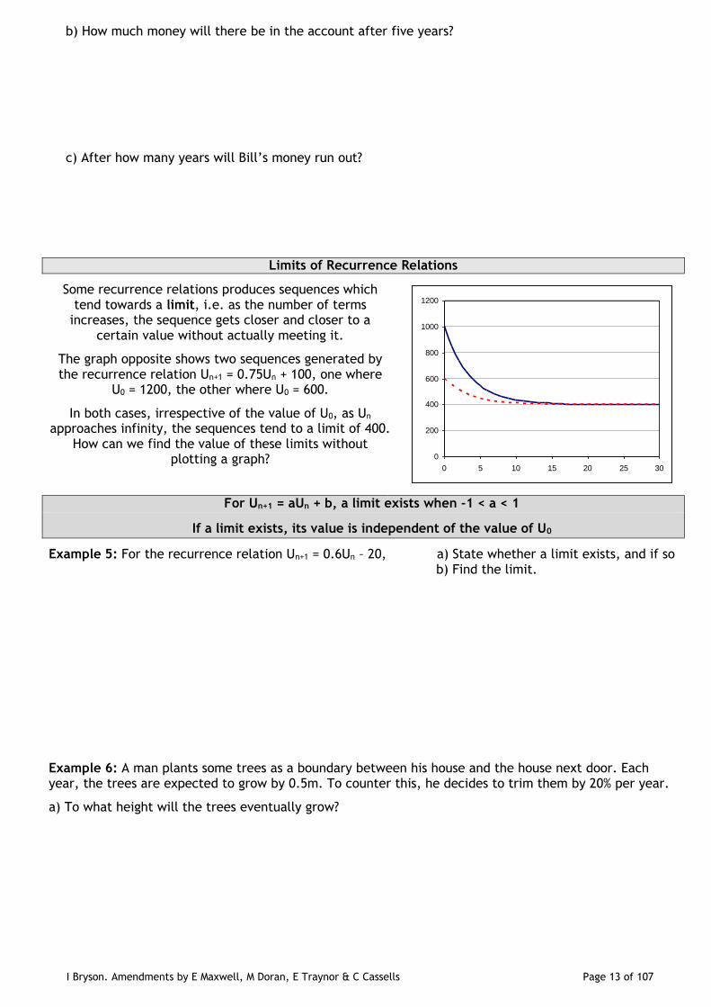
Some recurrence relations produces sequences which tend towards a limit, i.e. as the number of terms
increases, the sequence gets closer and closer to a certain value without actually meeting it.
The graph opposite shows two sequences generated by the recurrence relation Un+1 = 0.75Un + 100, one where
U0 = 1200, the other where U0 = 600.
In both cases, irrespective of the value of U0, as Un approaches infinity, the sequences tend to a limit of 400.
How can we find the value of these limits without plotting a graph?
For Un+1 = aUn + b, a limit exists when -1 < a < 1
If a limit exists, its value is independent of the value of U0
Example 5: For the recurrence relation Un+1 = 0.6Un – 20, a) State whether a limit exists, and if so b) Find the limit.
Example 6: A man plants some trees as a boundary between his house and the house next door. Each year, the trees are expected to grow by 0.5m. To counter this, he decides to trim them by 20% per year.
a) To what height will the trees eventually grow?
0
200
400
600
800
1000
1200
0 5 10 15 20 25 30
I Bryson. Amendments by E Maxwell, M Doran, E Traynor & C Cassells Page 14 of 107
b) His neighbour is unhappy that the trees are too tall, and insists they grow no taller than 2m high. What is the minimum percentage they must be trimmed each year to meet this condition?
Solving Recurrence Relations to Find a and b
If we have three consecutive terms in a sequence, we can find the values of a and b in the recurrence relation which generated the sequence using simultaneous equations.
Example 7: A sequence is generated by a recurrence relation of the form Un+1 = aUn + b. In this sequence, U1 = 28, U2 = 32 and U3 = 38. Find the values of a and b.
Past Paper Example: Marine biologists calculate that when the concentration of a particular chemical in a loch reaches 5 milligrams per litre (mg/L) the level of pollution endangers the lives of the fish.
A factory wishes to release waste containing this chemical into the loch, and supplies the Scottish Environmental Protection Agency with the following information:
1. The loch contains none of the chemical at present.
2. The company will discharge waste once per week which will result in an increase in concentration of 2.5 mg/L of the chemical in the loch.
3. The natural tidal action in the loch will remove 40% of the loch every week.
a) After how many weeks at this level of discharge will the lives of the fish become endangered?
b) The company offers to install a cleaning process which would result in an increase in concentration of only 1.75 mg/L of the chemical in the loch, and claim this will not endanger the lives of the fish in the long term.
Should permission be given to allow the company to discharge waste into the loch using this revised process? Justify your answer.
I Bryson. Amendments by E Maxwell, M Doran, E Traynor & C Cassells Page 15 of 107
Graphs of Functions
Sketching a Quadratic Graph (Revision)
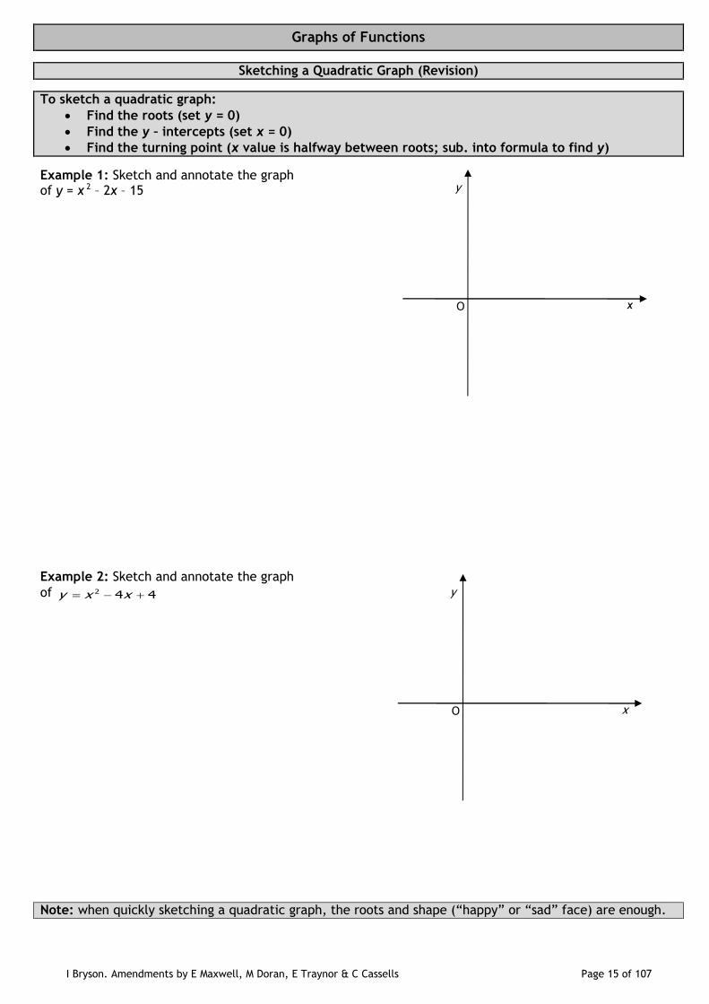
To sketch a quadratic graph:
Find the roots (set y = 0)
Find the y – intercepts (set x = 0)
Find the turning point (x value is halfway between roots; sub. into formula to find y)
Example 1: Sketch and annotate the graph of y = x 2 – 2x – 15
Example 2: Sketch and annotate the graph
of 2 4 4y x x
Note: when quickly sketching a quadratic graph, the roots and shape (“happy” or “sad” face) are enough.
y
x O
y
x O
I Bryson. Amendments by E Maxwell, M Doran, E Traynor & C Cassells Page 16 of 107
Graphs of Functions
Sketching Graphs (Revision)
In the exam, diagrams are provided whenever the question involves a graph. However, this is not the case when working from the textbook: it is therefore important that we are able to sketch basic graphs where
necessary, as often the question becomes simpler when you can see it.
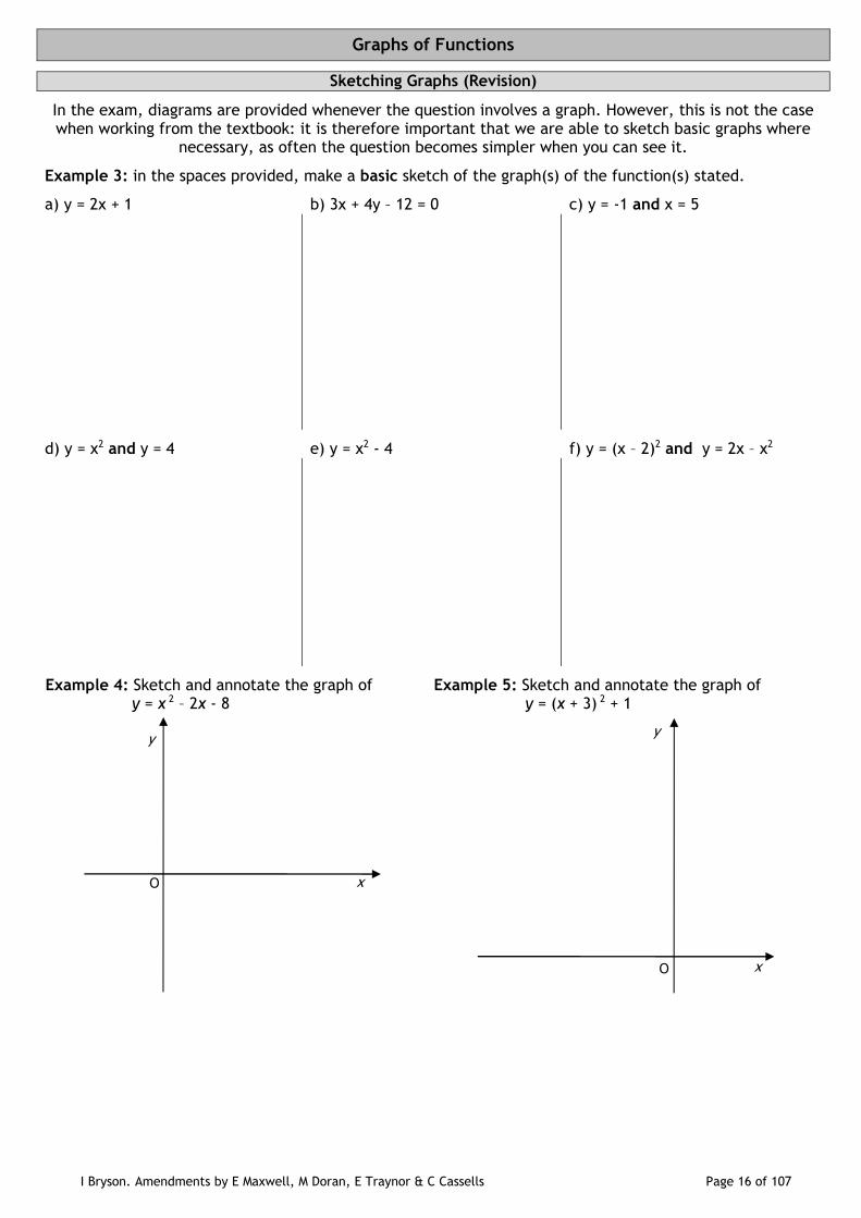
Example 3: in the spaces provided, make a basic sketch of the graph(s) of the function(s) stated.
a) y = 2x + 1 b) 3x + 4y – 12 = 0 c) y = -1 and x = 5
d) y = x2 and y = 4 e) y = x2 - 4 f) y = (x – 2)2 and y = 2x – x2
Example 4: Sketch and annotate the graph of y = x 2 – 2x - 8
Example 5: Sketch and annotate the graph of y = (x + 3) 2 + 1
y
x O
y
x O
I Bryson. Amendments by E Maxwell, M Doran, E Traynor & C Cassells Page 17 of 107
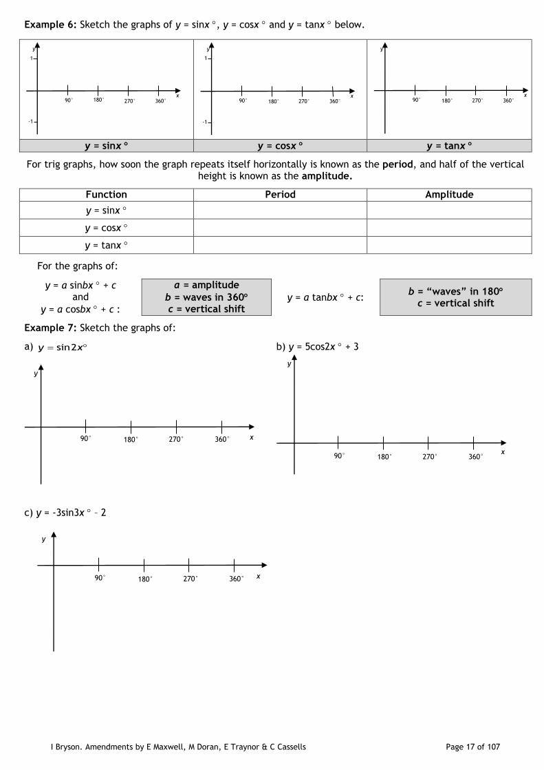
Example 6: Sketch the graphs of y = sinx , y = cosx and y = tanx below.
y = sinx y = cosx y = tanx
For trig graphs, how soon the graph repeats itself horizontally is known as the period, and half of the vertical height is known as the amplitude.
Function Period Amplitude
y = sinx
y = cosx
y = tanx
For the graphs of:
y = a sinbx + c and
y = a cosbx + c :
a = amplitude
b = waves in 360 c = vertical shift
y = a tanbx + c: b = “waves” in 180
c = vertical shift
Example 7: Sketch the graphs of:
a) sin2y x b) y = 5cos2x + 3
c) y = -3sin3x – 2
90° 180° 270° 360° x
y
1
-1
90° 180° 270° 360° x
y
1
-1
90° 180° 270° 360° x
y
90° 180° 270° 360°
y
x
y
90° 180° 270° 360°
90° 180° 270° 360°
y
x
x
I Bryson. Amendments by E Maxwell, M Doran, E Traynor & C Cassells Page 18 of 107
Compound Angles
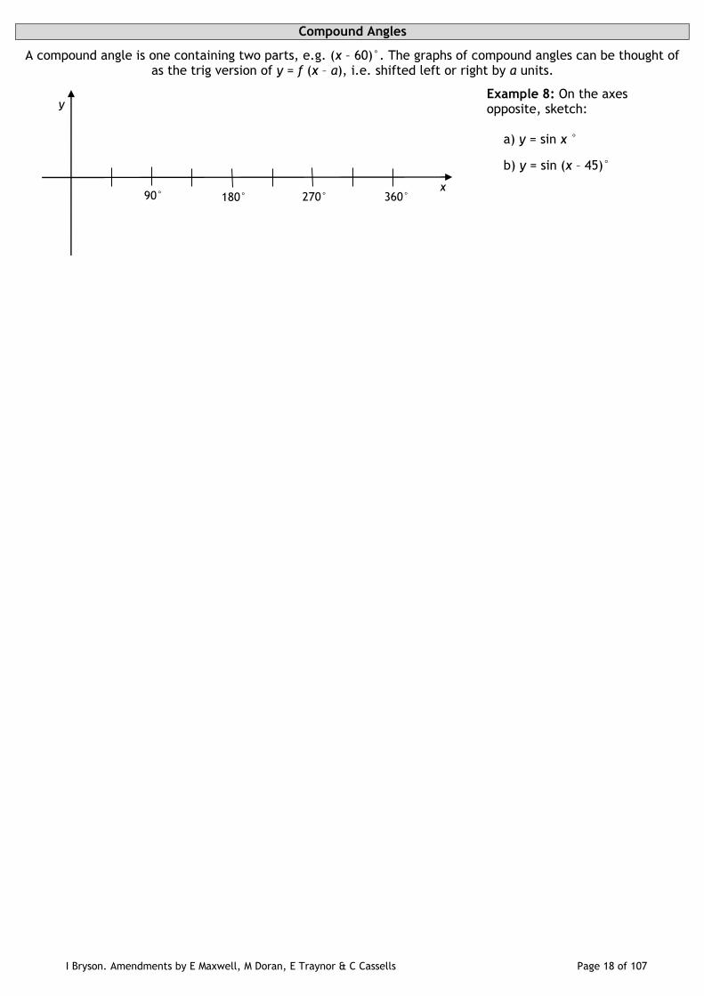
A compound angle is one containing two parts, e.g. (x – 60)°. The graphs of compound angles can be thought of as the trig version of y = f (x – a), i.e. shifted left or right by a units.
Example 8: On the axes opposite, sketch:
a) y = sin x °
b) y = sin (x – 45)°
90° 180° 270° 360° x
y
I Bryson. Amendments by E Maxwell, M Doran, E Traynor & C Cassells Page 19 of 107
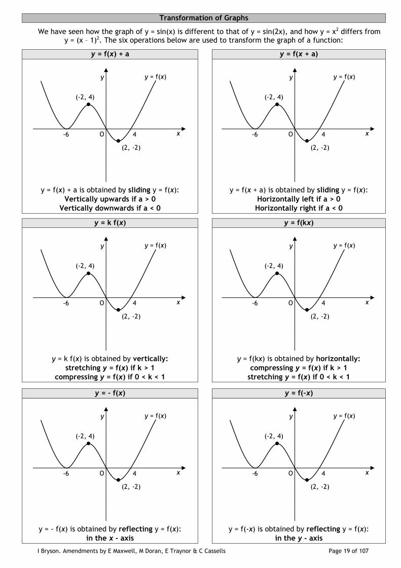
Transformation of Graphs
We have seen how the graph of y = sin(x) is different to that of y = sin(2x), and how y = x2 differs from y = (x – 1)2. The six operations below are used to transform the graph of a function:
y = f(x) + a y = f(x + a)
y = f(x) + a is obtained by sliding y = f(x): y = f(x + a) is obtained by sliding y = f(x):
Vertically upwards if a > 0 Horizontally left if a > 0
Vertically downwards if a < 0 Horizontally right if a < 0
y = k f(x) y = f(kx)
y = k f(x) is obtained by vertically: y = f(kx) is obtained by horizontally:
stretching y = f(x) if k > 1 compressing y = f(x) if k > 1
compressing y = f(x) if 0 < k < 1 stretching y = f(x) if 0 < k < 1
y = - f(x) y = f(-x)
y = - f(x) is obtained by reflecting y = f(x): y = f(-x) is obtained by reflecting y = f(x):
in the x - axis in the y - axis
x
y
O
(-2, 4)
y = f(x)
(2, -2)
4 -6 x
y
O
(-2, 4)
y = f(x)
(2, -2)
4 -6
x
y
O
(-2, 4)
y = f(x)
(2, -2)
4 -6 x
y
O
(-2, 4)
y = f(x)
(2, -2)
4 -6
x
y
O
(-2, 4)
y = f(x)
(2, -2)
4 -6 x
y
O
(-2, 4)
y = f(x)
(2, -2)
4 -6

I Bryson. Amendments by E Maxwell, M Doran, E Traynor & C Cassells Page 20 of 107
Multiple Transformations
Often, are asked to perform more than one transformation on a graph. Where appropriate, always leave sliding vertically to last.
Example 9: Part of the graph of y = f(x) is shown.
On separate diagrams, sketch:
a) y = f(-x) + 2
b) y = 2
1 f(x + 1)
Past Paper Example: The diagram shows a sketch of the function y = f(x ).
To the diagram, add the graphs of:
a) y = f(2x)
b) y = 1 – f(2x).
x
y
O
(-2, -4)
y = f(x)
(1, 1)
2 -3
x
y
O x
y
O
(-4, 8) (2, 8)
x
y
O

I Bryson. Amendments by E Maxwell, M Doran, E Traynor & C Cassells Page 21 of 107
Quadratic Functions
Finding the Equation of a Quadratic Function From Its Graph: y = k(x – a)(x – b)
If the graph of a quadratic function has roots at x = -1 and x = 5, a reasonable guess at its equation would be
y = x 2 – 4x – 5, i.e. from y = (x + 1)(x – 5).
However, as the diagram shows, there are many parabolas which pass through these points, all of which belong to the family of functions y = k (x + 1) (x – 5).
To find the equation of the original function, we need the roots and one other point on the curve (to allow us to
determine the value of k).
Example 1: State the equation of the graph below in the form y = ax 2 + bx + c .
Completing the Square (Revision)
The diagram shows the graphs of two quadratic functions.
If the graph of y = x 2 is shifted q units to the right, followed by r units up, then the graph of y = (x – q) 2 + r is
obtained.
As the turning point of y = x 2 is (0, 0), it follows that the new curve has a turning point at (q , r).
A quadratic equation written as y = p (x - q) 2 + r is said to be in the completed square form.
Example 2: (i) Write the following in the form y = (x + q) 2 + r and find the minimum value of y.
(ii) Hence state the minimum value of y and the corresponding value of x .
a) y = x 2 + 6x + 10 b) y = x 2 - 3x + 1
y
x
y
x 1 3
6
y
x
y = x 2
y = (x – q) 2 + r
(0, 0)
(q, r)
I Bryson. Amendments by E Maxwell, M Doran, E Traynor & C Cassells Page 22 of 107
Completing the Square when the x2 Coefficient ≠ 1
Example 3: Write y = 3x 2 + 12x + 5 in the form y = p(x + q) 2 + r.
Example 4: Write y = 5 + 12x – x 2 in the form y = p - (x + q) 2.
Example 5:
a) Write y = x 2 - 10x + 28 in the form y = (x + p) 2 + q.
b) Hence find the maximum value of 28 10x - x
182
Solving Quadratic Equations via Completing the Square
Quadratic equations which do not easily factorise can be solved in two ways: (i) completing the square, or (ii) using the quadratic formula. In fact, both methods are essentially the same, as the
quadratic formula is obtained by solving y = ax 2 + bx + c via completing the square.
Example 6: State the exact values of the roots of the equation 2x 2 - 4x + 1 = 0 by:
a) using the quadratic formula b) completing the square
I Bryson. Amendments by E Maxwell, M Doran, E Traynor & C Cassells Page 23 of 107
Solving Quadratic Inequations
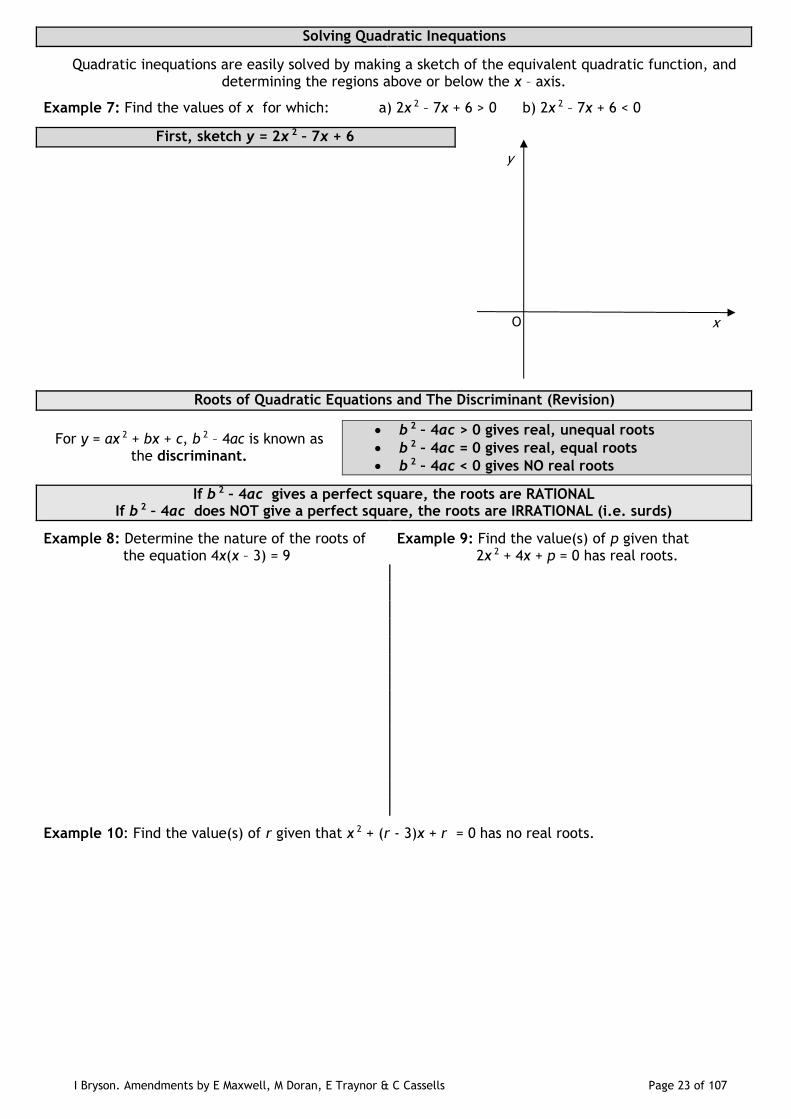
Quadratic inequations are easily solved by making a sketch of the equivalent quadratic function, and determining the regions above or below the x – axis.
Example 7: Find the values of x for which: a) 2x 2 – 7x + 6 > 0 b) 2x 2 – 7x + 6 < 0
First, sketch y = 2x 2 – 7x + 6
Roots of Quadratic Equations and The Discriminant (Revision)
For y = ax 2 + bx + c, b 2 – 4ac is known as the discriminant.
b 2 – 4ac > 0 gives real, unequal roots
b 2 – 4ac = 0 gives real, equal roots
b 2 – 4ac < 0 gives NO real roots
If b 2 – 4ac gives a perfect square, the roots are RATIONAL If b 2 – 4ac does NOT give a perfect square, the roots are IRRATIONAL (i.e. surds)
Example 8: Determine the nature of the roots of the equation 4x(x – 3) = 9
Example 9: Find the value(s) of p given that 2x 2 + 4x + p = 0 has real roots.
Example 10: Find the value(s) of r given that x 2 + (r - 3)x + r = 0 has no real roots.
y
x O
I Bryson. Amendments by E Maxwell, M Doran, E Traynor & C Cassells Page 24 of 107
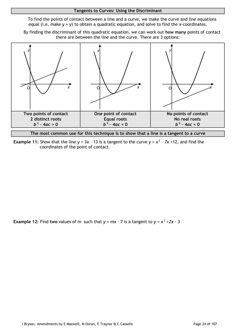
Tangents to Curves: Using the Discriminant
To find the points of contact between a line and a curve, we make the curve and line equations equal (i.e. make y = y) to obtain a quadratic equation, and solve to find the x-coordinates.
By finding the discriminant of this quadratic equation, we can work out how many points of contact there are between the line and the curve. There are 3 options:
Two points of contact One point of contact No points of contact
2 distinct roots Equal roots No real roots
b 2 – 4ac > 0 b 2 – 4ac = 0 b 2 – 4ac < 0
The most common use for this technique is to show that a line is a tangent to a curve
Example 11: Show that the line y = 3x – 13 is a tangent to the curve y = x 2 – 7x +12, and find the coordinates of the point of contact.
Example 12: Find two values of m such that y = mx - 7 is a tangent to y = x 2 +2x – 3
y
x O
y
x O
y
x O
I Bryson. Amendments by E Maxwell, M Doran, E Traynor & C Cassells Page 25 of 107
Past Paper Example 1: Express 2x2 + 12x + 1 in the form a(x + b)2 + c.
Past Paper Example 2: Given that 2x2 + px + p + 6 = 0 has no real roots, find the range of values for p.
Past Paper Example 3: Show that the roots of (k – 2)x 2 – 3kx + 2k = -2x are always real.

I Bryson. Amendments by E Maxwell, M Doran, E Traynor & C Cassells Page 26 of 107
The Circle
If we draw, suitable to relative axes, a circle, radius r, centred on the origin, then the distance from
the centre of any point P (x, y) could be determined to be 22 yxd .
As the shape is a circle, then this distance is equal to the radius. It therefore follows that:
Since 22 yxr , then 222 yxr
Therefore,
The equation x 2 + y 2 = r 2 describes a circle with centre (0, 0) and radius r
Example 1: Write down the centre and radius of each circle.
a) x 2 + y 2 = 64 b) x 2 + y 2 = 361 c) x 2 + y 2 = 25
3
Example 2: State where the points (-2, 7), (6, -8) and (5, 9) lie in relation to the circle x 2 + y 2 = 100.
Circles with Centres Not at the Origin
The radius in the above circle is the distance between (x , y ) and
the origin, i.e. 22 0)-(y0)-(xr . If we move the centre to the
point (a , b), then 22 b)-(ya)-(xr .
Squaring both sides, we can now also say that:
The equation (x – a) 2 + (y – b) 2 = r 2 describes a circle with centre (a, b) and radius r
Example 3: Write down the centre and radius of each circle.
a) (x – 1) 2 + (y + 3) 2 = 4 b) (x + 9) 2 + (y - 2) 2 = 20 c) (x – 5) 2 + y 2 = 400
P (x, y)
x
y
O
r
P (x, y)
x
y
O
r
C (a, b)

I Bryson. Amendments by E Maxwell, M Doran, E Traynor & C Cassells Page 27 of 107
Example 4: A is the point (4, 9) and B is the point (-2, 1). Find the equation of the circle for which AB is the diameter.
Example 5: Points P, Q and R have coordinates (-10, 2), (5, 7) and (6, 4) respectively.
a) Show that triangle PQR is right angled at Q. b) Hence find the equation of the circle passing through points P, Q and R.
The General Equation of a Circle
For the circle described in Example 3a, we could expand the brackets and simplify to obtain the equation x 2 + y 2 – 2x + 6y + 6 = 0, which would also describe a circle with centre (1, -3) and radius 2.
For x 2 + y 2 + 2gx + 2fy + c = 0, Therefore, the circle described by
(x 2 + 2gx) + (y 2 + 2fy) = - c x 2 + y 2 + 2gx + 2fy + c = 0
(x 2 + 2gx + g 2) + (y 2 + 2fy + f 2) = g 2 + f 2 - c has centre (-g, -f ) and r = cfg 22
(x + g)2 + (y + f )2 = (g 2 + f 2 – c)
Example 6: Find the centre and radius of the circle with equation x 2 + y 2 – 4x + 8y – 5 = 0
Example 7: State why the equation x 2 + y 2 – 4x – 4y + 15 = 0 does not represent a circle.
Example 8: State the range of values of c such that the equation x 2 + y 2 – 4x + 6y + c = 0 describes a circle.
Example 9: Find the equation of the circle concentric with x 2 + y 2 + 6x – 2y - 54 = 0 but with radius half its size.
I Bryson. Amendments by E Maxwell, M Doran, E Traynor & C Cassells Page 28 of 107
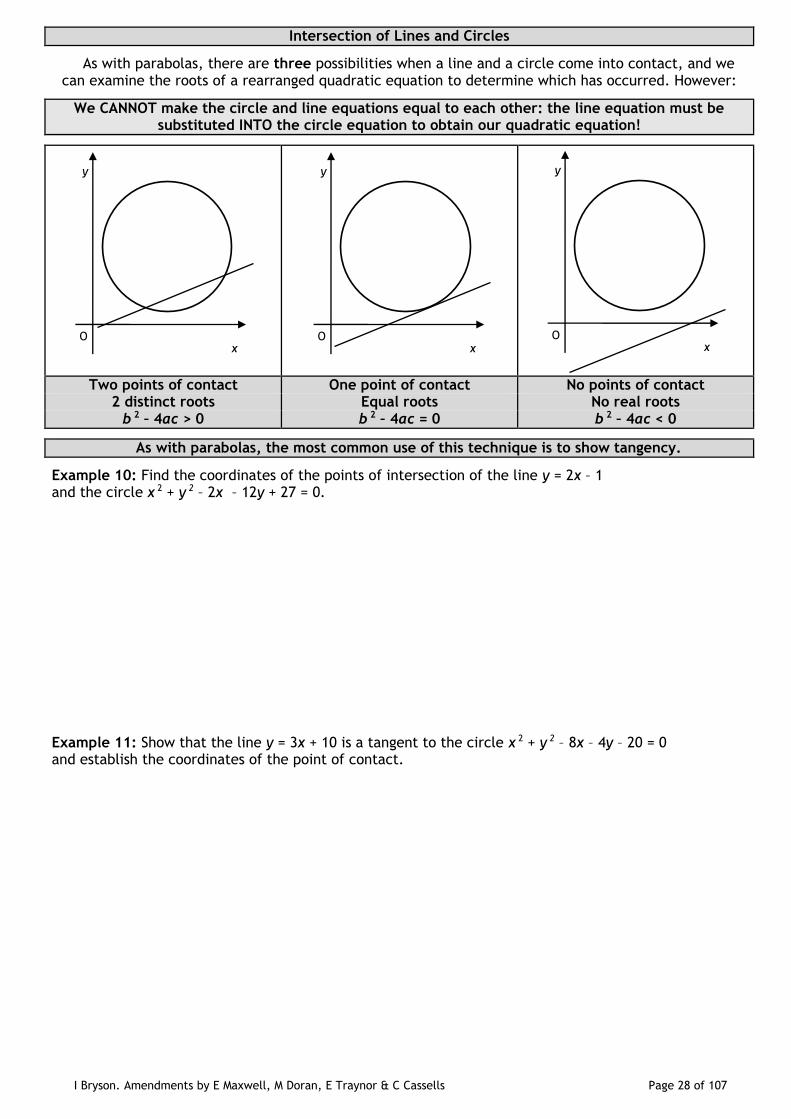
Intersection of Lines and Circles
As with parabolas, there are three possibilities when a line and a circle come into contact, and we can examine the roots of a rearranged quadratic equation to determine which has occurred. However:
We CANNOT make the circle and line equations equal to each other: the line equation must be substituted INTO the circle equation to obtain our quadratic equation!
Two points of contact One point of contact No points of contact
2 distinct roots Equal roots No real roots b 2 – 4ac > 0 b 2 – 4ac = 0 b 2 – 4ac < 0
As with parabolas, the most common use of this technique is to show tangency.
Example 10: Find the coordinates of the points of intersection of the line y = 2x – 1 and the circle x 2 + y 2 – 2x – 12y + 27 = 0.
Example 11: Show that the line y = 3x + 10 is a tangent to the circle x 2 + y 2 – 8x – 4y – 20 = 0 and establish the coordinates of the point of contact.
y
x O
y
x O
y
x O
I Bryson. Amendments by E Maxwell, M Doran, E Traynor & C Cassells Page 29 of 107
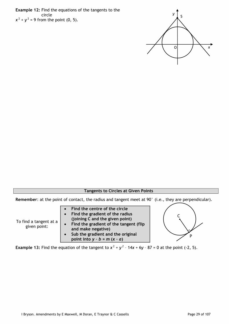
Example 12: Find the equations of the tangents to the circle
x 2 + y 2 = 9 from the point (0, 5).
Tangents to Circles at Given Points
Remember: at the point of contact, the radius and tangent meet at 90° (i.e., they are perpendicular).
To find a tangent at a given point:
Find the centre of the circle
Find the gradient of the radius (joining C and the given point)
Find the gradient of the tangent (flip and make negative)
Sub the gradient and the original point into y – b = m (x – a)
Example 13: Find the equation of the tangent to x 2 + y 2 – 14x + 6y – 87 = 0 at the point (-2, 5).
x
y
O
5
C
P
I Bryson. Amendments by E Maxwell, M Doran, E Traynor & C Cassells Page 30 of 107
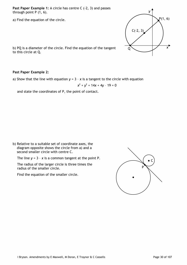
Past Paper Example 1: A circle has centre C (-2, 3) and passes through point P (1, 6).
a) Find the equation of the circle.
b) PQ is a diameter of the circle. Find the equation of the tangent to this circle at Q.
Past Paper Example 2:
a) Show that the line with equation y = 3 – x is a tangent to the circle with equation
x2 + y2 + 14x + 4y – 19 = 0
and state the coordinates of P, the point of contact.
b) Relative to a suitable set of coordinate axes, the diagram opposite shows the circle from a) and a second smaller circle with centre C.
The line y = 3 – x is a common tangent at the point P.
The radius of the larger circle is three times the radius of the smaller circle.
Find the equation of the smaller circle.
P(1, 6)
C(-2, 3)
x
y
Q
●
● C
P
●
I Bryson. Amendments by E Maxwell, M Doran, E Traynor & C Cassells Page 31 of 107
Past Paper Example 3: Given that the equation
x2 + y2 – 2px – 4py + 3p + 2 = 0
represents a circle, determine the range of values of p.
Past Paper Example 4: Circle P has equation2 2 8 10 9 0x y x y . Circle Q has centre (-2, -1) and
radius 2 2 .
a) i) Show that the radius of circle P is 4 2 . ii) Hence show that circles P and Q touch. b) Find the equation of the tangent to circle Q at the point (-4, 1)

I Bryson. Amendments by E Maxwell, M Doran, E Traynor & C Cassells Page 32 of 107
Calculus 1: Differentiation
In the chapter on straight lines, we saw that the gradient of a line is a measure of how quickly
it increases (or decreases) at a constant rate.
This is easy to see for linear functions, but what about quadratic, cubic and higher functions? As these functions produce curved graphs, they do
not increase or decrease at a constant rate.
For a function f(x), the rate of change at any point on the function can be found by measuring
the gradient of a tangent to the curve at that point.
The rate of change at any point of a function is called the derived function or the derivative.
Finding the rate of change of a function at a given point is part of a branch of maths known as calculus.
For function f(x) or the graph y = f(x), the derivative is written as:
f'(x) (“f dash x”)
OR
dx
dy (“dy by dx”)
Derivative = Rate of Change of the Function = Gradient of the Tangent to the Curve
The Derivative of f(x) = ax n
Example 1: Find the derivative of f(x) = x 2 To find the derivative of a function:
1. Make sure it’s written in the form y = ax n 2. Multiply by the power 3. Decrease the power by one
Example 2: f(x) = 2x 3. Find f’(x ). This means:
At x = 1, the gradient of the tangent to 2x 3 =
At x = -2, the gradient of the tangent to 2x 3 =
If f(x) = ax n, then f’(x) = nax n-1 The DE rivative DE creases the power!
To find the derivative of f(x):
f(x) MUST be written in the form f(x) = ax n
Rewrite to eliminate fractions by using negative indices
Rewrite to eliminate roots by using fractional indices
Revision from National 5
Example 3: Write with negative indices: Example 4: Write in index form:
a) 2x
2 b)
54x
1 c)
5x
3 a) x b) 3 2x
c) 7x3
2
x
y
O
I Bryson. Amendments by E Maxwell, M Doran, E Traynor & C Cassells Page 33 of 107
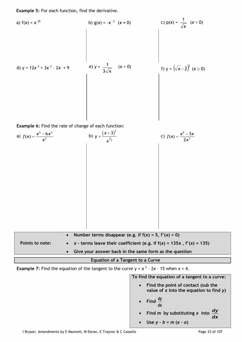
Example 5: For each function, find the derivative.
a) f(x) = x 35 b) g(x) = -x -3 (x ≠ 0) c) p(x) = 1
x (x > 0)
d) y = 12x 5 + 3x 2 – 2x + 9 e) y = x3
1 (x > 0) f) y = 22x (x 0)
Example 6: Find the rate of change of each function:
a) 5 3
2
6( )
x xf x
x
b)
2
23
3xy
x
c)
5
3
3( )
2
x xf x
x
Points to note:
Number terms disappear (e.g. if f(x) = 5, f’(x) = 0)
x – terms leave their coefficient (e.g. if f(x) = 135x , f’(x) = 135)
Give your answer back in the same form as the question
Equation of a Tangent to a Curve
Example 7: Find the equation of the tangent to the curve y = x 2 – 2x – 15 when x = 4.
To find the equation of a tangent to a curve:
Find the point of contact (sub the value of x into the equation to find y)
Find dx
dy
Find m by substituting x into dx
dy
Use y – b = m (x – a)

I Bryson. Amendments by E Maxwell, M Doran, E Traynor & C Cassells Page 34 of 107
Example 8:
a) Find the gradient of the tangent to the curve
y = x 3 – 2x 2 at the point where x = 3
7.
b) Find the other point on the curve where the tangent has the same gradient.
Example 9: Find the point of contact of the tangent to the curve with equation 2 7 3y x x when the
gradient of the tangent is 9.
Stationary Points and their Nature
Any point on a curve where the tangent is horizontal (i.e. the gradient or dx
dy= 0) is commonly known as
a stationary point. There are four types of stationary point:
Minimum
Turning Point Maximum
Turning Point Rising
Point of Inflection Falling
Point of Inflection
To locate the position of stationary points, we find the derivative, make it equal zero, and solve for x. To determine their type (or nature), we must use a nature table.
O
f(x)
x O
f(x)
x O
f(x)
x O
f(x)

I Bryson. Amendments by E Maxwell, M Doran, E Traynor & C Cassells Page 35 of 107
Example 10: Find the stationary points of the curve y = 2x 3 – 12x 2 + 18x and determine their nature.

I Bryson. Amendments by E Maxwell, M Doran, E Traynor & C Cassells Page 36 of 107
Increasing & Decreasing Functions
For any curve,
if dx
dy> 0, then y is increasing
if dx
dy< 0, then y is decreasing
if dx
dy= 0, then y is stationary
If a function is always increasing (or decreasing), it is said to be strictly increasing (or decreasing).
Example 11: State whether the function f(x) = x 3 – x 2 – 5x + 2 is increasing, decreasing or stationary when:
Example 12: Show algebraically that the function f(x) = x 3 – 6x 2 + 12x – 5 is never decreasing.
a) x = 0
b) x = 1
c) x = 2
Example 13: Find the intervals in which the function f(x) = 2x 3 – 6x 2 + 5 is increasing and decreasing.
x
y
O
I Bryson. Amendments by E Maxwell, M Doran, E Traynor & C Cassells Page 37 of 107
Curve Sketching
To accurately sketch and annotate the curve obtained from a function, we must consider:
1. x – and y – intercepts 2. Stationary points and their nature
Example 14: Sketch and annotate fully y = x 3(4 – x)
I Bryson. Amendments by E Maxwell, M Doran, E Traynor & C Cassells Page 38 of 107
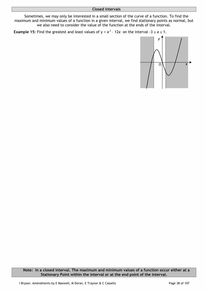
Closed Intervals
Sometimes, we may only be interested in a small section of the curve of a function. To find the maximum and minimum values of a function in a given interval, we find stationary points as normal, but
we also need to consider the value of the function at the ends of the interval.
Example 15: Find the greatest and least values of y = x 3 – 12x on the interval -3 ≤ x ≤ 1.
Note: In a closed interval. The maximum and minimum values of a function occur either at a Stationary Point within the interval or at the end point of the interval.
x
y
O

I Bryson. Amendments by E Maxwell, M Doran, E Traynor & C Cassells Page 39 of 107
Differentiation in Context: Optimisation
Differentiation can be used to find the maximum or minimum values of things which happen in real life. Finding the maximum or minimum value of a system is called optimisation.
Example 16: A carton is in the shape of a cuboid with a rectangular base and a volume of 3888cm3.
The surface area of the carton can be represented by the formula A(x) = 4x2 + x
5832.
Find the value of x such that the surface area is a minimum. In exams, optimisation questions almost always consist of two parts: part one asks you to show that a
situation can be described using an algebraic formula or equation, whilst part two asks you to use the given formula to find a maximum or minimum value by differentiation.
Leave part 1 of an optimisation question until the end of the exam (if you have time), as they are almost always (i) more difficult than finding the stationary point and (ii) worth fewer marks.
Remember that part 2 is just a well-disguised “find the minimum/maximum turning point of this function” question!
Example 17: A square piece of card of side 30cm has a square of side x cm cut from each corner. An open box is formed by turning up the sides.
a) Show that the volume, V , of the box may be expressed as 2 3900 120 4x x x
I Bryson. Amendments by E Maxwell, M Doran, E Traynor & C Cassells Page 40 of 107
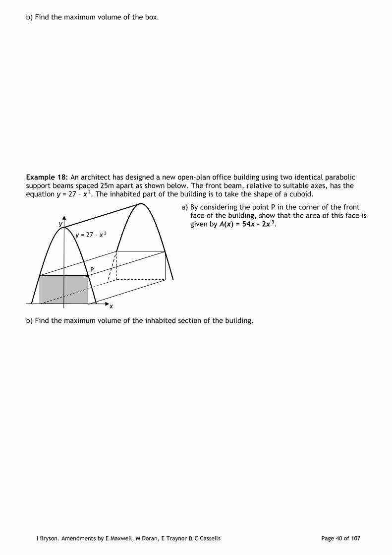
b) Find the maximum volume of the box.
Example 18: An architect has designed a new open-plan office building using two identical parabolic support beams spaced 25m apart as shown below. The front beam, relative to suitable axes, has the equation y = 27 – x 2. The inhabited part of the building is to take the shape of a cuboid.
a) By considering the point P in the corner of the front face of the building, show that the area of this face is given by A(x) = 54x – 2x 3.
b) Find the maximum volume of the inhabited section of the building.
P
y = 27 – x 2
x
y

I Bryson. Amendments by E Maxwell, M Doran, E Traynor & C Cassells Page 41 of 107
Graph of the Derived Function
From the graph of y = f(x), we can obtain the graph of y = f’(x) by considering its stationary points. On the graph of y = f’(x), the y-coordinate comes from the derivative of y = f(x).
1. Draw a set of axes directly under a copy of y = f(x).
2. Locate the stationary points.
3. At SP’s, f’(x) = 0, so the y coordinate of f’(x) = 0 on the new graph.
4. Where f(x) is increasing, f’(x) is above the x – axis.
5. Where f(x) is decreasing, f’(x) is below the x – axis.
6. Draw a smooth curve which fits this information.
Example 19: For the graphs below. Sketch the corresponding derived graphs of y = f’(x)
x
y
O
x O
y
y = f(x)
y
x
y
x
y = f(x)
a)
I Bryson. Amendments by E Maxwell, M Doran, E Traynor & C Cassells Page 42 of 107
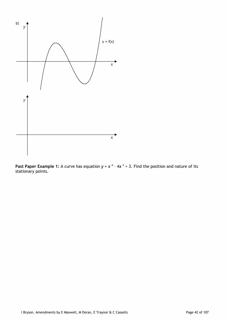
Past Paper Example 1: A curve has equation y = x 4 – 4x 3 + 3. Find the position and nature of its stationary points.
y
x
y
x
y = f(x)
b)
I Bryson. Amendments by E Maxwell, M Doran, E Traynor & C Cassells Page 43 of 107
Past Paper Example 2: Find the equation of the two tangents to the curve y = 2x 3 – 3x 2 – 12x + 20 which are parallel to the line 48x – 2y = 5.
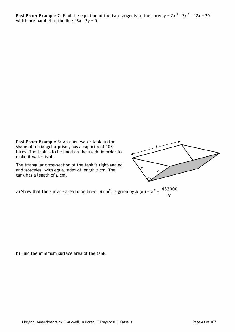
Past Paper Example 3: An open water tank, in the shape of a triangular prism, has a capacity of 108 litres. The tank is to be lined on the inside in order to make it watertight.
The triangular cross-section of the tank is right-angled and isosceles, with equal sides of length x cm. The tank has a length of L cm.
a) Show that the surface area to be lined, A cm2, is given by A (x ) = x 2 + x
432000
b) Find the minimum surface area of the tank.
x x
L

I Bryson. Amendments by E Maxwell, M Doran, E Traynor & C Cassells Page 44 of 107
Past Paper Example 4: A function is defined on the domain 0 x 3 by f(x) = x3 – 2x2 – 4x + 6.
Determine the maximum and minimum values of f.

I Bryson. Amendments by E Maxwell, M Doran, E Traynor & C Cassells Page 45 of 107
Calculus 2: Integration
The reverse process to differentiation is known as integration.
Differentiation
f(x) f’(x)
Integration
As it is the opposite of finding the derivative, the function obtained by integration is sometimes
called the anti-derivative, but is more commonly known as the integral, and is given the sign .
If f(x) = x n, then dxx n is “the integral of x n with respect to x ”
Indefinite Integrals and the Constant of Integration
Consider the three functions a(x) = 3x 2 + 2x + 5, b(x) = 3x 2 + 2x – 8 and c(x) = 3x 2 + 2x - 4
13.
In each case, the derivative of the function is the same, i.e. 6x + 2. This means that 2)dx(6x has
more than one answer. Because there is more than one answer, we say that this is an indefinite
integral, and we must include in the answer a constant value C, to represent the 5, -8, 4
13 etc which
we would need to distinguish a(x) from b(x) from c (x ) etc.
To find the integral of a function, we do the opposite of what we would do to find the derivative:
In general: 1)(nC1n
axdxax
1nn
IN tegration IN creases the power! 1. Write as ax n
2. Increase the power by 1 3. Divide by the new power
Example 1: Find (remember “+C”):
a) dx2x b) dt4t2 c) 4)dx(3x 5
f(x) f’(x) Multiply by
the old
power
Decrease the
power by 1
f(x) f’(x)
I Bryson. Amendments by E Maxwell, M Doran, E Traynor & C Cassells Page 46 of 107
d) dgg
34
(g ≠ 0) e) dpp6 5 3 f)
dyy
34y
32
(y ≠ 0)
The Definite Integral
A definite integral of a function is the difference between the integrals of f(x ) at two values of x . Suppose we integrate f(x ) and get F(x ). Then the integral of f(x ) when x = a would be F(a), and the
integral when x = b would be F(b).
The definite integral of f(x ), with respect to x , between a and b, is written as:
F(a)F(b)f(x)dxb
a
(where b > a)
For example, the integral of f(x ) = 2x 2 – 4 between the values x = -3 and x = 5 is written as
dx)4(2x5
3
2
and reads “the integral from -3 to 5 of 2x 2 – 4 with respect to x ”.
Note: definite integrals do NOT include the constant of integration!
)F(aF(b)C][F(a)C][F(b)f(x)b
a
Example 2: Evaluate 3
1dx1)(2x
To find a definite integral:
prepare the function for integration
integrate as normal, but write inside square brackets with the limits to the right
sub each limit into the integral, and subtract the integral with the lower limit from the one with the higher limit
Example 3: Evaluate dp1p1p2
0 Example 4: Evaluate
32 dx2x)-(x
1
I Bryson. Amendments by E Maxwell, M Doran, E Traynor & C Cassells Page 47 of 107
Example 5: Find the value of g such that g
2dx5)(6x = 6.
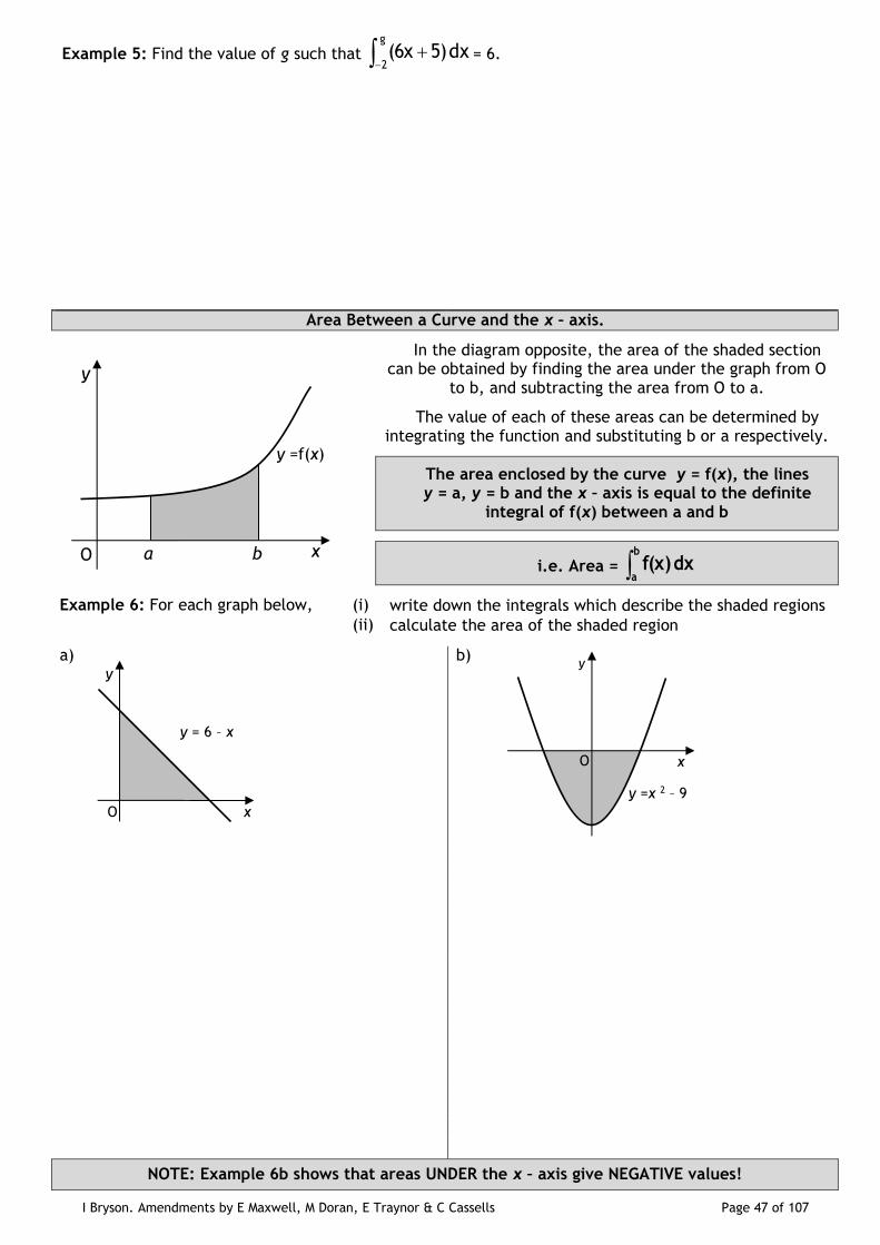
Area Between a Curve and the x – axis.
In the diagram opposite, the area of the shaded section can be obtained by finding the area under the graph from O
to b, and subtracting the area from O to a.
The value of each of these areas can be determined by integrating the function and substituting b or a respectively.
The area enclosed by the curve y = f(x), the lines y = a, y = b and the x – axis is equal to the definite
integral of f(x) between a and b
i.e. Area = b
adxf(x)
Example 6: For each graph below, (i) write down the integrals which describe the shaded regions
(ii) calculate the area of the shaded region
a)
b)
NOTE: Example 6b shows that areas UNDER the x – axis give NEGATIVE values!
x
y
O
y =f(x)
a b
x
y = 6 – x
y
O
x
y
y =x 2 – 9
O
I Bryson. Amendments by E Maxwell, M Doran, E Traynor & C Cassells Page 48 of 107
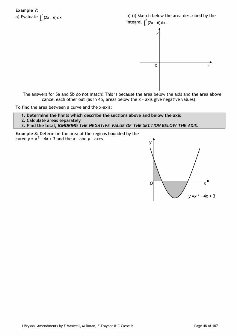
Example 7:
a) Evaluate dx)6(2x7
1 b) (i) Sketch below the area described by the
integral dx)6(2x7
1 .
The answers for 5a and 5b do not match! This is because the area below the axis and the area above cancel each other out (as in 4b, areas below the x – axis give negative values).
To find the area between a curve and the x-axis:
1. Determine the limits which describe the sections above and below the axis 2. Calculate areas separately 3. Find the total, IGNORING THE NEGATIVE VALUE OF THE SECTION BELOW THE AXIS.
Example 8: Determine the area of the regions bounded by the curve y = x 2 – 4x + 3 and the x – and y – axes.
y
x O
x
y
y =x 2 – 4x + 3
O
I Bryson. Amendments by E Maxwell, M Doran, E Traynor & C Cassells Page 49 of 107
Area Between Two Curves
Consider the area bounded by the curves y = (x – 2)2 and y = x .
Area = 3
1dxx -
3
1
2 dx2)(x
The diagrams above show that the area between the curves is equal to the area between the top function (x ) and the x – axis MINUS the area between the bottom curve ((x – 2) 2) and the x – axis.
The area between the curves y = f(x ) and y = g(x ) (which meet at the points where x = a and x = b ) is given by:
b
ag(x))dx(f(x)A
where: f(x) is the TOP function and g(x) is the
BOTTOM
b > a
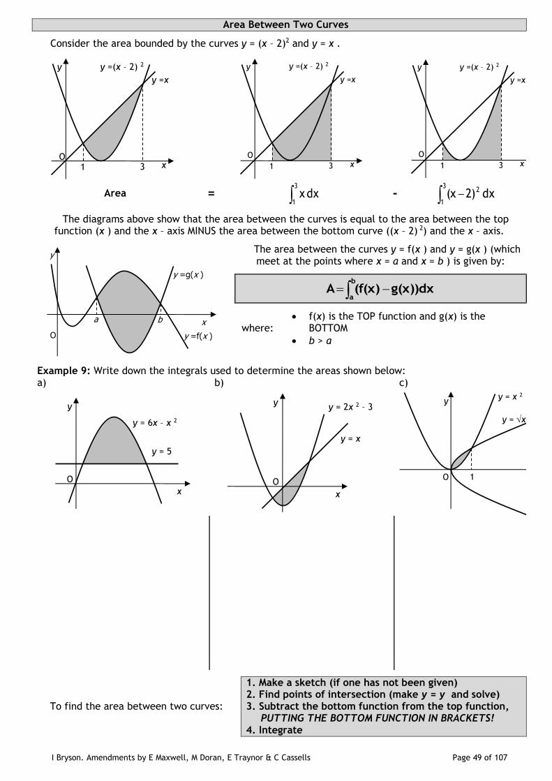
Example 9: Write down the integrals used to determine the areas shown below: a) b) c)
To find the area between two curves:
1. Make a sketch (if one has not been given) 2. Find points of intersection (make y = y and solve) 3. Subtract the bottom function from the top function, PUTTING THE BOTTOM FUNCTION IN BRACKETS! 4. Integrate
x
y y =(x – 2) 2
O
y =x
1 3 x
y y =(x – 2) 2
O
y =x
1 3 x
y y =(x – 2) 2
O
y =x
1 3
x
y
y =g(x )
O y =f(x )
a b
y = 6x – x 2
y
x
O
y = 5
y = 2x 2 – 3 y
x
O
y = x
y = x 2 y
x O 1
y = x
I Bryson. Amendments by E Maxwell, M Doran, E Traynor & C Cassells Page 50 of 107
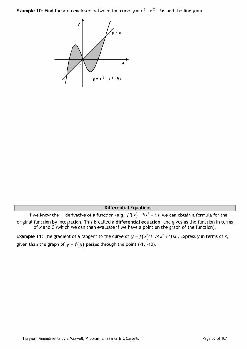
Example 10: Find the area enclosed between the curve y = x 3 – x 2 – 5x and the line y = x
Differential Equations
If we know the derivative of a function (e.g. 2' 6 3f x x ), we can obtain a formula for the
original function by integration. This is called a differential equation, and gives us the function in terms of x and C (which we can then evaluate if we have a point on the graph of the function).
Example 11: The gradient of a tangent to the curve of y f x is 224 10x x , Express y in terms of x,
given than the graph of y f x passes through the point (-1, -10).
y = x
y
x O
y = x 3 – x 2 – 5x
I Bryson. Amendments by E Maxwell, M Doran, E Traynor & C Cassells Page 51 of 107
Past Paper Example 1: Evaluate 9
1dx
x
1x
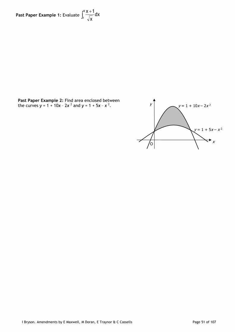
Past Paper Example 2: Find area enclosed between the curves y = 1 + 10x – 2x 2 and y = 1 + 5x – x 2.
y
x O
y = 1 + 10x – 2x 2
y = 1 + 5x – x 2
I Bryson. Amendments by E Maxwell, M Doran, E Traynor & C Cassells Page 52 of 107
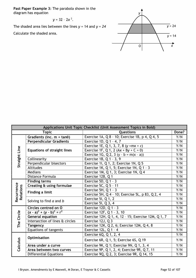
Past Paper Example 3: The parabola shown in the diagram has equation
y = 32 – 2x 2.
The shaded area lies between the lines y = 14 and y = 24
Calculate the shaded area.
Applications Unit Topic Checklist (Unit Assessment Topics in Bold)
Topic Questions Done?
Str
aig
ht
Lin
e
Gradients (inc. m = tan) Exercise 1A, Q 8 – 10; Exercise 1B, p 4, Q 4, 5 Y/N
Perpendicular Gradients Exercise 1D, Q 1 – 4, 7 Y/N
Equations of straight lines
Exercise 1E, Q 1, 3, 7, 8 (y =mx + c) Y/N
Exercise 1F, Q 1, 2 (Ax + By + C = 0) Y/N
Exercise 1G, Q 2, 3 (y – b = m(x – a)) Y/N
Collinearity Exercise 1B, Q 1 – 3, 9 Y/N
Perpendicular bisectors Exercise 1I, Q 1, 2; Exercise 1N, Q 5 Y/N
Altitudes Exercise 1K, Q 1, 5; Exercise 1N, Q 1 – 3 Y/N
Medians Exercise 1M, Q 1, 3; Exercise 1N, Q 4 Y/N
Distance Formula Exercise 12B, Q 1 Y/N
Recurr
ence
Rela
tions
Finding terms Exercise 5D, Q 1 – 3 Y/N
Creating & using formulae Exercise 5C, Q 5 – 11 Y/N
Finding a limit Exercise 5H, Q 1 – 3 Y/N
Exercise 5H, Q 4 – 10; Exercise 5L, p 83, Q 2, 4 Y/N
Solving to find a and b Exercise 5I, Q 1, 2 Y/N
Exercise 5I, Q 3, 4 Y/N
The C
ircle
Circles centred on O Exercise 12D, Q 1 – 3 Y/N
(x – a)2 + (y – b)2 = r2 Exercise 12F, Q 1 – 3, 10 Y/N
General equation Exercise 12H, Q 1, 4, 12 – 15; Exercise 12M, Q 1, 7 Y/N
Intersection of lines & circles Exercise 12J, Q 3 Y/N
Tangency Exercise 12K, Q 2, 6; Exercise 12M, Q 4, 8 Y/N
Equations of tangents Exercise 12L, Q 1 – 4 Y/N
Calc
ulu
s Optimisation Exercise 6Q, Q 1, 2, 4 Y/N
Exercise 6R, Q 1, 5; Exercise 6S, Q 19 Y/N
Area under a curve Exercise 9K, Q 1; Exercise 9N, Q 1, 3, 4 Y/N
Area between two curves Exercise 9P, Q 1, 2, 4; Exercise 9R, Q 7, 11 Y/N
Differential Equations Exercise 9Q, Q 2, 3; Exercise 9R, Q 14, 15 Y/N
y
x O
y = 24
y = 14
I Bryson. Amendments by E Maxwell, M Doran, E Traynor & C Cassells Page 53 of 107
Polynomials
A polynomial is an expression with terms of the form ax n, where n is a whole number.
For example, 5p4 – 3p3 is a polynomial, but 3p -1 or 3 2p are not.
The degree of a polynomial is its highest power, e.g. the polynomial above has a degree of 4.
The number part of each term is called its coefficient, e.g. the coefficients of p 4, p 3 and p above are 5, -3 and 0 (as there is no p term!) respectively (note that 5p 4 would also be a polynomial on its own, with
coefficients of zero for all other powers of p).
Evaluating Polynomials
An easy way to find out the value of a polynomial function is by using a nested table.
Example 1: Evaluate f(4) for f(x) = 2x 4 – 3x 3 – 10x 2 – 5x + 7.
4 2 -3 -10 -5 7 Line up coefficients
2
Example 2: Evaluate f(-1) for f(x) = 3x 5 – 2x 3 + 4.
-1 3 0 -2 0 0 4 Missing powers have coefficients of zero!
3
Synthetic Division
Dividing 67 by 9 gives an answer of “7 remainder 4”. We can write this in two ways:
67 9 = 7 remainder 4 OR 9 x 7 + 4 = 67
For this problem, 9 is the divisor, 7 is the quotient, and 4 is the remainder (note that if we were dividing 63 by 9, the remainder would be zero, since 9 is a factor of 63).
Example 3:
a) Remove brackets and simplify: b) Evaluate f(3) for f(x) = x 3 + 6x 2 – 39x + 47
(x – 3)(x 2 + 9x – 12) + 11
This shows that: x 3 + 6x 2 – 39x + 47 = (x – 3)(x 2 + 9x – 12) + 11
OR
(x 3 + 6x 2 – 39x + 47) (x – 3) = (x 2 + 9x – 12) remainder 11
Compare the numbers on the bottom row of the nested table in part b) with the coefficients in part a). This shows that we can use nested tables to divide polynomial expressions to give both the quotient and
remainder (if one exists). This process is known as synthetic division.

I Bryson. Amendments by E Maxwell, M Doran, E Traynor & C Cassells Page 54 of 107
Example 4: Find the remainder on dividing x 3 – x 2 – x + 5 by (x + 5).
Example 5: Write 4p 4 + 2p 3 – 6p 2 + 3 (2p – 1) in the form (ap – b) Q(p) + R
Remainder Theorem and Factor Theorem
Considered together, these two theorems allow us to factorise algebraic functions (remember that a factor is a number or term which divides exactly into another, leaving no remainder).
If polynomial f(x) is divided by (x – h), then the remainder is f(h)
On division of polynomial f(x) by (x – h), if f(h) = 0, then (x – h) is a factor of f(x)
In other words, if the result of synthetic division on a polynomial by h is zero, then h is a root of the polynomial, and (x – h) is a factor of it.
Example 6: f(x) = 2x3 – 9x2 + x + 12. Example 7: Factorise fully 3x 3 + 2x 2 – 12x – 8.
a) Show that (x – 4) if a factor of f(x).
b) Hence factorise f(x) fully.
Example 8: Find the value of k for which (x + 3) is a factor of x 3 – 3x 2 + kx + 6
I Bryson. Amendments by E Maxwell, M Doran, E Traynor & C Cassells Page 55 of 107
Example 9: Find the values of a and b if (x – 3) and (x + 5) are both factors of x 3 + ax 2 + bx – 15
Solving Polynomial Equations
Polynomial equations are solved in exactly the same way as we solve quadratic equations: make the right hand side equal to zero, factorise, and solve to find the roots.
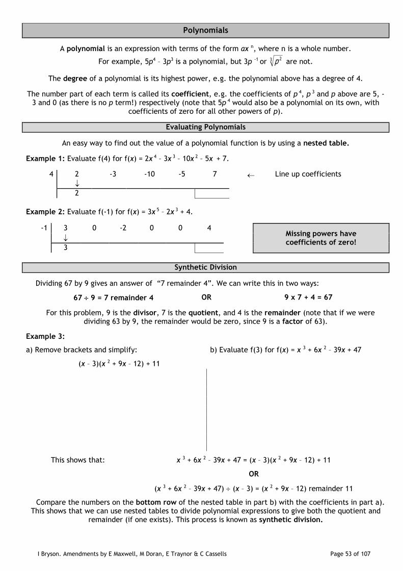
Example 10: The graph of the function y = x 3 – 7x 2 + 7x + 15 is shown. Find the coordinates of points A, B and C.
Finding a Function from its Graph
This uses exactly the same system as that for quadratic graphs, but with more brackets (see page 19).
Remember: tangents to the x – axis have repeated roots!
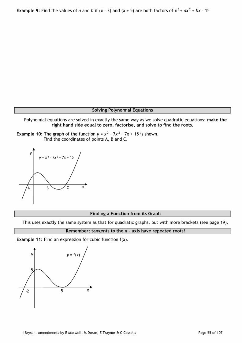
Example 11: Find an expression for cubic function f(x).
A B C
y = x 3 – 7x 2 + 7x + 15
x
y
-2 5
5
x
y = f(x) y
I Bryson. Amendments by E Maxwell, M Doran, E Traynor & C Cassells Page 56 of 107
Sketching Polynomial Functions
Example 12: a) Find the x – and y – intercepts of the graph of y = x 4 – 6x 3 + 13x 2 – 12x + 4.
b) Find the position and nature of the stationary points of y = x 4 – 6x 3 + 13x 2 – 12x + 4.
c) Hence, sketch and annotate the graph of y = x 4 – 6x 3 + 13x 2 – 12x + 4.

I Bryson. Amendments by E Maxwell, M Doran, E Traynor & C Cassells Page 57 of 107
Trigonometry: Addition Formulae and Equations
What you must know from National 5!!!
Sine Graph
Cosine Graph
We can use the above graphs to find the values of:
sin0 0
sin90 1
sin180 0
sin270 1
sin360 0
cos 0 1
cos 90 0
cos180 1
cos 270 0
cos 360 1
We can use these graphs to solve the following:
sin 0
0 360
0 ,180 ,360
x
x
x
sin 1
0 360
270
x
x
x
sin 1
0 360
90
x
x
x
cos 0
0 360
90 ,270
x
x
x
cos 1
0 360
270
x
x
x
cos 1
0 360
0 ,360
x
x
x
Remember , this means that:
sin 160° would be +
cos 200° would be –
tan 200° would be +
sin 320° would be – and so on...
y
x 0 90 180 270 360
-1
1
y = sinx° y = cosx°
y
x 0 90 180 270 360
-1
1
All + sin +
cos + tan +
0°
90°
180°
270°
360°
I Bryson. Amendments by E Maxwell, M Doran, E Traynor & C Cassells Page 58 of 107
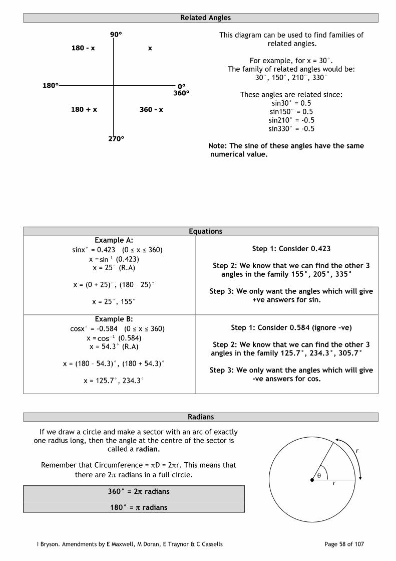
Related Angles
This diagram can be used to find families of
related angles.
For example, for x = 30°. The family of related angles would be:
30°, 150°, 210°, 330°
These angles are related since: sin30° = 0.5 sin150° = 0.5 sin210° = -0.5 sin330° = -0.5
Note: The sine of these angles have the same numerical value.
Equations
Example A:
sinx° = 0.423 (0 ≤ x ≤ 360)
x = 1sin (0.423) x = 25° (R.A)
x = (0 + 25)°, (180 – 25)°
x = 25°, 155°
Step 1: Consider 0.423
Step 2: We know that we can find the other 3
angles in the family 155°, 205°, 335°
Step 3: We only want the angles which will give +ve answers for sin.
Example B:
cosx° = -0.584 (0 ≤ x ≤ 360)
x = 1cos (0.584) x = 54.3° (R.A)
x = (180 – 54.3)°, (180 + 54.3)°
x = 125.7°, 234.3°
Step 1: Consider 0.584 (ignore –ve)
Step 2: We know that we can find the other 3 angles in the family 125.7°, 234.3°, 305.7°
Step 3: We only want the angles which will give
-ve answers for cos.
Radians
If we draw a circle and make a sector with an arc of exactly one radius long, then the angle at the centre of the sector is
called a radian.
Remember that Circumference = D = 2r. This means that
there are 2 radians in a full circle.
360° = 2 radians
180° = radians
r
r
x 180 - x
360 - x 180 + x
0°
90°
180°
270°
360°
I Bryson. Amendments by E Maxwell, M Doran, E Traynor & C Cassells Page 59 of 107
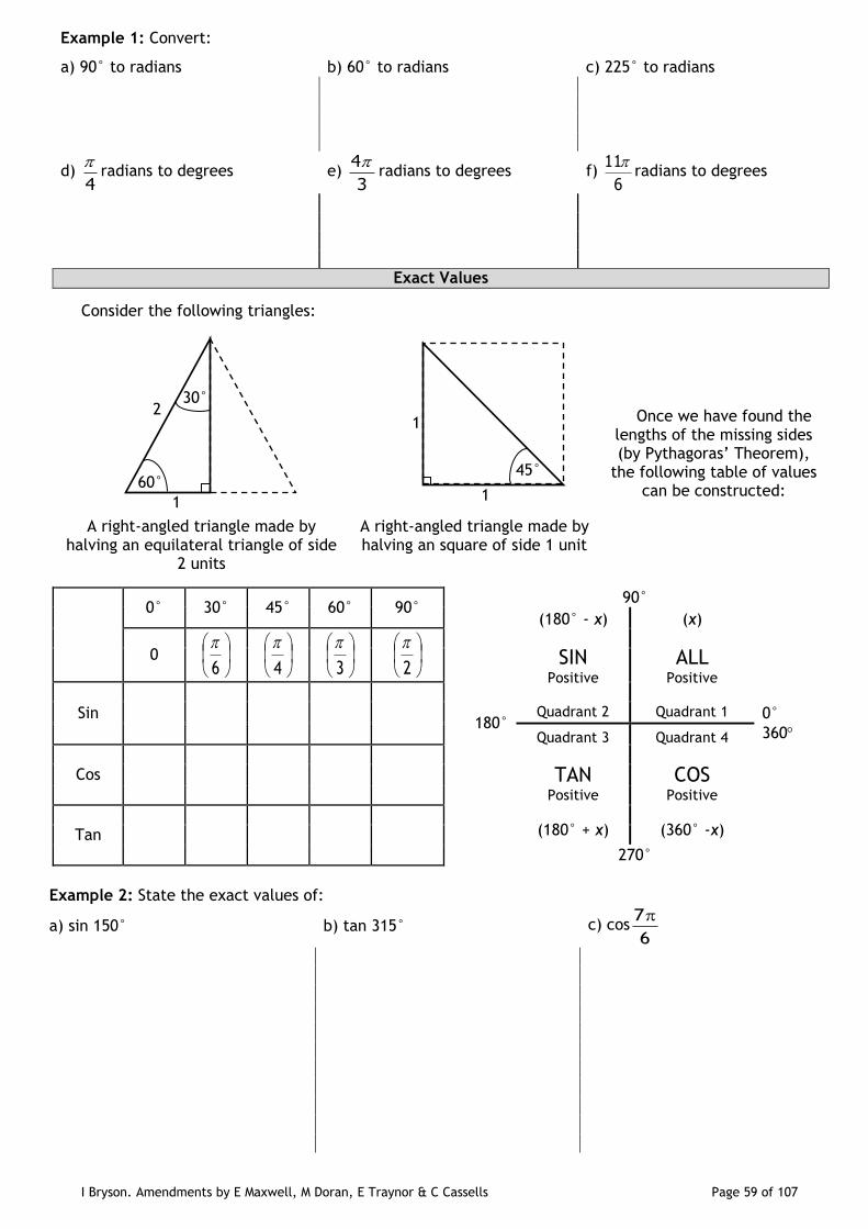
Example 1: Convert:
a) 90° to radians b) 60° to radians c) 225° to radians
d) 4
radians to degrees e)
3
4radians to degrees f)
6
11radians to degrees
Exact Values
Consider the following triangles:
Once we have found the lengths of the missing sides (by Pythagoras’ Theorem),
the following table of values can be constructed:
A right-angled triangle made by halving an equilateral triangle of side
2 units
A right-angled triangle made by halving an square of side 1 unit
0° 30° 45° 60° 90°
90°
(180° - x)
SIN Positive
Quadrant 2
(x)
ALL Positive
Quadrant 1
0
6
4
3
2
Sin
180° 0°
360 Quadrant 3
TAN Positive
(180° + x)
Quadrant 4
COS Positive
(360° -x)
Cos
Tan
270°
Example 2: State the exact values of:
a) sin 150° b) tan 315° c) cos6
7
1
2
60°
30°
45°
1
1
I Bryson. Amendments by E Maxwell, M Doran, E Traynor & C Cassells Page 60 of 107
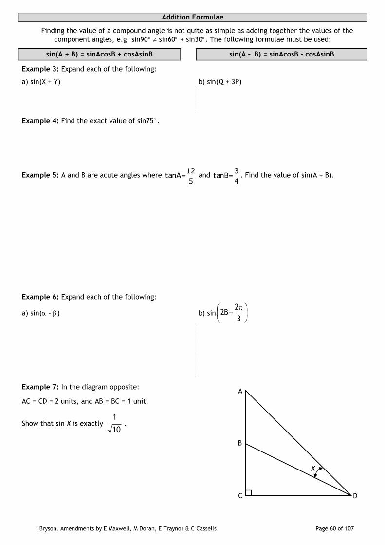
Addition Formulae
Finding the value of a compound angle is not quite as simple as adding together the values of the
component angles, e.g. sin90 sin60 + sin30. The following formulae must be used:
sin(A + B) = sinAcosB + cosAsinB sin(A – B) = sinAcosB - cosAsinB
Example 3: Expand each of the following:
a) sin(X + Y) b) sin(Q + 3P)
Example 4: Find the exact value of sin75°.
Example 5: A and B are acute angles where 5
12tanA and
4
3tanB . Find the value of sin(A + B).
Example 6: Expand each of the following:
a) sin( - ) b) sin
3
22B
Example 7: In the diagram opposite:
AC = CD = 2 units, and AB = BC = 1 unit.
Show that sin X is exactly 10
1.
X
A
D C
B
I Bryson. Amendments by E Maxwell, M Doran, E Traynor & C Cassells Page 61 of 107
cos(A + B) and cos (A – B)
cos(A + B) = cosAcosB - sinAsinB cos(A - B) = cosAcosB + sinAsinB
Example 8: Expand the following:
a) cos(X – Y) b) cos(X + 315)
Example 9:
a) Show that 1243
b) Hence find the exact value of cos
12
To summarise:
sin sin cos cos sinA B A B A B
cos cos cos sin sinA B A B A B
I Bryson. Amendments by E Maxwell, M Doran, E Traynor & C Cassells Page 62 of 107
Trigonometric Identities
NOTE: these are important formulae which are not provided in the exam paper formula sheets!
sintan
cos
xx
x
sin2x + cos2x = 1
Note that due to the second formula, we can also say that:
cos2x = 1 – sin2x AND sin2x = 1 – cos2x
To prove that an identity is true, we need to show that the expression on the left hand side of the equals sign can be changed into the expression on the right hand side.
Example 10: Prove that:
a) 4 4 2 2cos sin cos sin b) sin4
tan3 tancos cos3
c) 21 2sin 1
tantan sin cos
xx
x x x

I Bryson. Amendments by E Maxwell, M Doran, E Traynor & C Cassells Page 63 of 107
Double Angle Formulae
sin2A = sin(A + A) cos2A = cos(A + A)
=
=
Since cos2x = 1 – sin2x and sin2x = 1 – cos2x, we can further expand the formula for cos2A:
cos2A = cos2A – sin2A cos2A = cos2A – sin2A
=
=
To summarise:
sin2A = 2sinAcosA
= cos2A – sin2A
cos2A = 2cos2A - 1 = 1 – 2sin2A
Example 11: Express the following using double angle formulae:
a) sin2X b) sin6Y
c) cos2X (sine version) d) cos8H (cosine version)
e) sin5Q f) cos (cos and sin version)

I Bryson. Amendments by E Maxwell, M Doran, E Traynor & C Cassells Page 64 of 107
Example 12: 2
sin13
, where is an acute angle. Find the exact values of:
a) sin(2) b) cos(2)
Example 13: Prove that sin2
tan1 cos2
xx
x
Solving Complex Trig Equations
Trig equations can also often involve (i) powers of sin, cos or tan, and (ii) multiple and/or compound angles.
Example 14: Solve 4cos2x – 3 = 0 for 0 x 2

I Bryson. Amendments by E Maxwell, M Doran, E Traynor & C Cassells Page 65 of 107
Trig equations can also be written in forms which resemble quadratic equations: to solve these, treat them as such, and solve by factorisation.
Example 15: Solve 6sin2x – sinx – 2 = 0 for 0 x 360
If the equation contains a multiple angle term, solve as normal (paying close attention to the range of values of x ).
Example 16: Solve 3 tan 2 135 1x for 0 x 360
To solve trig equations with combinations of double- and single-angle angle terms:
Rewrite the double angle term using the formulae on Page 59
Factorise
Solve each factor for x
When the term is cos2X, the version of the double angle formula we use depends on the other terms in the equation: use 2cos2x – 1 if the other term is cosx ; 1 – 2sin2x if the other term is sinx.
Example 17: Solve sin2x – 2sinx = 0, 0 x 360
I Bryson. Amendments by E Maxwell, M Doran, E Traynor & C Cassells Page 66 of 107
Example 18: Solve 2cos2x – 7cosx = 0, 0 x 2
Formulae for cos2x and sin2x
Rearranging the formulae for cos2x allows us to obtain the following formulae for cos2x and sin2x
2 11 2
2 cos cosx x
sin cosx x 2 11 2
2
Example 19: Express each of the following without a squared term:
a) cos2θ b) sin23X c) sin2(
𝑥
2)
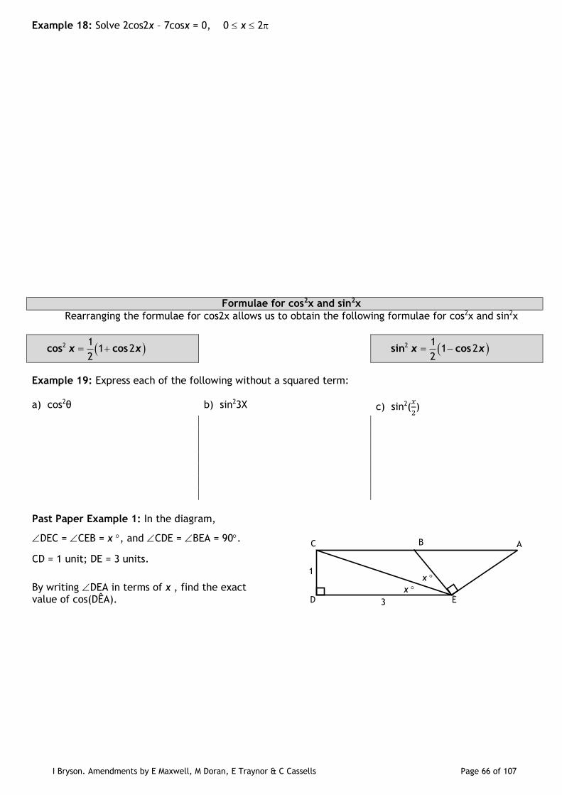
Past Paper Example 1: In the diagram,
DEC = CEB = x , and CDE = BEA = 90.
CD = 1 unit; DE = 3 units.
By writing DEA in terms of x , find the exact value of cos(DÊA).
A B C
D E
1
3
x
x
I Bryson. Amendments by E Maxwell, M Doran, E Traynor & C Cassells Page 67 of 107
Past Paper Example 2: Find the points of intersection of the graphs of y = 3cos2x + 2 and
y = 1 – cosx in the interval 0 x 360.
Past Paper Example 3: Solve algebraically the equation
sin2x = 2 cos2 x for 0 x 2
I Bryson. Amendments by E Maxwell, M Doran, E Traynor & C Cassells Page 68 of 107
Calculus 3: Further Calculus
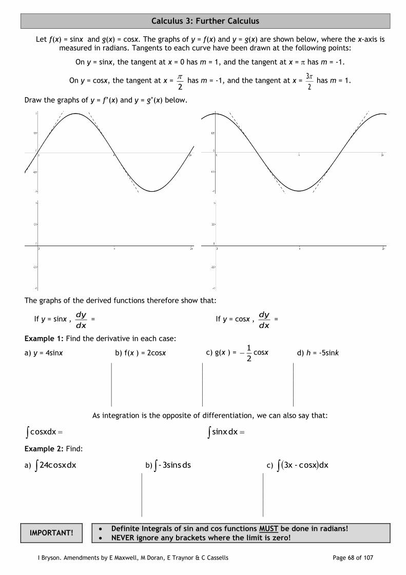
Let f(x) = sinx and g(x) = cosx. The graphs of y = f(x) and y = g(x) are shown below, where the x-axis is measured in radians. Tangents to each curve have been drawn at the following points:
On y = sinx, the tangent at x = 0 has m = 1, and the tangent at x = has m = -1.
On y = cosx, the tangent at x = 2
has m = -1, and the tangent at x =
2
3 has m = 1.
Draw the graphs of y = f’(x) and y = g’(x) below.
The graphs of the derived functions therefore show that:
If y = sinx , dx
dy = If y = cosx ,
dx
dy =
Example 1: Find the derivative in each case:
a) y = 4sinx b) f(x ) = 2cosx c) g(x ) = 2
1 cosx d) h = -5sink
As integration is the opposite of differentiation, we can also say that:
dxcosx dxsinx
Example 2: Find:
a) dx24cosx b) ds3sins- c) dxcosx -3x
IMPORTANT! Definite Integrals of sin and cos functions MUST be done in radians!
NEVER ignore any brackets where the limit is zero!
I Bryson. Amendments by E Maxwell, M Doran, E Traynor & C Cassells Page 69 of 107
Example 3: Evaluate:
a) π
2
0sinx dx b)
π4
0(sinx-cosx)dx
c) 3
02cos dxx
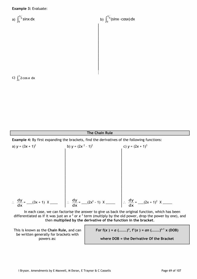
The Chain Rule
Example 4: By first expanding the brackets, find the derivatives of the following functions:
a) y = (3x + 1)2 b) y = (2x 2 – 1)2 c) y = (2x + 1)3
dx
dy= ___(3x + 1) X ____
dx
dy= ___(2x2 - 1) X _____
dx
dy= ___(2x + 1)2 X _____
In each case, we can factorise the answer to give us back the original function, which has been differentiated as if it was just an x 2 or x 3 term (multiply by the old power, drop the power by one), and
then multiplied by the derivative of the function in the bracket.
This is known as the Chain Rule, and can be written generally for brackets with
powers as:
For f(x ) = a (………)n, f’(x ) = an (………)n-1 x (DOB)
where DOB = the Derivative Of the Bracket
I Bryson. Amendments by E Maxwell, M Doran, E Traynor & C Cassells Page 70 of 107
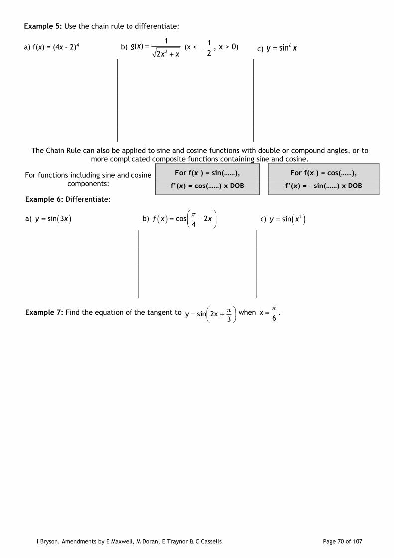
Example 5: Use the chain rule to differentiate:
a) f(x) = (4x – 2)4 b) 2
1( )
2g x
x x
(x <
2
1 , x > 0) c)
2siny x
The Chain Rule can also be applied to sine and cosine functions with double or compound angles, or to more complicated composite functions containing sine and cosine.
For functions including sine and cosine components:
For f(x ) = sin(……), For f(x ) = cos(……),
f’(x) = cos(……) x DOB f’(x) = - sin(……) x DOB
Example 6: Differentiate:
a) sin 3y x b) cos 24
f x x
c) 2siny x
Example 7: Find the equation of the tangent to
32xsiny when
6x
.
I Bryson. Amendments by E Maxwell, M Doran, E Traynor & C Cassells Page 71 of 107
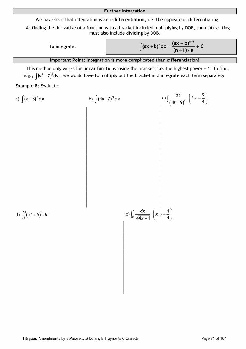
Further Integration
We have seen that integration is anti-differentiation, i.e. the opposite of differentiating.
As finding the derivative of a function with a bracket included multiplying by DOB, then integrating must also include dividing by DOB.
To integrate: Ca1)(n
b) (ax dxb)(ax
1nn
Important Point: Integration is more complicated than differentiation!
This method only works for linear functions inside the bracket, i.e. the highest power = 1. To find,
e.g., dg7g23 , we would have to multiply out the bracket and integrate each term separately.
Example 8: Evaluate:
a) dx3)(x 3 b) dx7)-(4x 9
c)
24 9
dt
t
9
4t
d) 2 3
12 5t dt e)
6
0
1
44 1
dxx
x
I Bryson. Amendments by E Maxwell, M Doran, E Traynor & C Cassells Page 72 of 107
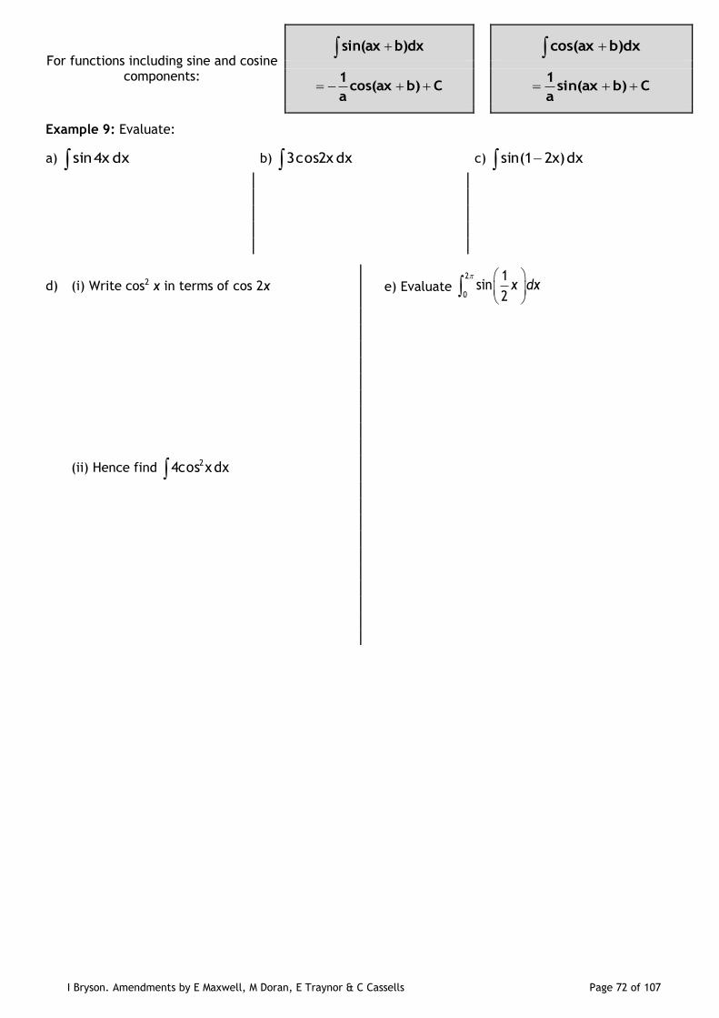
For functions including sine and cosine components:
b)dxsin(ax b)dxcos(ax
Cb)cos(axa
1 Cb)sin(ax
a
1
Example 9: Evaluate:
a) dx4xsin b) dx2xcos3 c) dx2x)(1sin
d) (i) Write cos2 x in terms of cos 2x e) Evaluate 2
0
1sin
2x dx
(ii) Hence find dxx4cos2
I Bryson. Amendments by E Maxwell, M Doran, E Traynor & C Cassells Page 73 of 107
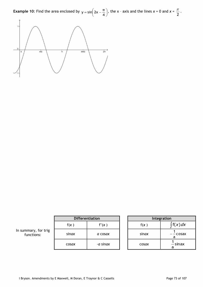
Example 10: Find the area enclosed by
4
π2xsiny , the x – axis and the lines x = 0 and x =
2
.
In summary, for trig functions:
Differentiation Integration
f(x ) f’(x ) f(x ) dxx )f(
sinax a cosax sinax cosaxa
1
cosax -a sinax cosax sinaxa
1
I Bryson. Amendments by E Maxwell, M Doran, E Traynor & C Cassells Page 74 of 107
Uses of Calculus in Real Life Situations
In the same way that geometry is the study of shape, calculus is the study of how functions change. This means that wherever a system can be described mathematically using a function, calculus can be used to find the ideal conditions (as we have seen using optimisation) or to use the rate of change at a
given time to find the total change (using integration).
As a result, calculus is used throughout the sciences: in Physics (Newton’s Laws of Motion, Einstein’s Theory of Relativity), Chemistry (reaction rates, radioactive decay), Biology (modelling changes in
population), Medicine (using the decay of drugs in the bloodstream to determine dosages), Economics (finding the maximum profit), Engineering (maximising the strength of a building whilst using the
minimum of material, working out the curved path of a rocket in space) and more.
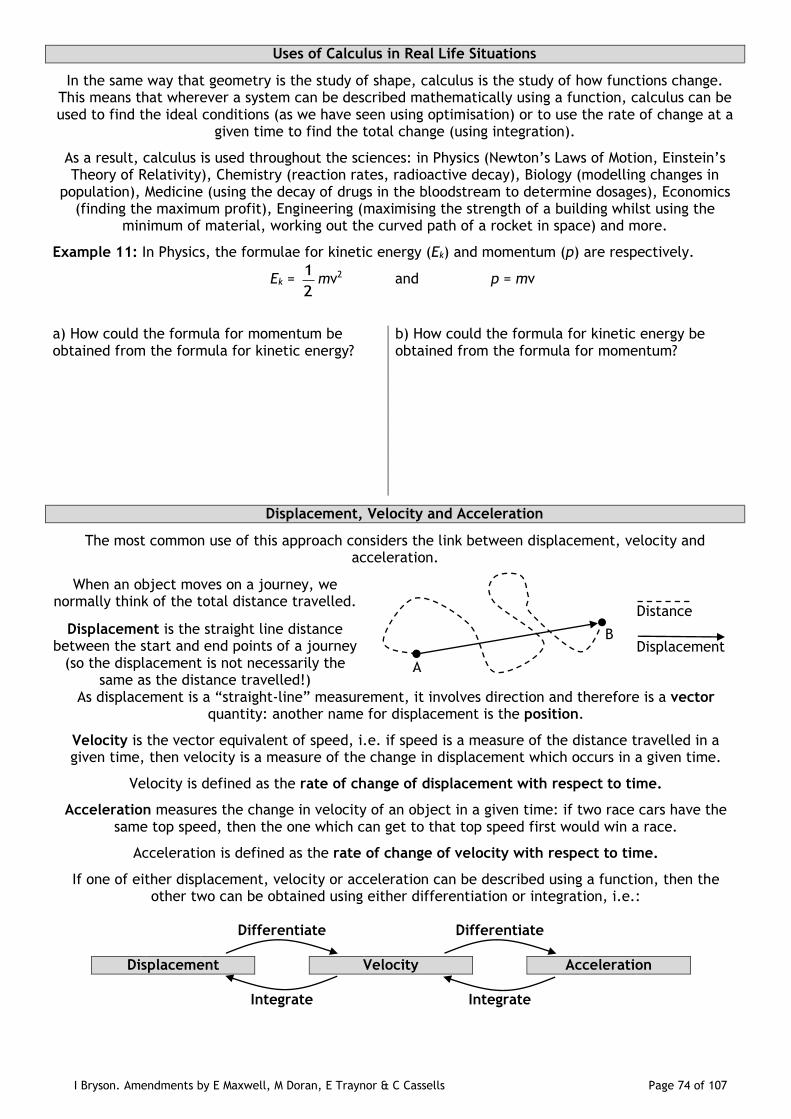
Example 11: In Physics, the formulae for kinetic energy (Ek) and momentum (p) are respectively.
Ek = 2
1mv2 and p = mv
a) How could the formula for momentum be obtained from the formula for kinetic energy?
b) How could the formula for kinetic energy be obtained from the formula for momentum?
Displacement, Velocity and Acceleration
The most common use of this approach considers the link between displacement, velocity and acceleration.
When an object moves on a journey, we normally think of the total distance travelled.
Displacement is the straight line distance between the start and end points of a journey
(so the displacement is not necessarily the same as the distance travelled!)
As displacement is a “straight-line” measurement, it involves direction and therefore is a vector quantity: another name for displacement is the position.
Velocity is the vector equivalent of speed, i.e. if speed is a measure of the distance travelled in a given time, then velocity is a measure of the change in displacement which occurs in a given time.
Velocity is defined as the rate of change of displacement with respect to time.
Acceleration measures the change in velocity of an object in a given time: if two race cars have the same top speed, then the one which can get to that top speed first would win a race.
Acceleration is defined as the rate of change of velocity with respect to time.
If one of either displacement, velocity or acceleration can be described using a function, then the other two can be obtained using either differentiation or integration, i.e.:
Differentiate Differentiate
Displacement Velocity Acceleration
Integrate Integrate
A
B
Distance
Displacement
I Bryson. Amendments by E Maxwell, M Doran, E Traynor & C Cassells Page 75 of 107
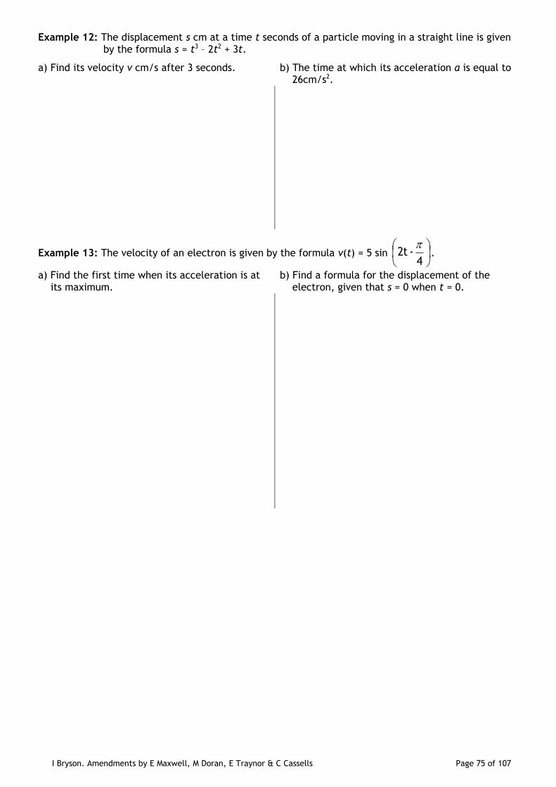
Example 12: The displacement s cm at a time t seconds of a particle moving in a straight line is given by the formula s = t3 – 2t2 + 3t.
a) Find its velocity v cm/s after 3 seconds. b) The time at which its acceleration a is equal to 26cm/s2.
Example 13: The velocity of an electron is given by the formula v(t) = 5 sin
4-2t
.
a) Find the first time when its acceleration is at its maximum.
b) Find a formula for the displacement of the electron, given that s = 0 when t = 0.
I Bryson. Amendments by E Maxwell, M Doran, E Traynor & C Cassells Page 76 of 107
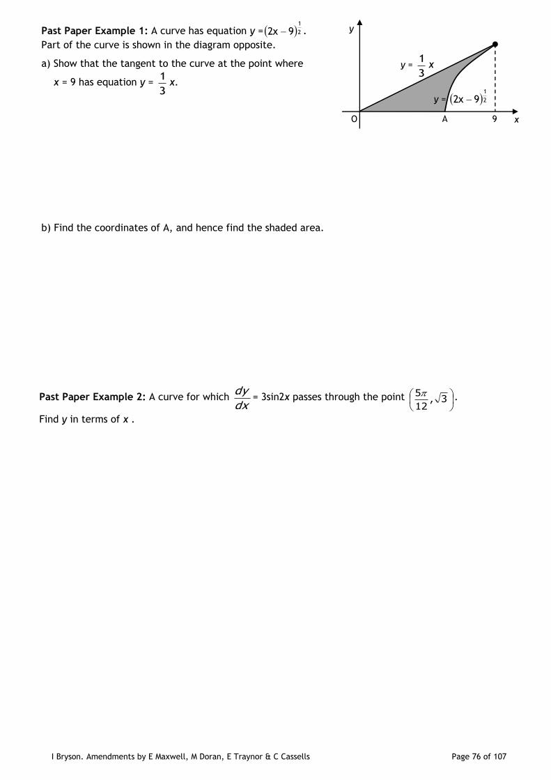
Past Paper Example 1: A curve has equation y = 2
1
92x .
Part of the curve is shown in the diagram opposite.
a) Show that the tangent to the curve at the point where
x = 9 has equation y = 3
1x.
b) Find the coordinates of A, and hence find the shaded area.
Past Paper Example 2: A curve for which dx
dy= 3sin2x passes through the point
3,
12
5 .
Find y in terms of x .
y
x O A 9
y = 2
1
92x
y = 3
1x
I Bryson. Amendments by E Maxwell, M Doran, E Traynor & C Cassells Page 77 of 107
Past Paper Example 3: Find the values of x for which the function f(x) = 2x + 3 + 4
18
x, x 4, is
increasing.
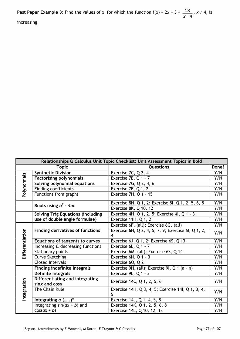
Relationships & Calculus Unit Topic Checklist: Unit Assessment Topics in Bold
Topic Questions Done?
Poly
nom
ials
Synthetic Division Exercise 7C, Q 2, 4 Y/N
Factorising polynomials Exercise 7E, Q 1 – 7 Y/N
Solving polynomial equations Exercise 7G, Q 2, 4, 6 Y/N
Finding coefficients Exercise 7F, Q 1, 2 Y/N
Functions from graphs Exercise 7H, Q 1 – 15 Y/N
Roots using b2 – 4ac Exercise 8H, Q 1, 2; Exercise 8I, Q 1, 2, 5, 6, 8 Y/N
Exercise 8K, Q 10, 12 Y/N
Solving Trig Equations (including use of double angle formulae)
Exercise 4H, Q 1, 2, 5; Exercise 4I, Q 1 – 3 Y/N
Exercise 11H, Q 1, 2 Y/N
Dif
fere
nti
ati
on
Finding derivatives of functions
Exercise 6F, (all); Exercise 6G, (all) Y/N
Exercise 6H, Q 2, 4, 5, 7, 9; Exercise 6I, Q 1, 2, 4
Y/N
Equations of tangents to curves Exercise 6J, Q 1, 2; Exercise 6S, Q 13 Y/N
Increasing & decreasing functions Exercise 6L, Q 1 - 7 Y/N
Stationary points Exercise 6M, (all); Exercise 6S, Q 14 Y/N
Curve Sketching Exercise 6N, Q 1 – 3 Y/N
Closed Intervals Exercise 6O, Q 2 Y/N
Inte
gra
tion
Finding indefinite integrals Exercise 9H, (all); Exercise 9I, Q 1 (a – n) Y/N
Definite Integrals Exercise 9L, Q 1 – 3 Y/N
Differentiating and integrating sinx and cosx
Exercise 14C, Q 1, 2, 5, 6 Y/N
The Chain Rule Exercise 14H, Q 3, 4, 5; Exercise 14I, Q 1, 3, 4, 5
Y/N
Integrating a (…..)n Exercise 14J, Q 1, 4, 5, 8 Y/N
Integrating sin(ax + b) and cos(ax + b)
Exercise 14K, Q 1, 2, 5, 6, 8 Y/N
Exercise 14L, Q 10, 12, 13 Y/N
I Bryson. Amendments by E Maxwell, M Doran, E Traynor & C Cassells Page 78 of 107
Vectors
Revision from National 5
A measurement which only describes the magnitude (i.e. size) of the object is called a scalar quantity, e.g. Glasgow is 11 miles from Airdrie. A vector is a quantity with magnitude and direction, e.g. Glasgow
is 11 miles from Airdrie on a bearing of 270°.
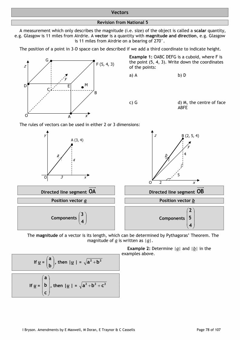
The position of a point in 3-D space can be described if we add a third coordinate to indicate height.
Example 1: OABC DEFG is a cuboid, where F is the point (5, 4, 3). Write down the coordinates of the points:
a) A b) D
c) G d) M, the centre of face ABFE
The rules of vectors can be used in either 2 or 3 dimensions:
Directed line segment OA Directed line segment OB
Position vector a Position vector b
Components
4
3 Components
4
5
2
The magnitude of a vector is its length, which can be determined by Pythagoras’ Theorem. The magnitude of a is written as |a|.
Example 2: Determine |a| and |b| in the examples above.
If u =
b
a, then |u | =
22 ba
If u =
c
b
a
, then |u | = 222 cba
x
y
z
O A
B C
E D
F (5, 4, 3) G
M
A (3, 4)
x
y
O 3
4
a
x
y
z
O
B (2, 5, 4)
b
2
5
4
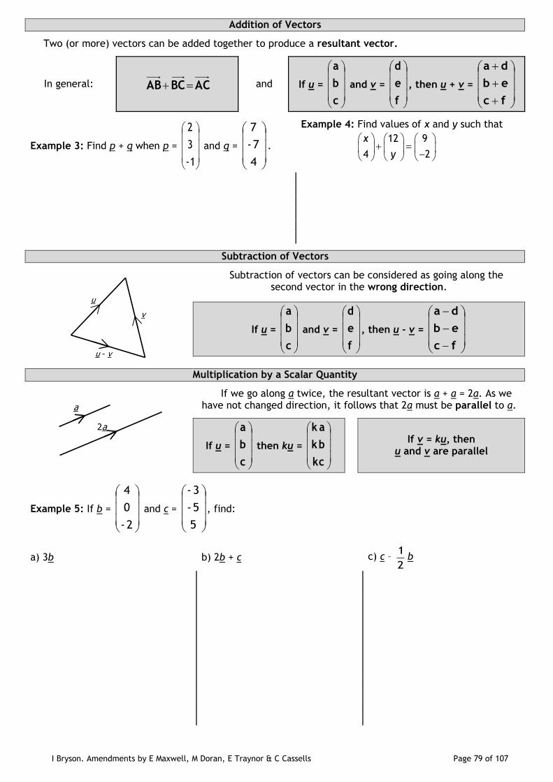
I Bryson. Amendments by E Maxwell, M Doran, E Traynor & C Cassells Page 79 of 107
Addition of Vectors
Two (or more) vectors can be added together to produce a resultant vector.
In general: ACBCAB and If u =
c
b
a
and v =
f
e
d
, then u + v =
fc
eb
da
Example 3: Find p + q when p =
1-
3
2
and q =
4
7-
7
.
Example 4: Find values of x and y such that
12 9
4 2
x
y
Subtraction of Vectors
Subtraction of vectors can be considered as going along the second vector in the wrong direction.
If u =
c
b
a
and v =
f
e
d
, then u - v =
fc
eb
da
Multiplication by a Scalar Quantity
If we go along a twice, the resultant vector is a + a = 2a. As we have not changed direction, it follows that 2a must be parallel to a.
If u =
c
b
a
then ku =
kc
bk
ak
If v = ku, then
u and v are parallel
Example 5: If b =
2-
0
4
and c =
5
5-
3-
, find:
a) 3b b) 2b + c c) c – 2
1b
u
v
u - v
a
2a
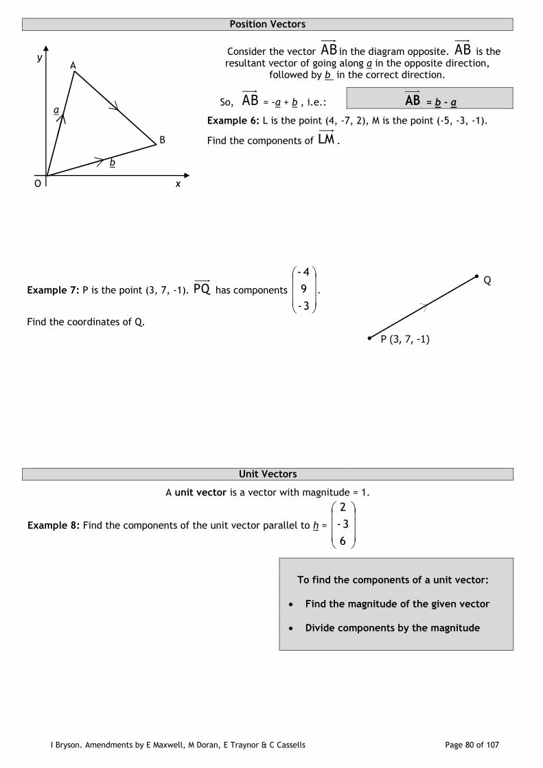
I Bryson. Amendments by E Maxwell, M Doran, E Traynor & C Cassells Page 80 of 107
Position Vectors
Consider the vector AB in the diagram opposite. AB is the resultant vector of going along a in the opposite direction,
followed by b in the correct direction.
So, AB = -a + b , i.e.: AB = b - a
Example 6: L is the point (4, -7, 2), M is the point (-5, -3, -1).
Find the components of LM .
Example 7: P is the point (3, 7, -1). PQ has components
3-
9
4-
.
Find the coordinates of Q.
Unit Vectors
A unit vector is a vector with magnitude = 1.
Example 8: Find the components of the unit vector parallel to h =
6
3-
2
To find the components of a unit vector:
Find the magnitude of the given vector
Divide components by the magnitude
a
b
A
B
O x
y
P (3, 7, -1)
Q
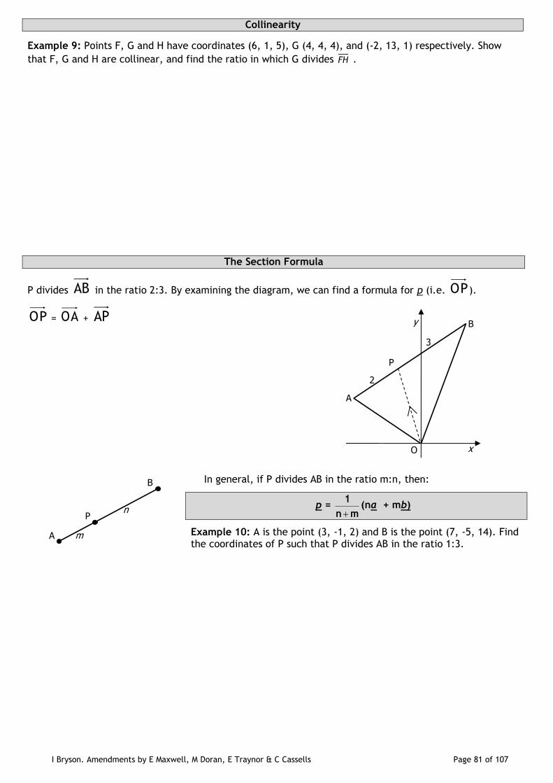
I Bryson. Amendments by E Maxwell, M Doran, E Traynor & C Cassells Page 81 of 107
Collinearity
Example 9: Points F, G and H have coordinates (6, 1, 5), G (4, 4, 4), and (-2, 13, 1) respectively. Show
that F, G and H are collinear, and find the ratio in which G divides FH .
The Section Formula
P divides AB in the ratio 2:3. By examining the diagram, we can find a formula for p (i.e. OP).
OP = OA + AP
In general, if P divides AB in the ratio m:n, then:
p = mn
1
(na + mb)
Example 10: A is the point (3, -1, 2) and B is the point (7, -5, 14). Find the coordinates of P such that P divides AB in the ratio 1:3.
x
y
O
A
B
P
2
3
A
P
B
m
n

I Bryson. Amendments by E Maxwell, M Doran, E Traynor & C Cassells Page 82 of 107
Vectors in 3D can also be described in terms of the three unit vectors i =
0
0
1
, j =
0
1
0
, and k =
1
0
0
,
which are parallel to the x, y, and z axes respectively.
Example 11: u = 3i + 2j - 6k, v = -i + 5j.
a) Express u + v in component form b) Find | u + v |
The Scalar Product (Angle Form)
The scalar product is the result of a type of multiplication of two vectors to give a scalar quantity. (i.e. a number with no directional component)
For vectors a and b , the scalar product (or dot product) is given as:
. cosa b a b Note: a and b point away from the vertex
0 ≤ ≤ 180°
Example 12: Find the scalar product in each case below, where a = 6 and b = 10.
a) b) c)
a
b
35°
a
b
a
b 103°
40°
a
b

I Bryson. Amendments by E Maxwell, M Doran, E Traynor & C Cassells Page 83 of 107
The Scalar Product (Component Form)
We can use the formula below to find the scalar product when we have been given the component forms of the two vectors but not the angle in between them.
If a =
3
2
1
a
a
a
and b =
3
2
1
b
b
b
, then a . b = a1b1 + a2b2 + a3b3
Example 13: a = i + 2j + 2k , and b = 2i + 3j - 6k . Evaluate a . b
Example 14: A is the point (1, 2, 3), B is the point (6, 5, 4) and C is the point (-1, -2, -6).
Evaluate .AB BC
Perpendicular Vectors
A special case of the scalar product occurs when we have
perpendicular vectors i.e. when θ = 90: a.b = |a||b| cos90
= |a||b| x 0 = 0
If a.b = 0, then a and b are perpendicular
Example 15: P, Q and R are the points (1, 1, 2), (-1, -1, 0) and (3, -4, -1) respectively. Find the
components of QP and QR , and hence show that the vectors are perpendicular.
I Bryson. Amendments by E Maxwell, M Doran, E Traynor & C Cassells Page 84 of 107
The Angle Between Two Vectors
We can rearrange the angle form of the scalar product to give ba
b.aθcos .
More specifically: BCBA
BC.BAABCcos
If the question gives you three points, you MUST find the components of the vectors pointing
AWAY from the vertex first!
Example 16: 2 2a i j k and 2 3 6b i j k . Find the angle between a and b .
Example 17: A is the point (1, 2, 3), B (6, 5, 4), and C (-1, -2, -6). Calculate ABC.
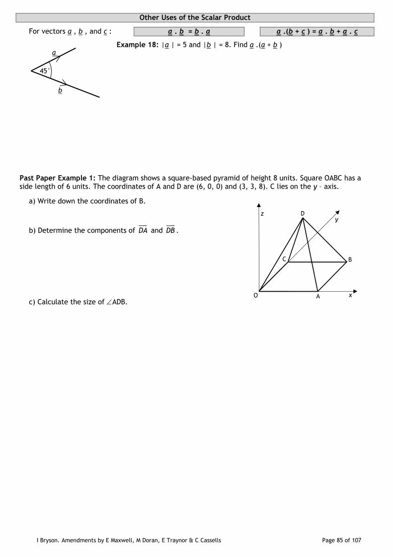
I Bryson. Amendments by E Maxwell, M Doran, E Traynor & C Cassells Page 85 of 107
Other Uses of the Scalar Product
For vectors a , b , and c : a . b = b . a a .(b + c ) = a . b + a . c
Example 18: |a | = 5 and |b | = 8. Find a .(a + b )
Past Paper Example 1: The diagram shows a square-based pyramid of height 8 units. Square OABC has a side length of 6 units. The coordinates of A and D are (6, 0, 0) and (3, 3, 8). C lies on the y – axis.
a) Write down the coordinates of B.
b) Determine the components of DA and DB .
c) Calculate the size of ADB.
45°
a
b
D
C B
A O x
y z

I Bryson. Amendments by E Maxwell, M Doran, E Traynor & C Cassells Page 86 of 107
Past Paper Example 2:
a) Show that the points A (-7, -8, 1), T (3, 2, 5) and B (18, 17, 11) are collinear and state the ratio in which T divides AB.
b) The point C lies on the x-axis.
If TB and TC are perpendicular, find the coordinates of C.
Past Paper Example 3: PQRSTU is a regular hexagon of side 2 units. PQ , QR and RS represent the vectors
a , b and c respectively. Find the value of a b c
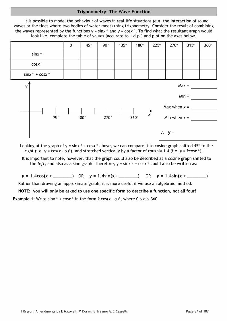
I Bryson. Amendments by E Maxwell, M Doran, E Traynor & C Cassells Page 87 of 107
Trigonometry: The Wave Function
It is possible to model the behaviour of waves in real-life situations (e.g. the interaction of sound waves or the tides where two bodies of water meet) using trigonometry. Consider the result of combining
the waves represented by the functions y = sinx and y = cosx . To find what the resultant graph would look like, complete the table of values (accurate to 1 d.p.) and plot on the axes below.
0 45 90 135 180 225 270 315 360
sinx
cosx
sinx + cosx
Max =
Min =
Max when x =
Min when x =
y =
Looking at the graph of y = sinx + cosx above, we can compare it to cosine graph shifted 45 to the
right (i.e. y = cos(x - )), and stretched vertically by a factor of roughly 1.4 (i.e. y = kcosx ).
It is important to note, however, that the graph could also be described as a cosine graph shifted to
the left, and also as a sine graph! Therefore, y = sinx + cosx could also be written as:
y = 1.4cos(x + _______) OR y = 1.4sin(x - _______) OR y = 1.4sin(x + _______)
Rather than drawing an approximate graph, it is more useful if we use an algebraic method.
NOTE: you will only be asked to use one specific form to describe a function, not all four!
Example 1: Write sinx + cosx in the form k cos(x – ), where 0 360.
90° 180° 270° 360° x
y
I Bryson. Amendments by E Maxwell, M Doran, E Traynor & C Cassells Page 88 of 107
This technique can also include the difference between waves and to include double (or higher) angles, but only when the angles of both the sin and cos term are the same (i.e. 2cos2x + 5sin2x can
be written as a wave function, but 2cos2x + 5sin3x could not).
Example 2: Write sinx –3cosx in the form k cos(x - ), where 0 2
Example 3: Write 12cosx – 5sinx in the form k sin(x - ), where 0 360
Example 4: Write 2sin2 - cos2 in the form k sin(2 + ), where 0 2
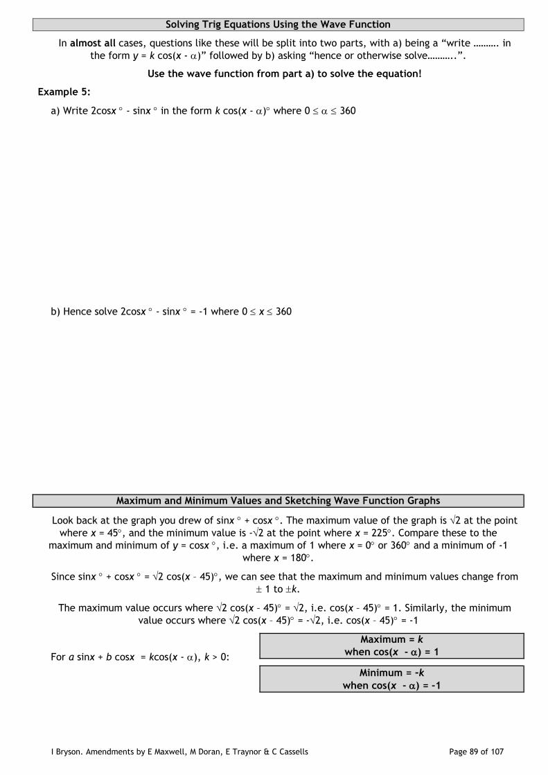
I Bryson. Amendments by E Maxwell, M Doran, E Traynor & C Cassells Page 89 of 107
Solving Trig Equations Using the Wave Function
In almost all cases, questions like these will be split into two parts, with a) being a “write ………. in
the form y = k cos(x - )” followed by b) asking “hence or otherwise solve………..”.
Use the wave function from part a) to solve the equation!
Example 5:
a) Write 2cosx - sinx in the form k cos(x - ) where 0 360
b) Hence solve 2cosx - sinx = -1 where 0 x 360
Maximum and Minimum Values and Sketching Wave Function Graphs
Look back at the graph you drew of sinx + cosx . The maximum value of the graph is 2 at the point
where x = 45, and the minimum value is -2 at the point where x = 225. Compare these to the
maximum and minimum of y = cosx , i.e. a maximum of 1 where x = 0 or 360 and a minimum of -1
where x = 180.
Since sinx + cosx = 2 cos(x – 45), we can see that the maximum and minimum values change from
1 to k.
The maximum value occurs where 2 cos(x – 45) = 2, i.e. cos(x – 45) = 1. Similarly, the minimum
value occurs where 2 cos(x – 45) = -2, i.e. cos(x – 45) = -1
For a sinx + b cosx = kcos(x - ), k > 0:
Maximum = k
when cos(x - ) = 1
Minimum = -k
when cos(x - ) = -1

I Bryson. Amendments by E Maxwell, M Doran, E Traynor & C Cassells Page 90 of 107
Example 6:
a) Write 3sinx + cosx in the form k cos(x – )°, where 0 360°
b) Find algebraically for 0 x 360°:
(i) The maximum and minimum turning points of
y = 3sinx° + cosx° .
(ii) The points of intersection of
y = 3sinx° + cosx° with the coordinate axes.
c) Sketch and annotate the graph of y = 3sinx° + cosx° for 0 x 360°.
90° 180° 270° 360° x
y
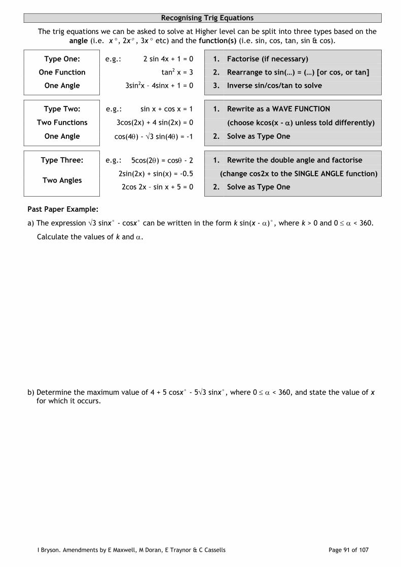
I Bryson. Amendments by E Maxwell, M Doran, E Traynor & C Cassells Page 91 of 107
Recognising Trig Equations
The trig equations we can be asked to solve at Higher level can be split into three types based on the
angle (i.e. x , 2x , 3x etc) and the function(s) (i.e. sin, cos, tan, sin & cos).
Type One: e.g.: 2 sin 4x + 1 = 0 1. Factorise (if necessary)
One Function tan2 x = 3 2. Rearrange to sin(…) = (…) [or cos, or tan]
One Angle 3sin2x – 4sinx + 1 = 0 3. Inverse sin/cos/tan to solve
Type Two: e.g.: sin x + cos x = 1 1. Rewrite as a WAVE FUNCTION
Two Functions 3cos(2x) + 4 sin(2x) = 0 (choose kcos(x - ) unless told differently)
One Angle cos(4) - 3 sin(4) = -1 2. Solve as Type One
Type Three: e.g.: 5cos(2) = cos - 2 1. Rewrite the double angle and factorise
Two Angles 2sin(2x) + sin(x) = -0.5 (change cos2x to the SINGLE ANGLE function)
2cos 2x – sin x + 5 = 0 2. Solve as Type One
Past Paper Example:
a) The expression 3 sinx° - cosx° can be written in the form k sin(x - )°, where k > 0 and 0 < 360.
Calculate the values of k and .
b) Determine the maximum value of 4 + 5 cosx° - 53 sinx°, where 0 < 360, and state the value of x for which it occurs.

I Bryson. Amendments by E Maxwell, M Doran, E Traynor & C Cassells Page 92 of 107
Inverse Functions
If a function links every number in the domain to only one number in the range, the function is called a one to one correspondence.
When function f(x) is a one to one correspondence from A to B, the function which maps from B back to A is called the inverse function,
written f -1(x).
For example, if f(x) = 2x, the inverse would be the function which “cancels out” multiplication by 2, i.e. f-1(x ) = ½x
Finding the Formula of an Inverse Function
We can find the formula for the inverse of a function through a process very similar to changing the subject of a formula.
Example 1: For each function shown find a formula for the inverse function.
a) f(x) = 2x + 5 b) g(x) = 2
1(x – 9)
c) p(x) = 3x 3 – 4 d) 3 17
4
xh x
x
If f(g(x)) = x , then f(x) and g(x) are inverse functions, so that
f(x) = g-1(x) AND g(x) = f-1(x)
Example 2: f(x) = 2x + 5 and g(x) = 2
5x . Show that g(x) = f-1(x)
A B
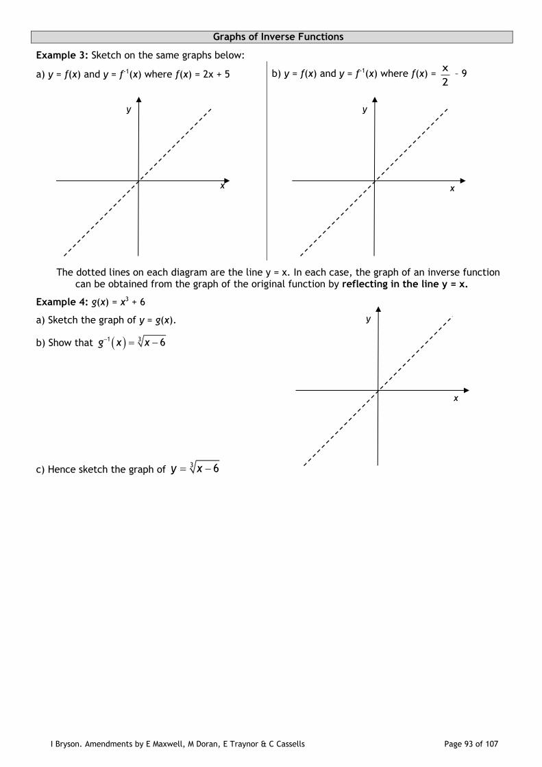
I Bryson. Amendments by E Maxwell, M Doran, E Traynor & C Cassells Page 93 of 107
Graphs of Inverse Functions
Example 3: Sketch on the same graphs below:
a) y = f(x) and y = f-1(x) where f(x) = 2x + 5 b) y = f(x) and y = f-1(x) where f(x) = 2
x – 9
The dotted lines on each diagram are the line y = x. In each case, the graph of an inverse function can be obtained from the graph of the original function by reflecting in the line y = x.
Example 4: g(x) = x3 + 6
a) Sketch the graph of y = g(x).
b) Show that 1 3 6g x x
c) Hence sketch the graph of 3 6y x
x
y
x
y
x
y
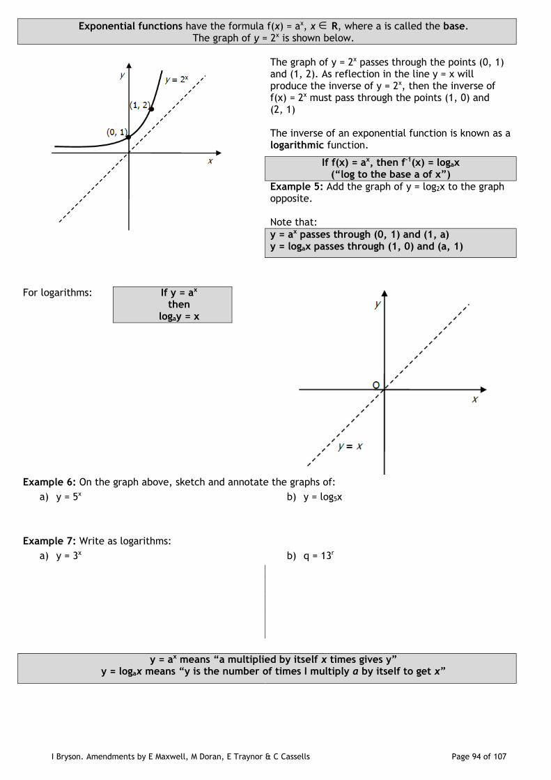
I Bryson. Amendments by E Maxwell, M Doran, E Traynor & C Cassells Page 94 of 107
Exponential functions have the formula f(x) = ax, x R, where a is called the base. The graph of y = 2x is shown below.
The graph of y = 2x passes through the points (0, 1) and (1, 2). As reflection in the line y = x will produce the inverse of y = 2x, then the inverse of f(x) = 2x must pass through the points (1, 0) and (2, 1) The inverse of an exponential function is known as a logarithmic function.
If f(x) = ax, then f-1(x) = logax (“log to the base a of x”)
Example 5: Add the graph of y = log2x to the graph opposite. Note that:
y = ax passes through (0, 1) and (1, a) y = logax passes through (1, 0) and (a, 1)
For logarithms: If y = ax then
logay = x
Example 6: On the graph above, sketch and annotate the graphs of:
a) y = 5x b) y = log5x
Example 7: Write as logarithms:
a) y = 3x b) q = 13r
y = ax means “a multiplied by itself x times gives y” y = logax means “y is the number of times I multiply a by itself to get x”
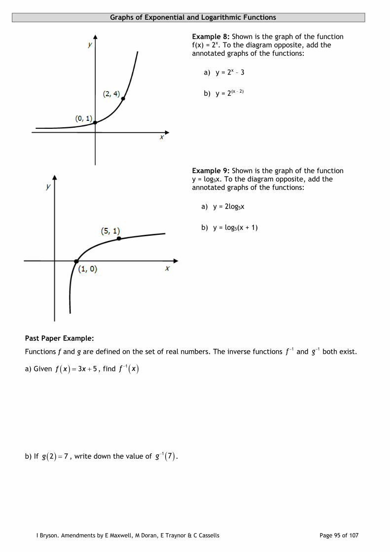
I Bryson. Amendments by E Maxwell, M Doran, E Traynor & C Cassells Page 95 of 107
Graphs of Exponential and Logarithmic Functions
Example 8: Shown is the graph of the function f(x) = 2x. To the diagram opposite, add the annotated graphs of the functions:
a) y = 2x – 3
b) y = 2(x – 2)
Example 9: Shown is the graph of the function y = log5x. To the diagram opposite, add the annotated graphs of the functions:
a) y = 2log5x
b) y = log5(x + 1)
Past Paper Example:
Functions f and g are defined on the set of real numbers. The inverse functions 1f and
1g both exist.
a) Given 3 5f x x , find 1f x
b) If 2 7g , write down the value of 1 7g.

I Bryson. Amendments by E Maxwell, M Doran, E Traynor & C Cassells Page 96 of 107
Exponential and Logarithmic Functions
Exponential functions are those with variable powers, e.g. y = a x. Their graphs take two forms:
When a > 1, the graph: When 0 < a < 1, the graph
is always increasing
is always positive
never cuts the x – axis
passes through (0, 1)
shows exponential growth
is always decreasing
is always positive
never cuts the x – axis
passes through (0, 1)
shows exponential decay
Exponential Functions as Models
Example 11: Ulanda’s population in 2016 was 100 million and it was growing at 6% per annum.
a) Find a formula Pn for the population in millions, n years later.
b) Estimate the population in the year 2026
Example 12: 8000 gallons of oil are lost in an oil spill in Blue Sky Bay. At the beginning of each week a filter plant removes 67% of the oil present.
a) Find a formula Gn for the amount of oil left in the bay after n weeks.
b) After how many complete weeks will there be less than 10 gallons left?
x
y
(0, 1)
x
y
(0, 1)
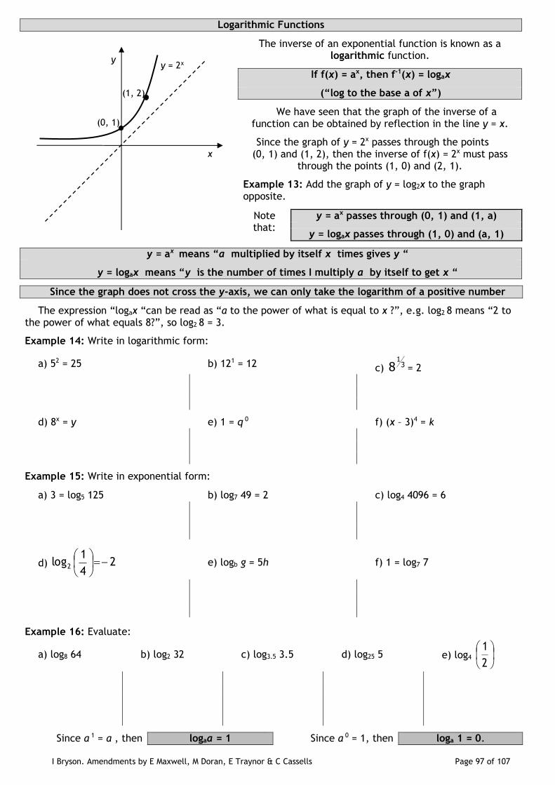
I Bryson. Amendments by E Maxwell, M Doran, E Traynor & C Cassells Page 97 of 107
Logarithmic Functions
The inverse of an exponential function is known as a logarithmic function.
If f(x) = ax, then f-1(x) = logax
(“log to the base a of x”)
We have seen that the graph of the inverse of a function can be obtained by reflection in the line y = x.
Since the graph of y = 2x passes through the points (0, 1) and (1, 2), then the inverse of f(x) = 2x must pass
through the points (1, 0) and (2, 1).
Example 13: Add the graph of y = log2x to the graph opposite.
Note that:
y = ax passes through (0, 1) and (1, a)
y = logax passes through (1, 0) and (a, 1)
y = ax means “a multiplied by itself x times gives y “
y = logax means “y is the number of times I multiply a by itself to get x “
Since the graph does not cross the y-axis, we can only take the logarithm of a positive number
The expression “logax “can be read as “a to the power of what is equal to x ?”, e.g. log2 8 means “2 to the power of what equals 8?”, so log2 8 = 3.
Example 14: Write in logarithmic form:
a) 52 = 25 b) 121 = 12 c) 31
8 = 2
d) 8x = y e) 1 = q 0 f) (x – 3)4 = k
Example 15: Write in exponential form:
a) 3 = log5 125 b) log7 49 = 2 c) log4 4096 = 6
d) 24
1log2
e) logb g = 5h f) 1 = log7 7
Example 16: Evaluate:
a) log8 64 b) log2 32 c) log3.5 3.5 d) log25 5 e) log4
2
1
Since a 1 = a , then logaa = 1 Since a 0 = 1, then loga 1 = 0.
(0, 1)
(1, 2)
x
y y = 2x
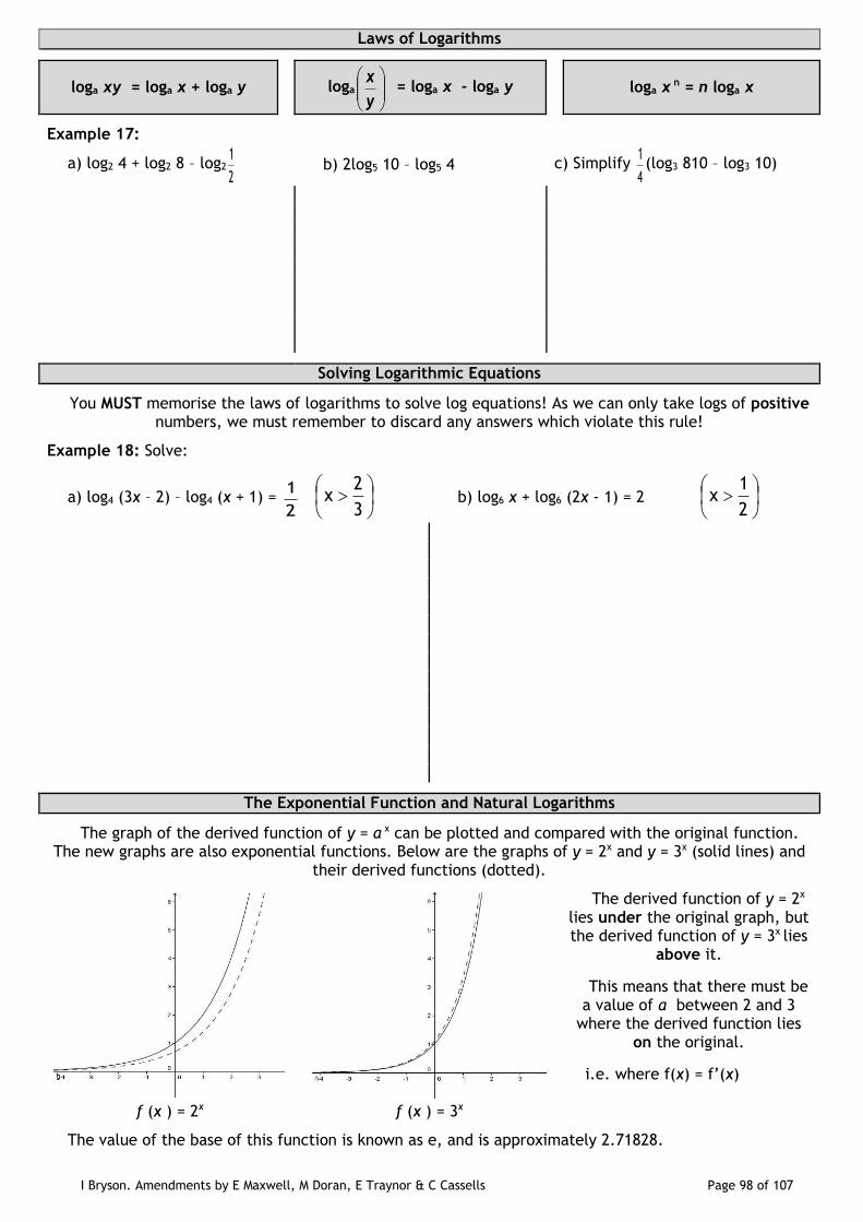
I Bryson. Amendments by E Maxwell, M Doran, E Traynor & C Cassells Page 98 of 107
Laws of Logarithms
loga xy = loga x + loga y loga
y
x = loga x - loga y loga x
n = n loga x
Example 17:
a) log2 4 + log2 8 – log2
2
1 b) 2log5 10 – log5 4 c) Simplify
4
1(log3 810 – log3 10)
Solving Logarithmic Equations
You MUST memorise the laws of logarithms to solve log equations! As we can only take logs of positive numbers, we must remember to discard any answers which violate this rule!
Example 18: Solve:
a) log4 (3x – 2) – log4 (x + 1) = 2
1
3
2x b) log6 x + log6 (2x - 1) = 2
2
1x
The Exponential Function and Natural Logarithms
The graph of the derived function of y = a x can be plotted and compared with the original function. The new graphs are also exponential functions. Below are the graphs of y = 2x and y = 3x (solid lines) and
their derived functions (dotted).
The derived function of y = 2x lies under the original graph, but the derived function of y = 3x lies
above it.
This means that there must be a value of a between 2 and 3
where the derived function lies on the original.
i.e. where f(x) = f’(x)
f (x ) = 2x f (x ) = 3x
The value of the base of this function is known as e, and is approximately 2.71828.
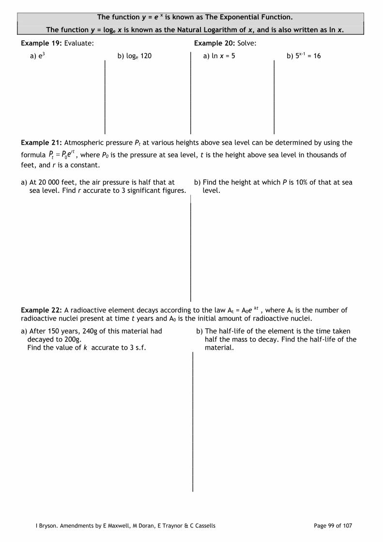
I Bryson. Amendments by E Maxwell, M Doran, E Traynor & C Cassells Page 99 of 107
The function y = e x is known as The Exponential Function.
The function y = loge x is known as the Natural Logarithm of x, and is also written as ln x.
Example 19: Evaluate: Example 20: Solve:
a) e3 b) loge 120 a) ln x = 5 b) 5x-1 = 16
Example 21: Atmospheric pressure Pt at various heights above sea level can be determined by using the
formula 0
rt
tP P e , where P0 is the pressure at sea level, t is the height above sea level in thousands of
feet, and r is a constant.
a) At 20 000 feet, the air pressure is half that at sea level. Find r accurate to 3 significant figures.
b) Find the height at which P is 10% of that at sea level.
Example 22: A radioactive element decays according to the law At = A0e kt , where At is the number of radioactive nuclei present at time t years and A0 is the initial amount of radioactive nuclei.
a) After 150 years, 240g of this material had decayed to 200g. Find the value of k accurate to 3 s.f.
b) The half-life of the element is the time taken half the mass to decay. Find the half-life of the material.
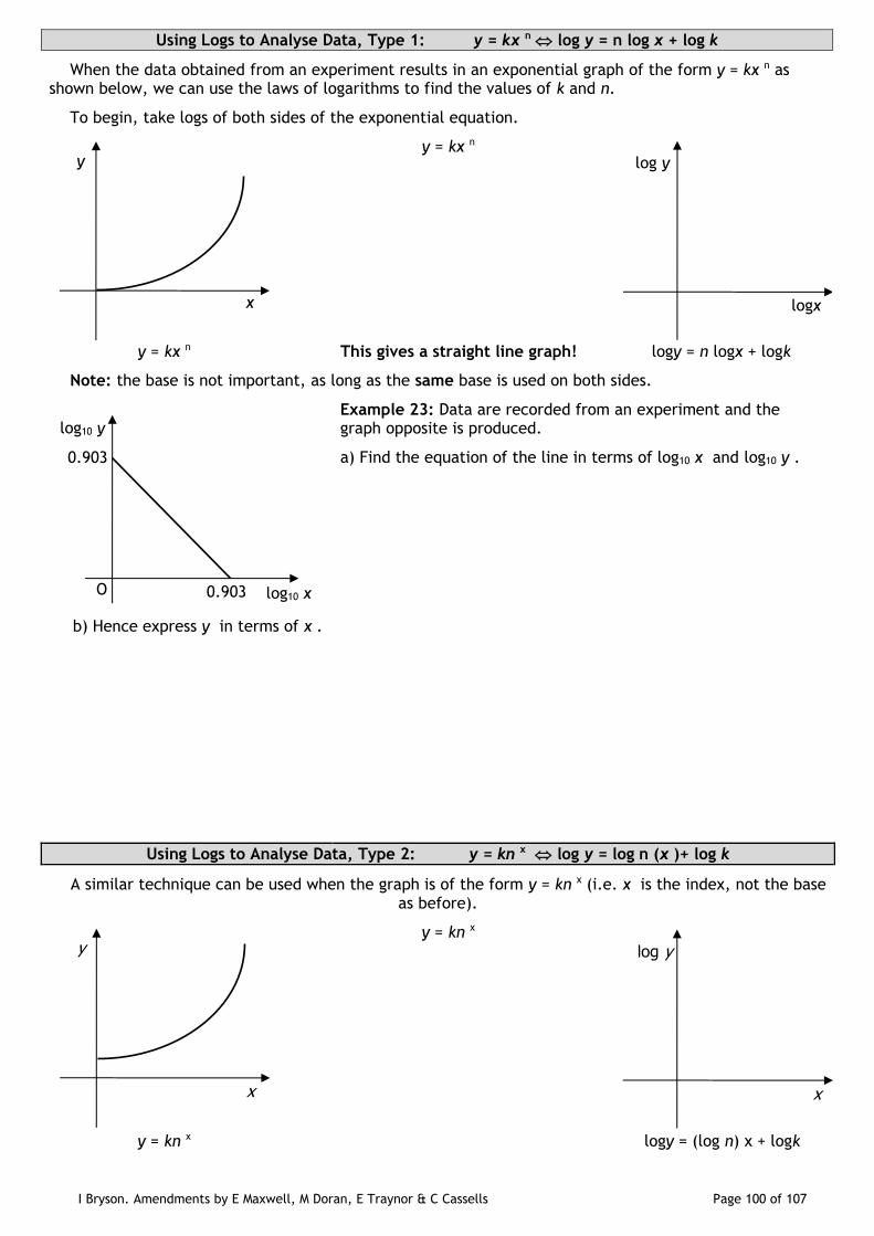
I Bryson. Amendments by E Maxwell, M Doran, E Traynor & C Cassells Page 100 of 107
Using Logs to Analyse Data, Type 1: y = kx n log y = n log x + log k
When the data obtained from an experiment results in an exponential graph of the form y = kx n as shown below, we can use the laws of logarithms to find the values of k and n.
To begin, take logs of both sides of the exponential equation.
y = kx n
y = kx n This gives a straight line graph! logy = n logx + logk
Note: the base is not important, as long as the same base is used on both sides.
Example 23: Data are recorded from an experiment and the graph opposite is produced.
a) Find the equation of the line in terms of log10 x and log10 y .
b) Hence express y in terms of x .
Using Logs to Analyse Data, Type 2: y = kn x log y = log n (x )+ log k
A similar technique can be used when the graph is of the form y = kn x (i.e. x is the index, not the base as before).
y = kn x
y = kn x logy = (log n) x + logk
x
y
logx
log y
0.903
0.903 log10 x
log10 y
O
x
y
x
log y
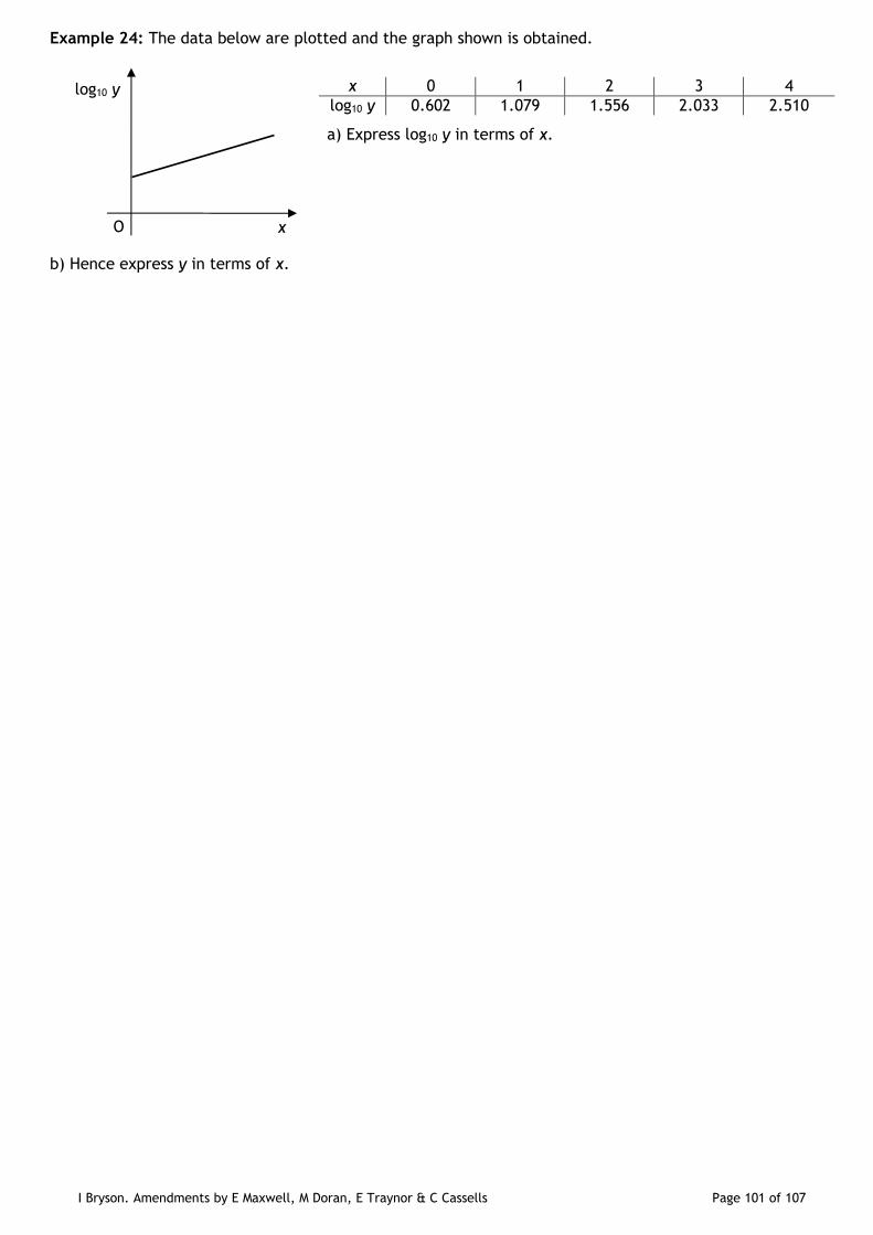
I Bryson. Amendments by E Maxwell, M Doran, E Traynor & C Cassells Page 101 of 107
Example 24: The data below are plotted and the graph shown is obtained.
x 0 1 2 3 4
log10 y 0.602 1.079 1.556 2.033 2.510
a) Express log10 y in terms of x.
b) Hence express y in terms of x.
x
log10 y
O
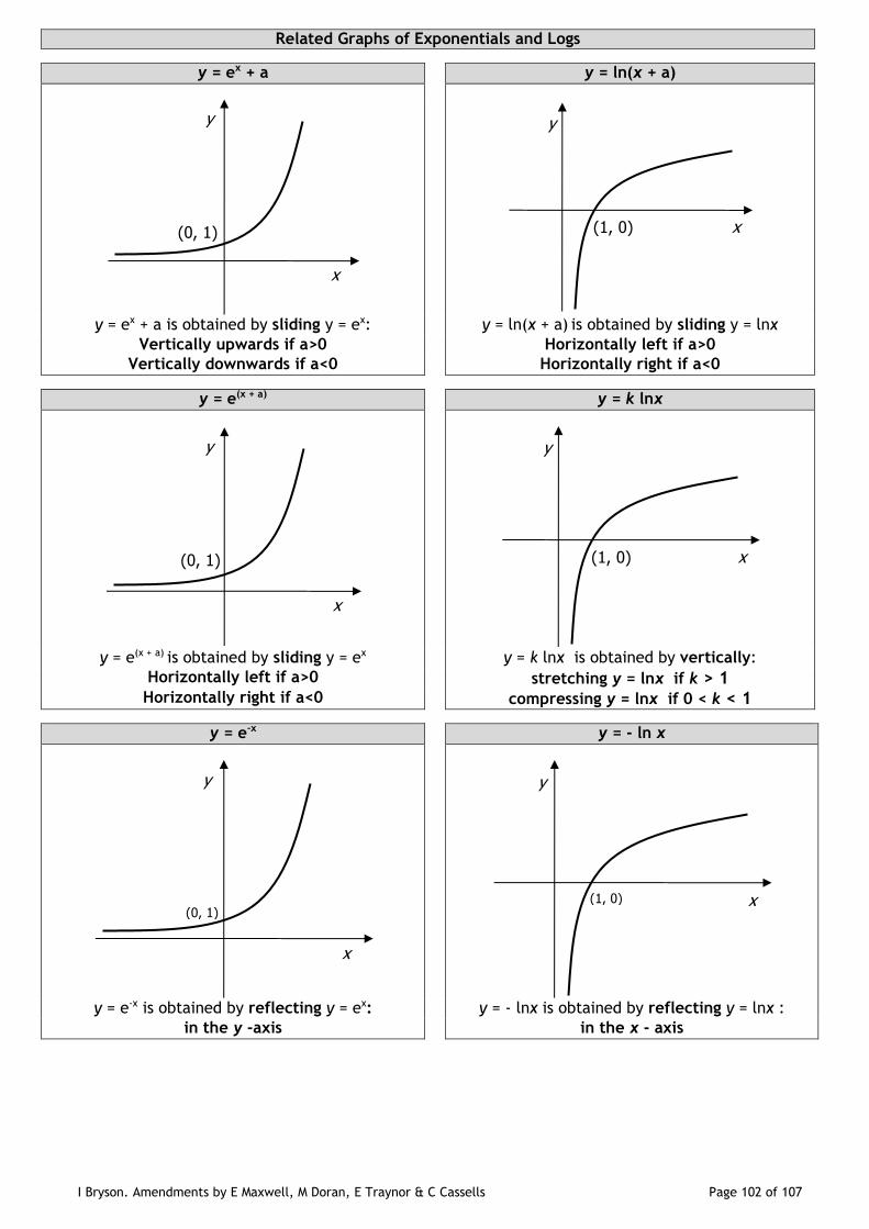
I Bryson. Amendments by E Maxwell, M Doran, E Traynor & C Cassells Page 102 of 107
Related Graphs of Exponentials and Logs
y = ex + a y = ln(x + a)
y = ex + a is obtained by sliding y = ex: y = ln(x + a) is obtained by sliding y = lnx
Vertically upwards if a>0 Horizontally left if a>0
Vertically downwards if a<0 Horizontally right if a<0
y = e(x + a) y = k lnx
y = e(x + a) is obtained by sliding y = ex y = k lnx is obtained by vertically:
Horizontally left if a>0 stretching y = lnx if k > 1 Horizontally right if a<0 compressing y = lnx if 0 < k < 1
y = e-x y = - ln x
y = e-x is obtained by reflecting y = ex: y = - lnx is obtained by reflecting y = lnx :
in the y -axis in the x - axis
x
y
(0, 1) x
y
(1, 0)
x
y
(0, 1) x
y
(1, 0)
x
y
(0, 1) x
y
(1, 0)
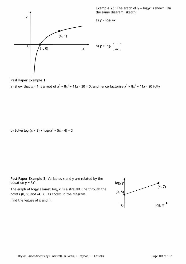
I Bryson. Amendments by E Maxwell, M Doran, E Traynor & C Cassells Page 103 of 107
Example 25: The graph of y = log4x is shown. On the same diagram, sketch:
a) y = log4 4x
b) y = log4
4x
1
Past Paper Example 1:
a) Show that x = 1 is a root of x3 + 8x2 + 11x – 20 = 0, and hence factorise x3 + 8x2 + 11x – 20 fully
b) Solve log2(x + 3) + log2(x2 + 5x – 4) = 3
Past Paper Example 2: Variables x and y are related by the equation y = kxn.
The graph of log2y against 2
log x is a straight line through the
points (0, 5) and (4, 7), as shown in the diagram.
Find the values of k and n.
x
y
(1, 0)
(4, 1)
O
(4, 7)
(0, 5)
log2 y
log2 x O
I Bryson. Amendments by E Maxwell, M Doran, E Traynor & C Cassells Page 104 of 107
Past Paper Example 3: The concentration of the pesticide Xpesto in soil is modelled by the equation:
P0 is the initial concentration
0
kt
tP P e where: Pt is the concentration at time t
t is the time, in days, after the application of the pesticide.
a) Once in the soil, the half-life of a pesticide is the time taken for its concentration to be reduced to one half of its initial value.
b) Eighty days after the initial application, what is the percentage decrease in Xpesto?
If the half-life of Xpesto is 25 days, find the value of k to 2 significant figures.
Past Paper Example 4: Simplify the expression
3log 2 2log 3e e
e e giving your answer in the form
log loge e
A B C , where A, B and C are whole
numbers.
Past Paper Example 5: Two variables x and y
satisfy the equation 3 4xy .
A graph is drawn of 10
log y against x. Show that its
equation will be of the form 10
log y Px Q , and
state the gradient and y-intercept of this line.
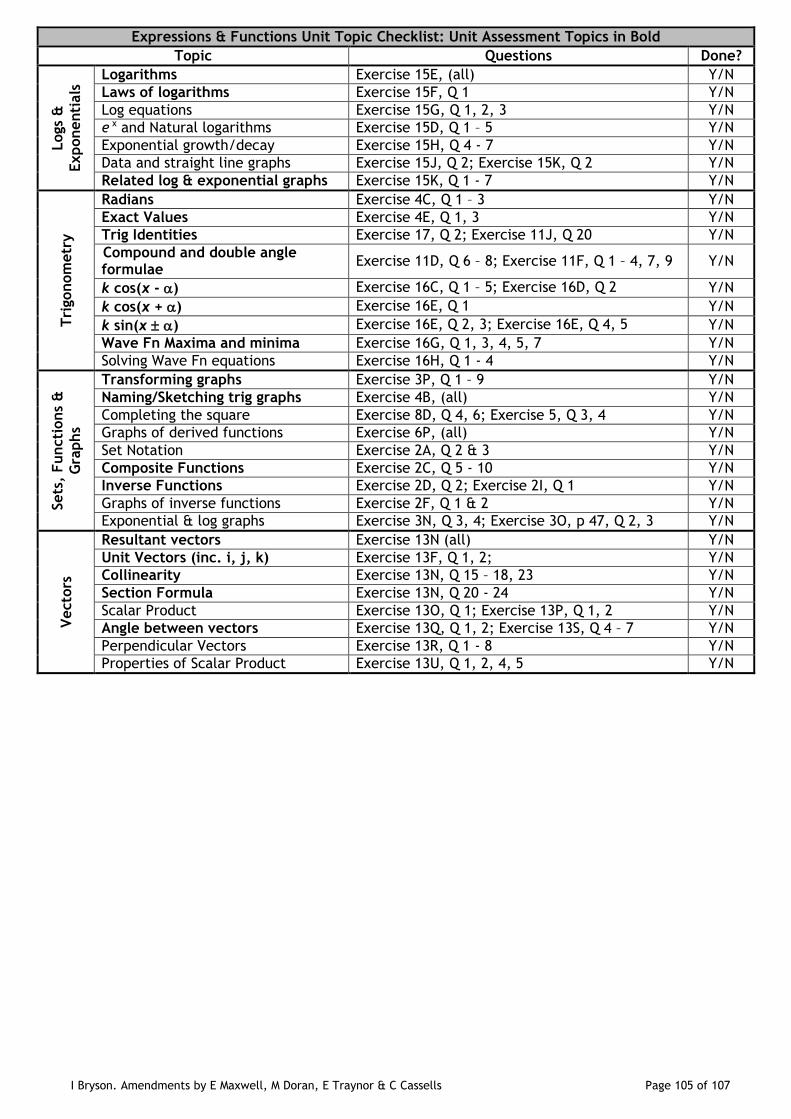
I Bryson. Amendments by E Maxwell, M Doran, E Traynor & C Cassells Page 105 of 107
Expressions & Functions Unit Topic Checklist: Unit Assessment Topics in Bold
Topic Questions Done? Logs
&
Exponenti
als
Logarithms Exercise 15E, (all) Y/N
Laws of logarithms Exercise 15F, Q 1 Y/N
Log equations Exercise 15G, Q 1, 2, 3 Y/N
e x and Natural logarithms Exercise 15D, Q 1 – 5 Y/N
Exponential growth/decay Exercise 15H, Q 4 - 7 Y/N
Data and straight line graphs Exercise 15J, Q 2; Exercise 15K, Q 2 Y/N
Related log & exponential graphs Exercise 15K, Q 1 - 7 Y/N
Tri
gonom
etr
y
Radians Exercise 4C, Q 1 – 3 Y/N
Exact Values Exercise 4E, Q 1, 3 Y/N
Trig Identities Exercise 17, Q 2; Exercise 11J, Q 20 Y/N
Compound and double angle formulae
Exercise 11D, Q 6 – 8; Exercise 11F, Q 1 – 4, 7, 9 Y/N
k cos(x - ) Exercise 16C, Q 1 – 5; Exercise 16D, Q 2 Y/N
k cos(x + ) Exercise 16E, Q 1 Y/N
k sin(x ) Exercise 16E, Q 2, 3; Exercise 16E, Q 4, 5 Y/N
Wave Fn Maxima and minima Exercise 16G, Q 1, 3, 4, 5, 7 Y/N
Solving Wave Fn equations Exercise 16H, Q 1 - 4 Y/N
Sets
, Functi
ons
&
Gra
phs
Transforming graphs Exercise 3P, Q 1 – 9 Y/N
Naming/Sketching trig graphs Exercise 4B, (all) Y/N
Completing the square Exercise 8D, Q 4, 6; Exercise 5, Q 3, 4 Y/N
Graphs of derived functions Exercise 6P, (all) Y/N
Set Notation Exercise 2A, Q 2 & 3 Y/N
Composite Functions Exercise 2C, Q 5 - 10 Y/N
Inverse Functions Exercise 2D, Q 2; Exercise 2I, Q 1 Y/N
Graphs of inverse functions Exercise 2F, Q 1 & 2 Y/N
Exponential & log graphs Exercise 3N, Q 3, 4; Exercise 3O, p 47, Q 2, 3 Y/N
Vecto
rs
Resultant vectors Exercise 13N (all) Y/N
Unit Vectors (inc. i, j, k) Exercise 13F, Q 1, 2; Y/N
Collinearity Exercise 13N, Q 15 – 18, 23 Y/N
Section Formula Exercise 13N, Q 20 - 24 Y/N
Scalar Product Exercise 13O, Q 1; Exercise 13P, Q 1, 2 Y/N
Angle between vectors Exercise 13Q, Q 1, 2; Exercise 13S, Q 4 – 7 Y/N
Perpendicular Vectors Exercise 13R, Q 1 - 8 Y/N
Properties of Scalar Product Exercise 13U, Q 1, 2, 4, 5 Y/N
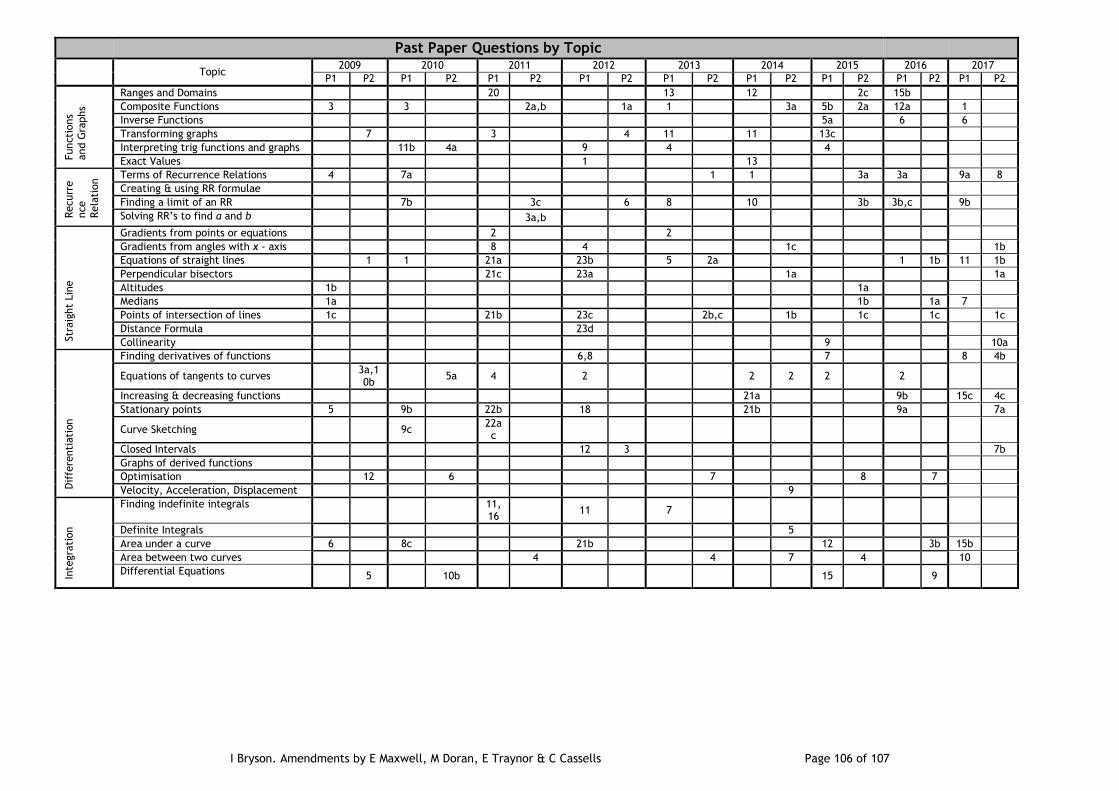
I Bryson. Amendments by E Maxwell, M Doran, E Traynor & C Cassells Page 106 of 107
Past Paper Questions by Topic
Topic 2009 2010 2011 2012 2013 2014 2015 2016 2017
P1 P2 P1 P2 P1 P2 P1 P2 P1 P2 P1 P2 P1 P2 P1 P2 P1 P2 Functi
ons
and G
raphs
Ranges and Domains 20 13 12 2c 15b
Composite Functions 3 3 2a,b 1a 1 3a 5b 2a 12a 1
Inverse Functions 5a 6 6
Transforming graphs 7 3 4 11 11 13c
Interpreting trig functions and graphs 11b 4a 9 4 4
Exact Values 1 13
Recurr
e
nce
Rela
tion Terms of Recurrence Relations 4 7a 1 1 3a 3a 9a 8
Creating & using RR formulae
Finding a limit of an RR 7b 3c 6 8 10 3b 3b,c 9b
Solving RR’s to find a and b 3a,b
Str
aig
ht
Lin
e
Gradients from points or equations 2 2
Gradients from angles with x - axis 8 4 1c 1b
Equations of straight lines 1 1 21a 23b 5 2a 1 1b 11 1b
Perpendicular bisectors 21c 23a 1a 1a
Altitudes 1b 1a
Medians 1a 1b 1a 7
Points of intersection of lines 1c 21b 23c 2b,c 1b 1c 1c 1c
Distance Formula 23d
Collinearity 9 10a
Dif
fere
nti
ati
on
Finding derivatives of functions 6,8 7 8 4b
Equations of tangents to curves 3a,10b
5a 4 2 2 2 2 2
Increasing & decreasing functions 21a 9b 15c 4c
Stationary points 5 9b 22b 18 21b 9a 7a
Curve Sketching 9c 22ac
Closed Intervals 12 3 7b
Graphs of derived functions
Optimisation 12 6 7 8 7
Velocity, Acceleration, Displacement 9
Inte
gra
tion
Finding indefinite integrals
11,16
11 7
Definite Integrals 5
Area under a curve 6 8c 21b 12 3b 15b
Area between two curves 4 4 7 4 10
Differential Equations 5 10b 15 9
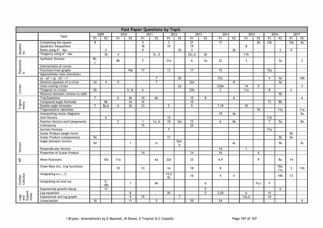
I Bryson. Amendments by E Maxwell, M Doran, E Traynor & C Cassells Page 107 of 107
Past Paper Questions by Topic
Topic 2009 2010 2011 2012 2013 2014 2015 2016 2017
P1 P2 P1 P2 P1 P2 P1 P2 P1 P2 P1 P2 P1 P2 P1 P2 P1 P2
Quadra
t
ics
Completing the square 8 5 3 21 17 2b 12b 15a 4a
Quadratic Inequations 18 19 19 8
Roots using b2 – 4ac 2 9 1b 3 3b 2 4
Tangency using b2 – 4ac 3b 4 2c, d 22c,d 3b 11b
Poly
nom
ia
ls
Synthetic Division 9b, c
8b 7 21a 6 3a 22 3 3a 2
Intersections of curves
Functions from graphs 10a 17 13 17 15 15a
Approximate roots (Iteration)
Cir
cle
s
(x – a)2 + (y – b)2 = r2 7 2b 23c 4 4a 10b
General equation of a circle 2a 4 5 7 22a 8 4a
Lines cutting circles 2a 23ab 14 5 3
Tangents to circles 2b 3, 5c 6 22b 2 11a 8 2
Distance between centres vs radii 4b
Tri
gono
metr
y
Trig Equations 7 6 4b 10 6b 15 8 6 6
Compound angle formulae 8b 2a 12 10 13 8b
Double angle formulae 7 8a,b 6 2b 23 5 9 7,18 10
Trigonometric identities 7b 11a 11a
Vecto
rs
Interpreting vector diagrams 19 4a 5a
Unit Vectors 6 15 11b
Position Vectors and Components 2 1 1a, b 10 5ai 12 6 4b 7 5a 5b
Collinearity 15 24
Section Formula 7 11a
Scalar Product (angle form) 5b
Scalar Product (components) 9a 17 5b 5a
Angle between vectors 9d 1 1c
5aii,b
4c 5b 5c
Perpendicular Vectors 14 1
Properties of Scalar Product 14 14 16 6
WF
Wave Functions 10a 11a 6a 22a 23 4,9 9 8a 14
Furt
her
Calc
ulu
s
Chain Rule (inc. trig functions) 10 13 16 18 8
10a, 11c
3 11b
Integrating a (…..)n
14,22b
16 5 5 10b 13
Integrating sin and cos
9, 10b
7 6b 6 7a,c 5
Logs
and
Expone
nti
als
Exponential growth/decay 11 9 6
Log equations 8 20 5 3,20 6 14
Exponential and log graphs 9 19 7 13a,b 10
Linearisation 10 11 5 20 24 9