1

HIGH STRAIN RATE COMPRESSION-SHEAR BEHAVIOR OF A SHEAR-THICKENING FLUID (STF)

Amanda S. Lim1, 2, Bazle A. Gama1 and John W. Gillespie Jr.1, 2, 3

1University of Delaware Center for Composite Materials (UD-CCM) 2Department of Materials Science and Engineering

3Department of Civil and Environmental Engineering University of Delaware, Newark, DE 19716

ABSTRACT

Fabrics impregnated with shear thickening fluids have attracted much attention recently for their behavior under impact loadings. Discontinuous shear thickening fluids experience a dramatic increase in viscosity when exposed to shear rates above a critical value; this is referred to as the ‘shear-thickened’ state. The behavior of the STF in this shear-thickened regime is not currently understood, despite many studies into the behavior of a STF prior to thickening. Due to the interest in the shear thickened state of discontinuous STFs for numerous applications, an understanding of the STF behavior in this state is critical. Towards this end, a novel testing technique has been proposed which utilizes current compression split-Hopkinson pressure bar (SHPB) methodologies in a dynamic squeeze flow experiment to induce shear to the STF at levels of strain rate that are not achievable in traditional rheometers. Once test parameters required for thickening are determined, the bar can be further used to apply an additional compressive force allowing the measurement of the compressive stress-strain response within the post-transition STF. Since the impedance of the STF is very low, aluminum bars are used in the experiments. Preliminary experiments show that the transmitted stress waves can be measured with sufficient accuracy. Detailed results and data reduction procedures will be presented. KEY WORDS: Applications – Military, Materials – Particulates /Fillers/Reinforcements, Test Methods/Test Standardization

1. INTRODUCTION Recently, the protective behavior of fabrics infused with shear-thickening fluid has attracted interest into the rheological behavior of an STF. The addition of STF to Nylon and Kevlar fabrics has been shown empirically to improve extremity protection through ballistic, spike, and stab testing (1-8). Currently, however, a fundamental understanding of STF mechanisms in a fabric during a ballistic event has not yet been achieved. Within the fabric, the STF is subjected to high stresses and is likely in its post-transition state. In a recent study into the behavior of short fiber reinforced STF under ballistic threats, the authors state that “the similarities between the squeeze flow and ballistic results indicate that the shearing and elongational flows during squeeze flow mimic some of the flow dynamics taking place during ballistic impact” (9). In order to fully understand the role of STF in fabric during a ballistic event, it is necessary to first fully characterize the behavior of a shear thickening fluid.

2

Typical strain rates produced by a rheometer range from 0-300 s-1. However, the strain rates which occur during fabric impact events can be an order of magnitude greater. Thus, the ideal characterization of a shear-thickening fluid would cover a very large range of shear/strain rates. An experimental procedure capable of achieving higher strain rates is necessary for full characterization of a STF. The following sections describe a modification of the split Hopkinson pressure bar (SHPB) experimental technique allowing for the dynamic squeeze flow testing of fluids. As the compressive force due to the incident bar causes the fluid to deform axially, the fluid will expand in the radial direction, thus inducing shear. The test parameters (bar material, striker bar velocity, pulse shaper, specimen thickness) can be adjusted to achieve shear rates required for a thickening response within the material. In addition, the SHPB is capable of imparting high stress levels that may be required to initiate failure of the STF in the post-transition state. While, shear thickening fluids have been characterized rheologically prior to stiffening (10 and 11), there is little knowledge of the fluid behavior in the post-transition state. Once the material has reached its post-transition state, the subsequent impacts will yield the stress-strain response of the thickened material providing strain rate dependent properties (e.g. stiffness, strength and strain to failure). Thus, the multiple impacts which occur during the SHPB test lend this technique an advantage over other (static) test methods.

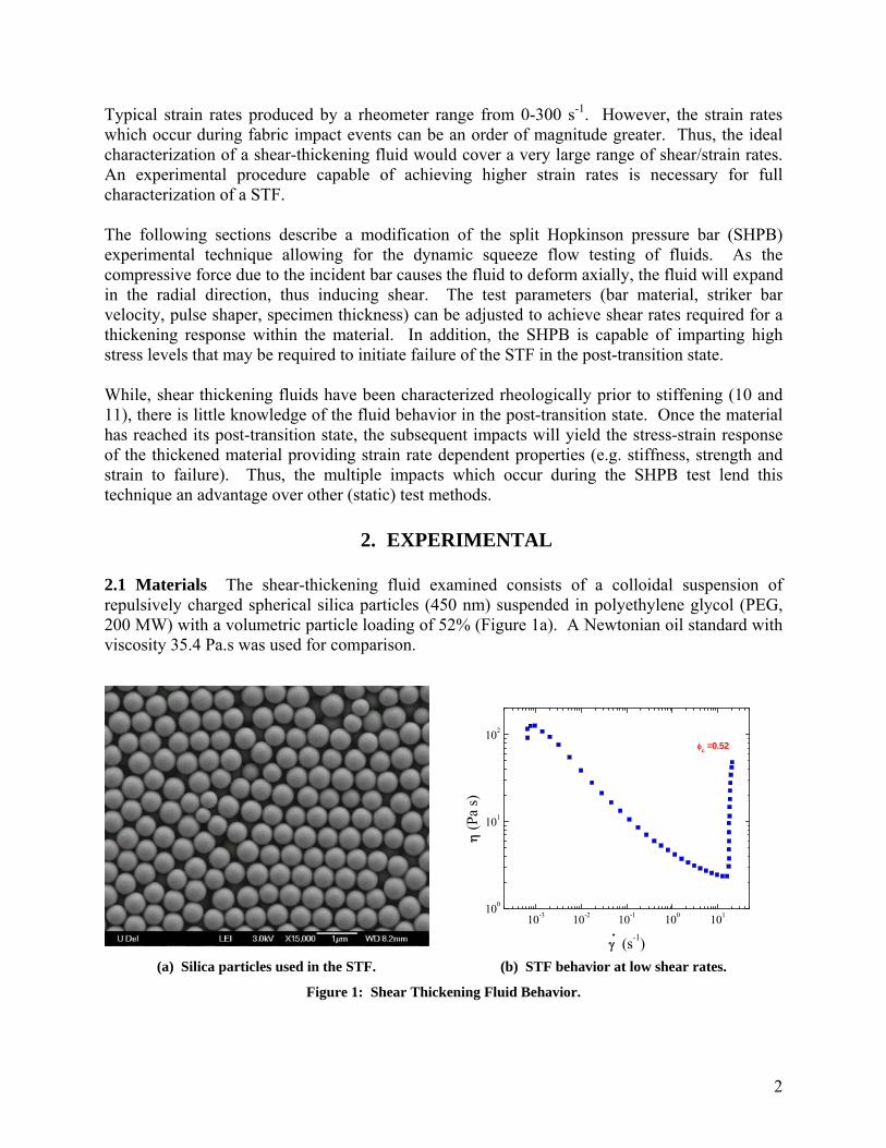
2. EXPERIMENTAL 2.1 Materials The shear-thickening fluid examined consists of a colloidal suspension of repulsively charged spherical silica particles (450 nm) suspended in polyethylene glycol (PEG, 200 MW) with a volumetric particle loading of 52% (Figure 1a). A Newtonian oil standard with viscosity 35.4 Pa.s was used for comparison.

10-3 10-2 10-1 100 101100

101

102

.

φc =0.52

η (P

a s)

γ (s-1)(a) Silica particles used in the STF. (b) STF behavior at low shear rates.

Figure 1: Shear Thickening Fluid Behavior.

3

2.2 Rheology Figure 1b shows the rheological behavior of the STF at low shear rates. The critical shear rate at which discontinuous shear thickening occurs is 20s-1 for this volume fraction loading of particles. Prior to this shear rate, the STF undergoes a shear-thinning regime during which the viscosity of the fluid decreased from 100 Pa.s to about 2 Pa.s.

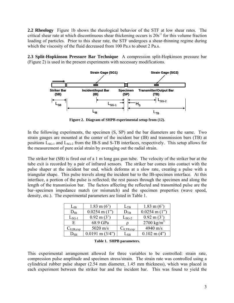
2.3 Split-Hopkinson Pressure Bar Technique A compression split-Hopkinson pressure bar (Figure 2) is used in the present experiments with necessary modifications.

Striker Bar(SB)

Incident/Input Bar(IB)

Transmitter/Output Bar(TB)

Specimen(SP)

Strain Gage (SG1) Strain Gage (SG2)

LIB LTB

LSG-1

LSG-2HSLSB

Striker Bar(SB)

Incident/Input Bar(IB)

Transmitter/Output Bar(TB)

Specimen(SP)

Strain Gage (SG1) Strain Gage (SG2)

LIB LTB

LSG-1

LSG-2HSLSB

Figure 2. Diagram of SHPB experimental setup from (12).

In the following experiments, the specimen (S, SP) and the bar diameters are the same. Two strain gauges are mounted at the center of the incident bar (IB) and transmission bars (TB) at positions LSG-1 and LSG-2 from the IB-S and S-TB interfaces, respectively. This setup allows for the measurement of pure axial strain by averaging out the radial strain. The striker bar (SB) is fired out of a 1 m long gas gun tube. The velocity of the striker bar at the tube exit is recorded by a pair of infrared sensors. The striker bar comes into contact with the pulse shaper at the incident bar end, which deforms at a slow rate, creating a pulse with a triangular shape. This pulse travels along the incident bar to the IB-specimen interface. At this interface, a portion of the pulse is reflected; the rest passes through the specimen and along the length of the transmission bar. The factors affecting the reflected and transmitted pulse are the bar–specimen impedance match (or mismatch) and the specimen properties (wave speed, density, etc.). The experimental parameters are listed in Table 1.

LIB 1.83 m (6’) LTB 1.83 m (6’) DIB 0.0254 m (1”) DTB 0.0254 m (1”)

LSG-1 0.92 m (3’) LSG-2 0.92 m (3’) E 68.9 GPa ρ 2700 kg/m3

C0,IB,exp 5020 m/s C0,TB,exp 4940 m/s DSB 0.0191 m (3/4”) LSB 0.102 m (4”)

Table 1. SHPB parameters.

This experimental arrangement allowed for three variables to be controlled: strain rate, compression pulse amplitude and specimen stress/strain. The strain rate was controlled using a cylindrical rubber pulse shaper (2.54 mm diameter, 1.45 mm thickness), which was placed in each experiment between the striker bar and the incident bar. This was found to yield the

4

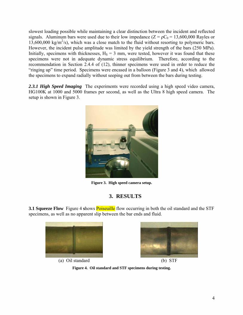
slowest loading possible while maintaining a clear distinction between the incident and reflected signals. Aluminum bars were used due to their low impedance (Z = ρC0 = 13,600,000 Rayles or 13,600,000 kg/m2/s), which was a close match to the fluid without resorting to polymeric bars. However, the incident pulse amplitude was limited by the yield strength of the bars (250 MPa). Initially, specimens with thicknesses, HS = 3 mm, were tested, however it was found that these specimens were not in adequate dynamic stress equilibrium. Therefore, according to the recommendation in Section 2.4.4 of (12), thinner specimens were used in order to reduce the “ringing up” time period. Specimens were encased in a balloon (Figure 3 and 4), which allowed the specimens to expand radially without seeping out from between the bars during testing. 2.3.1 High Speed Imaging The experiments were recorded using a high speed video camera, HG100K at 1000 and 5000 frames per second, as well as the Ultra 8 high speed camera. The setup is shown in Figure 3.

Figure 3. High speed camera setup.

3. RESULTS

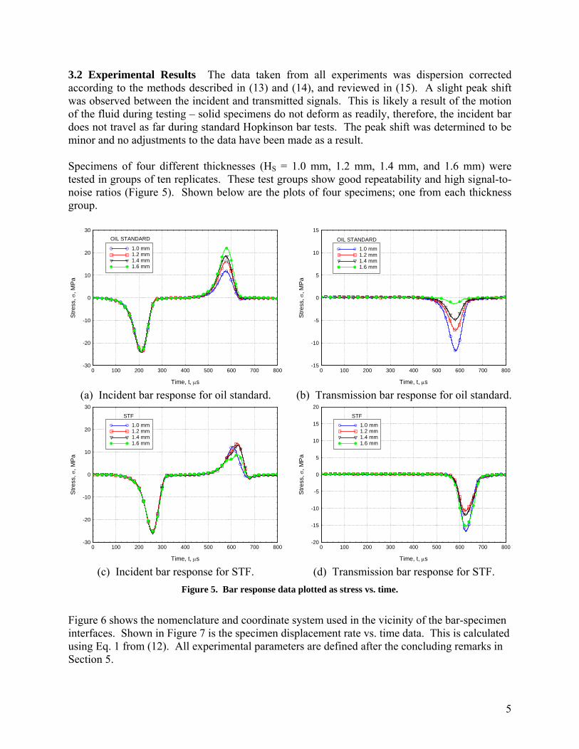
3.1 Squeeze Flow Figure 4 shows Poiseuille flow occurring in both the oil standard and the STF specimens, as well as no apparent slip between the bar ends and fluid.

(a) Oil standard (b) STF

Figure 4. Oil standard and STF specimens during testing.

5

3.2 Experimental Results The data taken from all experiments was dispersion corrected according to the methods described in (13) and (14), and reviewed in (15). A slight peak shift was observed between the incident and transmitted signals. This is likely a result of the motion of the fluid during testing – solid specimens do not deform as readily, therefore, the incident bar does not travel as far during standard Hopkinson bar tests. The peak shift was determined to be minor and no adjustments to the data have been made as a result. Specimens of four different thicknesses (HS = 1.0 mm, 1.2 mm, 1.4 mm, and 1.6 mm) were tested in groups of ten replicates. These test groups show good repeatability and high signal-to-noise ratios (Figure 5). Shown below are the plots of four specimens; one from each thickness group.

-30

-20

-10

0

10

20

30

0 100 200 300 400 500 600 700 800

1.0 mm1.2 mm1.4 mm1.6 mm

OIL STANDARD

Time, t, μs

Stre

ss, σ

, MPa

-15

-10

-5

0

5

10

15

0 100 200 300 400 500 600 700 800

1.0 mm1.2 mm1.4 mm1.6 mm

OIL STANDARD

Time, t, μs

Stre

ss, σ

, MPa

(a) Incident bar response for oil standard. (b) Transmission bar response for oil standard.

-30

-20

-10

0

10

20

30

0 100 200 300 400 500 600 700 800

1.0 mm1.2 mm1.4 mm1.6 mm

STF

Time, t, μs

Stre

ss, σ

, MPa

-20

-15

-10

-5

0

5

10

15

20

0 100 200 300 400 500 600 700 800

1.0 mm1.2 mm1.4 mm1.6 mm

STF

Time, t, μs

Stre

ss, σ

, MPa

(c) Incident bar response for STF. (d) Transmission bar response for STF. Figure 5. Bar response data plotted as stress vs. time.

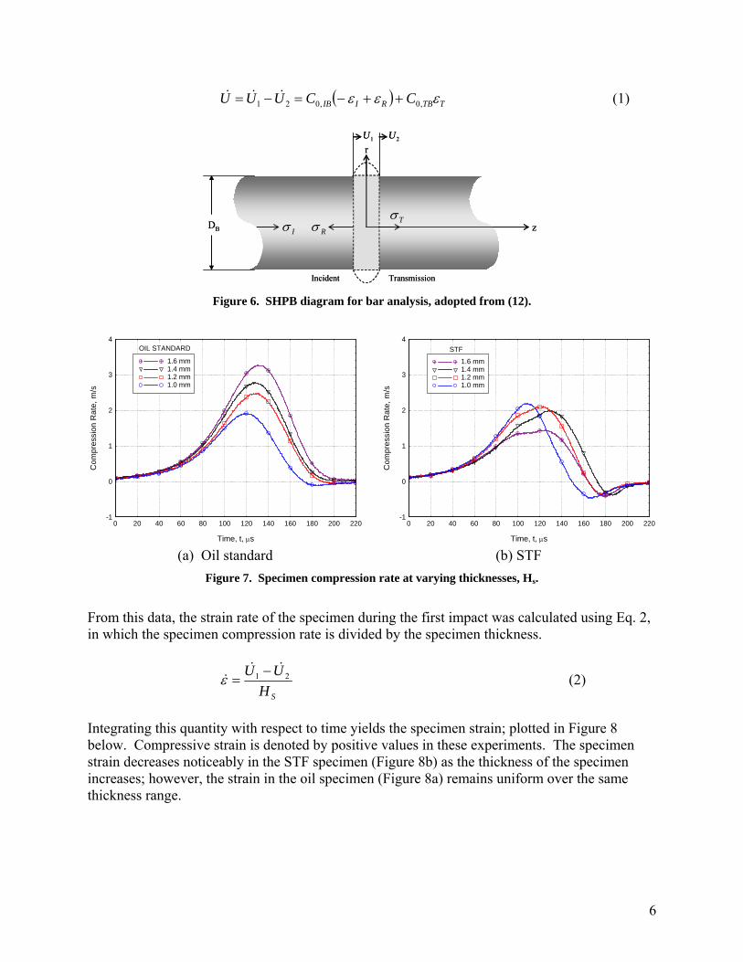
Figure 6 shows the nomenclature and coordinate system used in the vicinity of the bar-specimen interfaces. Shown in Figure 7 is the specimen displacement rate vs. time data. This is calculated using Eq. 1 from (12). All experimental parameters are defined after the concluding remarks in Section 5.

6

( ) TTBRIIB CCUUU εεε ,0,021 ++−=−= &&& (1)

F

r

z

1U 2U

TransmissionIncident

Iσ Rσ TσDB

F

r

z

1U 2U

TransmissionIncident

Iσ Rσ TσDB

Figure 6. SHPB diagram for bar analysis, adopted from (12).

-1

0

1

2

3

4

0 20 40 60 80 100 120 140 160 180 200 220

1.6 mm1.4 mm1.2 mm1.0 mm

OIL STANDARD

Time, t, μs

Com

pres

sion

Rat

e, m

/s

-1

0

1

2

3

4

0 20 40 60 80 100 120 140 160 180 200 220

1.6 mm1.4 mm1.2 mm1.0 mm

STF

Time, t, μs

Com

pres

sion

Rat

e, m

/s

(a) Oil standard (b) STF Figure 7. Specimen compression rate at varying thicknesses, Hs.

From this data, the strain rate of the specimen during the first impact was calculated using Eq. 2, in which the specimen compression rate is divided by the specimen thickness.

SHUU 21&&

&−

=ε (2)

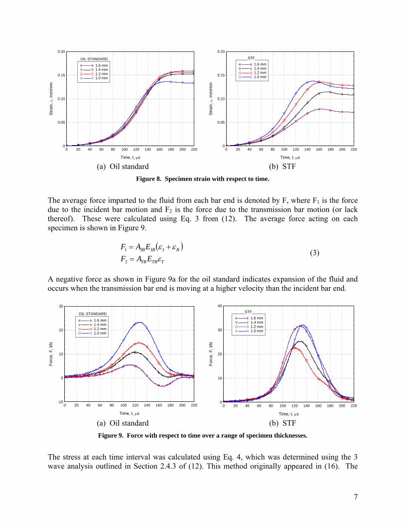
Integrating this quantity with respect to time yields the specimen strain; plotted in Figure 8 below. Compressive strain is denoted by positive values in these experiments. The specimen strain decreases noticeably in the STF specimen (Figure 8b) as the thickness of the specimen increases; however, the strain in the oil specimen (Figure 8a) remains uniform over the same thickness range.

7

0

0.05

0.10

0.15

0.20

0 20 40 60 80 100 120 140 160 180 200 220

1.6 mm1.4 mm1.2 mm1.0 mm

OIL STANDARD

Time, t, μs

Stra

in, ε

, mm

/mm

0

0.05

0.10

0.15

0.20

0 20 40 60 80 100 120 140 160 180 200 220

1.6 mm1.4 mm1.2 mm1.0 mm

STF

Time, t, μs

Stra

in, ε

, mm

/mm

(a) Oil standard (b) STF Figure 8. Specimen strain with respect to time.

The average force imparted to the fluid from each bar end is denoted by F, where F1 is the force due to the incident bar motion and F2 is the force due to the transmission bar motion (or lack thereof). These were calculated using Eq. 3 from (12). The average force acting on each specimen is shown in Figure 9.

( )TTBTB

RIIBIB

EAFEAF

εεε

=+=

2

1 (3)

A negative force as shown in Figure 9a for the oil standard indicates expansion of the fluid and occurs when the transmission bar end is moving at a higher velocity than the incident bar end.

-10

0

10

20

30

0 20 40 60 80 100 120 140 160 180 200 220

1.6 mm1.4 mm1.2 mm1.0 mm

OIL STANDARD

Time, t, μs

Forc

e, F

, kN

0

10

20

30

40

0 20 40 60 80 100 120 140 160 180 200 220

1.6 mm1.4 mm1.2 mm1.0 mm

STF

Time, t, μs

Forc

e, F

, kN

(a) Oil standard (b) STF Figure 9. Force with respect to time over a range of specimen thicknesses.

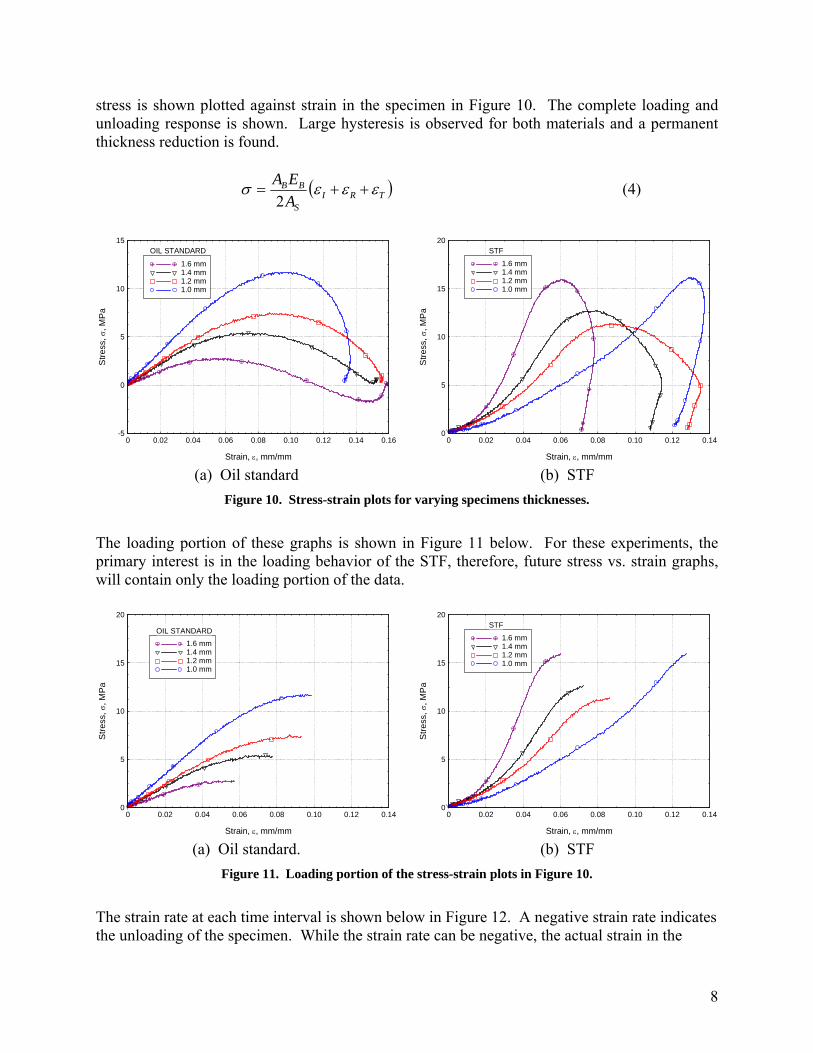
The stress at each time interval was calculated using Eq. 4, which was determined using the 3 wave analysis outlined in Section 2.4.3 of (12). This method originally appeared in (16). The

8

stress is shown plotted against strain in the specimen in Figure 10. The complete loading and unloading response is shown. Large hysteresis is observed for both materials and a permanent thickness reduction is found.

( )TRIS

BB

AEA εεεσ ++=

2 (4)

-5

0

5

10

15

0 0.02 0.04 0.06 0.08 0.10 0.12 0.14 0.16

1.6 mm1.4 mm1.2 mm1.0 mm

OIL STANDARD

Strain, ε, mm/mm

Stre

ss, σ

, MP

a

0

5

10

15

20

0 0.02 0.04 0.06 0.08 0.10 0.12 0.14

1.6 mm1.4 mm1.2 mm1.0 mm

STF

Strain, ε, mm/mm

Stre

ss, σ

, MP

a

(a) Oil standard (b) STF Figure 10. Stress-strain plots for varying specimens thicknesses.

The loading portion of these graphs is shown in Figure 11 below. For these experiments, the primary interest is in the loading behavior of the STF, therefore, future stress vs. strain graphs, will contain only the loading portion of the data.

0

5

10

15

20

0 0.02 0.04 0.06 0.08 0.10 0.12 0.14

1.6 mm1.4 mm1.2 mm1.0 mm

OIL STANDARD

Strain, ε, mm/mm

Stre

ss, σ

, MP

a

0

5

10

15

20

0 0.02 0.04 0.06 0.08 0.10 0.12 0.14

1.6 mm1.4 mm1.2 mm1.0 mm

STF

Strain, ε, mm/mm

Stre

ss, σ

, MP

a

(a) Oil standard. (b) STF Figure 11. Loading portion of the stress-strain plots in Figure 10.

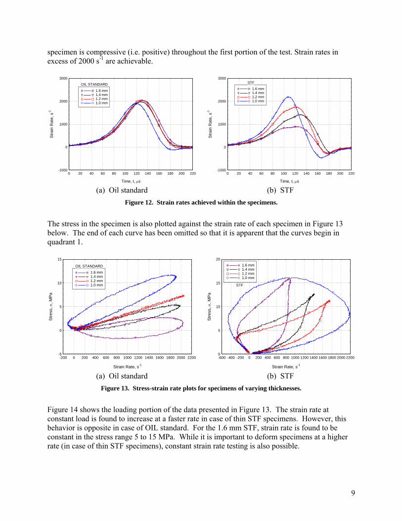
The strain rate at each time interval is shown below in Figure 12. A negative strain rate indicates the unloading of the specimen. While the strain rate can be negative, the actual strain in the

9

specimen is compressive (i.e. positive) throughout the first portion of the test. Strain rates in excess of 2000 s-1 are achievable.

-1000

0

1000

2000

3000

0 20 40 60 80 100 120 140 160 180 200 220

1.6 mm1.4 mm1.2 mm1.0 mm

OIL STANDARD

Time, t, μs

Stra

in R

ate,

s-1

-1000

0

1000

2000

3000

0 20 40 60 80 100 120 140 160 180 200 220

1.6 mm1.4 mm1.2 mm1.0 mm

STF

Time, t, μs

Stra

in R

ate,

s-1

(a) Oil standard (b) STF Figure 12. Strain rates achieved within the specimens.

The stress in the specimen is also plotted against the strain rate of each specimen in Figure 13 below. The end of each curve has been omitted so that it is apparent that the curves begin in quadrant 1.

-5

0

5

10

15

-200 0 200 400 600 800 1000 1200 1400 1600 1800 2000 2200

1.6 mm1.4 mm1.2 mm1.0 mm

OIL STANDARD

Strain Rate, s-1

Stre

ss, σ

, MP

a

0

5

10

15

20

-600 -400 -200 0 200 400 600 800 1000 1200 1400 1600 1800 2000 2200

1.6 mm1.4 mm1.2 mm1.0 mm

STF

Strain Rate, s-1

Stre

ss, σ

, MP

a

(a) Oil standard (b) STF Figure 13. Stress-strain rate plots for specimens of varying thicknesses.

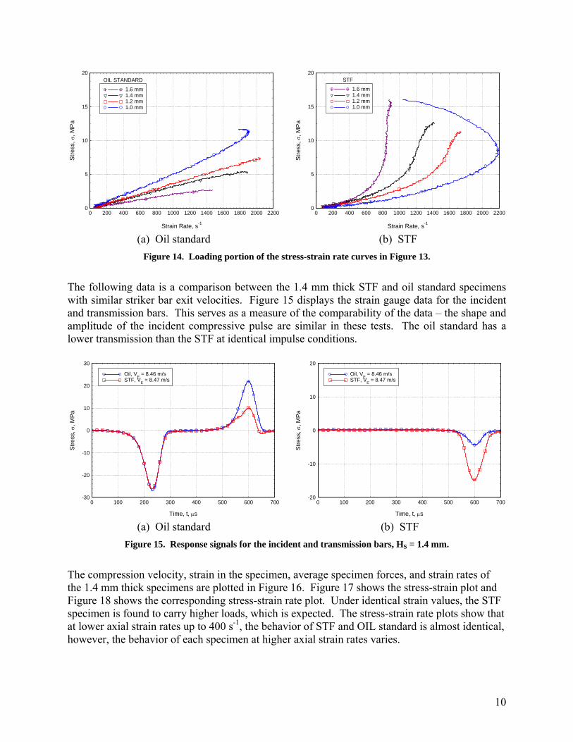
Figure 14 shows the loading portion of the data presented in Figure 13. The strain rate at constant load is found to increase at a faster rate in case of thin STF specimens. However, this behavior is opposite in case of OIL standard. For the 1.6 mm STF, strain rate is found to be constant in the stress range 5 to 15 MPa. While it is important to deform specimens at a higher rate (in case of thin STF specimens), constant strain rate testing is also possible.

10

0

5

10

15

20

0 200 400 600 800 1000 1200 1400 1600 1800 2000 2200

1.6 mm1.4 mm1.2 mm1.0 mm

OIL STANDARD

Strain Rate, s-1

Stre

ss, σ

, MP

a

0

5

10

15

20

0 200 400 600 800 1000 1200 1400 1600 1800 2000 2200

1.6 mm1.4 mm1.2 mm1.0 mm

STF

Strain Rate, s-1

Stre

ss, σ

, MP

a

(a) Oil standard (b) STF Figure 14. Loading portion of the stress-strain rate curves in Figure 13.

The following data is a comparison between the 1.4 mm thick STF and oil standard specimens with similar striker bar exit velocities. Figure 15 displays the strain gauge data for the incident and transmission bars. This serves as a measure of the comparability of the data – the shape and amplitude of the incident compressive pulse are similar in these tests. The oil standard has a lower transmission than the STF at identical impulse conditions.

-30

-20

-10

0

10

20

30

0 100 200 300 400 500 600 700

Oil, VE = 8.46 m/sSTF, VE = 8.47 m/s

Time, t, μs

Stre

ss, σ

, MPa

-20

-10

0

10

20

0 100 200 300 400 500 600 700

Oil, VE = 8.46 m/sSTF, VE = 8.47 m/s

Time, t, μs

Stre

ss, σ

, MPa

(a) Oil standard (b) STF Figure 15. Response signals for the incident and transmission bars, HS = 1.4 mm.

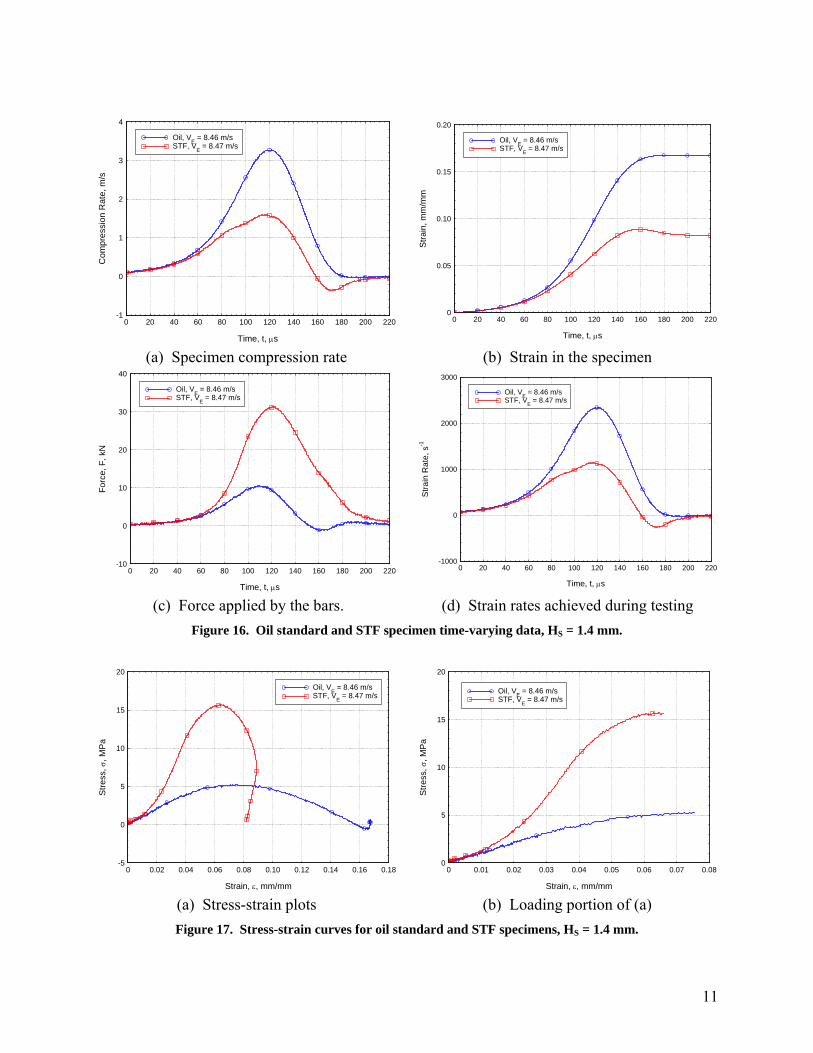
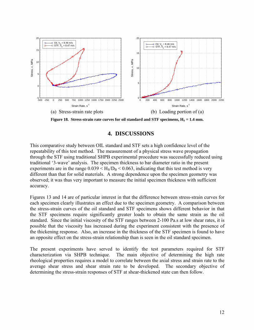
The compression velocity, strain in the specimen, average specimen forces, and strain rates of the 1.4 mm thick specimens are plotted in Figure 16. Figure 17 shows the stress-strain plot and Figure 18 shows the corresponding stress-strain rate plot. Under identical strain values, the STF specimen is found to carry higher loads, which is expected. The stress-strain rate plots show that at lower axial strain rates up to 400 s-1, the behavior of STF and OIL standard is almost identical, however, the behavior of each specimen at higher axial strain rates varies.

11

-1

0

1

2

3

4

0 20 40 60 80 100 120 140 160 180 200 220

Oil, VE = 8.46 m/sSTF, VE = 8.47 m/s

Time, t, μs

Com

pres

sion

Rat

e, m

/s

0

0.05

0.10

0.15

0.20

0 20 40 60 80 100 120 140 160 180 200 220

Oil, VE = 8.46 m/sSTF, VE = 8.47 m/s

Time, t, μs

Stra

in, m

m/m

m

(a) Specimen compression rate (b) Strain in the specimen

-10

0

10

20

30

40

0 20 40 60 80 100 120 140 160 180 200 220

Oil, VE = 8.46 m/sSTF, VE = 8.47 m/s

Time, t, μs

Forc

e, F

, kN

-1000

0

1000

2000

3000

0 20 40 60 80 100 120 140 160 180 200 220

Oil, VE = 8.46 m/sSTF, VE = 8.47 m/s

Time, t, μs

Stra

in R

ate,

s-1

(c) Force applied by the bars. (d) Strain rates achieved during testing Figure 16. Oil standard and STF specimen time-varying data, HS = 1.4 mm.

-5

0

5

10

15

20

0 0.02 0.04 0.06 0.08 0.10 0.12 0.14 0.16 0.18

Oil, VE = 8.46 m/sSTF, VE = 8.47 m/s

Strain, ε, mm/mm

Stre

ss, σ

, MPa

0

5

10

15

20

0 0.01 0.02 0.03 0.04 0.05 0.06 0.07 0.08

Oil, VE = 8.46 m/sSTF, VE = 8.47 m/s

Strain, ε, mm/mm

Stre

ss, σ

, MPa

(a) Stress-strain plots (b) Loading portion of (a) Figure 17. Stress-strain curves for oil standard and STF specimens, HS = 1.4 mm.

12

-5

0

5

10

15

20

-500 -250 0 250 500 750 1000 1250 1500 1750 2000 2250 2500

Oil, VE = 8.46 m/sSTF, VE = 8.47 m/s

Strain Rate, s-1

Stre

ss, σ

, MPa

0

5

10

15

20

0 200 400 600 800 1000 1200 1400 1600 1800 2000 2200

Oil, VE = 8.46 m/sSTF, VE = 8.47 m/s

Strain Rate, s-1

Stre

ss, σ

, MPa

(a) Stress-strain rate plots (b) Loading portion of (a) Figure 18. Stress-strain rate curves for oil standard and STF specimens, HS = 1.4 mm.

4. DISCUSSIONS

This comparative study between OIL standard and STF sets a high confidence level of the repeatability of this test method. The measurement of a physical stress wave propagation through the STF using traditional SHPB experimental procedure was successfully reduced using traditional ‘3-wave’ analysis. The specimen thickness to bar diameter ratio in the present experiments are in the range 0.039 < HS/DB < 0.063, indicating that this test method is very different than that for solid materials. A strong dependence upon the specimen geometry was observed; it was thus very important to measure the initial specimen thickness with sufficient accuracy. Figures 13 and 14 are of particular interest in that the difference between stress-strain curves for each specimen clearly illustrates an effect due to the specimen geometry. A comparison between the stress-strain curves of the oil standard and STF specimens shows different behavior in that the STF specimens require significantly greater loads to obtain the same strain as the oil standard. Since the initial viscosity of the STF ranges between 2-100 Pa.s at low shear rates, it is possible that the viscosity has increased during the experiment consistent with the presence of the thickening response. Also, an increase in the thickness of the STF specimen is found to have an opposite effect on the stress-strain relationship than is seen in the oil standard specimen. The present experiments have served to identify the test parameters required for STF characterization via SHPB technique. The main objective of determining the high rate rheological properties requires a model to correlate between the axial stress and strain rate to the average shear stress and shear strain rate to be developed. The secondary objective of determining the stress-strain responses of STF at shear-thickened state can then follow.

13

5. CONCLUSIONS

A novel test method for the dynamic squeeze flow of a fluid has been developed and found to yield uniform repeatable results. This modified split Hopkinson pressure bar technique can achieve over 2000 s-1 in thin fluid specimens while remaining in a stress range an order of magnitude lower than the bar yield strength. It should be noted that these strain rates are an order of magnitude higher than that produced by typical rheometers. In addition, this technique can also achieve high compressive stress levels to characterize the STF in the post-transition state. Possible evidence of shear thickening was also observed through the comparison of the stress vs. strain plots of the oil standard and STF fluid. Future work will include more advanced data reduction using a recently developed model to extract the viscosity data due to the applied strain rate, to quantify geometric factors and isolate STF constitutive response. Nomenclature

Iε incident strain

Rε reflected strain

Tε transmitted strain ε& strain rate σ stress

1U& particle velocity at incident bar end

2U& particle velocity at transmission bar end

1U incident bar end displacement

2U transmission bar end displacement

EV striker bar exit velocity

IBL incident bar length

TBL transmission bar length

IBD incident bar diameter

TBD transmission bar diameter

1−SGL distance between IB-specimen interface and IB strain gage

2−GSL distance between TB-specimen interface and TB strain gage E Young’s modulus

SBL striker bar length

SBD striker bar diameter

SH initial specimen thickness

0C wave speed ρ density η viscosity

BA bar cross-sectional area

SBA striker bar cross-sectional area

14

SA specimen cross-sectional area F force acting upon the fluid Acknowledgements This project is funded through the Army Research Office. The authors would like to acknowledge Dr. Norman J. Wagner, Dr. Eric D. Wetzel, and Dr. Joseph M. Deitzel for their helpful discussions, as well as Dr. Caroline Nam for providing the shear-thickening fluid used in these experiments, as well as the rheology data in Figure 1b. Dr. Sergey L. Lopatnikov has also been instrumental in the modeling of this experiment.

6. REFERENCES 1. Lee, Y.S. and N.J. Wagner, Dynamic properties of shear thickening colloidal

suspensions. Rheo Acta., 42, 199-208 (2003). 2. Lee, Y.S., et al. Advanced body armor utilizing shear thickening fluids. 23rd Army

Science Conference. Orlando, FL (2002). 3. Lee, Y.S., E.D. Wetzel, and N.J. Wagner. The ballistic impact characteristics of Kevlar

woven fabrics impregnated with a colloidal shear thickening fluid. Journal of Materials Science, 38, 2825-2833 (2003).

4. Wetzel, E.D., et al. The effect of rheological parameters on the ballistic properties of shear thickening fluid (STF)-Kevlar composites. Materials Processing and Design: Modeling, Simulation and Applications, 288-293 (2004).

5. R. G. Egres, J., et al. Protective fabrics utilizing shear thickening fluids. Industrial Fabrics Association International 4th International Conference on Safety and Protective Fabrics. Pittsburgh, PA (2004)

6. R. G. Egres, J., et al. Stab resistance of shear thickening fluid (STF)-Kevlar composites for body armor applications. 24th Army Science Conference. Orlando, FL (2004).

7. R. G. Egres, J., et al. Stab performance of shear thickening fluid (STF) - fabric composites for body armor applications. SAMPE 2005: New Horizons for Materials and Processing Technologies. Long Beach, CA. (2005).

8. Decker, M.J., et al. Low velocity ballistic properties of shear thickening fluid (STF)-fabric composites. 22nd International Symposium on Ballistics. 2005.

9. Nam, C.H., et al. Ballistic and rheological properties of STFs reinforced by short discontinuous fibers. SAMPE 2005: New Horizons for Materials and Processing Technologies. Long Beach, CA (2005).

10. Bender, J. and Wagner, N. J. Reversible shear thickening in monodisperse and bidisperse colloidal dispersions. J. Rheol. 40 (5), 899-916 (1996).

11. Maranzano, B. J. and Wagner, N.J. Shear thickening rheology of near hard-sphere colloidal suspensions. Proceedings of the XIIIth International Congress on Rheology., 261-263 (2000).

12. Gama, B. A. Split Hopkinson Pressure Bar Technique: Experiments, Analyses and Applications. University of Delaware, 2004, pp. 80-85.

13. Lifshitz, J. M. and Leber, H. Data processing in the split Hopkinson pressure bar tests. Int. J. Impact Eng., 15 (6), 723-733 (1994).

14. Li Z. and Lambros J. Determination of the dynamic response of brittle composites by the use of split Hopkinson pressure bar. Compos. Sci. Tech., 59, 1097-1107 (1999).

15

15. Gama, B. A., Lopatnikov, S. L, and Gillespie Jr., J. W. Hopkinson Bar Experimental Technique: A Critical Review. Applied Mechanics Review., 57, (4) (2004).

16. Grey III, G. T. Classic Split-Hopkinson Pressure Bar Testing. ASM Handbook – 8, Mechanical Testing and Evaluation, ASM International, Materials Park, Ohio, 488-496 (2000).