High School Track Choice and Financial Constraints

Policy Research Working Paper 7427

High School Track Choice and Financial Constraints

Evidence from Urban Mexico

Ciro AvitabileMatteo Bobba

Marco Pariguana

Education Global Practice GroupSeptember 2015

WPS7427P

ublic

Dis

clos

ure

Aut

horiz

edP

ublic

Dis

clos

ure

Aut

horiz

edP

ublic

Dis

clos

ure

Aut

horiz

edP

ublic

Dis

clos

ure

Aut

horiz

ed

Produced by the Research Support Team

Abstract

The Policy Research Working Paper Series disseminates the findings of work in progress to encourage the exchange of ideas about development issues. An objective of the series is to get the findings out quickly, even if the presentations are less than fully polished. The papers carry the names of the authors and should be cited accordingly. The findings, interpretations, and conclusions expressed in this paper are entirely those of the authors. They do not necessarily represent the views of the International Bank for Reconstruction and Development/World Bank and its affiliated organizations, or those of the Executive Directors of the World Bank or the governments they represent.

Policy Research Working Paper 7427

This paper is a product of the Education Global Practice Group. It is part of a larger effort by the World Bank to provide open access to its research and make a contribution to development policy discussions around the world. Policy Research Working Papers are also posted on the Web at http://econ.worldbank.org. The authors may be contacted at [email protected].

Parents and students from different socioeconomic back-grounds value differently school characteristics, but the reasons behind this preference heterogeneity are not well understood. In the context of the centralized school assignment system in Mexico City, this study analyzes how a large household income shock affects choices over high school tracks exploiting the discontinuity in

the assignment of the welfare program Oportunidades. The income shock significantly increases the probabil-ity of choosing the vocational track vis-a-vis the other more academic-oriented tracks. The findings suggest that the transfer relaxes the financial constraints that prevent relatively low-ability students from choosing the schooling option with higher labor market returns.

High School Track Choice and Financial Constraints:

Evidence From Urban Mexico

Ciro Avitabile∗ Matteo Bobba† Marco Pariguana‡

∗The World Bank. E-mail: [email protected].†Toulouse School of Economics. E-mail: [email protected].‡Pennsylvania State University. E-mail: [email protected].

1 Introduction

Differences in socioeconomic status are associated with significant variation in the weights that

parents and students place on important school characteristics - e.g. quality of peers, distance,

ethnic composition [Hastings et al., 2008; Burgess et al., 2009]. Nevertheless it is unclear to

what extent these disparate valuations are the result of financial constraints or reflect differences in

unobserved characteristics, such as the level of information, social norms and idiosyncratic tastes.1

This paper studies how a large household income shock can affect stated preferences over high

school tracks of relatively disadvantaged youths living in a suburban district of Mexico City.2

School track choice can have important consequences on future academic trajectories and la-

bor market outcomes [Dustmann et al., 2014; Kerr et al., 2013]. Countries differ widely on the

degree to which they track students, and the age at which students begin to be tracked.3 Within-

school ability grouping is common in the United States and Canada, while curricular tracking at

the secondary level is widespread in many countries (see continental Europe and Latin America).

Mexico is a particularly interesting context to study high school track choices. When completing

middle school, students can choose among three different education modalities (general, technical

and vocational), that greatly differ in the extent to which they prepare students to enter the labor

market. Only 9% of high school students enroll in the vocational track - this is extremely low

not only compared to the OECD average (44%), but also to other countries in Latin America (see

Table 1). Only six out of ten students who enroll in upper secondary education successfully gradu-

ate, and graduation rates vary across high school tracks with general schools featuring the highest

(64%), followed by technical schools (61%) and vocational schools (48%) (Ministry of Education

2013). Against this backdrop, it is unclear the extent to which the large dropout rate is related to

the mismatch between students and the high school curriculum.

The centralized assignment mechanism in the metropolitan area of Mexico City, which allo-

1Evidence from a variety of settings suggests that school choices are systematically correlated with socioeconomicbackground, even after controlling for pre-determined measures of ability (e.g. test scores) - see, for instance, Ajayi[2013] for evidence on Ghana and Avery and Hoxby [2012] for the US case.

2Throughout the paper we will use upper secondary education and high school indifferently when we refer togrades 10 to 12. We will use middle school and junior high school indifferently when referring to grades 7 to 9.

3Definitions of tracking in the academic literature range from nothing more than ability grouping to more elaborateforms that divide students by academic achievement with the explicit intent of delivering a different curriculum, andusing different pedagogical methods, for different groups of students (see, e.g., Betts [2011] for a review).

2

cates students to public high schools, offers an ideal setting to study school preferences and their

determinants. The matching algorithm is strategy-proof, which gives us the unique opportunity to

infer preferences from individual choices over the quasi-universe of public high school programs in

the area. In this context, we explore how financial constraints can affect high school track choices

using the assignment of the welfare program Oportunidades as a positive shock to household in-

come. The size of the transfer is sizable, amounting to roughly one-third of the median household

income in our sample, and the discontinuity in the program assignment based on a pre-determined

poverty score allows us to tease out the causal effects of the transfer by comparing households just

above and just below the eligibility threshold.

Our estimates show that eligibility for the Oportunidades cash transfers increases the probabil-

ity of choosing the vocational track as first high school option by 4 percentage points. When we

account for the imperfect compliance with the program, we find that the probability of choosing

the vocational track as first option increases by 6.1 percentage point, which is equivalent to a nearly

55% increase with respect to the sample average. This result is robust across different estimators

and specifications. We rule out that the observed changes in students’ preferences across tracks are

partly driven by program-induced changes in the composition of high school applicants.

Additional evidence gathered from a variety of auxiliary data sources allows us characterizing

the costs and benefits of attending different tracks in the context of the COMIPEMS system. When

compared to the other more academic-oriented tracks, the vocational track seems indeed to entail

a higher financial burden for the poor households in our sample - in terms of both tuition and

transportation costs. At the same time, the vocational track is associated with higher labor market

returns for those individuals who enter the labor market after completing high school, perhaps due

to the presence of a tighter link between the type of contents offered by those programs and the

characteristics of the local labor markets under study. Accordingly, we find that the effect of the

cash transfer on the probability of choosing a vocational option is concentrated among lower ability

applicants (in terms of their academic achievement in junior high school), and for those with more

difficult access to vocational programs (in terms of higher distance from their places of residence).

Irrespectively of the educational track, cash transfers seem to shift students’ preferred choices

toward schools that are located further away from their places of residence and with higher tuition

fees. When investigating the potential behavioral responses associated with the change in school

3

preferences, we find no support either for the hypothesis that a) students’ strategically alter their

school choice portfolio in order to increase the expected value of the future stream of cash transfers,

or that b) students opt for more selective schools. Based on this evidence, we argue that cash

transfers affect school preferences in our setting by relaxing the financial constraints that prevent

students from choosing the high school track with the highest expected returns.

Changes in track choices induced by the receipt of the cash transfers may also have persistent

impacts on educational trajectories later on. In order to inspect this possibility, we exploit another

key feature of the COMIPEMS mechanism: placement in the system solely depends on students’

elicited preferences and their performance in the admission exam. Since we can measure any

change in those two outcomes induced by the receipt of the cash transfers, we are also able to

track the effects on high school assignment and longer-term educational outcomes. We find some

suggestive evidence that, for students with tighter liquidity constraints, the observed changes in

students’ preferences over schools translate into a higher probability of being assigned to their

most preferred schooling option, as well as into a lower drop-out rate during high school.

This paper broadly speaks to a large body of literature that explores the effects of credit market

frictions on human capital investments (see, e.g., Lochner and Monge-Naranjo [2012] for a recent

review). Most of the existing literature on school choice decisions considers the role of infor-

mation frictions. Increasing evidence shows that the degree of accuracy of information about the

characteristics of the available schooling alternatives [Ajayi, 2013; Avery and Hoxby, 2012; Bet-

tinger et al., 2012; Dinkelman and Martinez, 2014; Hastings and Weinstein, 2008; Lai et al., 2009;

Mizala and Urquiola, 2013] and their associated labor market earnings [Arcidiacono, 2004, 2005;

Attanasio and Kaufmann, forthcoming; Kaufmann, forthcoming; Jensen, 2010; Wiswall and Zafar,

forthcoming] play a role for both students’ and parents’ decision making. Our paper contributes

to this strand of literature by pointing to the potential role of financial frictions underlying school

choice decisions. Overall, our results can be interpreted as evidence that in a developing country

context financial constraints can be partly responsible for the mismatch between school type and

student ability. We contribute to the literature that studies school preferences [Deming et al., 2014;

Hastings et al., 2008; Burgess et al., 2009], showing that at high school level the academic track is

an important variable that students weight when making their choices.

Most closely related to our paper, Giustinelli [2014] studies how subjective expected utilities of

4

both parents and students shape high school track choices. In the same context under study in this

paper, Bobba and Frisancho [2014] focus on the role of students’ self-perceptions about academic

ability as a potential source of distortion for perceived track-specific returns and hence high school

choice decisions, while De Janvry et al. [2013] highlights the potential trade-off between drop-out

risk and academic benefit behind students’ demand for “elite” public high schools.

2 Context and Data

2.1 The School Assignment Mechanism

The Mexican system offers three educational modalities (tracks thereafter) at the higher secondary

level: General, Technical, and Vocational Education (Bachillerato General, Bachillerato Tec-

nológico, and Educación Profesional Técnica, respectively). The technical modalities include the

curriculum covered in a general education program but they also incorporate additional courses

that allow students to become a technician upon completion of higher secondary schooling. In

turn, a student who chose to get a vocational education is exclusively trained to become a pro-

fessional technician. From 2008 onwards, as result of the Integral Reform of Upper-Secondary

Education (RIEMS), all three modalities allow students to attend tertiary education, although the

timing of adaptation to the new system varied dramatically across states. As result, in the time

period covered by our analysis, the option value of attending tertiary education is the same for all

three modalities.

Students who want to attend a public high school in the urban area of Mexico City are required

to enroll in a centralized and competitive assignment mechanism regulated and administered by

the Metropolitan Commission of Higher Secondary Public Education Institutions (COMIPEMS,

by its Spanish acronym). Since 1996, the commission brings together nine institutions who have

agreed to select candidates through a standardized achievement exam.4 In 2007, these institutions

offered over 238,000 seats in about 700 public schools located in Mexico’s capital city as well as

4The nine institutions who offer schools through the COMIPEMS are: Universidad Nacional Autónoma de Méx-ico (UNAM), Instituto Politécnico Nacional (IPN), Universidad Autónoma del Estado de México (UAEM), ColegioNacional de Educación Profesional Técnica (CONALEP), Colegio de Bachilleres (COLBACH), Dirección General deEducación Tecnológica Industrial (DGETI), Dirección General de Educación Tecnológica Agropecuaria (DGETA),Secretaría de Educación del Gobierno del Estado de México (SE), and Dirección General del Bachillerato (DGB).

5

22 urban municipalities that surround the city.

More details about the COMIPEMS assignment mechanism can be found in Bobba and Fri-

sancho [2014] and Dustan [2014]. Here we stress some aspects of the context that make students’

rankings particularly informative about their underlying preferences over schooling alternatives.

First, administrative records capture individual revealed preference rankings over a wide range of

available high school alternatives, which allows us to accurately measure student-specific ranked

orderings over high school tracks. Second, the matching mechanism in place and the large portfolio

size that can be submitted imply that the assignment mechanism is strategy-proof [Pathak, 2011].

Since admission probabilities to each school do not play a role when choosing an application port-

folio, any effect on choices due to the receipt of the cash transfers is enabled through changes in

net expected benefits across high school tracks.5 Third, official information about school-level aca-

demic quality is publicly available. Past cutoff scores for each schooling option have been made

available through the COMIPEMS website since 2005.6 Since the cutoff scores and the mean score

of admitted students are almost perfectly correlated, students have access to an excellent proxy for

the average peer ability in each school.

2.2 The Oportunidades Program

Oportunidades is a conditional cash transfer program that targets poor households in both rural

and urban areas of Mexico.7 The program was first initiated in 1997 in rural areas of Mexico, and

by 2001 it began to expand at a rapid rate into semi-urban and urban areas reaching the urban area

under study in the second half of 2004. Cash transfers are given on a bimonthly basis to one of

adult household members (usually the mother) and come in two forms. The first is a fixed food

stipend which is worth 175 MX$ (around 16 US$) per month as of the first half of 2005 and it is

conditional on family members obtaining preventive medical care. The second is an educational

grant which is offered to each child aged 6-21 in the household. To receive the school subsidy,

children or youths in participating households have to attend school in one of the subsidy-eligible

5Even though students are allowed to rank up to twenty options only a minor percentage of them fills up the entirepreference sheet; students seem to be choosing a portfolio without binding constraints on the number of options thatcan be chosen.

6This site is frequently checked by the applicants because it has become the main channel to pre-register and it isalso a key source of information about the system.

7Details of the program can be found in Hoddinott and Skoufias [2004].

6

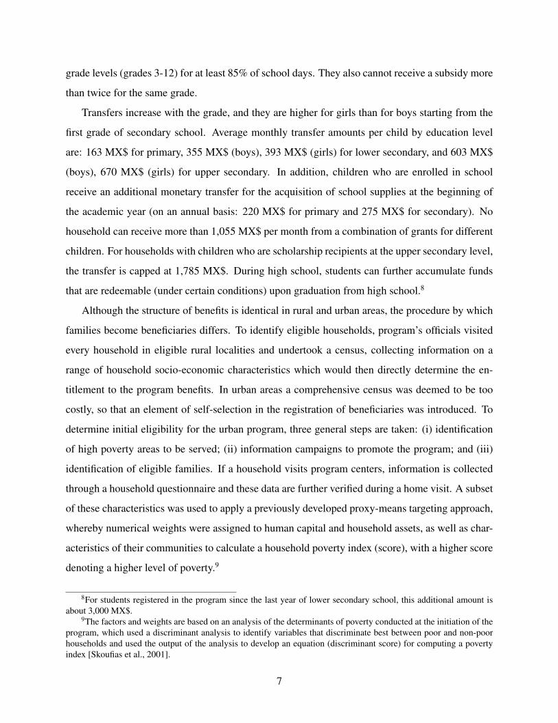
grade levels (grades 3-12) for at least 85% of school days. They also cannot receive a subsidy more

than twice for the same grade.

Transfers increase with the grade, and they are higher for girls than for boys starting from the

first grade of secondary school. Average monthly transfer amounts per child by education level

are: 163 MX$ for primary, 355 MX$ (boys), 393 MX$ (girls) for lower secondary, and 603 MX$

(boys), 670 MX$ (girls) for upper secondary. In addition, children who are enrolled in school

receive an additional monetary transfer for the acquisition of school supplies at the beginning of

the academic year (on an annual basis: 220 MX$ for primary and 275 MX$ for secondary). No

household can receive more than 1,055 MX$ per month from a combination of grants for different

children. For households with children who are scholarship recipients at the upper secondary level,

the transfer is capped at 1,785 MX$. During high school, students can further accumulate funds

that are redeemable (under certain conditions) upon graduation from high school.8

Although the structure of benefits is identical in rural and urban areas, the procedure by which

families become beneficiaries differs. To identify eligible households, program’s officials visited

every household in eligible rural localities and undertook a census, collecting information on a

range of household socio-economic characteristics which would then directly determine the en-

titlement to the program benefits. In urban areas a comprehensive census was deemed to be too

costly, so that an element of self-selection in the registration of beneficiaries was introduced. To

determine initial eligibility for the urban program, three general steps are taken: (i) identification

of high poverty areas to be served; (ii) information campaigns to promote the program; and (iii)

identification of eligible families. If a household visits program centers, information is collected

through a household questionnaire and these data are further verified during a home visit. A subset

of these characteristics was used to apply a previously developed proxy-means targeting approach,

whereby numerical weights were assigned to human capital and household assets, as well as char-

acteristics of their communities to calculate a household poverty index (score), with a higher score

denoting a higher level of poverty.9

8For students registered in the program since the last year of lower secondary school, this additional amount isabout 3,000 MX$.

9The factors and weights are based on an analysis of the determinants of poverty conducted at the initiation of theprogram, which used a discriminant analysis to identify variables that discriminate best between poor and non-poorhouseholds and used the output of the analysis to develop an equation (discriminant score) for computing a povertyindex [Skoufias et al., 2001].

7

2.3 Sample Description

Our analysis is restricted to households living in the town of Ecatepec de Morelos, which is lo-

cated in the Estado de Mexico in the outskirts of Mexico City’s Federal District.10 In 2004, a

census household survey (ENCASEH) was administered to 18,593 households to assess their el-

igibility for the Oportunidades transfer. The roster of the Oportunidades recipients for Ecatepec

de Morelos further allows to assess whether and when the households eligible for Oportunidades

started receiving any monetary grant.

For all the years between 2005 and 2010 we have information on the universe of COMIPEMS

applicants within the entire metropolitan area of Mexico City.11 The official data collected within

the COMIPEMS system feature students’ address of residence, socio-demographic characteristics

(gender, age, household income, parental education and occupation, personality traits, among oth-

ers) and schooling trajectories (GPA in lower secondary school, study habits, among others) as

well as the full ranked list of schooling options requested during the application process and re-

lated information about students’ placement in the system (including their score in the admission

exam).

All COMIPEMS applicants have a 16 digits unique student identifier (CURP), that is generated

by combining information on student’s name, surname, date of birth and state of birth, plus a

2 digit random generated number. All the relevant demographic information is collected by the

ENCASEH, allowing us to construct a “pseudo-CURP”, that only differs from the student identifier

in the 2 digit random generated number. After removing all the individuals for which we have

missing information or a “pseudo-CURP” that can be potentially matched with 2 or more CURPS,

we are left with a sample of 6,173 COMIPEMS applicants in the age group 14-20, for which we

have information on the proxy-means score used to assign the Oportunidades transfer.

After excluding those applicants that lack basic sociodemographic information, we are left with

a final sample of 5,232 students who applied in the COMIPEMS system during the period com-

10The Ecatepec municipality is the most densely populated in the country, with a population of 1,656,107 inhab-itants (INEGI 2010). In 2011, Ecatepec was third in the country’s poverty ranking , with 723,559 individuals livingunder the poverty line (CONEVAL). Ecatepec’s economy is based on industry, commerce and services. Over 1,550medium and small enterprises are registered in its territory. A large portion of the city’s inhabitants commute to theFederal District for labor or academic activities every day. The city also receives a large number of workers commutingfrom other municipalities.

11In this way we are able to track households that move outside the town of Ecatepec, but stay within the MexicoCity area.

8

prised between 2005 and 2010.12 Of those, 3,180 (61%) belong to households which were deemed

eligible for the Oportunidades benefits - i.e. the value of their proxy-mean score is greater or equal

than 0.69. Among eligible students, 2,161 (68%) are reported receiving at least one payment from

Oportunidades before applying to the COMIPEMS system.13 As a result of a process of program

expansion in urban areas which took place in the end of 2008, a very small fraction (1.2%) of

ineligible applicants in our sample are reported receiving some program benefits before applying

to the COMIPEMS system.

For the median household in our sample, the Oportunidades transfer is between 27 and 28

percent of total household income. The large size of the income shock in our sample likely reflects

the selection induced by the participation into the COMIPEMS system. When compared to the

rest of the families in the ENCASEH survey, those with at least one child who applies for upper

secondary education have in fact more children currently enrolled in grades 3-12. In fact, transfer

amount for program eligible families who are not in the COMIPEMS sample are substantially

lower: between 14 and 16 percent of total household income for the median household in our

sample.14

Only 9 percent of the COMIPEMS applicants in our sample list a vocational program as their

first option, while 44 percent and 47 percent of the applicants respectively opt for the technical

and the academic track. On average, when compared to the latter group of students, those who

prefer a vocational education tend to perform worse in school (as measured by the score in the

admission exam and in the cumulative grade point average in lower secondary), and they tend to

come from more disadvantaged socio-economic backgrounds (as measured by parental education,

the Oportunidades eligibility score and the relative share of those who report to be working - with

or without a wage).

12Only a small percentage (about 3%) of students who have filled the ranking of their preferred options, do nottake part in the COMIPEMS exam. We could not geocode the address of residence for roughly 10% of applicants.However, neither sample attrition rates vary systematically around the program eligibility threshold.

13Program take-up rates are fairly high when compared with the corresponding figures reported in the existingevaluation studies of the urban component of Oportunidades [Angelucci and Attanasio, 2009]. Previous studies usedthe urban evaluation surveys (ENCELURB) which entails roughly 18-24 months between program inception andobserved outcomes, whereas we observe eligible households for up to six years after program inception. In fact,take-up rates in our sample increase from 40% in 2005 to 79% in 2010.

14Those figures are in line with previous studies that considered the urban component of the Oportunidades pro-gram [Angelucci and Attanasio, 2013].

9

2.4 Auxiliary Data Sources

We combine the main sample described in the previous section with four administrative data

sources. First, the biannual Mexican school census which collects information on school-level

yearly trajectories - e.g. enrollment, failure and drop-out rate, school infrastructure, teachers’ and

school principals’ main characteristics as well as detailed information on the attendance fees that

students have to incur upon registration in a given school: tools, uniforms, monthly payments, reg-

istration and tuition. This information can be conveniently linked with the full list of COMIPEMS

schooling options through a unique school identifier (Claves de Centros de Trabajo - CCT) during

the period 2005-2010. In addition, geocoded information allows us to compute geodesic distances

between students’ places of residence and the high school programs offered by the COMIPEMS

system.

Second, we employ a sub-module of the third round of the 2008 national employment survey

(ENOE) which records retrospective information on the academic trajectories of individuals in the

age group 15-34, who passed at least one year of upper secondary education, including the track

attended in high school and whether college education was attended or not. Wage and employment

information comes from the ENOE that is considered the most reliable source of wage data for

Mexico. This survey is representative at the State-level and further allows to distinguish between

rural, semi-urban and urban areas depending on the population size of the communities of residence

of the surveyed individuals. We thus consider as the relevant labor market for the COMIPEMS

applicants in the city of Ecatepec the urban sections of the State of Mexico and the Federal District.

Third, we use data from a 2009 survey collected on a nationally-representative sample of stu-

dents who take a nationally standardized end of high school test (ENLACE). The so called EN-

LACE de contexto gathers, among others, information on expected monthly earnings five years

from the moment of the survey depending on two hypothetical scenarios of educational attain-

ments - high school completion and university degree. The answers are given using a pre-codified

set of brackets.15 As before, we restrict the sample to the urban sections of the State of Mexico and

15The earnings brackets for both questions are: i) 4,000 MX$ or less; ii) 4,001 MX$ to 7,000 MX$; iii) 7,001 MX$to 10,000 $; iv) 10,001 MX$ to 15,000 MX$; v) 15,001 MX$ to 20,000 MX$; and vi) more than 20,000 MX$. Thequestions are the following:

1. If you do not obtain a university degree, what monthly income do you expect to have on average five yearsfrom now?

10

the Federal District. Through the school identifiers (CCT), we assign each individual in the result-

ing sample to one of the three high school tracks, thereby allowing us to measure how expected

returns vary across those.

Fourth, we rely upon data on economic activity taking place in private establishments with a

fixed location in urban areas from the 2008 Mexico’s Economic Census, which classifies activities

with considerable detail - up to 6 digits of the North American Industrial Classification System

(NAICS). Average figures on firm sales, value added, number of workers and labor remunerations

for the municipality of Ecatepec provide us with a detailed description of the key economic sectors

in the context under study, and allow linking the main drivers of the local labor demand with the

different curricular specializations provided by the vocational programs of the COMIPEMS.

3 Empirical Strategy and Results

3.1 A (Fuzzy) Regression Discontinuity Design

The eligibility for the Oportunidades transfer solely depends on whether the household poverty

score exceeds or not a fixed cutoff, that is time invariant during the period under study and un-

known by potential beneficiaries. Hence, the likelihood of receiving the program benefits can be

interpreted as the result of a local randomization in a neighborhood of the eligibility cutoff [Lee,

2008].

Formally, let X denotes the household eligibility score, c the cutoff value of eligibility, and

B a program treatment indicator. The local average treatment effect (LATE) of Oportunidades

transfers on track choice (Y ) is identified by

limε→0{E(Y |X = c+ ε)− E(Y |X = c− ε)}limε→0{E(B|X = c+ ε)− E(B|X = c− ε)}

, (1)

where the numerator in equation 1 defines the Intention to Treat (ITT) effect of Oportunidades

transfers on track choices. When the denominator in equation 1 is exactly one (perfect compliance),

the design is said to be sharp. If it is less than one, the design is said to be fuzzy. In this paper, we

2. If you obtain a university degree, what monthly income do you expect to have on average five years from now?

11

have a case of fuzzy-RDD as compliance to the program is imperfect (see Section 2.2).

Ideally, we would like to estimate both ITT and LATE parameters in a neighborhood of the

program eligibility threshold c. Given our sample size, the number of observations around the

threshold might be relatively small and thereby potentially compromising the resulting estimates

[Lee and Lemieux, 2010]. In our main specifications we thus use a parametric functional form that

exploit the entire sample.

Formally, we can estimate the ITT effect of the eligibility for the Oportunidades program on

track choices of student i using the following equation:

Yi = β0 + β11(Xi > c) + β2f(Xi − c) + ui, (2)

where β1 represents the main parameter of interest, and ui is a mean zero error term. The term

(Xi − c) accounts for the influence of the running variable on both track choices and program

assignment in a flexible nonlinear function f(·). In our main specification, we use a quadratic

spline as functional form for the function f(·).16 εi and ηi are mean zero error terms. In order to

account for the non-perfect compliance with the transfer program, we can estimate the following:

Bi = α0 + α11(Xi > c) + α2f(Xi − c) + εi, (3)

Yi = γ0 + γ1Bi + γ2f(Xi − c) + ηi, (4)

where Bi takes the value 1 if the household of student i is receiving the Oportunidades trans-

fer, 0 otherwise. The main parameter of interest is γ1, that captures the LATE of Oportunidades

transfers on track choices.

The advantage of the parametric approach is the increased statistical power due to the larger

sample. One potential disadvantage is the bias produced by individuals who are located further

away from the cutoff when f(·) is not correctly specified. For this reason, we complement our re-

sult showing the estimates of Local Linear Regression (LLR) models where the optimal bandwidth

is calculated using the methods proposed in Imbens and Kalyanaraman [2012].

In order to identify the parameter β1 in equation 2 two main conditions have to be satisfied: (i)

16The resulting estimates are robust to alternative degree of the polynomial (results available upon request).

12

continuity of the assignment variable around the eligibility threshold, and (ii) in the absence of the

treatment, track choices would not display discrete changes around the threshold. Assumption (i)

is akin to imposing that households cannot manipulate the assignment variable in order to result

eligible for the transfer, whereas (ii) implies that the distribution of other variables that might be

potentially relevant for track choices does not change discontinuously in the surroundings of the el-

igibility threshold. Two additional assumptions are needed in order to identify the LATE parameter

in equations 3-4: (iii) monotonicity of the treatment assignment, and (iv) scoring above threshold

cannot impact track choices except through the effect of the transfer (exclusion restriction).

3.2 Validity of the RD Design

We start by assessing the continuity of the assignment variable. Martinelli and Parker [2009] finds

evidence that in order to increase the chances of being eligible for Oportunidades, households

tend to under-report goods and desirable home characteristics. In the absence of perfect monitor-

ing of the self-reported information, we might thus observe a discrete jump in the distribution of

the household poverty score immediately above the eligibility threshold, thereby suggesting that

households can manipulate the assignment variable. Using the sample of all households in our

sample with at least one child in the COMIPEMS exam we formally test for the presence of a dis-

continuity in the assignment variable at the cutoff of program eligibility, in the spirit of McCrary

[2008]. Figure 2 depicts a kernel regression interpolation along with the confidence intervals of the

empirical distribution of the assignment variable at the points below and above the cutoff. There

is no evidence that in our population of interest households are manipulating the score in order to

increase the probability of being eligible for the transfer. Visual inspection reveals the presence of

a small drop (rather than a bump) immediately above the eligibility cutoff, although the null hy-

pothesis of a smooth density cannot be rejected: the point estimate of the log difference in height

between the two interpolating kernel regressions is -0.119 (std. err.= 0.075).

We next provide evidence in support of the assumption that in the absence of the treatment,

track choices would have not changed discretely around the threshold. Figure 3 displays six socio-

demographic pre-determined characteristics that are plausibly correlated with track choice deci-

sions: students’ age, ethnicity, household income, parental education, the number of siblings and

13

whether the student lives with both parents. The graph does not reveal any discrete jump around

the eligibility cutoff for these variables, and the corresponding regression estimates largely confirm

this.17

The graph presented in panel a of Figure 4 shows that the probability of taking the transfer is

remarkably flat for those households whose poverty score is above the eligibility threshold. This

provides support for the monotonicity assumption of the treatment assignment. A potential viola-

tion might have occurred if the cost of complying with the program conditionalities had increased

with the poverty score, thereby decreasing the likelihood to receive the program benefits for house-

holds with relatively high values of the eligibility score. Neither previous work on Oportunidades

in urban areas [Gonzalez-Flores et al., 2012] nor the results presented here tend to support this

hypothesis.

The interpretation of the LATE parameter defined in equation 1 crucially relies on the assump-

tion that scoring above the eligibility threshold can affect school preferences only by affecting the

probability of receiving the Oportunidades transfer. To the best of our knowledge, there are no

other government-sponsored programs that use the same poverty score and its related assignment

rule.

3.3 Main Results

We first conduct a graphical analysis in order to document the discontinuity effects of the program

transfers on the likelihood of choosing one of the three educational tracks (vocational, technical

and academic) as a first option within the COMIPEMS school assignment system. Figure 4 plots

(circles) sample averages computed on 0.10 consecutive brackets of the poverty score along with

two non-parametric estimates of the main variables of interest. These estimates are obtained us-

ing a separate locally-weighted smoothing regression (dotted lines) and local linear regressions

(continuos lines) on the left and right of the cutoff points for a discontinuity sample of one point

of poverty score at each side - which roughly entails 70% of the overall sample of COMIPEMS

applicants.

Jumps in the plots show the effect of crossing the threshold on the variables of interest, offering

a graphical interpretation of the ITT effect as defined by the numerator of equation 1 and the17Results are available upon request.

14

takeup of the Oportunidades transfer, the denominator of the same equation. The impact of the

transfer on track choices can then be gauged visually by inspecting the ratio of the jump in the

probability of choosing a given track and the jump in the probability of receiving the transfer

(panel a). The graphical evidence seems to reveal the presence of a positive effect of the receipt

of Oportunidades on the probability of choosing a high school program which belongs to the

vocational track (panel b). Accordingly, the transfers seem to be associated with a decrease in

the probability of choosing the technical or the academic track, with possibly a more pronounced

effect for the former, although no clear pattern emerges from visual inspection of panels c and d of

Figure 4. Besides, away from a close neighborhood of the discontinuity there is a clear declining

trend in the probability of choosing the vocational track as the poverty score increases, whereas,

again, no clear trend emerges for the other two tracks.

In Table 2 we present regression evidence for the estimation of the β1 and γ1 coefficients of

equations 2-4 using a quadratic spline in the poverty score in order to control for the influence of the

running variable on both track choices and program assignment. The ITT effect on the probability

of choosing the Vocational track is 4 percentage points and it is statistically significant at 5% level

(column 1). When we account for the imperfect compliance with the Oportunidades transfer, we

find that the corresponding LATE is equal to 6.1 percentage points (column 2). Compared to the

9.2% baseline probability of choosing the vocational track as first option, the relative size of this

effect is definitely large.

The estimated coefficients of both the ITT effect and the LATE of the transfer on the prob-

ability of choosing the academic track as first option are small in magnitudes and they are not

statistically significant (columns 3 and 4). The probability of choosing the technical track as first

option experiences a drop of 5.1 percentage points when we estimate the ITT (column 5) and 7.9

percentage point when we estimate the LATE (column 6). The magnitudes of those negative ef-

fects for the technical track are in line with the positive effects observed for the vocational track.

Their lack of statistical significance is arguably related to the relatively small size of our sample.

In fact, the standard deviation of the dependent variable nearly doubles in columns 5 and 6, so that

the minimum effect that can be statistically detected at conventional significance levels is much

larger.

As a specification check, in Table 3 we report non-parametric estimates of the ITT effects of the

15

cash transfer on track choices obtained by fitting local linear regression models for a subset of the

observations which are in a neighborhood of the eligibility cutoff, as determined using the optimal

bandwidth criterion in Imbens and Kalyanaraman [2012]. The results are remarkably consistent in

both significance and magnitude with the ones just discussed.

One potential concern for the interpretation of these findings is that the eligibility for Opor-

tunidades might have changed the composition of the COMIPEMS applicants by, for instance,

inducing lower-ability students to take part in the school assignment system.18 In order to address

that concern, we estimate equation 2 to assess the impact of the Oportunidades eligibility on the

probability of taking part in the COMIPEMS system, the score in the assignment exam and the

Grade Point Average (GPA) in junior high school. Results based on the estimation of parametric

specification that includes a quadratic spline in the poverty score are reported in Table 4.19 For

all these outcomes, the effects of Oportunidades transfers is small and not statistically significant,

thereby lending some support to the view that the observed changes in students’ preferences across

tracks are not the result of changes in the composition of the population under study.

4 Channels

In a simple school choice model with financial constraints, the Oportunidades transfer acts as an

income shock conditional on school attendance and thereby tilts choices toward a given track for

the students who expect higher benefits. In this Section, we first present some descriptive evidence

gathered from a variety of auxiliary data sources (see Section 2.4 for details) which sheds light on

the presence of important differences in the costs and benefits of attending different tracks in the

context of the COMIPEMS system. We next discuss additional evidence based on the fuzzy-RDD

empirical framework presented in Section 3.1 which is consistent with the notion that the transfer

has increased the willingness to opt for the vocational track by relaxing the financial constraints

for some students. We conclude by presenting some evidence suggesting that the receipt of the

18Another potential source of selection can be induced by the positive effect of Oportunidades on migration [An-gelucci, forthcoming]. If higher (lower) ability students are more likely to migrate out of the Mexico City metropolitanarea upon receiving the transfer, the sample of the COMIPEMS applicants might display a negative (positive) selectionbias.

19Results based on non-parametric specifications, not displayed for space reasons, are consistent with those pre-sented.

16

program transfer acts as an income shock, rather than changing applicants’ school choices through

other channels.

4.1 Costs and Benefits of Track Choice

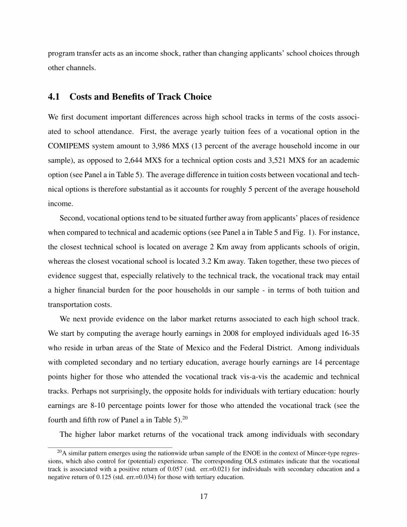
We first document important differences across high school tracks in terms of the costs associ-

ated to school attendance. First, the average yearly tuition fees of a vocational option in the

COMIPEMS system amount to 3,986 MX$ (13 percent of the average household income in our

sample), as opposed to 2,644 MX$ for a technical option costs and 3,521 MX$ for an academic

option (see Panel a in Table 5). The average difference in tuition costs between vocational and tech-

nical options is therefore substantial as it accounts for roughly 5 percent of the average household

income.

Second, vocational options tend to be situated further away from applicants’ places of residence

when compared to technical and academic options (see Panel a in Table 5 and Fig. 1). For instance,

the closest technical school is located on average 2 Km away from applicants schools of origin,

whereas the closest vocational school is located 3.2 Km away. Taken together, these two pieces of

evidence suggest that, especially relatively to the technical track, the vocational track may entail

a higher financial burden for the poor households in our sample - in terms of both tuition and

transportation costs.

We next provide evidence on the labor market returns associated to each high school track.

We start by computing the average hourly earnings in 2008 for employed individuals aged 16-35

who reside in urban areas of the State of Mexico and the Federal District. Among individuals

with completed secondary and no tertiary education, average hourly earnings are 14 percentage

points higher for those who attended the vocational track vis-a-vis the academic and technical

tracks. Perhaps not surprisingly, the opposite holds for individuals with tertiary education: hourly

earnings are 8-10 percentage points lower for those who attended the vocational track (see the

fourth and fifth row of Panel a in Table 5).20

The higher labor market returns of the vocational track among individuals with secondary

20A similar pattern emerges using the nationwide urban sample of the ENOE in the context of Mincer-type regres-sions, which also control for (potential) experience. The corresponding OLS estimates indicate that the vocationaltrack is associated with a positive return of 0.057 (std. err.=0.021) for individuals with secondary education and anegative return of 0.125 (std. err.=0.034) for those with tertiary education.

17

education observed in the labor survey data can affect individual preferences only to the extent

that COMIPEMS applicants can rely on this information. While we do not have information about

students’ expectations at the moment of the application, we can observe students’ expected returns

during the last year of high school, as measured by the Enlace de contexto. Students’ subjective

expectations about earnings five years after high school completion across the different high school

tracks in the metropolitan area of Mexico City are broadly consistent with the ENOE data (see

Figure 5).

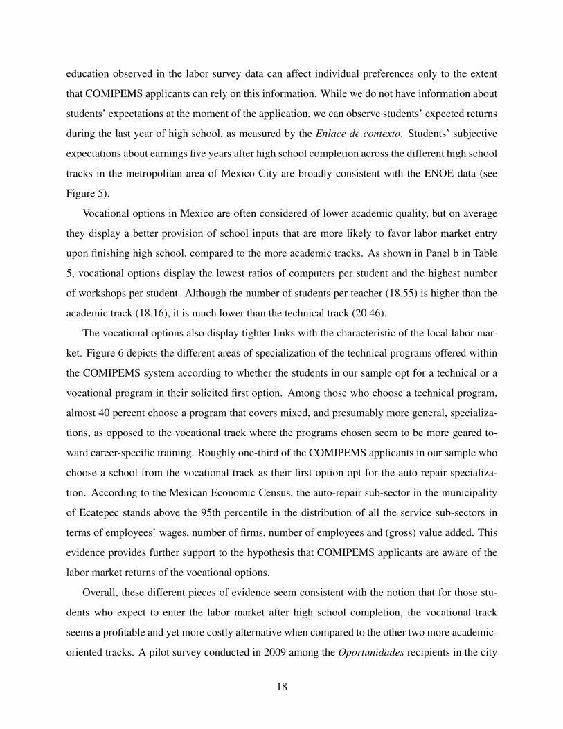
Vocational options in Mexico are often considered of lower academic quality, but on average

they display a better provision of school inputs that are more likely to favor labor market entry

upon finishing high school, compared to the more academic tracks. As shown in Panel b in Table

5, vocational options display the lowest ratios of computers per student and the highest number

of workshops per student. Although the number of students per teacher (18.55) is higher than the

academic track (18.16), it is much lower than the technical track (20.46).

The vocational options also display tighter links with the characteristic of the local labor mar-

ket. Figure 6 depicts the different areas of specialization of the technical programs offered within

the COMIPEMS system according to whether the students in our sample opt for a technical or a

vocational program in their solicited first option. Among those who choose a technical program,

almost 40 percent choose a program that covers mixed, and presumably more general, specializa-

tions, as opposed to the vocational track where the programs chosen seem to be more geared to-

ward career-specific training. Roughly one-third of the COMIPEMS applicants in our sample who

choose a school from the vocational track as their first option opt for the auto repair specializa-

tion. According to the Mexican Economic Census, the auto-repair sub-sector in the municipality

of Ecatepec stands above the 95th percentile in the distribution of all the service sub-sectors in

terms of employees’ wages, number of firms, number of employees and (gross) value added. This

evidence provides further support to the hypothesis that COMIPEMS applicants are aware of the

labor market returns of the vocational options.

Overall, these different pieces of evidence seem consistent with the notion that for those stu-

dents who expect to enter the labor market after high school completion, the vocational track

seems a profitable and yet more costly alternative when compared to the other two more academic-

oriented tracks. A pilot survey conducted in 2009 among the Oportunidades recipients in the city

18

of Ecatepec de Morelos provides some basic information on schooling expectations in our set-

ting. Among the 1,822 individuals aged 14-15, roughly 40 percent report secondary education as

the highest schooling level that they expect to complete. Hence, there is a potentially very large

fraction of high school entrants for whom the vocational track should be attractive. The size of

the potential demand for the vocational track helps to contextualize the large effect of the cash

transfers on track choices documented in Section 3.3.

4.2 Empirical Evidence

High-ability students are more likely to attend university, and hence they foresee the higher labor

market returns of an academic-oriented track. Those students are also more likely be less finan-

cially constrained due to higher access to merit-based scholarship at the upper secondary level.21

We thus expect Oportunidades to have a larger impact on high school track preferences among

lower ability students. We use information on the cumulative Grade Point Average (GPA) in lower

secondary and accordingly classify as high-ability and low-ability students whose GPA is above

and below the median respectively. We allow the ITT effect to vary with the level of ability and we

report the results in column 1 in Table 6. For those with a high GPA the effect of Oportunidades

on the probability of choosing the vocational track as first option is small and not statistically sig-

nificant from zero, as opposed to a large and statistically significant effect (5.7 percentage points)

for those with a GPA below the median.

Transportation costs may constrain school choices, especially in low income families. If Opor-

tunidades is changing preferences for high school tracks by relaxing the financial constraints, we

do expect the effect on the probability of choosing the vocational track to be stronger among those

applicants who live further away from a vocational option. We pull together the data on the entire

set of preferences of all the individuals in our sample and we consider this as the universe of the

high schools that students in our sample can potentially apply to. For each student in our sample,

we compute the distance from its residence address to the closest vocational option and we use this

as a proxy for the transportation cost that students have to sustain in order to attend a vocational

21For instance, students whose COMIPEMS score are high enough to enter UNAM options are provided with directaccess to university programs of the same institution - among the best ones in the country - and are automaticallygranted a scholarship that covers most of the school-related expenses both at secondary and tertiary level.

19

program. We study how the ITT effect on the probability of listing a vocational as first option varies

for low and high distance students, as defined by being below and above the median distance from

the closest Vocational option. The results are reported in column 4 in Table 6. The size of the

ITT coefficient is large (5 percentage point) and statistically significant for high-distance students,

while it is small and not statistically significant for low-distance students. Nevertheless, when we

test whether the two coefficients are statistically different, we cannot reject the null hypothesis of

no difference (p value=0.136).

If the eligibility for the cash transfer increases the propensity to choose the vocational track by

weakening the household financial constraints, then we would expect students to prefer more ex-

pensive - either in terms of tuition or transportation costs - options. For each option in the portfolio,

we thus construct the tuition cost and the distance from the applicants’ places of residence asso-

ciated with the school where the option is located.22 Roughly 30% of schooling options feature 0

tuition costs. Those refer mainly to “elite” schools belonging to sub-systems which are, by far, the

most demanded by relatively high-ability applicants (UNAM offers general education programs

while IPN administers technical education programs). By taking logs we automatically exclude

those schooling options and thus focus on the intensive margin of tuition fees. We then estimate

the ITT effect of the cash transfers on two outcomes: the logarithm of the tuition cost of the first

portfolio choice and the distance from students’ place of residence to the first choice. Results are

reported in Table 7. We find that the eligibility for Oportunidades significantly increases the tuition

cost associated with the preferred option in a range between 7.6% and 10.7%, depending on the

specification (columns 1-3). Looking at the effect of the cash transfer on the average willingness

to commute to the preferred school, we find a positive and significant impact of roughly 1.5 Km

(columns 5-6) - although this effect is not significant in the parametric specification (column 4).

The results presented in this section, although not conclusive, provide some evidence in support

of the financial constraints hypothesis. The probability of choosing the vocational track as first

option increases for those students who live further away and those with have lower scores in

the GPA. Consistently, we find that cash transfers have a positive impact on the tuition and the

transportation costs that students are willing to pay in order to attend their preferred schooling

22If two options within the same school have different tuition costs - e.g. due to the different types of materialsrequired, the outcome variable would be measured with error. Nevertheless, the measurement error is unlikely to bedifferent for options located above and below the eligibility threshold.

20

option.

4.3 Alternative Channels

As described in Section 2.2, Oportunidades transfers are conditional on health and schooling be-

haviors. Although there is no component of the transfer that is directly linked to the high school

track attended, we can not a priori rule out the possibility that our results are the outcome of the

conditional nature of the transfer. The requirements that each eligible child has to be enrolled in

school for receiving the scholarship component of the transfer and that she can not receive the

transfer more than twice for the same grade might have a direct effect on school choices. For in-

stance, students’ may strategically select relatively easier schools so as to increase their chances of

passing grades and receiving Oportunidades scholarships up until the end of upper secondary.

We use equation 2 to test whether the eligibility for the cash transfer had an impact on the

level of difficulty of the most preferred high school option in applicants’ portfolios. Under the

assumption that schools’ achievement standards partly depend on the student ability composition,

one plausibly good proxy measure for the degree of difficulty of a given schooling option is the

relative cutoff score in the admission exam due to the assignment algorithm of the COMIPEMS

system (see Section 2.1 for details). Regression results presented in columns 1-3 in Table 8 show

that, irrespective of the specification, the impact of the eligibility for the cash transfer on the

cutoff score of the first option requested in the COMIPEMS system is small and not statistically

significant from zero.

One potential concern with this measure is that it does not encompass the potential role of

schooling inputs and the different pedagogical methods on students’ (perceived) study effort and

probability of progressing through grades. We thus alternatively employ the school-average per-

formance among twelfth graders in a national standardized test aimed at measuring academic

achievement (ENLACE) in language and math as a broader measure of school difficulty, at the

cost of decreasing sample sizes due to missing average scores for roughly 30% of the high school

options in our sample. The estimates are reported in columns 4-9 of Table 8 and they consistently

reveal no effects of the eligibility for the Oportunidades scholarships. We interpret these results as

evidence that the results discussed in Section 3.3 are not the artifact of conditionalities’ compliance

21

among children in eligible households.23

5 Further Evidence

While the primary objective of our study is to understand how the Oportunidades transfer changed

student preferences over high school tracks, here we want to assess whether the observed changes

in preferences ultimately lead to better educational outcomes. Technical options display on average

lower tuition and transportation costs than the vocational ones, but they require higher scores to be

admitted. Therefore, more financially constrained students might de facto reduce the probability

of being assigned to their first option in the attempt to pursue a more affordable one. For this

purpose, we study whether the cash transfers increase the probability of being assigned to the first

option. Column 1 in Table 9 shows a 4 percentage point increase, but the effect is not statistically

significant. Final assignment depends both on student’s ranking and the score in the COMIPEMS

exam. Since the estimates reported in Table 4 do not show any effect on the exam, we treat

the COMIPEMS score as a plausibly exogenous variable. Including score fixed effects increases

the size of the coefficient but the effect, that corresponds to about 0.12 standard deviation of the

dependent variable, is not statistically significant (column 2). Yet, this effect is likely to vary with

the extent of the financial constraints, as measured by distance from students places of residence

to the closest vocational option. In fact, we find that the coefficient is larger and statistically

significant (at the 5% level) for students who live further away from schools offering vocational

programs (column 3).

By relaxing the financial constraints for some students, cash transfers are likely to improve the

allocation of students among school tracks, and this in turn should lead to better outcomes later

on. Because we lack individual-level data on graduation, taking a standardized achievement test

(ENLACE) in 12th grade is used as a proxy for graduation. Only students on track to graduate at

the end of the school year are registered to take the exam. Previous studies [De Janvry et al., 2013;

Estrada and Gignoux, 2014] present evidence that this is a good proxy, in particular because there

is no evidence that schools administer the exam strategically. On average, 44% of the students in

23As an additional test, we use the school-level June pass rates in the academic year 2005-2006 in order to furthercorroborate that students above the eligibility threshold do not prefer easier schooling options. Results (available uponrequest) are consistent with the estimates reported in Table 8.

22

our sample take this exam, and only 8% of them do so from the vocational track. We thus study

whether the eligibility to Oportunidades increases the probability of high school completion in the

vocational track. The estimation results which are displayed in columns 4 and 5 of Table 9 show

a positive but not statistically significant effect in the entire sample. Again, we a find larger and

statistically significant effect (at the 10% level) when we focus on those students who are more

financially constrained, as measured by their distance to the closest school offering a vocation

program (column 6).

Most of the results presented in this section are not statistically significant at the conventional

level and this might be arguably related to the limited number of observations in our sample.

Beyond school choice decisions, there may be other channels through which Oportunidades can

affect medium-term academic trajectories. Nevertheless, taken together, this evidence is suggestive

that cash transfers, by relaxing the financial constraints that prevent low-income students from

attending a vocational school, may have persistent impacts on both school placement and later

academic trajectories.

6 Conclusions

There is little systematic evidence on the factors underlying students’ (and parents’) demand for

the different educational modalities. Especially in developing countries, financial constraints can

induce students from disadvantaged backgrounds to opt for school options that do not match either

with their skills or their career expectations. In this paper, we have explored the extent to which

differences in costs and benefits across high school tracks affect school choice decisions within a

high-stake assignment mechanism in the metropolitan area of Mexico City.

Quasi-experimental evidence which exploited the discontinuity in the eligibility for the cash

transfer program Oportunidades documented that the receipt of an income shock increases by

6.1 percentage points the probability of choosing the vocational track for the sub-population of

students in the neighborhood of the program eligibility cutoff. Although this is by construction a

local effect that is difficult to extrapolate to other segments of the population of applicants in this

context, it draws on a policy-relevant segment of low-income students in an urban setting of a large

developing country.

23

Consistent with a simple school choice model with financial constraints, this effect is more

pronounced among students who are more likely to reap the higher returns from a vocational

education and those who have higher costs in accessing the associated school facilities. Among

the latter group, we have also shown that these short-run responses to the cash transfer can translate

into better academic trajectories in high school. These findings reveal the presence of an untapped

demand for vocational education which is hindered by credit market imperfections. In this sense,

demand-side subsidies which partly cover tuition and/or transportation costs (e.g. school vouchers)

may be effective policy tools to increase enrollment in vocational education at the secondary level.

24

References

Ajayi, K. [2013], School Choice and Educational Mobility: Lessons from Secondary School Ap-

plications in Ghana, mimeo, Boston University - Department of Economics.

Angelucci, M. [forthcoming], ‘Migration and financial constraints: Evidence from Mexico’, Re-

view of Economics and Statistics .

Angelucci, M. and Attanasio, O. [2009], ‘Oportunidades: Program Effect on Consumption,

Low Participation, and Methodological Issues’, Economic Development and Cultural Change

57(3), 479–506.

Angelucci, M. and Attanasio, O. [2013], ‘The Demand for Food of Poor Urban Mexican House-

holds: Understanding Policy Impacts Using Structural Models’, American Economic Journal:

Economic Policy 5(1), 146–78.

Arcidiacono, P. [2004], ‘Ability sorting and the returns to college major’, Journal of Econometrics

121(1-2), 343–375.

Arcidiacono, P. [2005], ‘Affirmative Action in Higher Education: How do Admission and Financial

Aid Rules Affect Future Earnings?’, Econometrica 73(5), 1477–1524.

Attanasio, O. and Kaufmann, K. [forthcoming], ‘Education Choices and Returns to Schooling: In-

trahousehold Decision Making, Gender and Subjective Expectations.’, Journal of Development

Economics .

Avery, C. and Hoxby, C. [2012], The Missing “One-Offs”: The Hidden Supply of High Achieving,

Low Income Students. NBER Working paper No. 18586.

Bettinger, E. P., Long, B. T., Oreopoulos, P. and Sanbonmatsu, L. [2012], ‘The Role of Appli-

cation Assistance and Information in College Decisions: Results from the H&R Block Fafsa

Experiment’, The Quarterly Journal of Economics 127(3), 1205–1242.

Betts, J. R. [2011], The Economics of Tracking in Education, Vol. 3 of Handbook of the Economics

of Education, Elsevier, chapter 7, pp. 341–381.

25

Bobba, M. and Frisancho, V. [2014], Learning About Oneself: The Effects of Signaling Academic

Ability on School Choice. Working Paper.

Burgess, S., Greaves, E., Vignoles, A. and Wilson, D. [2009], What Parents Want: School prefer-

ences and school choice, The Centre for Market and Public Organisation 09/222, Department of

Economics, University of Bristol, UK.

De Janvry, A., Dustan, A. and Sadoulet, E. [2013], Flourish or Fail? The Risky Reward of Elite

High School Admission in Mexico City. Working Paper.

Deming, D. J., Hastings, J. S., Kane, T. J. and Staiger, D. O. [2014], ‘School Choice, School

Quality, and Postsecondary Attainment’, American Economic Review 104(3), 991–1013.

Dinkelman, T. and Martinez, C. [2014], ‘Investing in Schooling In Chile: The Role of Information

about Financial Aid for Higher Education’, The Review of Economics and Statistics 96(2), 244–

257.

Dustan, A. [2014], Peer Networks and School Choice under Incomplete Information. Working

Paper.

Dustmann, C., Puhani, P. A. and Schönberg, U. [2014], The Long-Term Effects of Early Track

Choice, IZA Discussion Papers 7897, Institute for the Study of Labor (IZA).

Estrada, R. and Gignoux, J. [2014], Benefits to elite schools and the formation of expected returns

to education: Evidence from Mexico City. Working Paper.

Giustinelli, P. [2014], Group Decision Making with Uncertain Outcomes: Unpacking Child-Parent

Choice of the High School Track, mimeo, University of Michigan - Department of Economics.

Gonzalez-Flores, M., Heracleous, M. and Winters, P. [2012], ‘Leaving the Safety Net: An

Analysis of Dropouts in an Urban Conditional Cash Transfer Program’, World Development

40(12), 2505–2521.

Hastings, J., Kane, T. and Staiger, D. [2008], Heterogeneous preferences and the efficacy of public

school choice. Combines and replaces National Bureau of Economic Research Working Papers

No. 12145 and 11805.

26

Hastings, J. S. and Weinstein, J. M. [2008], ‘Information, School Choice, and Academic Achieve-

ment: Evidence from Two Experiments’, The Quarterly Journal of Economics 123(4), 1373–

1414.

Hoddinott, J. and Skoufias, E. [2004], ‘The Impact of PROGRESA on Food Consumption’, Eco-

nomic Development and Cultural Change 53(1), 37–61.

Imbens, G. and Kalyanaraman, K. [2012], ‘Optimal Bandwidth Choice for the Regression Discon-

tinuity Estimator’, Review of Economic Studies 79(3), 933–959.

Jensen, R. [2010], ‘The (Perceived) Returns to Education and The Demand for Schooling’, Quar-

terly Journal of Economics 125(2), 515–548.

Kaufmann, K. [forthcoming], ‘Understanding the Income Gradient in College Attendance in Mex-

ico: The Role of Heterogeneity in Expected Returns’, Quantitative Economics .

Kerr, S. P., Pekkarinen, T. and Uusitalo, R. [2013], ‘School Tracking and Development of Cogni-

tive Skills’, Journal of Labor Economics 31(3), 577 – 602.

Lai, F., Sadoulet, E. and de Janvry, A. [2009], ‘The Adverse Effects of Parents’ School Selec-

tion Errors on Academic Achievement: Evidence from the Beijing Open Enrollment Program’,

Economics of Education Review 28(4), 485–496.

Lee, D. S. [2008], ‘Randomized experiments from non-random selection in U.S. House elections’,

Journal of Econometrics 142(2), 675–697.

Lee, D. S. and Lemieux, T. [2010], ‘Regression Discontinuity Designs in Economics’, Journal of

Economic Literature 48(2), 281–355.

Lochner, L. and Monge-Naranjo, A. [2012], ‘Credit Constraints in Education’, Annual Review of

Economics 4, 225–256.

Martinelli, C. and Parker, S. W. [2009], ‘Deception and misreporting in a social program’, Journal

of the European Economic Association 7(4), 886–908.

McCrary, J. [2008], ‘Manipulation of the running variable in the regression discontinuity design:

A density test’, Journal of Econometrics 142(2), 698–714.

27

Mizala, A. and Urquiola, M. [2013], ‘School markets: The impact of information approximating

schools’ effectiveness’, Journal of Development Economics 103(C), 313–335.

Pathak, P. [2011], ‘The Mechanism Design Approach to Student Assignment’, Annual Review of

Economics, Annual Reviews 3(1), 513–536.

Skoufias, E., Davis, B. and de la Vega, S. [2001], ‘Targeting the Poor in Mexico: An Evaluation of

the Selection of Households into PROGRESA’, World Development 29(10), 1769–1784.

Wiswall, M. and Zafar, B. [forthcoming], ‘Determinants of college major choice: Identiöcation

using an information experiment’, The Review of Economic Studies. .

28

Figures

Figure 1: The Geographic Distribution of COMIPEMS Options

!(

!(

!(!(

!(

!(

!(

!(

!(

!(

!(

!(

!(

!(

!(

!(

!(

!(

!(

!(

!(

!(

!(

!(

!(!(!(

!(

!(

!(

!(

!(

!(

!(

!(

!(

!(

!(

!(

!(

!(

!(

!(

!(

!(

!(

!(

!(

!(

!(

!(

!(

!(

!(

!(

!(

!(

!(!(!(

!(

!(

!(

!(

!(

!(

!(

!(

!(!(

!(

!(

!(

!(

!(

!(

!(

!(

!(

!(

!(

!(

!(

!(

!(

!(

!(

!(!(

!(!(

!(!(

!(

!(

!(

!(

!(

!(

!(

!(

!( !(

!(

!(

!(

!(

!(

!(

!(

!(

!(

!(

!(

!(

!(

!(!(

!(

!(

!(

!(

!(

!(

!(

!(

!(

!(

!(

!(

!(

!(

!(

!(

!(

!(

!(!(

!(

!(

!(

!(!(

!(

!(

!(

!(

!(

!(

!(

!(

!(

!(

!(

!(

!(

!(

!(

!(

!(

!(

!(

!(

!(

!(

!(

!(

!(

!(

!(

!(

!(!(

!(

!(

!(

!(

!(

!(

!(

!(

!(

!(

!(

!(

!(

!(

!(

!(

!(

!(

!(

!(

!(

!(

!(

!(

!(

!(

!(

!(

!(

!( !(

!(

!(

!(

!(

!(

!(

!(

!(

!(

!(

!(

!(

!(

!(

!(

!(

!(

!(

!(

!(

!(

!(

!(

!(

!(

!(

!(!(

!(

!(

!(

!(

!(

!(

!(

!(

!(

!(

!(

!(

!(

!(

!(

!( !(

!(

!(

!(

!(

!(

!(

!(

!(

!(

!(

!(

!(

!(

!(

!(

!(

!(

!(

!(

!(

!(

!(

!(

!(

!(

!(

!(

!(

!(

!(

!(

!(

!(

!(

!(

!(

!(!(

!(

!(

!(

!(

!(

!(

!(

!(

!(

!(

!(

!(

!(

!(

!(

!(

!(

!(

!(

!(

#

#

#

#

##

# #

#

##

#

#

#

#

#

#

#

#

#

#

##

#

#

#

##

#

#

#

#

#

#

#

#

##

##

#

#

# #

#

#

#

#

#

#

#

##

#

#

#

#

#

# #

#

##

#

##

#

#

#

#

#

#

#

#

#

#

#

#

#

#

#

#

#

#

#

#

#

#

#

#

#

##

##

#

#

#

#

##

#

#

#

#

#

#

#

#

##

#

##

#

#

#

#

#

#

#

##

#

#

#

###

#

#

#

#

#

##

#

# #

#

#

#

#

##

#

#

##

#

#

#

##

#

#

#

#

#

#

#

#

#

#

#

#

#

#

#

#

#

#

#

#

#

#

###

#

#

#

#

#

#

#

#

#

#

#

#

#

#

#

##

#

#

#

# #

#

#

#

#

##

##

##

#

#

#

#

#

#

#

#

#

#

#

#

#

#

#

#

###

#

#

#

#

VocationalAcademic trackTechnical track

0 10 205 Kilometers

0 4 82 Kilometers

# Middle schools for COMIPEMS applicants

NOTE: This map reports the geographic locations of the schooling options that participate to the COMIPEMS as-signment system during the period 2005-2010. The quadrant in the up-right corner displays a close-up view of theMunicipality of Ecatepec in which the markers reflect the locations of the middle-schools of origin for the applicantsin our sample.

29

Figure 2: Density of the Program Eligibility Score

0.1

.2.3

.4.5

Freq

uenc

y

-2 0 2 4Distance from the Eligibility Cutoff

NOTE: This figure depicts a kernel regression interpolation along with the confidence intervals of the empirical distri-bution of the assignment variable at the points below and above the cutoff. The bin size and the optimal bandwidth arecalculated using the procedure described in McCrary [2008].

30

Figure 3: Continuity Tests for Covariates

15.3

15.4

15.5

15.6

Smoo

th A

vera

ge

-1 -.5 0 .5 1Distance from the Eligibility Cutoff

(a) Age

.02

.04

.06

.08

.1.1

2Sm

ooth

Ave

rage


(b) Ethnicity (indigenous)

2.8

33.

23.

43.

6Sm

ooth

Ave

rage


(c) Household Monthly Income (categorical)

3.6

3.8

44.

24.

44.

6Sm

ooth

Ave

rage


(d) Parental Education (categorical)

22.

53

3.5

Smoo

th A

vera

ge


(e) Number of Siblings

.02

.04

.06

.08

.1.1

2Sm

ooth

Ave

rage


(f) Live with Both Parents

NOTE: Circles represent sample averages of the dependent variable computed on 0.10 point brackets of the runningvariable. The solid line (dashed line) is a local linear regression prediction (least squares running-mean smoothing),separated on either side of the threshold. For presentational reasons, the figure plots averages of the dependent variablewith values of the running variable comprised between -1 and 1. The red vertical line denotes the discontinuity,normalized to zero.

31

Figure 4: Discontinuity Effects of Program Eligibility on Track Choice

0.2

.4.6

.81

Smoo

th A

vera

ge


(a) Program Take-up0

.05

.1.1

5Sm

ooth

Ave

rage


(b) Vocational Track (1st option)

.35

.4.4

5.5

.55

Smoo

th A

vera

ge


(c) Technical Track (1st option)

.4.4

5.5

.55

.6Sm

ooth

Ave

rage


(d) Academic Track (1st option)

NOTE: Circles represent sample averages of the dependent variable computed on 0.10 point brackets of the runningvariable. The solid line (dashed line) is a local linear regression prediction (least squares running-mean smoothing),separated on either side of the threshold. For presentational reasons, the figure plots averages of the dependent variablewith values of the running variable comprised between -1 and 1. The red vertical line denotes the discontinuity,normalized to zero.

32

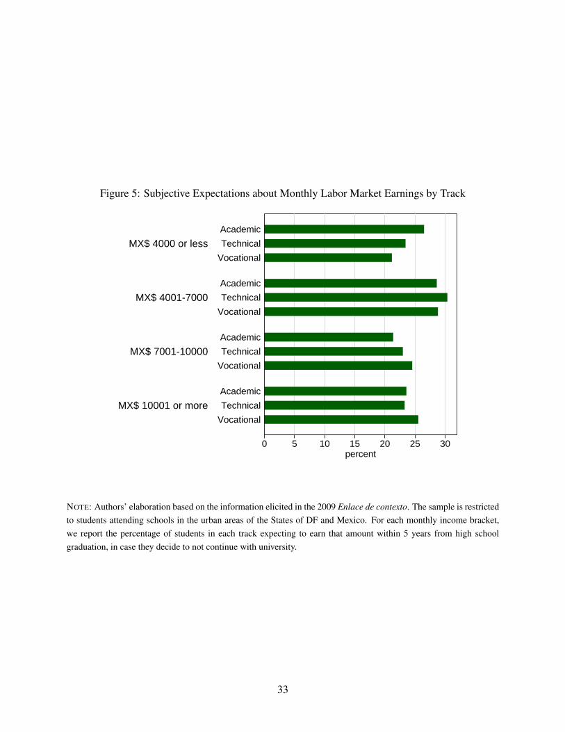
Figure 5: Subjective Expectations about Monthly Labor Market Earnings by Track

0 5 10 15 20 25 30percent

MX$ 10001 or more

MX$ 7001-10000

MX$ 4001-7000

MX$ 4000 or less

Vocational

Technical

Academic

Vocational

Technical

Academic

Vocational

Technical

Academic

Vocational

Technical

Academic

NOTE: Authors’ elaboration based on the information elicited in the 2009 Enlace de contexto. The sample is restrictedto students attending schools in the urban areas of the States of DF and Mexico. For each monthly income bracket,we report the percentage of students in each track expecting to earn that amount within 5 years from high schoolgraduation, in case they decide to not continue with university.

33

Figure 6: Type of Preferred Technical Program (1st Option) by Track

0.2

.4.6

.81

Vocational Technical track

Maintenance Information technologyElectronics Production processAccounting and Administration Health/SocialTourism/Cosmetology Mixed specializations

34

Tables

Table 1: Shares of Upper-Secondary Enrollment in a selected group of Countries

General Pre-vocational VocationalArgentina 82% 18%Brazil 86% 14%Chile 67% 33%Mexico 91% 9%

OECD average 54% 2% 44%

NOTE: Authors’ elaboration based on Education at a Glance 2011: OECD Indicators, OECD, Paris.

Table 2: Effect of the Oportunidades Transfer on Track Choices (1st option)

Outcome Variable Vocational General TechnicalParameter OLS-ITT IV-LATE OLS-ITT IV-LATE OLS-ITT IV-LATE

(1) (2) (3) (4) (5) (6)

Treat 0.040** 0.011 -0.051(0.019) (0.037) (0.036)

Take-up 0.061** 0.017 -0.079(0.03) (0.056) (0.056)

Mean Dep. Var. 0.092 0.465 0.443SD Dep. Var. 0.289 0.499 0.497Observations 5232 5232 5232 5232 5232 5232Clusters 2907 2907 2907 2907 2907 2907

NOTE: * significant at 10%; ** significant at 5%; *** significant at 1%.OLS estimates (quadratic spline specification for the eligibility score). Standard errors clustered by valuesof the eligibility score in parenthesis. The dummy variable Vocational/General/Technical takes the value 1if a Vocational/General/Technical option is listed first in the applicant’s portfolio.

35

Table 3: Alternative Specifications for the ITT Estimates

Outcome Variable Vocational General TechnicalEstimator LLR-Kernel LLR-Kernel LLR-Kernel

Triang. Rectang. Triang. Rectang. Triang. Rectang.(1) (2) (3) (4) (5) (6)

Treat 0.046** 0.049** 0.012 -0.001 -0.065 -0.051(0.020) (0.020) (0.043) (0.043) (0.045) (0.046)

Mean Dep. Var. 0.092 0.465 0.443SD Dep. Var. 0.289 0.499 0.497Observations 3908 3240 3143 2578 2792 2245Clusters 2093 1727 1670 1346 1468 1159

NOTE: * significant at 10%; ** significant at 5%; *** significant at 1%.Local Linear Regression estimates using the optimal bandwidth criterion in Imbens and Kalya-naraman [2012]. Standard errors clustered by values of the eligibility score in parenthesis. Thedummy variable Vocational/General/Technical takes the value 1 if a Vocational/General/Technicaloption is listed first in the applicant’s portfolio.

Table 4: Test for compositional changes

Outcome Variable COMIPEMS (Y/N) Comipems Score GPA(1) (2) (3)

Treat -0.003 -0.943 -0.248(0.017) (1.298) (0.173)

Mean Dep. Var. 0.244 57.745 7.352SD Dep. Var. 0.429 17.584 2.434Observations 21463 5059 5232Clusters 6138 2856 2907

NOTE: OLS estimates (quadratic spline specification for the eligibility score).Standard errors clustered by values of the eligibility score in parenthesis. Thedummy COMIPEMS takes the value 1 if the individual took part in theCOMIPEMS application process, 0 otherwise. The COMIPEMS score is the resultof a standardized exam that consists of 128 multiple choice questions. The GPAscore reflects results in lower-secondary and varies in the range between 0 and 10.

36

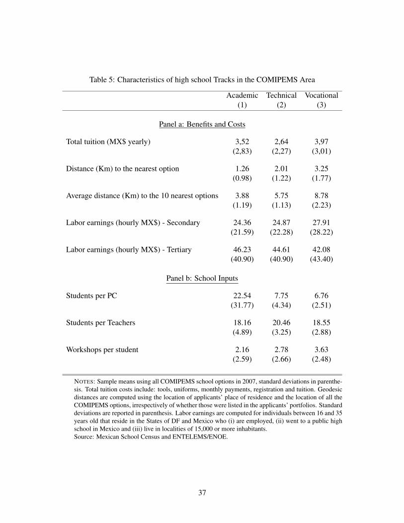
Table 5: Characteristics of high school Tracks in the COMIPEMS Area

Academic Technical Vocational(1) (2) (3)

Panel a: Benefits and Costs

Total tuition (MX$ yearly) 3,52 2,64 3,97(2,83) (2,27) (3,01)

Distance (Km) to the nearest option 1.26 2.01 3.25(0.98) (1.22) (1.77)

Average distance (Km) to the 10 nearest options 3.88 5.75 8.78(1.19) (1.13) (2.23)

Labor earnings (hourly MX$) - Secondary 24.36 24.87 27.91(21.59) (22.28) (28.22)

Labor earnings (hourly MX$) - Tertiary 46.23 44.61 42.08(40.90) (40.90) (43.40)

Panel b: School Inputs

Students per PC 22.54 7.75 6.76(31.77) (4.34) (2.51)

Students per Teachers 18.16 20.46 18.55(4.89) (3.25) (2.88)

Workshops per student 2.16 2.78 3.63(2.59) (2.66) (2.48)

NOTES: Sample means using all COMIPEMS school options in 2007, standard deviations in parenthe-sis. Total tuition costs include: tools, uniforms, monthly payments, registration and tuition. Geodesicdistances are computed using the location of applicants’ place of residence and the location of all theCOMIPEMS options, irrespectively of whether those were listed in the applicants’ portfolios. Standarddeviations are reported in parenthesis. Labor earnings are computed for individuals between 16 and 35years old that reside in the States of DF and Mexico who (i) are employed, (ii) went to a public highschool in Mexico and (iii) live in localities of 15,000 or more inhabitants.Source: Mexican School Census and ENTELEMS/ENOE.

37

Table 6: Treatment Heterogeneity: ITT on the Probability of Choos-ing Vocational as 1st Choice

by GPA by Distance(1) (2)

Treat X Low GPA 0.057***(0.021)

Treat X High GPA 0.026(0.020)

Treat X Low Dist 0.025(0.021)

Treat X High Dist 0.050**(0.022)

P value H0: Treat X Low=treatX High 0.056 0.134

Mean Dep. Var. 7.352 3.247SD Dep. Var. 2.434 1.773Observations 5232 4893Clusters 2907 2803

NOTE: * significant at 10%; ** significant at 5%; *** significant at 1%.OLS estimates (quadratic spline specification for the eligibility score). Stan-dard errors clustered by values of the eligibility score in parenthesis. Equa-tion 2 has been estimated allowing for the interaction between the treatmentdummy and the dummies for Low and High GPA (column 1) as well asLow and High Distance (column 2). A student is classified as Low(High)GPA if she scored below(above) the median GPA. A student is classified asLow(High) Distance if the distance between her residence and the closestVocational option in the entire set of available options is below(above) themedian geodesic distance.

38

Table 7: ITT Effects on the Costs of the 1st Choice

Outcome Variable Log Total Tuition Fees Distance from Residence (Km)Estimator Quadratic LLR LLR Quadratic LLR LLR

Spline Triang. Rectang. Spline Triang. Rectang.(1) (2) (3) (4) (5) (6)

Treat 0.076* 0.090* 0.107** 0.559 1.490** 1.633**(0.045) (0.049) (0.050) (0.476) (0.718) (0.714)

Mean Dep. Var. 7.993 7.979 7.973 8.242 8.379 8.311SD Dep. Var. 0.524 0.527 0.528 6.205 6.178 6.205Observations 3507 2120 1738 4756 1867 1497Clusters 2245 1320 1075 2768 1007 806

NOTE: * significant at 10%; ** significant at 5%; *** significant at 1%.Standard errors clustered by values of the eligibility score in parenthesis. Total tuition costs fees:tools, uniforms, monthly payments, registration and tuition. The geodesic distance is computed usingthe location of applicants’ place of residence and the location of the 1st option.

39

Tabl

e8:

Scho

olSe

lect

ivity

ofth

e1s

tCho

ice

Dep

ende

ntV

aria

ble

Adm

issi

onC

utof

fE

MS

Span

ish

EM

SM

ath

Est

imat

orQ

uadr

atic

LL

RL

LR

Qua

drat

icL

LR

LL

RQ

uadr

atic

LL

RL

LR

Splin

eTr

iang

.R

ecta

ng.

Splin

eTr

iang

.R

ecta

ng.

Splin

eTr

iang

.R

ecta

ng.

(1)

(2)

(3)

(4)

(5)

(6)

(7)

(8)

(9)

Trea

t-0

.954

-0.6

41-0

.548

-0.0

21-0

.051

-0.0

38-0

.023

-0.0

45-0

.034

(1.5

19)

(1.5

23)

(1.5

47)

(0.0

43)

(0.0

47)

(0.0

48)

(0.0

57)

(0.0

58)

(0.0

60)

Mea

nD

ep.V

ar.

67.9

960.

372

0.41

3SD

Dep

.Var

.20

.330

0.52

20.

694

Obs

erva

tions

5143

3939

3305

3792

2480

2054

3792

2807

2309

Clu

ster

s28

7521

3317

7723

8615

2212

3823

8617

2114

14

NO

TE

:*si

gnifi

cant

at10

%;*

*si

gnifi

cant

at5%

;***

sign

ifica

ntat

1%.S

tand

ard

erro

rscl

uste

red

byva

lues

ofth

eel

igib

ility

scor

ein

pare

nthe

sis.

Adm

issi

onC

utof

fis

the

low

estC

OM

IPE

MS

scor

eam

ong

stud

ents

adm

itted

toth

eop

tion

liste

das

first

.E

MS

Span

ish

and

Mat

hre

pres

entt

he20

08sc

hool

aver

age

12th

grad

eE

NL

AC

Ein

Mat

han

dSp

anis

h

40

Tabl

e9:

Plac

emen

tOut

com

esan

dM

ediu

m-T

erm

Out

com

es

Dep

ende

ntV

aria

ble

Ass

ignm

entt

oth

e1s

tCho

ice

(Y/N

)E

NL

AC

E12

thgr

ade

inVo

catio

nal(

Y/N

)(1

)(2

)(3

)(4

)(5

)(6

)

Trea

t0.

040

0.05

30.

010

0.00

8(0

.038

)(0

.036

)(0

.020

)(0

.021

)Tr

eatX

Low

Dis

tanc

e0.

043

0.00

4(0

.040

)(0

.021

)Tr

eatX

Hig

hD

ista

nce

0.08

1**

0.03

8*(0

.041

)(0

.021

)

CO

MIP

EM

Ssc

ore

deci

les

fixed

effe

cts

No

Yes

Yes

No

Yes

Yes

Pva

lueH

0:T

reat

XL

ow=T

reat

XH

igh

0.19

90.

045

Mea

nD

ep.V

ar.

0.37

20.

372

0.37

50.

080

0.08

20.

082

SDD

ep.V

ar.

0.48

30.

483

0.48

40.

271

0.27

50.

274

Obs

erva

tions

4234

4234

3940

5232

5059

4726

Clu

ster

s25

9225

9224

8829

0728

5627

52

NO

TE

:*si

gnifi

cant

at10

%;*

*si

gnifi

cant

at5%

;***

sign

ifica

ntat

1%.

OL

Ses

timat

es(q

uadr

atic

splin

esp

ecifi

catio

nfo

rth

eel

igib

ility

scor

e).

Stan

dard

erro

rscl

uste

red

byva

lues

ofth

eel

igib

ility

scor

ein

pare

nthe

sis.

The

dum

my

Ass

ignm

entt

oth

e1s

tCho

ice

take

sth

eva

lue

1if

the

stud

enti

sas

sign

edto

the

first

optio

nlis

ted

inth

epo

rtfo

lio,0

othe

rwis

e.

41

Documents

High School Track Choice and Financial Constraints