LUND UNIVERSITY

PO Box 117221 00 Lund+46 46-222 00 00

High resolution time-frequency representations

Reinhold, Isabella

2017

Document Version:Annan version

Link to publication

Citation for published version (APA):Reinhold, I. (2017). High resolution time-frequency representations. Lund University / Centre for MathematicalSciences /LTH.

General rightsUnless other specific re-use rights are stated the following general rights apply:Copyright and moral rights for the publications made accessible in the public portal are retained by the authorsand/or other copyright owners and it is a condition of accessing publications that users recognise and abide by thelegal requirements associated with these rights. • Users may download and print one copy of any publication from the public portal for the purpose of private studyor research. • You may not further distribute the material or use it for any profit-making activity or commercial gain • You may freely distribute the URL identifying the publication in the public portal

Read more about Creative commons licenses: https://creativecommons.org/licenses/Take down policyIf you believe that this document breaches copyright please contact us providing details, and we will removeaccess to the work immediately and investigate your claim.

HIGH RESOLUTION TIME-FREQUENCYREPRESENTATIONS

by

ISABELLA REINHOLD

Thesis for the degree of Licentiate of EngineeringTo be presented, with the permission of the Faculty of Engineering

at Lund University, for public criticism in room MH:309A,Mattehuset, Solvegatan 18, Lund, on Tuesday, the 28th of

November 2017 at 13:15 (1.15pm).

Faculty opponent: Prof. Sven Nordebo,Department of Physics and Electrical Engineering,

Linnaeus University, Sweden.

HIGH RESOLUTION TIME-FREQUENCYREPRESENTATIONS

ISABELLA REINHOLD

Faculty of EngineeringCentre for Mathematical Sciences

Mathematical Statistics

Public defenceNovember 28th, 2017, 13:15 in MH:309A, Centre for Mathematical Sciences, Lund University.Solvegatan 18, 223 62 Lund, Sweden.

AdvisorsProf. Maria Sandsten,Mathematical Statistics, Centre for Mathematical Sciences, Lund University, Sweden.Assoc. Prof. Josefin Starkhammar,Department of Biomedical Engineering, Lund University, Sweden.

Faculty opponentProf. Sven Nordebo,Department of Physics and Electrical Engineering,Linnaeus University, Sweden.

Mathematical StatisticsCentre for Mathematical SciencesLund UniversityBox 118SE–221 00 LundSweden

http://www.maths.lu.se/

Licentiate Theses in Mathematical Sciences 2017:2ISSN: 1404-028XISRN: LUTFMS-2019-2017

c© Isabella Reinhold 2017

Printed in Sweden by Media-Tryck, Lund University, Lund 2017

To everyone who has given me free coffee

Contents

List of publications . . . . . . . . . . . . . . . . . . . . . . . . . . . iiiAcknowledgements . . . . . . . . . . . . . . . . . . . . . . . . . . . vAbstract . . . . . . . . . . . . . . . . . . . . . . . . . . . . . . . . viPopular summary in English . . . . . . . . . . . . . . . . . . . . . . viiPopularvetenskaplig sammanfattning pa svenska . . . . . . . . . . . . ixSummary of notations . . . . . . . . . . . . . . . . . . . . . . . . . xi

High resolution time-frequency representations 11 The need for time-frequency analysis . . . . . . . . . . . . . . 12 Fundamental ideas for joint time-frequency

representations . . . . . . . . . . . . . . . . . . . . . . . . . . 53 Spectrogram and quadratic time-frequency

distributions . . . . . . . . . . . . . . . . . . . . . . . . . . . 114 Resolution and localisation . . . . . . . . . . . . . . . . . . . 155 Main results of the research papers . . . . . . . . . . . . . . . . 22

Scientific publications 31Author contributions . . . . . . . . . . . . . . . . . . . . . . . . . . 31

Paper A: Optimal time–frequency distributions using a novel signaladaptive method for automatic component detection 331 Introduction . . . . . . . . . . . . . . . . . . . . . . . . . . . 362 Time-frequency methods . . . . . . . . . . . . . . . . . . . . 383 Performance measure and a novel signal adaptive

method for automatic detection of auto-terms . . . . . . . . . . 404 Detection of auto-terms . . . . . . . . . . . . . . . . . . . . . 475 Optimal parameter estimation of kernels for HRV

signals . . . . . . . . . . . . . . . . . . . . . . . . . . . . . . 546 Discussion . . . . . . . . . . . . . . . . . . . . . . . . . . . . 567 Conclusion . . . . . . . . . . . . . . . . . . . . . . . . . . . 57

Paper B: Objective detection and time-frequency localization of com-ponents within transient signals 631 Introduction . . . . . . . . . . . . . . . . . . . . . . . . . . . 662 The reassigned spectrogram for transient signals . . . . . . . . . 683 Automatic component detection algorithm . . . . . . . . . . . 724 Resolution of the reassigned spectrogram for transient signals . . 755 Performance of the automatic component detection

algorithm . . . . . . . . . . . . . . . . . . . . . . . . . . . . 836 Examples on measured data . . . . . . . . . . . . . . . . . . . 867 Conclusions . . . . . . . . . . . . . . . . . . . . . . . . . . . 90

Paper C: The scaled reassigned spectrogram adapted for detection andlocalisation of transient signals 991 Introduction . . . . . . . . . . . . . . . . . . . . . . . . . . . 1022 The scaled reassigned spectrogram . . . . . . . . . . . . . . . . 1033 Simulations . . . . . . . . . . . . . . . . . . . . . . . . . . . 1094 Transient echolocation signal example . . . . . . . . . . . . . . 1125 Conclusions . . . . . . . . . . . . . . . . . . . . . . . . . . . 114

ii

List of publications

This thesis is based on the following publications:

A Optimal time–frequency distributions using a novel signal adaptivemethod for automatic component detection

Isabella Reinhold, Maria Sandsten.Signal Processing, Vol. 133, 250-259, 2017.

B Objective detection and time-frequency localization of componentswithin transient signals

Isabella Reinhold, Maria Sandsten, Josefin Starkhammar.Submitted to J. Acoust. Soc. Am.

C The scaled reassigned spectrogram adapted for detection and localisa-tion of transient signals

Isabella Reinhold, Josefin Starkhammar, Maria Sandsten.25th European Signal Processing Conference (EUSIPCO), 937-941, 2017.

Publications not included in this thesis:

1 Quality of academic writing for engineering students at Lund Univer-sity

Isabella Reinhold, Kenneth Batstone, Isabel M. Gallardo Gonzalez, AndreaTroian, Rixin Yu.The 2nd EuroSoTL conference, 2017.

2 Automatic time-frequency analysis of echolocation signals using thematched Gaussian multitaper spectrogram

Maria Sandsten, Isabella Reinhold, Josefin Starkhammar.Interspeech 2017, 3048-3052, 2017.

iii

3 A novel Doppler penalty function for the multitaper Wigner-Ville dis-tribution

Isabella Reinhold, Maria Sandsten.11th IMA International Conference on Mathematics in Signal Processing,2016.

4 Intra-click time-frequency patterns across the echolocation beam of abeluga whale

Josefin Starkhammar, Isabella Reinhold, Patrick Moore, Dorian Houser,Maria Sandsten.J. Acoust. Soc. Am., Vol. 140 (4), 3239, 2016.

iv

Acknowledgements

I wish to express my sincere thanks to my supervisor Maria Sandsten for her sup-port and guidance during these two years. I would also like to thank my assistantsupervisor Josefin Starkhammar, who have introduced interesting applications formy work. A heartfelt thanks also to the present and previous administrative andtechnical staff at the mathematical statistics department for their help in prac-tical matters. Thanks also to Rachele, who has shared the stress of simultaneouslyteaching and writing a thesis. Lastly, thanks to my parents Jeanette and Kent, mywonderful boyfriend Oskar, my brother Viktor, my first roommate Ase and all myfriends for always being there in times of need.

Isabella Reinhold

v

Abstract

Non-stationary signals are very common in nature, e.g. sound waves such ashuman speech, bird song and music. It is usually meaningful to describe a signalin terms of time and frequency. Methods for doing so exist and are well defined.From the time representation it is possible to see the oscillations or waves of thesignal and if the signal changes over time. From the frequency representation,obtained from the Fourier transform, the frequency decomposition of the signalcan be seen, i.e. which frequencies the signal contains.

However the time and frequency representations are not unique for any given sig-nal, i.e. the transformation from time to frequency is not injective. It is therefore,especially for non-stationary and multi-component signals, important to study ajoint time-frequency (TF) representation, which shows how the frequency con-tent of the signal varies with time. This is done in the field of time-frequencyanalysis, which is the topic of this thesis.

There exist many different joint TF representations for any given signal andchoosing an appropriate representation is most often not straight forward. Unfor-tunately there exist no optimal TF representation for all signals and finding goodrepresentations, especially for multi-component signals is a complex problem.

In this thesis, methods for obtaining good TF representations, for two types ofnon-stationary and multi-component signals, and for extracting meaningful in-formation from these representations, are developed. The two types of signals arelong, frequency modulated signals and short, transient signals. Even though thetypes of signals are very different and require very different TF representations,the aim is to resolve components that are close in time, frequency or both. Thisrequires TF representations with high resolution.

For the long, frequency modulated signals, a signal adaptive method, which en-ables automatic comparison between different TF representations, is proposed.For the short, transient signals, a method which finds the TF centres of transientpulses and counts the number of pulses in a signal is presented. An approach fordetermining the (time) shape of transient pulses is also given.

Keywords: time-frequency analysis, non-stationary signals, multi-componentsignals, IF estimation, reassignment

vi

Popular summary in English

Non-stationary signals are very common in nature, e.g. sound waves such ashuman speech, bird song and music. In the fields of mathematical statistics andsignal processing, it is interesting to study how these signals look and behave intime and frequency. The time representation shows when something happens inthe signal. An example can be a recording of a person speaking, from the timerepresentation it is possible to see when the person starts to talk and when itstops. The frequency representation shows which frequencies are present in thesignal, but not when. The frequency decides how something sounds, e.g. a personcan have a deep voice and another a shrill voice, they then speak with differentfrequencies even if they say the same things.

This thesis is in the field of time-frequency analysis, which means that it aims tostudy signals in time and frequency at the same time. If the joint time-frequencyrepresentation is studied, it can be seen when something happens in the signaland what happens at that time, i.e. what frequencies appear at any given time ina signal.

The start of frequency analysis of signals can be traced to the beginning of the1700s with Sir Isaac Newton (1642-1727), and the modern frequency analysis ofmeasured signals was invented in the late 1800s. The discoveries that made jointtime-frequency analysis possible were done in the mid-1900s and since then ithas been a field of interest for many mathematicians and other scientists workingwith signal processing.

It is perhaps a hint, since the field has existed for almost a hundred years, thatrepresenting a signal in time and frequency at the same time is not simple orstraight forward. There exist no optimal representation for all non-stationarysignals, or even for specific types of non-stationary signals. It is therefore possibleto still make contributions to this interesting and complex field.

In this thesis a few of the applications of time-frequency analysis are detailed.The results in paper A are used to better characterise measured heart rate variab-ility signals. These signals are the variation of inter-heartbeat intervals, which aremeasured non-invasively using ECG, and can be used to see if a person suffersfrom some health issues. Improved characterisation of these signals can result inbetter medical care, especially for very small babies.

vii

The results in papers B and C are used to study the echolocation signals of dol-phins and with the methods presented, especially in paper B, it is possible to geta more accurate picture of how the echolocation signals behave. This is usefulinformation for understanding how the signal is generated by the dolphin.

The method in paper B, can also be used for improved characterisation of similarsignals, i.e. signal that have very, very short duration, which are common in fieldssuch as ultrasonic signal analysis machine fault diagnosis and biomedical signalprocessing. Essentially fields that focus on ”looking” at something, e.g. a machineor human, using signals and recordings of the reflections, instead of opening thatsomething up and actually looking at it.

viii

Popularvetenskaplig sammanfattning pa svenska

Icke-stationara signaler ar valdigt vanliga i naturen, t.ex. ljudvagor sa sommanskligt tal, fagelsang och musik. Det ar inom falten matematisk statistik ochsignalbehandling intressant att studera hur dessa signaler beter sig i tid och fre-kvens. Tidsrepresentationen visar nar nagot hander i en signal. Ett exempel kanvara en inspelning av en person som pratar, fran tidsrepresentationen ar det damojligt att se nar personen borjar och slutar prata. Frekvensrepresentationen vi-sar vilka frekvenser som finns i en signal, men inte nar de finns. Frekvensenbestammer hur nagot later, t.ex. kan en viss person ha en djup rost medan enannan har en gall rost, de personerna pratar med olika frekvenser, aven om desager samma sak.

Denna avhandling ligger inom faltet for tids-frekvensanalys, vilket betyder attmalet ar att studera signaler i tid och frekvens samtidigt. Om den gemensammatids-frekvensrepresentationen studeras, sa ar det mojligt att se nar nagot handeri en signal och vad det ar som hander vid den tiden, alltsa vilka frekvenser somfinns vid en given tidpunkt i signalen.

Frekvensanalysens uppkomst kan sparas till 1700-talets borjan och Sir IsaacNewton (1642-1727), medan den moderna frekvensanalysen med uppmatta sig-naler tog vid pa sent 1800-tal. Upptackterna som banade vag for en gemensamtids-frekvensanalys gjordes under mitten av 1900-talet och sedan dess har faltetvarit av intresse for manga matematiker och andra forskare som arbetar med sig-nalbehandling. Att faltet har existerat i nastan hundra ar kan vara en ledtrad omatt det inte ar ett helt trivialt att uttrycka en signal i tid och frekvens samtidigt. Detexisterar ingen optimal representation for alla icke-stationara signaler, eller ens forspecifika typer av icke-stationara signaler. Darfor ar det fortfarande mojligt attbidra till detta intressanta och komplexa falt.

Nagra tillampningar for tids-frekvensanalys presenteras i den har avhandlingen.Resultaten i artikel A anvands till att battre beskriva uppmatta HRV-signaler, sommater variationer mellan hjartslag. Dessa signaler mats med EKG och kan visaom en person lider av vissa akommor. En forbattrad beskrivning av dessa signalerkan innebara battre medicinsk vard, speciellt for spadbarn. Resultaten i artiklarnaB och C anvands for att studera ekolokaliseringssignaler fran delfiner, och medmetoden som presenteras i artikel B, sa ar det mojligt att fa en tydligare bild av

ix

hur ekolokaliseringssignaler beter sig. Detta ar viktigt for att forsta hur delfinernagenerar sina ekolokaliseringssignaler.

Metoden i artikel B kan ocksa anvandas for att pa ett battre satt beskriva liknan-de signaler, alltsa signaler som ar valdigt, valdigt korta. Dessa signaler ar vanligai falt som beror ultraljudsanalys, diagnos av fel i maskiner och biomedicinsk sig-nalbehandling. Med andra ord falt som ”tittar” pa objekt, t.ex. maskiner ellermanniskor, med hjalp av signaler och de reflektioner signalerna ger upphov till,istallet for att faktiskt oppna upp och titta i objektet.

x

Summary of notations

In this thesis the following notations are used:

Integrals without limits if no limits are given for an integral, they are −∞,∞∫≡∫ ∞−∞

Fourier transform pairs if a signal is denoted s(t), its Fourier transform isdenoted S(f )

S(f ) ≡∫

s(t)e−i2πftdt, s(t) ≡∫

S(f )ei2πftdf

Imaginary unit if nothing else is stated, i denotes the imaginary unit

i2 ≡ −1

Complex conjugate for any function denoted f (t), its complex conjugate isdenoted f ∗(t)

f (t) = a(t) + ib(t)⇐⇒ f ∗(t) = a(t)− ib(t)

Convolution for any two functions f (t), g(t), their convolution is denotedf (t) ∗ g(t)

f (t) ∗ g(t) ≡∫

f (τ)g(t − τ)dτ

xi

High resolution time-frequencyrepresentations

1 The need for time-frequency analysis

It is generally meaningful to describe a signal in terms of time and frequency.Methods for doing so exist and are well defined. From the time representation itis possible to see the oscillations or waves of the signal and if the signal changesover time. From the frequency representation, invented by Fourier (1807) anddeveloped by Bunsen and Kirchhoff (around 1865), the frequency decompositionof the signal can be seen, i.e. which frequencies the signal contains.

A signal can have a constant frequency for its whole duration or the frequencycould change over time, if the frequency changes with time the signal is callednon-stationary. These signals are very common in nature, for example soundwaves such as human speech, bird song and music are all signals which usuallyvary in frequency. Non-stationary signals can take any shape or form and havevery complex natures, while there of course also exist fairly simple signals.

Figures 1 illustrates two such simple signals, a chirp with linearly increasing fre-quency

s(t) = a1 cos(2π(f0 + fI t

)t), t ≥ 0, (1)

and a sinc

s(t) =a2 sin(πt)πt

, t ≥ 0, (2)

where ak is a constant amplitude, f0 a constant frequency and fI a constant fre-quency increase. The time representations of the chirp and sinc are shown in

1

Figure 1: Separate time and frequency representations of two signals; (a) time-domain representation of a chirp; (b) time-domain of a sinc; (c) frequency-domain representation of the chirp; (d) frequency-domain representation of thesinc.

Figure 1 (a) and (b) respectively, they are clearly different as the chirp has onespecific frequency at any given time, while the sinc has many frequencies at anygiven time. Especially for the sinc it will be hard, even impossible, to estimatethe frequency content by only studying the time representation, it is thereforeimportant to look at the frequency representations of the signals, shown in Figure1 (c) and (d). It can be seen that the signals have the same frequency contentand the only difference between these signals is when in time certain frequenciesoccur.

From these two examples it is also apparent that the frequency representation isnot unique for any given signal, i.e. the transformation from time to frequencyis not injective. It is therefore important to study both the time and frequency

2

Figure 2: Joint time-frequency representations of two signals; (a) representationof a chirp; (b) representation of a sinc. Light yellow represents high energy densityand dark blue low.

representations of a signal. However sometimes this is not enough, it is still notclear when in time certain frequencies occur. To know this, a joint time-frequency(TF) representation would have to be studied.

Figure 2 (a) shows a joint TF representation of the chirp and (b) of the sinc. Fromthese representations, the frequency at any given instant in time can be known.A TF representation shows the distribution of signal energy for its time durationand frequency bandwidth, in the figure, light yellow represents a high energyconcentration and dark blue a low concentration. In Figure 2 (a), the chirp, itcan be seen that the frequency increases linearly with time and that the signal hasthe same signal energy for the whole signal duration. In Figure 2 (b), the sinc,most of the signal energy is concentrated at the midpoint of the duration and allfrequencies within the signal occurs at that one time instant.

There exist many different joint TF representations for any given signal andchoosing an appropriate representation is most often not straight forward. Someof the challenges can be seen in Figure 2. The linear chirp has the same signalenergy for its whole duration, however it can be seen i Figure 2 (a) that the en-ergy seem to be the highest midway through the signal. This is due to that thesignal duration is not infinite. There is also an uncertainty in time and frequency,illustrated by the width of the high energy lines in the TF representations, eventhough the uncertainty is not huge for these simple signals. Smaller oscillations

3

outside the main, high energy line can also be seen, these so called side lobes arealso a result of the finite signal length. When a signal has non-linear behaviour ordiscontinuities in time and/or frequency, or is disturbed by noise, more problemsarise.

Non-stationary and multi-component signals, i.e. signals that vary in frequencyover time and has discontinuities in time and/or frequency, can be modelled indifferent ways. It is natural to imagine a real valued signal

s(t) = A(t) cos(φ(t))

= A(t) cos(2πf (t)t

), t ≥ 0, (3)

where A(t) is an amplitude function and φ(t) = 2πf (t)t denotes the differentfrequencies present in the signal. A complex valued signal, on the other handis less intuitive, while still useful. The complex signal can be separated into anamplitude function and a phase function according to

s(t) = A(t)eiφ(t) = A(t)ei2πf (t)t , t ≥ 0. (4)

It is also possible to model a non-stationary and multi-component signal as a sumof time, frequency and phase shifted functions

s(t) =

K∑k=1

akxk(t − tk)ei2πfktei2πφk , t ≥ 0, (5)

where ak are amplitudes, tk and fk are time and frequency centres, φk phase shiftsand xk(t) some appropriate functions, perhaps the Hermite functions. The sum isin this case a complex valued signal, but can be made real valued by simply takingthe real value of the whole signal or individual signal components. Regardlessof how the signal is modelled or looks, the goal of TF analysis is to accuratelyrepresent it in the TF plane.

Unfortunately there exist no optimal TF representation for all signals. Findinggood representations, especially for multi-component signals, is a complex prob-lem and still a large field of research [1, 2, 3, 4, 5]. Good TF representations arealso useful in many applied fields, e.g. in biomedical fields accurate TF represent-ations can result in better medical diagnoses using non-invasive procedures [6, 7],faults in machines can be detected and diagnosed [8, 9] and the acoustic pathwayof echolocation dolphins can be understood [10, 11, 12].

4

2 Fundamental ideas for joint time-frequencyrepresentations

A joint TF representation could be a two dimensional density, that is a measure,P(t, f ), of the amount of something per unit t and per unit f at the point (t, f ).The normalised total amount of the something is∫ ∫

Ρ(t, f )dtdf = 1. (6)

In the area of TF analysis the terms density and distribution are used interchange-ably and a two dimensional TF density is usually called a TF distribution (TFD).The density Ρ(t, f ) is by definition always non-negative.

The something that Ρ(t, f ) measures, is the intensity of the signal at the point(t, f ). The total energy of the signal, i.e. the amount of energy required toproduce the signal, is calculated by integrating over the whole time and all fre-quencies. If the total energy is normalised according to equation (6), then Ρ(t, f )is the fraction of energy at that time and frequency.

For a signal s(t) its Fourier transform t → f can be called S(f ). Then |s(t)|2is the intensity per unit time at time instant t and |S(f )|2 is the intensity perunit frequency at frequency instant f . For a TFD it is not always true that thetotal energy of the distribution equals the total energy of the signal, i.e. that thefollowing equalities hold

Etot =

∫ ∫Ρ(t, f )dtdf =

∫|s(t)|2dt =

∫|S(f )|2df , (7)

where Etot is the total energy of the signal. If the above equalities hold however,the TFD is said to fulfil the total energy requirement. This requirement is weakand many TFDs which do not fulfil the total energy requirement still give a goodrepresentation of the TF structure of the signal.

2.1 Desired characteristics

Some fundamental properties are desired for a TFD that stem from the nature ofsignals. Since a signal easily can be translated in time or frequency, it is desired

5

for a TFD to be time and frequency shift invariant so that

s(t)→ s(t − t0) =⇒ Ρ(t, f )→ Ρ(t − t0, f ),

S(f )→ S(f − f0) =⇒ Ρ(t, f )→ Ρ(t, f − f0),

s(t)→ ei2πf0t s(t − t0) =⇒ Ρ(t, f )→ Ρ(t − t0, f − f0).

(8)

Signals can also be scaled and as the Fourier transform of a scaled signal is

s(t)→ s(at) =⇒ S(f )→ 1a

S(f /a), a > 0, (9)

a signal which is compressed in time will have a Fourier transform which is ex-panded. The TFD should fulfil

s(t)→ s(at) =⇒ Ρ(t, f )→ Ρ(at, f /a), (10)

to have the same properties as the time representation and Fourier transform ofthe signal.

For the TFD to be a good representation of the signal, it is desired that it at leasthas weak finite support, i.e. so that

s(t) = 0, for t outside (t1, t2) =⇒ Ρ(t, f ) = 0, for t outside (t1, t2),

S(f ) = 0, for f outside (f1, f2) =⇒ Ρ(t, f ) = 0, for f outside (f1, f2).(11)

A TFD with weak finite support is thus zero outside the time duration and fre-quency bandwidth of a signal. Strong finite support is also desired, although manyTFDs do not fulfil this requirement. Strong finite support is fulfilled if

s(t1) = 0 =⇒ P(t1, f ) = 0,

S(f1) = 0 =⇒ P(t, f1) = 0.(12)

In order to have strong finite support, the TFD then needs to be zero for all timeand frequency instants that do not exist in the signal. This requirement is relevantfor multi-component signals, which has gaps in time and/or frequency, i.e. areass(t) = 0 or S(f ) = 0, surrounded by areas where the signal energy is not zero.

6

2.2 Marginals

It is possible to get the one dimensional densities Ρ(t) and Ρ(f ) from a twodimensional density Ρ(t, f ). The density Ρ(t) describe the density of energy perunit t irrespective of f and similarly for Ρ(f ). The one dimensional densities areobtained by integrating over the other variable

Ρ(t) =

∫Ρ(t, f )df , Ρ(f ) =

∫Ρ(t, f )dt. (13)

These densities are called marginals, however the above equalities are not satisfiedfor all TFDs. A TFD is said to fulfil the marginals if it fulfils the equalities.

For a TFD that fulfils the marginals, the integral over all frequencies of the densityequals the intensity per unit time at time instant t. The integral over the wholetime similarly equals the intensity per unit frequency at frequency instant f . Thiscan be expressed∫

Ρ(t, f )df = |s(t)|2,∫Ρ(t, f )dt = |S(f )|2. (14)

If a TFD fulfils the marginals, it also fulfils the total energy requirement, howeverthe converse is not true.

2.3 Uncertainty principle

An essential fact in signal processing is that a signal can not both have finiteduration and limited bandwidth. This is the reason for the smaller oscillations,side lobes, in the TFDs of Figure 2. The signals used for the TFD calculations areobviously finite in time, since they are sampled, which means that they can notbe limited in frequency, even if that perhaps was intended, resulting in relativelysmall, but infinite, oscillations in both time and frequency.

It is possible to calculate the time and frequency standard deviations for a signal

T 2 =

∫(t − t)2 |s(t)|2dt,

B2 =

∫ (f − f

)2 |S(f )|2df ,(15)

7

Figure 3: Two different signals with equal time and frequency marginals.

where t and f are the mean time and frequency. The uncertainty principle is thendefined by

TB ≥ 14π

, (16)

and this applies to all signals [13]. A signal can thus not be constructed to haveboth standard deviations, T and B, arbitrarily small. The lower bound can bereached in theory using a Gaussian signal since it has the optimal concentrationin time and frequency [14].

The uncertainty principle only depends on the marginals, |s(t)|2 and |S(f )|2, andnot the whole density Ρ(t, f ). This means that even if there are restrictions onthe smallness of T and B, there is possibility for infinite variations of signals,since the marginals will not show how time and frequency are correlated. Thustwo different signals might have the same marginals, a simple example is shownin Figure 3.

8

For a TFD the standard deviations are obtained by

σ2t =

∫ ∫(t − t)2

Ρ(t, f )dt =

∫(t − t)2

Ρ(t)dt,

σ2f =

∫ ∫ (f − f

)2Ρ(t, f )df =

∫ (f − f

)2Ρ(f )df .

(17)

This means that the correct uncertainty principle is obtained if the TFD fulfilsthe marginals.

2.4 Instantaneous frequency

With the complex valued signal it is possible to define an operatorW such that

W s(t) =WA(t)eiφ(t) =1i

ddt

A(t)eiφ(t) =

(φ′(t)− i

A′(t)A(t)

)s(t). (18)

This can be used to calculate the mean frequency

f =

∫f |S(f )|2df =

∫ ∫ ∫f s∗(t)s(τ) ei2π(t−τ)f df dτ dt

=1

i2π

∫ ∫ ∫s∗(t)s(τ)

∂

∂tei2π(t−τ)f df dτ dt,

(19)

for the equality it was used that

∂

∂tei2π(t−τ)f = i2πf ei2π(t−τ)f , (20)

and since

δ(t − τ) =

∫ei2π(t−τ)f df , (21)

the mean frequency is

f =1

i2π

∫ ∫s∗(t)s(τ)

∂

∂tδ(t − τ)dτdt. (22)

Now it can be utilised that∫s(τ)

∂

∂tδ(t − τ) dτ =

ddt

s(t), (23)

9

which gives

f =1

2π

∫s∗(t)

1i

ddt

s(t)dt

=1

2π

∫s∗(t)

(φ′(t)− i

A′(t)A(t)

)s(t)dt

=1

2π

∫|s(t)|2

(φ′(t)− i

A′(t)A(t)

)dt,

(24)

here the second term is zero, easily realised since it is imaginary and the mean, f ,is real valued. This means that

f =1

2π

∫φ′(t)|s(t)|2dt, (25)

which says that the average frequency is given by integrating the derivative of thephase with the density over all time. The derivative of the phase must then be theinstantaneous value of the frequency, it is therefore appropriate to call

fk(t) =φ′(t)2π

, (26)

the frequency at each time or, the instantaneous frequency (IF).

The conceptual idea of IF is rather intuitive, as it would be the frequency of asignal at a given time instant. However the mathematical description and under-standing of IF is not equally simple, e.g. for a general real valued signal the IFwould be zero, since it does not have the phase signal eiφ(t). This absurd result canbe rectified by defining a complex valued signal that corresponds to a given realvalued signal, this is done in the next section. The mathematical definition of theIF also gives paradoxical results for multi-component, complex valued signals, andthe IF can sometimes extend outside the bandwidth of the signal. Neverthelessthe term IF is widely used in signal processing when estimating the frequencies insignals for any given time instant.

2.5 The analytic signal

In TF analysis it is useful to define a complex valued signal that corresponds to agiven real valued signal. Such a complex valued signal would be

z(t) = sr(t) + si(t), (27)

10

where sr(t) is the real valued signal and si(t) is an imaginary part. A property of anyreal valued signal can be utilised for a good choice of si(t). The Fourier transformof a real valued signal is symmetric, Sr(f ) = Sr(−f ), thus the real valued signalcontains more information of the frequency than is needed. If the imaginary partis chosen so that

Z (f ) = 0, f < 0, (28)

then

z(t) = 2∫ ∞

0S(f )ei2πftdf = s(t) + i

(1πt∗ s(t)

), (29)

which is called the analytic signal. It is very useful when calculating some of themost common TFDs and can also be obtained from a general complex valuedsignal using equation (29).

3 Spectrogram and quadratic time-frequencydistributions

One of the most common TFDs is the spectrogram, which is obtained from theshort-time Fourier transform (STFT). The idea of the STFT is simple, it breaksthe signal into small time segments and Fourier transforms those segments. Thismeans that the STFT is defined as

F hs (t, f ) =

∫s(τ)h∗(τ− t)e−i2πf τdτ, (30)

where s(t) could be a real or complex valued signal and h(t) is a time window,centred at time t. The length of the window, decides the length of the timesegments used for the Fourier analysis. Usually an even, positive, unit energytime window, centred around zero, is used.

The spectrogram is defined as

Shs (t, f ) =

∣∣∣F hs (t, f )

∣∣∣2 , (31)

which makes it a non-negative measure of the intensity of a signal at the point(t, f ). There are many advantages to using the spectrogram, it is time and fre-quency shift invariant, easy to implement and fast to use, it is also easily relatedto the periodogram. The spectrogram also has little interaction, i.e. artefacts or

11

Figure 4: The spectrogram of a multi-component signal, with different time win-dow lengths; (a) too short window length; (b) appropriate window length; (c) toolong window length.

cross-terms, between signal components in multi-component signals, therefore itis mostly zero when the signal has no frequency contribution at a given time.

However the spectrogram does not fulfil the marginals, and its main problem isthe trade-off between resolution in either time or frequency. The length of thetime window, for the STFT, decides this trade-off, which can be seen in Figure4. Other popular TFDs have better TF resolution compared to the spectrogram,and the spectrogram will not be able to resolve signal components that are closein time and frequency.

Another frequently used TFD is the Wigner-Ville distribution (WVD), which isdefined using the analytic signal. If the analytic signal is not used, the Wignerdistribution is obtained instead, which is much harder to interpret for multi-component signals. The WVD is defined as

Wz(t, f ) =

∫z(t + τ

2

)z∗(t − τ2

)e−i2πf τdτ, (32)

where it can be noted that Kz(t, τ) = z(t + τ

2

)z∗(t − τ2

)is an estimate of the

auto-correlation function of the signal, called the instantaneous auto-correlationfunction (IAF). This results in the WVD giving exactly the IF for mono-component signals, and when compared to other TFDs it achieves the best energyconcentration around the signal IF law [15]. The WVD is time and frequencyinvariant and fulfils the marginals, thus also the total energy requirement.

12

Figure 5: The WVD of two multi-component signals; (a) signal with two com-ponents and one resulting cross-term; (b) signal with three components and threeresulting cross-terms.

The problem with the WVD occurs when dealing with multi-component signalsor signals with noise. For such signals the WVD is not always zero when the signalhas no frequency contribution at a given time, this can be seen in Figure 5. Whenthe signal only has two components, Figure 5 (a), it is still possible to distinguishthe two pulses, even though there is a cross-term midway between them whichhas twice the magnitude. In Figure 5 (b) the signal has three components, andthe interpretation of the WVD is harder, since there now are three cross-terms.However the figure also shows that the energy concentration of the WVD is muchbetter compared to the spectrogram, the signal in (b) is the same as in Figure 4.

3.1 Relationship between the spectrogram and the Wigner-Villedistribution

The spectrogram and the WVD are both so called quadratic TFDs, i.e. theyare quadratic in the signal. This is the reason for the appearance of cross-terms,an interference midway between any two signal components in the TFD. Cross-terms can have twice the amplitude of the signal components, which can makeinterpretation of the TFD very hard. The presence of noise in a signal, and theadditional cross-terms from noise components, can easily make it impossible tointerpret the TFD.

13

The appearance of cross-terms is much more prevalent in the WVD compared tothe spectrogram, even though both are quadratic. This is because the spectrogramcan be seen as a smoothed version of the WVD, the smoothing removes most ofthe cross-terms, however it is also the reason for the loss in resolution or energyconcentration, which can be seen when comparing Figures 4 and 5.

With the introduction of a time-lag kernel G(t, τ) it is possible to write both theWVD and the spectrogram as Fourier transforms of the convolution (in time) ofthe kernel and the IAF

G(t, τ) ∗t

Kz(t, τ). (33)

Since the WVD is calculated directly from the Fourier transform of Kz(t, τ),clearly the kernel is G(t, τ) = δ(t).

Finding the kernel for the spectrogram requires more calculations. Using thedefinition of the spectrogram with an analytic signal z(t) it is possible to write

Shz (t, f ) =

∣∣∣∣∫ z(t1)h∗(t − t1)e−i2πft1dt1

∣∣∣∣2=

∫ ∫z(t1)h∗(t − t1)z∗(t2)h(t − t2)e−i2πf (t1−t2)dt1dt2.

(34)

With the variable changes t1 = u + τ

2 and t2 = u− τ2 the spectrogram is

Shz (t, f ) =

∫ ∫h(t − u + τ

2 )h∗(t − u− τ2 )z(u + τ

2 )z∗(u− τ2 )e−i2πf τdudτ

=

∫ (h(t + τ

2 )h∗(t − τ2 ))∗t

(z(t + τ

2 )z∗(t − τ2 ))

e−i2πf τdτ,

(35)

the equality uses the evenness of the window function h(t). This means that thetime-lag kernel for the spectrogram depend on the time window used for thespectrogram, G(t, τ) = h(t + τ

2 )h∗(t − τ2 ).

It is possible to design kernels with specific types of signals in mind. The kernelsare usually designed to suppress cross-terms and noise, while keeping most of theresolution of the signal components. There is always a trade-off between suppress-ing interference and maintaining resolution. The kernels can be designed so thatthe TFD fulfil the marginals, like the WVD, or not, like the spectrogram. As thereare many types of signals, there are many types of TFDs which smooths the WVD

14

via the use of a kernel. Probably the most common is the Choi-Williams distri-bution (CWD) [16], there also exist signal adaptive or optimal kernels [17, 18]and many others [13, 15].

Outside of the large class of quadratic distributions, with adapted kernels fordesired TD characteristics, there exist other well used TF methods, such as theGabor expansion [14], which was related to the STFT and spectrogram by Basti-aans [19], and wavelet based algorithms, developed by e.g. Haar (early 1900s),Zweig, Morlet, Grossmann and Daubechies (1970-1980). For these methods theaim is to find the analysis window achieving the best TF resolution. In a similarway, the Stockwell transform estimates the width of a Gaussian window functionusing a concentration criterion [20].

4 Resolution and localisation

Real, measured signals are always of finite duration and disrupted by noise. Thismakes TF characterisation of real, measured signals a difficult task. Even if a TFDhas strong finite support, noise and the finite signal duration will be a problemfor the interpretation of the density. This means that in practice, there has tobe compromises between resolution and localisation of signal components, i.e.how dense the signal energy is close to the true frequencies for all time instants,and the level of suppression on undesired energy dense areas in the TFD. Thetheoretical bases of desired characteristics for a TFD might not be enough for easyinterpretation of TFDs for measured signals. In some applied fields of research itmight not be important that the TFD fulfils the marginals, but instead somethingelse might be desired.

4.1 Defining good resolution

Studying different TFDs, for examples the TFDs in Figure 6, which shows thespectrogram (a), the WVD (b), the spectrogram with a matching window (c)and (d) the CWD, it is perhaps possible to say that one looks cleaner and thusbetter than the others. In Figure 6 it seems obvious that the spectrogram withmatched window, i.e. the spectrogram with a time window that matches the signalcomponents in both shape and duration, is better compared to the spectrogramwithout the matching window. However it is harder to determine if the CWD

15

Figure 6: Four different TFDs of the same multi-component signal, disturbedby noise; (a) spectrogram; (b) Wigner-Ville distribution; (c) spectrogram withmatching window; (d) Choi-Williams distribution.

is better than the spectrogram with matching window. Even though the noiseand cross-terms make interpretation of the WVD hard, it has the most localisedsignal components, which might be the most important characteristic in certainsituations.

In reality most would probably agree that either the spectrogram with matchedwindow (c) or the CWD (d) it the best TF representation for the signal. It wouldhowever be nice if this comparison could be done (semi) automatically or withouta subjective eye. There exist some methods for this.

If the analysed signal is known beforehand, the optimal TFD can be calculatedand the other TFDs can be compared, by least squares, or another measure, tofind the deviation from the optimal TFD. The TFD with smallest deviation, or

16

highest likeness, would then be the best. For known signals it is also possibleto compare different TFDs by calculating the TFDs for many realisation of theknown signal, the robustness to random noise, phase or other important variablescould be measured. This can be done by studying if the high energy areas in theTFDs correspond to signal content. Results from these types of evaluations canbe expanded to signals similar to the known one.

For a unknown signal it is possible to use the Renyi entropy [21]. It measuresthe energy concentration, when the concentration is high, the Renyi entropy willbe small. However it is only appropriate to use on single signal components,otherwise the measure might be smallest when the resolution is very low and two(or more) components have leaked into each other. It is possible to use the Renyientropy locally.

It is also possible to measure TFD performance for unknown signals by a quantit-ative performance measure presented by Boashash and Sucic [22]. The perform-ance measure aims to resolve two close components and requires some method tofind the components in each time or frequency slice of the TFD. It has been usedom both simulated and measured signals [2, 23].

4.2 Reassignment

A technique to improve the localisation of single TF components and enhancethe readability of the spectrogram of multi-component signals was introduced byKodera et al. [24] and later reintroduced by Auger and Flandrin [25]. The methodreassigns signal energy to the centre of gravity, giving higher energy concentra-tion at the instantaneous frequencies of the signal. A similar method, the syn-chrosqueezing transform by Daubechies et al. [26], related to the empirical modedecomposition [27], reassigns all energy in frequency at a certain time point.

The reassigned spectrogram is defined by

ReShs (t,ω) =

∫ ∫Sh

s (τ, ξ)δ(t − ts(τ, ξ),ω− ωs(τ, ξ)

)dτdξ, (36)

where the two-dimensional Dirac impulse is defined as∫ ∫f (t,ω)δ(t − t0,ω− ω0)dtdω = f (t0,ω0). (37)

17

Figure 7: Illustration of reassignment for a linear chirp; (a) time representation;(b) spectrogram; (c) reassigned spectrogram.

The reassignment thus maps signal energy from a point (t0,ω0) to the point(tx(t0,ω0), ωx(t0,ω0)) in the spectrogram. The new coordinates can be calcu-lated using the phase of the STFT

ts(t,ω) =t2− ∂

∂ωφ(t,ω),

ωs(t,ω) =ω

2+

∂

∂tφ(t,ω).

(38)

The reassigned spectrogram has the same smoothing as the spectrogram, given bythe time window, which suppresses oscillating interference and widens the signalcomponents. Then the reassignment compress the signal components to be morelocalised, by moving signal energy that is left after the smoothing. Figure 7 illus-trates the reassignment of a linear chirp. The spectrogram, Figure 7 (b), of thechirp, smooths the TFD, suppressing the side lobes but also making the IF estima-

18

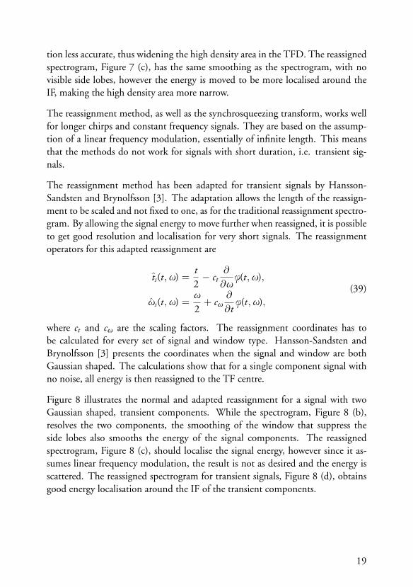
tion less accurate, thus widening the high density area in the TFD. The reassignedspectrogram, Figure 7 (c), has the same smoothing as the spectrogram, with novisible side lobes, however the energy is moved to be more localised around theIF, making the high density area more narrow.

The reassignment method, as well as the synchrosqueezing transform, works wellfor longer chirps and constant frequency signals. They are based on the assump-tion of a linear frequency modulation, essentially of infinite length. This meansthat the methods do not work for signals with short duration, i.e. transient sig-nals.

The reassignment method has been adapted for transient signals by Hansson-Sandsten and Brynolfsson [3]. The adaptation allows the length of the reassign-ment to be scaled and not fixed to one, as for the traditional reassignment spectro-gram. By allowing the signal energy to move further when reassigned, it is possibleto get good resolution and localisation for very short signals. The reassignmentoperators for this adapted reassignment are

ts(t,ω) =t2− ct

∂

∂ωφ(t,ω),

ωs(t,ω) =ω

2+ cω

∂

∂tφ(t,ω),

(39)

where ct and cω are the scaling factors. The reassignment coordinates has tobe calculated for every set of signal and window type. Hansson-Sandsten andBrynolfsson [3] presents the coordinates when the signal and window are bothGaussian shaped. The calculations show that for a single component signal withno noise, all energy is then reassigned to the TF centre.

Figure 8 illustrates the normal and adapted reassignment for a signal with twoGaussian shaped, transient components. While the spectrogram, Figure 8 (b),resolves the two components, the smoothing of the window that suppress theside lobes also smooths the energy of the signal components. The reassignedspectrogram, Figure 8 (c), should localise the signal energy, however since it as-sumes linear frequency modulation, the result is not as desired and the energy isscattered. The reassigned spectrogram for transient signals, Figure 8 (d), obtainsgood energy localisation around the IF of the transient components.

19

Figure 8: Illustration of reassignment for a transient signal; (a) time representa-tion; (b) spectrogram; (c) reassigned spectrogram; (d) reassigned spectrogram fortransient signals.

In order to achieve faster computations of the reassignment coordinates a differentformulation can be used

tx(t,ω) = t + ctR

(F th

x (t,ω)F h

x (t,ω)

),

ωx(t,ω) = ω− cωI

(F dh/dt

x (t,ω)F h

x (t,ω)

),

(40)

20

where R and I represents the real and imaginary parts and F hx , F th

x and F dh/dtx are

the STFTs with different time windows. The formulation, without the scalingfactors, is presented in [25].

An other adaptation of the reassigned spectrogram was presented by Auger et al.[28], it uses the Levenberg-Marquardt algorithm [29, 30], to allow for a weak orstrong reassignment. The reassignments coordinates are derived from the second-order partial derivatives of the phase of the STFT, and it is possible to get goodlocalisation of long or short signal by adjusting a dampening parameter. Themethod requires the additional calculation of one more STFT with the time win-dow t2h(t). A recursive implementation of the Levenberg-Marquardt reassign-ment has also been proposed recently [1].

21

5 Main results of the research papers

All three papers in this thesis concern the TF analysis of non-stationary and multi-component signals. The aim of the papers involve finding high resolution TF rep-resentations of different signals. Paper A and B have more practical applicationsand paper C is more theoretical. This section outlines the papers.

Paper A: Optimal time–frequency distributions using a novel signaladaptive method for automatic component detection

Paper A presents a signal adaptive method for automatically detecting signal com-ponents in two-component signals. The method is based on, and outperforms, amethod presented by Sucic and Boashash [31]. In the paper the new method isused with a quantitative performance measure presented by Boashash and Sucic[22] with the aim of finding the optimal, high resolution TFD for long duration,frequency modulated (FM) signals with two close components.

The proposed method is shown to accurately detect signal components for dif-ferent types of two component FM signals. The evaluation is done on simulatedsignals with white Gaussian noise, and the method is found to be insensitive toamplitude differences of the components, frequency distance between the com-ponents and smoothing of the TFD. Since the method is robust to the level ofsmoothing of the TFD, a large range of TFDs can be tested, lowering the risk oferroneous conclusions to be drawn of the optimal TFD.

To illustrate the use of the method, with the performance measure, the papershows how the optimal kernel parameters for the modified B-distribution [32] ofan example set of heart rate variability (HRV) signals with a non-linear compon-ent can be obtained. HRV, which is the variation of inter-heartbeat intervals, ismeasured non-invasively using ECG and is a sensitive indicator of compromisedhealth [7, 33]

22

Paper B: Objective detection and time-frequency localization of com-ponents within transient signals

Paper B presents a method that automatically detects and counts transient signalcomponents in a signal with an unknown number of components. The paperalso thoroughly investigates the reassigned spectrogram for transient signals [3],which is used in the detection method. The TFD is found to have good TFresolution even for noisy signals, i.e. it resolves heavily overlapping components.The method is unique in that it is developed for short transient signals, othercomponent detection methods are designed for longer signals.

The aim of the automatic detection method is to give the TF centres of allcomponents within a multi-component, transient signal. The evaluation of themethod shows that the estimated TF centres have good accuracy and that the cor-rect number of components almost always are detected for a variety of transientsignals with white Gaussian noise. For the evaluation, the transient componentsare Gaussian shaped, which is an usual assumption for transients.

Promising results are shown when the method is tested on measured data froma laboratory pulse-echo set-up and from a dolphin echolocation signal measuredsimultaneously at two different locations in the echolocation beam. This is ofgreat interest since transient signals are common in several fields, e.g. ultrasonicand marine biosonar signal analysis, machine fault diagnosis and biomedical sig-nal processing [8, 9, 34, 35, 36].

Paper C: The scaled reassigned spectrogram adapted for detection andlocalisation of transient signals

Paper C builds on the reassigned spectrogram for transient signals [3] and presentsthe reassignment coordinates for when the signal and time window of the spec-trogram are combinations of the first and second Hermite functions. The aim ofthe paper is to show that it is possible to get perfect localisation, i.e. that all signalenergy is reassigned to the TF centre of the signal, not only for signals that areGaussian shaped.

It has previously been shown that for a transient, Gaussian (first Hermite func-tion) shaped signal it is possible to get perfect localisation after reassignment ifa Gaussian shaped window is used for the spectrogram [3]. This paper shows

23

that perfect localisation is also possible for a signal with the shape of the secondHermite function, if the time window used for the spectrogram is also a secondHermite function. It is also shown that perfect localisation is not possible toachieve if matching a Gaussian signal with a second Hermite window, or a secondHermite signal with a Gaussian window, then instead the signal energy is scatteredin ellipses. The Hermite functions are analysed since they can be combined lin-early to model transient signals [37, 38, 39, 40].

Perfect localisation is only possible for single component signals without noise,however the signal energy for multi-component signals with noise is still local-ised after reassignment if the signal and window shapes match. When the signaland window shapes do not match, the signal energy will appear more scattered.This can be used to detect the shape of and localise the TF centres of individualtransient components in a non-stationary signal.

The results from simulated multi-component signals with white Gaussian noiseshow that close components can be resolved and correctly identified as beingeither Gaussian or second Hermite shaped. Good results are obtained even forsignals heavily disturbed by noise. For a measured dolphin echolocation signal, itappears that two Gaussian-like components can be detected.

24

References

[1] D. Fourer, F. Auger, and P. Flandrin, “Recursive versions of the Levenberg-Marquardt reassigned spectrogram and of the synchrosqueezed STFT,” in2016 IEEE International Conference on Acoustics, Speech and Signal Processing(ICASSP), March 2016, pp. 4880–4884.

[2] N. Saulig, I. Orovic, and V. Sucic, “Optimization of quadratic time-frequency distributions using the local Renyi entropy information,” SignalProcessing, vol. 129, pp. 17–24, 2016.

[3] M. Hansson-Sandsten and J. Brynolfsson, “The scaled reassigned spectro-gram with perfect localization for estimation of Gaussian functions,” IEEESignal Processing Letters, vol. 22, no. 1, pp. 100–104, January 2015.

[4] L. Stankovic, I. Djurovic, S. Stankovic, M. Simeunovic, S. Djukanovic,and M. Dakovic, “Instantaneous frequency in time-frequency analysis: En-hanced concepts and performance of estimation algorithms,” Digital SignalProcessing, vol. 35, pp. 1–13, December 2014.

[5] F. Auger, P. Flandrin, Y.-T. Lin, S. McLaughlin, S. Meignen, T. Oberlin, andH.-T. Wu, “Time-frequency reassignment and synchrosqueezing,” IEEESignal Processing Magazine, pp. 32–41, November 2013.

[6] V. Maganin, T. Bassani, V. Bari, M. Turiel, R. Maestri, G. D. Pinna, and A.Porta, “Non-stationarities significantly distort short-term spectral, symbolicand entropy heart rate variability indices,” Physiological Measurement, vol.32, pp. 1775–1786, 2011.

[7] M. T. Verklan and N. S. Padhye, “Spectral analysis of heart rate variabil-ity: An emerging tool for assessing stability during transition to extrauterine

25

life,” Journal of Obstetric, Gynecologic & Neonatal Nursing, vol. 33, no. 2,pp. 256–265, 2004.

[8] J. Pons-Llinares, M. Riera-Guasp, J. A. Antonino-Daviu, and T. G. Ha-betler, “Pursuing optimal electric machines transient diagnosis: The adapt-ive slope transform.,” Mechanical Systems and Signal Processing, vol. 80, pp.553 – 569, 2016.

[9] Q. He and X. Ding, “Sparse representation based on local time-frequencytemplate matching for bearing transient fault feature extraction.,” Journal ofSound and Vibration, vol. 370, pp. 424 – 443, 2016.

[10] W.W.L. Au, B. Branstetter, P.W. Moore, and J.J. Finneran, “Dolphin bio-sonar signals measured at extreme off-axis angles: Insights to sound propaga-tion in the head,” J. Acoust. Soc. Am., vol. 132, no. 2, pp. 1199–1206, 2012.

[11] T. W. Cranford, W. R. Elsberry, W. G. Van Bonn, J. A. Jeffress, M. S.Chaplin, D. J. Blackwood, D. A. Carder, T. Kamolnick, M. A. Todd, andS. H. Ridgway, “Observation and analysis of sonar signal generation in thebottlenose dolphin (tursiops truncatus): Evidence for two sonar sources,”Journal of Experimental Marine Biology and Ecology, vol. 407, no. 1, pp. 81– 96, 2011.

[12] J. Starkhammar, P.W.B. Moore, L. Talmadge, and D.S. Houser, “Frequency-dependent variation in the two-dimensional beam pattern of an echolocat-ing dolphin,” Biol. Lett., vol. 7, no. 6, pp. 836–839, 2011.

[13] L. Cohen, Time-Frequency Analysis, Signal Processing Series. Prentice-Hall,Upper Saddle River, NJ, USA, 1995.

[14] D. Gabor, “Theory of communications,” Journal of the IEE, vol. 93, pp.429 – 460, 1946.

[15] B. Boashash, “Part I: Introduction to the concepts of TFSAP,” in Time Fre-quency Signal Analysis and Processing - A Comprehensive Reference, BoualemBoashash, Ed. Elsevier Ltd, Oxford, 1994.

[16] H.-I. Choi and W. J. Williams, “Improved time-frequency representation ofmulti-component signals using exponential kernels,” IEEE Trans. Acoustics,Speech and Signal Processing, vol. 37, pp. 862–871, June 1989.

26

[17] R. Liao, C. Guo, Ke Wang, Z. Zuo, and A. Zhuang, “Adaptive optimal ker-nel time-frequency representation technique for partial discharge ultra-high-frequency signals classification,” Electric Power Components and Systems, vol.43, no. 4, pp. 449–460, 2015.

[18] R. G. Baraniuk and D. L. Jones, “A signal-dependent time-frequency rep-resentation: Optimal kernel design,” IEEE Transactions on Signal Processing,vol. 41, no. 4, pp. 1589 – 1602, 1993.

[19] M. J. Bastiaans, “Gabor’s expansion of a signal into Gaussian elementarysignals,” Proc. of the IEEE, vol. 68, no. 4, pp. 538–539, April 1980.

[20] S.C. Pei and S.G. Huang, “STFT with adaptive window width based on thechirp rate,” IEEE Transactions on Signal Processing, vol. 60, no. 8, pp. 4065– 4080, 2012.

[21] R. G. Baraniuk, P. Flandrin, A. J. E. M. Janssen, and O. J. J. Michel, “Meas-uring time-frequency information content using Renyi entropies,” IEEETrans. on Information Theory, vol. 47, no. 4, pp. 1391–1409, May 2001.

[22] B. Boashash and V. Sucic, “Resolution measure criteria for the objectiveassessment of the performance of quadratic time-frequency distributions,”Signal Processing, vol. 51, pp. 1253–1263, 2003.

[23] M. Abed, A. Belouchrani, and B. Boashash, “Time-frequency distributionsbased on compact support kernels: Properties and performance evaluation,”Signal Processing, vol. 60, no. 6, pp. 2814–2827, June 2012.

[24] K. Kodera, C. de Villedary, and R. Gendrin, “A new method for the nu-merical analysis of nonstationary signals,” Physics of the Earth & PlanetaryInteriors, vol. 12, pp. 142–150, 1976.

[25] F. Auger and P. Flandrin, “Improving the readability of time-frequency andtime-scale representations by the reassignment method,” IEEE Trans. onSignal Processing, vol. 43, pp. 1068–1089, May 1995.

[26] I. Daubechies, J. Lu, and H.-T. Wu, “Synchrosqueezed wavelet transforms:An empirical mode decomposition-like tool.,” Applied & ComputationalHarmonic Analysis, vol. 30, no. 2, pp. 243 – 261, 2011.

27

[27] N. E. Huang and Z. Wu, “A review on Hilbert-Huang transform: Methodand its applications to geophysical studies,” Reviews of Geophysics, vol. 46,no. 2, pp. n/a–n/a, 2008, RG2006.

[28] F. Auger, E. Chassande-Mottin, and P. Flandrin, “Making reassignment ad-justable: The Levenberg-Marquardt approach,” in 2012 IEEE InternationalConference on Acoustics, Speech and Signal Processing (ICASSP), March 2012,pp. 3889–3892.

[29] K. Levenberg, “A method for the solution of certain non-linear problems inleast squares,” Quarterly of Applied Mathematics, vol. 2, no. 2, pp. 164-168,1944.

[30] D. Marquardt, “An algorithm for least-squares estimation of nonlinear para-meters,” SIAM Journal on Applied Mathematics, vol. 11, no. 2, pp. 431-441,1963.

[31] V. Sucic and B. Boashash, “Parameter selection for optimising time-frequency distributions and measurements of time-frequency characteristicsof non-stationary signals,” in IEEE International Conference on Acoustics,Speech, and Signal Processing, 2001, vol. 6, pp. 3557–3560.

[32] Z. M. Hussain and B. Boashash, “Multi-component IF estimation,” inStatistical Signal and Array Processing, August 2000, pp. 559 – 563.

[33] G. G. Berntson, J. T. Bigger, JR., D. L. Eckberg, P. Grossman, P. G.Kaufmann, M. Malik, H. N. Nagaraja, S. W. Porges, J. P. Saul, P. H. Stone,and M. W. Van Der Molen, “Heart rate variability: Origins, methods, andinterpretive caveats,” Psychophysiology, vol. 34, pp. 623–648.

[34] C. Wei, W. W. L. Au, D. R. Ketten, Z. Song, and Y. Zhang, “Biosonarsignal propagation in the harbor porpoise’s (Phocoena phocoena) head: Therole of various structures in the formation of the vertical beam.,” Journal ofthe Acoustical Society of America, vol. 141, no. 6, pp. 4179, 2017.

[35] H. Liu, Weiguo Huang, S. Wang, and Z. Zhu, “Adaptive spectral kurtosisfiltering based on morlet wavelet and its application for signal transientsdetection.,” Signal Processing, vol. 96, no. Part A, pp. 118 – 124, 2014.

28

[36] C. Capus, Y. Pailhas, K. Brown, D.M. Lane, P. Moore, and D. Houser,“Bio-inspired wideband sonar signals based on observations of the bottlen-ose dolphin (Tursiops truncatus),” J. Acoust. Soc. Am., vol. 121, no. 1, pp.594–604, 2007.

[37] R. Ma, Z. Huang L. Shi, and Y. Zhou, “EMP signal reconstruction usingassociated-Hermite orthogonal functions,” IEEE Trans. on ElectromagneticCompatibility, vol. 64, no. 6, pp. 1383–1390, March 2016.

[38] B.N. Li, M.C. Dong, and M.I. Vai, “Modeling cardiovascular physiologicalsignals using adaptive Hermite and wavelet basis functions,” IET SignalProcessing, vol. 4, no. 5, pp. 588–597, 2010.

[39] T. H. Linh, S. Osowski, and M. Stodolski, “On-line heart beat recogni-tion using Hermite polynomials and neuro-fuzzy network,” IEEE Trans. onInstrumentation and Measurement, vol. 52, no. 4, pp. 1224–1231, August2003.

[40] A.I. Rasiah, R. Togneri, and Y. Attikiouzel, “Modeling 1-D signals usingHermite basis functions,” in IEEE Proc.-Vis. Image Signal Process. IEEE,1997, vol. 144, pp. 345–354.

29

Scientific publications

Author contributions

Co-authors are abbreviated as follows:Maria Sandsten (MS), Josefin Starkhammar (JS).

Paper A: Optimal time–frequency distributions using a novel signaladaptive method for automatic component detection

I had the idea for the paper and developed the presented algorithm, however withinvaluable guidance from MS. I did the simulations and had the main responsib-ility for the writing.

Paper B: Objective detection and time-frequency localization of com-ponents within transient signals

MS, JS and I came up with the idea for the paper. I developed the presenteddetection algorithm, with valuable support from MS. I did the testing on thesimulated data, while JS did the testing on the dolphin echolocation data. JS alsocollected and worked with the ultra sound pulse-echo data. Everyone collaboratedwith the writing, MS had the main responsibility for the introduction, includingfinding related research, JS had the main responsibility for the examples section,and I for the rest.

31

Paper C: The scaled reassigned spectrogram adapted for detection andlocalisation of transient signals

MS and I developed the idea for the paper. I did the calculations presented andsimulations, with support from MS. The data for the dolphin echolocation ex-ample was recorded by JS, who also contributed to the text in the example section.MS provided information on previous research and I had main responsibility forthe writing.

32

Paper A

Paper A

Optimal time–frequency distributionsusing a novel signal adaptive method forautomatic component detection

Isabella Reinhold, Maria Sandsten

Mathematical Statistics, Centre for Mathematical Sciences, Lund University,Sweden.

Abstract

Finding objective methods for assessing the performance of time-frequencydistributions (TFD) of measured multi-component signals is not trivial.An optimal TFD should have well resolved signal components (auto-terms) and well suppressed cross-terms. This paper presents a novel signaladaptive method, which is shown to have better performance than the ex-isting method, of automatically detecting the signal components for TFDtime instants of two-component signals. The method can be used togetherwith a performance measure to receive automatic and objective perform-ance measures for different TFDs, which allows for an optimal TFD to beobtained. The new method is especially useful for signals including auto-terms of unequal amplitudes and non-linear frequency modulation. Themethod is evaluated and compared to the existing method, for finding theoptimal parameters of the modified B-distribution. The performance isalso shown for an example set of Heart Rate Variability (HRV) signals.

Keywords: time-frequency, multi-component signal, detection,performance measure, Heart Rate Variability

35

1 Introduction

There are many types of non-stationary signals, most of which are multi-component. These signals need to be visualised in time and frequencysimultaneously to characterise their time-varying nature. To do this thedistribution of the signal energy over the time-frequency plane, i.e. thetime-frequency distribution (TFD), can be studied.

The Wigner-Ville distribution (WVD) is a common TFD. For mono-component, linear frequency modulated (FM) signals the WVD gives ex-actly the instantaneous frequency (IF) making it the optimal TFD for suchsignals. The problem with the WVD occurs when dealing with multi-component signals or signals disturbed by noise. For such a signal theWVD is not always zero when the signal has no power for a given time-frequency instant. These contributions are called cross-terms and can havetwice the amplitude of the signal components. This makes it difficult todistinguish the actual signal components, also called auto-terms, from thecross-terms, [1].

There exist many TFDs which aim to suppress cross-terms by means of fil-tering the WVD with a kernel, such as Choi-Williams, Zhao-Atlas-Marks[1] and modified B-distribution [2]. However suppression of the cross-terms can also result in loss of resolution of the signal components. Find-ing good representations of multi-component signals is a complex problemand is still a large field of research [3, 4]. When looking at different TFDsfor multi-component signals it might be possible to say that some plotslook cleaner and thus better. However, assessing the performance basedonly on this visual comparison is very subjective and finding the optimalparameter for a specific kernel would be very tiresome if not impossible.Not many methods exist, for assessing which TFD is the best for a givensignal, especially when dealing with measured signals.

A quantitative performance measure for TFDs of two-component signals,called normalised instantaneous resolution (NIR) performance measure,was presented in [5]. The NIR performance measure makes it possibleto compare different TFDs and optimise kernel parameters which controlthe tradeoff between signal component resolution and cross-term suppres-

36

sion. The NIR performance measure can be used for simulated as well asmeasured signals and was recently used in [6, 7] to find optimal TFDs fordifferent multi-component signals. However, the measure relies on para-meters connected to correct detection of the signal components for eachtime instant of the TFD, and the method used for automatic detection ofauto-terms is the one presented in [8]. One restriction of this method is therequirement that the amplitudes of the two signal components are (approx-imately) equal, which is an assumption that limits the use of the method.The method also fails when signal components are close to each other orhas components with non-linear FM law [9], which is a well known re-striction of many methods [3]. These restrictions in the detection methodnarrows the use of the NIR performance measure as the choice of analysedkernel parameters needs to be made with care. This limits the use of theperformance measure for automatic optimisation of signal adaptive ker-nels, compared to other methods such as [10]. A large number of methodsfor identification of signal components exist, e.g. [11, 12, 13], who re-quire that cross-terms are well suppressed and locates the maximum peaksas signal components. Other methods such as [14] which uses a methodcalled non-linear squeezing time-frequency transform exist as well. How-ever, these methods require already optimised or semi-optimised TFDs orare more complex and computationally heavy.

This paper presents a new signal adaptive method for automatically de-tecting signal components in two-component signals which outperformsthe method in [8]. The new method is not limited by requiring that thesignal components have equal amplitudes. Additionally, the method suc-ceeds in detecting components with non-linear FM laws. Further, thenew algorithm overcomes one of the main drawbacks when the estimatedparameters are used in the NIR performance measure, as it successfullyidentifies auto-terms for a larger interval of kernel parameters, allowingfor a more objective kernel optimisation. It is also feasible that for two-component signals the new automatic detection method can be used tofind the direction of the auto-terms which is used to create an adaptivedirectional kernel [15, 16]. This kernel smooths at each point in the time-frequency domain based on the direction of the energy distribution of thesignal.

37

To illustrate the use of the new signal adaptive automatic detection methodtogether with the NIR performance measure, this paper shows how the op-timal kernel parameters for the modified B-distribution [2] of an exampleset of Heart Rate Variability (HRV) signals with a non-linear componentcan be obtained. HRV, which is the variation of inter-heartbeat intervals, ismeasured non-invasively using ECG. It provides information on the auto-nomic regulation of the cardiovascular system. This means that the HRVis a sensitive indicator of compromised health [17, 18]. The HRV has anon-stationary nature, however only recently methods which do not as-sume stationarity have been evaluated for HRV [19, 20]. It is commonto study HRV during treadmill running [21, 22], making the need formethods of studying HRV in time and frequency concurrently even moreimportant.

The paper is organised as follows. Section 2 provides an introduction tothe basics of time-frequency analysis. Section 3 shortly presents the NIRperformance measure which will be used and details the new signal adapt-ive method for automatic detection of the signal components. In Section4 the performance of the new automatic detection method is evaluatedand compared to the performance of the method in [8]. The basis for theevaluation is simulated signals and an example set of HRV signals. Theoptimal modified B-distributions of the example HRV signals are presen-ted in Section 5. Sections 6 and 7 finish the paper with discussion andconclusions.

2 Time-frequency methods

The Wigner-Ville distribution (WVD),

Wz(t, f ) =∫ ∞−∞

z(t + τ

2

)z∗(t − τ

2

)e−i2πf τdτ, (1)

where ∗ represents the complex conjugate, is a TFD defined using an ana-lytic signal, z(t). The analytic signal is defined such that Z (f ) = 0 iff < 0, where Z (f ) = F{z(t)}, is the Fourier transform of the signal. Thequadratic class of TFDs, a subclass of TFDs where the signal kernel is of

38

quadratic form, can be written as

ρz(t, f ) =∫ ∞−∞

∫ ∞−∞

G(t − u, τ)z(u + τ

2

)z∗(u− τ

2

)e−i2πf τdudτ, (2)

where the time-lag kernel G(t, τ) is specific for each different quadraticTFD. The convolution of the kernel in (2) is (in most cases) equal to a2D filtering of the TFD and is used to suppress cross-terms. The design ofthe kernels is usually done in the ambiguity (doppler-lag) domain, whereauto- and cross-terms are more easily differentiable [1].

2.1 Separable and lag-independent kernels

One simple, yet useful, class of kernels is the separable kernels. With theseparable kernel the TFD can be written

ρz(t, f ) = g1(t) ∗t

Wz(t, f ) ∗f

G2(f ). (3)

The convolutions in time and frequency can now be made in either orderwhich simplifies the calculations. It also means that the design of the kernelwill be greatly simplified, the 2D filtering operation is replaced by twoconsecutive 1D filtering operations. A special case of the separable kernelis the lag-independent (LID) kernel. It is obtained by setting

G2(f ) = δ(f ), (4)

which means that the kernel only will depend on time t. The calculationsfor the TFD then only require one convolution, in the time direction only

ρz(t, f ) = g1(t) ∗t

Wz(t, f ). (5)

Since the LID kernel only applies one 1D filtering, the resulting TFD willbe smoothed in the time direction only. This property makes the LIDkernel suitable for slowly varying frequency modulated signals or othersignals where cross-terms exist mainly some frequency distance from theauto-terms and single auto-terms do not vary much in frequency. LID-TFDs have been shown to have better performance in characterising HRV

39

signals, compared to other time-frequency methods [23]. The LID ker-nel can have different distributions, one is the modified B-distribution(MBD), which has been shown to be suitable for HRV signals [24]. TheMBD kernel is defined as

gMBD(t) =cosh−2β (t)∫∞

−∞ cosh−2β (ξ)dξ, (6)

where β is the scaling parameter which determines the trade-off betweenresolution of signal components and cross-term suppression. The MBD,designed specifically for multi-component IF estimation, is almost cross-term free and has high resolution of signal components in the time-frequency plane [2].

3 Performance measure and a novel signal adaptivemethod for automatic detection of auto-terms

The NIR performance measure, which combines the concepts of high en-ergy concentration around the IF laws and clearly resolved signal com-ponents is presented in [5]. The measure doesn’t take into account someproperties usually demanded for TFDs, which impose strict constraints onthe TFD design, such as satisfying the marginals [1]. Instead it focuseson resolution of signal components and suppression of cross-terms andsidelobes, which are important for practical use. The measure is defined as

P(t) = 1− 13

(AS(t)AM (t)

+12

AX (t)AM (t)

+ (1− D(t))), 0 ≤ P(t) ≤ 1, (7)

where AS(t) is the average absolute amplitude of the largest sidelobes,AM (t) the average amplitude of the auto-terms (mainlobes), AX (t) the ab-solute amplitude of the cross-term and D(t) a measure of the separation ofthe signal components’ mainlobes. It is defined as

D(t) =

(f2(t)− V2(t)

2

)−(f1(t)− V1(t)

2

)f2(t)− f1(t)

, (8)

40

where f1(t) and f2(t) are the centres of the mainlobes and V1(t) and V2(t)are the instantaneous bandwidths of the auto-terms, calculated at

√2/2 of

the height of the mainlobe.

For this measure a value close to 1 is a good performance. The perform-ance measure is calculated for a time instant (slice) of the TFD. If P(t) iscalculated for several time instants, an estimate of the performance for thewhole TFD can be formed [5]. This measure works well for signals withboth linear and non-linear FM components [8, 9]. The only restriction isthat the signal should have only two components where the performancemeasure is calculated.

3.1 A novel signal adaptive method for automatic detection of auto-terms

In order to use the resolution performance measure on signals there isa need for a signal adaptive method which automatically detects auto-,cross-terms and sidelobes for a TFD time slice. Such a method for two-component signals is proposed by Sucic et al. [8]. However, the difficultylies within detecting the auto-terms and a restriction is the assumption thatthe signal components have equal amplitudes. The algorithm for Sucic’sautomatic detection of auto-terms (ADAT) follows these steps:

1. Normalise the time slice such that the absolute maximum is equal to1.

2. Determine the three largest maxima (peaks) of the slice.

3. The cross-term is located between the auto-terms, so initially set themiddle peak to be the cross-term and the remaining as auto-terms.

4. Make sure that the ratio between the amplitudes of remaining twopeaks is close to 1, and that the peak chosen as the cross-terms is closeto the middle point between the centres of the other two peaks. Thischecks whether the assumption in the previous step is correct. If not,select the two largest peaks of the slice as the auto-terms.

41

This method is simple and does in many cases successfully identify theauto-terms. However, the requirement that the amplitudes of the twosignal components are (approximately) equal limits its use. Another draw-back is that the method has a degraded performance for signals contain-ing components with non-linear frequency modulated (FM) law [9]. Thenovel method presented here does not require the signal component amp-litudes to be equal, instead it relies on sidelobes and noise peaks of re-stricted amplitudes. The steps of the novel Reinhold’s ADAT algorithmare:

1. Normalise the time slice such that the absolute maximum is equal to1.

2. Determine an amplitude threshold, λ, for the auto-terms.

3. Determine between which frequencies all peaks above λ are located.This is the estimated frequency distance between the auto-terms,Δfa. Set δ ≈ Δfa/2 as the minimum allowed frequency distancebetween the auto- and cross-terms.

4. Identify the largest peaks above the threshold λ, which are separatedwith at least δ. These are the only peaks which will be consideredwhen identifying auto-terms. Select the peaks furthest away fromeach other as the auto-terms.

The minimum distance δ is set as approximately half the estimated fre-quency distance between the auto-terms since theoretically within Δfathere should be three peaks, the two auto-terms and the cross-term. It isreasonable to choose it as δ = Δfa/2−ε, where ε is a small error tolerance.This allows for some error in the estimation ofΔfa and small deviations ofthe placement of the cross-term.

The selection of the parameter λ could also be made automatically andshould be allowed to vary with each time slice for optimal results. Thispaper proposes to let λ = cA2, where A2 is the amplitude of the secondlargest peak and c is some scale factor, 0 < c < 1. This means that λalways will relate to the amplitudes of the signal content. For simulations

42

Figure 1: Time slice of the WVD of a two-component linear FM signal, withIFs 0.15 and 0.22; (a) Potential auto-terms detected with Sucic’s ADAT, markedwith circles; (b) Detected auto-terms with Reinhold’s ADAT, the auto-terms aremarked by circles and the labels f1 and f2 respectively. The horizontal line showsthe threshold λ and the dashed lines are δ away from each identified auto-term.

in this paper λ = 0.5A2, if nothing else is stated. Other choices of c canbe used and Section 4.1 will evaluate how robust the novel ADAT is todifferent λs.

3.2 Motivation for new automatic detection method

This section will motivate the need for a new ADAT by studying twoexample time slices from TFDs of two-component signals. The examplesdemonstrate situations when Sucic’s ADAT fails to correctly detect theauto-terms, whereas Reinhold’s ADAT is successful. The first example isa time slice of a WVD of a signal with components of equal amplitude.Sucic’s ADAT initially identifies the three largest peaks, if these peaks areclose in amplitude, two of them are identified as auto-terms. Figure 1(a)shows the identified three peaks. The ratio between any two of these peaksis close to one and thus two of the three peaks are identified as auto-terms,which two depend on implementation choices for the algorithm. Howeversince the first auto-term is not among these peaks Sucic’s ADAT fails tocorrectly identify the auto-terms.

43

Figure 2: Time slice of a LID-TFD of a two-component non-linear FM signal,with IFs 0.15 and 0.19; (a) Auto-terms detected by Sucic’s ADAT, marked bycircles; (b) Auto-terms detected by Reinhold’s ADAT, marked by circles and thelabels f1 and f2 respectively. The horizontal line shows the threshold λ and thedashed lines are δ away from each identified auto-term.

In this example only four peaks are above the threshold λ, marked by ahorizontal line in Figure 1(b). The peaks of maximum distance are initiallyidentified as the auto-terms, which gives an estimate of Δfa. Reinhold’sADAT will then detect three peaks above λ which are separated by at leastδ, the auto-terms and one of the dual peaks of the cross-term. The distancebetween the dual peaks of the cross-term is (much) smaller than δ, henceonly one of the peaks are detected. Of the three detected peaks, the two atmaximum distance are finally identified as the auto-terms. These two arethe actual auto-terms and they are marked in the figure by the labels f1 andf2. The figure also shows, in dashed lines, f1 ± δ and f2 ± δ.

The second example is a time slice from a LID-TFD of a signal with non-linear FM law for one component, where the signal components haveequal amplitude. However, for some time slices of the TFD, there willbe poor energy concentration around the non-linear component’s IF law,which will result in differences in the amplitudes of the auto-terms. Ac-cording to Sucic’s ADAT, after identification of the three largest peaks, ifthe ratio between the two outer peaks is not close to one, the two largestpeaks are chosen as auto-terms. Figure 2(a) shows how these steps identi-fies the wrong peaks as auto-terms.

44

Reinhold’s ADAT correctly identifies the auto-terms of this time slice,which is shown in Figure 2(b). As seen in the figure, only three peaksare above the threshold λ, the outermost are the auto-terms and those areidentified as auto-terms. Figure 2(b) also shows f1 ± δ and f2 ± δ.

3.3 Signals with more than two components

The purpose of the NIR performance measure is to resolve two compon-ents which are close in frequency, however it can still be interesting to re-solve close components in a signal with more than two components. Thereare two kinds of signals which are particularly interesting to consider, bothhas three components, however one has only two components present inthe signal at any given time. For such a signal there is no theoretical prob-lem using the ADAT algorithms, since the signal’s TFD is analysed at eachtime instant. Therefore it does not matter how long time duration signalcomponents have or how many signal components the signal has, as longas there are at maximum two for any given time instant.

An example of the other type of three component signal is defined by

s(n) = cos(2π(0.15 + 0.04

(n

256

))n)+ cos

(2π(0.24− 0.04

(n

256

))n)

+ cos(2π0.3n), 0 < n ≤ 256,(9)

and shown in Figure 3, it has three components which are all present at thesame time. This signal presents a problem for both ADAT methods, sincethey are designed to find only two auto-terms separated by some frequencydistance in each time instant, and both methods usually fail to identify thedesired auto-terms for such a signal.

However the NIR performance measure and ADAT algorithms can still beused for such signals if only the possibly known frequency band containingthe two close components are considered. The ADAT methods will thenonly be applied to that frequency band and this requires omitting parts ofthe TFD beforehand. In this example the NIR performance is calculatedin the frequency band 0 - 0.25. Figures 4(a) and (b) shows the detected

45

Figure 3: MBD of the signal (9), which is a three component signal with twoclose components and one further away.

Figure 4: Detection of auto-terms in the example three-component signal (9),when only considering the frequency band 0 - 0.25 in the ADAT algorithms; (a)Sucic’s ADAT; (b) Reinhold’s ADAT.

auto-terms on top of the TFDs for Sucic’s and Reinhold’s ADAT respect-ively. The methods perform similarly and identifies the correct auto-termsfor most time instants. The added disturbance of more cross-terms candecrease the performance of both ADAT algorithms and some initial fil-tering with an appropriate kernel might be needed to suppress cross-terms.An indication that filtering by a kernel is needed is if the auto-terms arehard to distinguish by eye. The suggestion is then to apply a wide kernelto get a TFD which closely resembles the WVD, keeping the resolution ofthe auto-terms, but with cross-terms slightly suppressed. In this examplea wide MBD-kernel (β = 0.5) is used, the performance of both meth-

46

ods increase if the kernel is more narrow. If the kernel is instead mademore wide, the middle auto-term will be very hard to distinguish from thecross-term which intercepts it.

4 Detection of auto-terms

To compare the performance of Sucic’s and Reinhold’s ADAT, the rate ofdetection for different two-component signals and TFDs have been stud-ied. The rate of detection is measured by checking if the detected auto-terms are close to the signal component IFs in each time slice of the TFD.The detection for each time instant can be either successful or unsuccess-ful. If the frequencies of both the detected auto-terms vary no more thanΔfa/4 from the respective signal component IF, the detection is called suc-cessful. Every successful detection yields a value 1 and every unsuccessfula 0. The detection results for each time instant of the TFD is then addedtogether and the sum is divided by the number of time instants, this givesa rate of detection in the interval [0, 1] for the whole signal.

In this section the rate of detection will be examined for signals with addit-ive Gaussian white noise, with signal-to-noise ratio (SNR) 5 dB. The rateof detection for a given signal will vary with different noise simulations.Thus to give an accurate description of the rate of detection, 500 differ-ent noise simulations will be used to find the average rate of detection fora given signal and kernel parameter. The lower bound of the one sidedconfidence interval with 5% significance is also presented.

When computing the TFD of a (finite) signal, there will be some effectsaround the edges, in time and frequency. In this section, the middle 2/3time slices of the TFD will be evaluated when calculating the rate of de-tection, where the initial and end time slices are ignored. The simulatedsignals are 256 samples, which gives 256 · 2/3 = 172 evaluated time in-stants for each TFD.

47

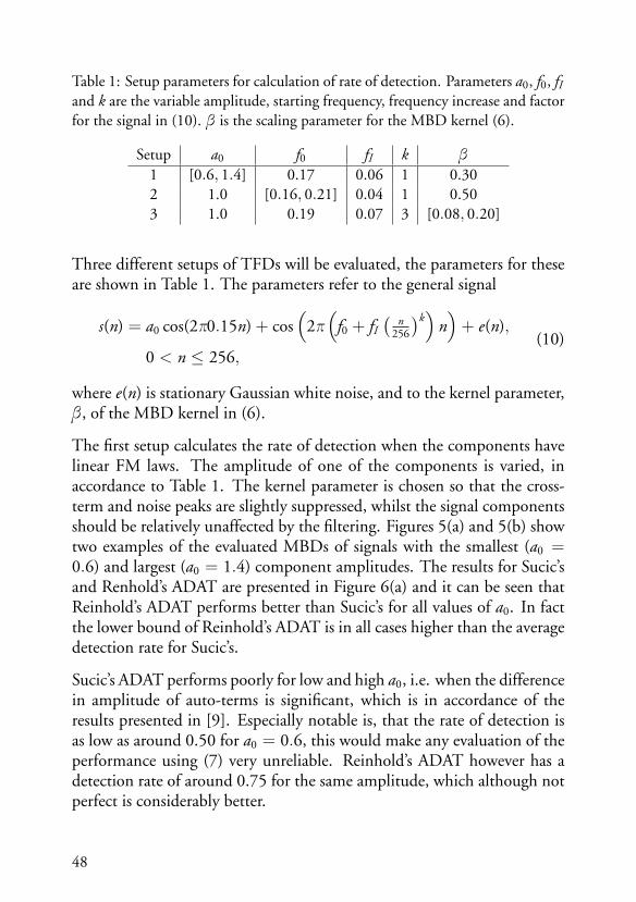
Table 1: Setup parameters for calculation of rate of detection. Parameters a0, f0, fIand k are the variable amplitude, starting frequency, frequency increase and factorfor the signal in (10). β is the scaling parameter for the MBD kernel (6).

Setup a0 f0 fI k β

1 [0.6, 1.4] 0.17 0.06 1 0.302 1.0 [0.16, 0.21] 0.04 1 0.503 1.0 0.19 0.07 3 [0.08, 0.20]

Three different setups of TFDs will be evaluated, the parameters for theseare shown in Table 1. The parameters refer to the general signal

s(n) = a0 cos(2π0.15n) + cos(

2π(

f0 + fI(

n256

)k)

n)+ e(n),

0 < n ≤ 256,(10)

where e(n) is stationary Gaussian white noise, and to the kernel parameter,β , of the MBD kernel in (6).

The first setup calculates the rate of detection when the components havelinear FM laws. The amplitude of one of the components is varied, inaccordance to Table 1. The kernel parameter is chosen so that the cross-term and noise peaks are slightly suppressed, whilst the signal componentsshould be relatively unaffected by the filtering. Figures 5(a) and 5(b) showtwo examples of the evaluated MBDs of signals with the smallest (a0 =0.6) and largest (a0 = 1.4) component amplitudes. The results for Sucic’sand Renhold’s ADAT are presented in Figure 6(a) and it can be seen thatReinhold’s ADAT performs better than Sucic’s for all values of a0. In factthe lower bound of Reinhold’s ADAT is in all cases higher than the averagedetection rate for Sucic’s.

Sucic’s ADAT performs poorly for low and high a0, i.e. when the differencein amplitude of auto-terms is significant, which is in accordance of theresults presented in [9]. Especially notable is, that the rate of detection isas low as around 0.50 for a0 = 0.6, this would make any evaluation of theperformance using (7) very unreliable. Reinhold’s ADAT however has adetection rate of around 0.75 for the same amplitude, which although notperfect is considerably better.

48

Figure 5: Some MBDs of the signal in (10) with parameters according to thesetups in Table 1 evaluated when calculating the rate of detection. The figuresshow the part of the distribution which is assessed; (a) Setup 1 with a0 = 0.6; (b)Setup 1 with a0 = 1.4; (c) Setup 2 with f0 = 0.16; (d) Setup 2 with f0 = 0.21;(e) Setup 3 with β = 0.08; (f ) Setup 3 with β = 0.20.

The second setup, Table 1, varies the frequency distance of the two com-ponents of the signal. The kernel parameter for this setup is chosen large sothat much of the cross-term and noise remains, making the auto-term de-tection difficult. This setup will thus show how the two methods performfor quite challenging TFDs. Figures 5(c) and 5(d) show the MBD whenthe signal components are closest together (f0 = 0.16) and furthest apart

49

Figure 6: The average rate of detection for the ADAT algorithms according to thethree setups in Table 1. The lower bound is a one sided confidence interval with5% significance. The results are obtained from 500 simulations with differentrealisations of stationary Gaussian white noise with SNR 5 dB; (a) Setup 1; (b)Setup 2; (c) Setup 3.

(f0 = 0.21). In Figure 6(b) it can be seen that both ADAT methods havethe highest rate of detection when the signal components are furthest apartand the average detection rate is rather high. However Reinhold’s ADATstill outperforms Sucic’s, again the lower bound for Reinhold’s ADAT ishigher than the average value for Sucic’s ADAT.

The third setup, Table 1, uses the same signal and instead varies the scalingparameter β of the MBD kernel, making this test different from the othertwo. The signal has one component with a non-linear FM law. A MBDof the signal with the smallest scaling parameter (β = 0.08) is shownin Figure 5(e), in this TFD much of the noise and cross-term have beensuppressed. Figure 5(f ) shows a MBD with the largest scaling parameter

50

Figure 7: The average rate of detection for Reinhold’s ADAT according to thesetups in Table 1. The lower bound is a one sided confidence interval with 5%significance. The results are obtained from 500 simulations with different real-isations of stationary Gaussian white noise with SNR 5 dB; (a) Setup 1 witha0 = 0.8; (b) Setup 2 with f0 = 0.16.

(β = 0.20), this TFD has some noise peaks and quite high cross-terms.Figure 6(c) shows the resulting average rates of detection for Sucic’s andReinhold’s ADAT. It can be seen that the performance of Sucic’s ADATdecreases when β increases, however for Reinhold’s the average rate of de-tection is 1 for all evaluated β . This suggests that Reinhold’s ADAT isrobust to different levels of filtering of the TFD.

4.1 Robustness to choices of amplitude threshold

The amplitude threshold used for Reinhold’s ADAT in this paper is λ =0.5A2, where A2 is the amplitude of the second largest peak. This sectionevaluates how robust Reinhold’s ADAT is to other choices of λ. Differentthresholds are tested by letting λ = cA2, 0 < c < 1, and letting the scalefactor c vary.

To evaluate the robustness, the average rate of detection is calculated for500 simulations of the signal (10), using the first setup with a0 = 0.8and the second setup with f0 = 0.16, with Gaussian white noise, SNR5 dB. The results for the signal with different amplitudes of the signalcomponents are shown in Figure 7(a), all average detection rates are around

51

0.9 or higher, which can be compared to the average detection rate for thesame setup using Sucic’s ADAT which is under 0.8.

The results for the signal with close components and large kernel para-meter are shown in Figure 7(b). It can be seen that choosing c = 0.3 givesthe worst performance for this signal, which is not surprising since thereare much high-amplitude disturbance in the signal and a low λwould allowsuch peaks to be identified as auto-terms. The average rate of detection forSucic’s ADAT of the same signal is almost 0.95, which is higher than forReinhold’s when c = 0.3, however for other choices of c the performanceof Reinhold’s ADAT is equivalent or superior.

4.2 Detection of auto-terms on real HRV data examples

The strength of the NIR performance measure (7) is that it can be used toasses the performance of different TFDs of measured signals [5]. However,for the performance measure to be as accurate as possible, the signal adapt-ive method for automatic detection of the auto-terms need to detect thecorrect IFs of the signal for as many time instants of the TFD as possible.When using measured signals, the signal IFs are unknown, which makesthe rate of detection more difficult to calculate. This section will insteadshow the detected auto-terms on top of the TFDs.

The signals in this section is the Heart Rate Variability (HRV) signals fromadult humans which have been asked to breathe with the same frequency asa metronome. The frequency of the metronome was increased non-linearlyover time, and thus the breathing frequency is increased non-linearly withtime. This gives a HRV signal with two components, one assumed station-ary low frequency (LF) and and one high frequency (HF) with non-linearFM law, approximately following the breathing frequency.

Figure 8 shows the MBDs, β = 0.08, of four HRV signals and the detectedauto-terms using Sucic’s and Reinhold’s ADAT. Figures 8(a), 8(c), 8(e) and8(g) show the detected auto-terms using Sucic’s ADAT. Figures 8(b), 8(d),8(f ) and 8(h) show the detected auto-terms using Reinhold’s ADAT.

52

Figure 8: Detection of auto-terms in measured HRV using Sucic’s and Reinhold’sADAT; (a) subject 1, Sucic’s ADAT; (b) subject 1, Reinhold’s ADAT; (c) subject2, Sucic’s ADAT; (d) subject 2, Reinhold’s ADAT; (e) subject 3, Sucic’s ADAT; (f )subject 3, Reinhold’s ADAT; (g) subject 4, Sucic’s ADAT; (h) subject 4, Reinhold’sADAT.

As seen in Figures 8(a) and 8(b) both methods fail to identify the auto-terms when the stationary signal component is corrupted by much noise,around t ∈ [80, 120]. The noise peaks in this region have high amplitudes

53

and are close to the signal component in frequency, so identification isexpected to be hard. However Reinhold’s ADAT performs over all muchbetter.

In Figures 8(c) and 8(d) it can be seen that Sucic’s ADAT fails much morethan Reinhold’s. This is because the stationary signal components has alow amplitude compared to the non-stationary component. Figure 8(e)shows that Sucic’s ADAT detects the incorrect peaks as auto-terms whenthe (almost) stationary signal component is noisy, at t ∈ [100, 140]. Rein-hold’s ADAT however identifies the correct peaks as auto-terms, see Figure8(f ), this is because the noise peaks around the (almost) stationary sig-nal component are close in frequency to the actual IF of the component,the least distance allowed between peaks, δ, is large enough to avoid thesepeaks being identified as auto-terms.

The non-stationary signal component in Figures 8(g) and 8(h) seems tohave strong inner artifacts [1] at t ∈ [30, 80], i.e. peaks due to the non-linear frequency increase. This makes detection hard and both methodsfail sometimes, however over all the performance of Reinhold’s ADAT ismuch higher.

5 Optimal parameter estimation of kernels for HRVsignals

A method for finding the optimal TFD for a given multi-component sig-nal is presented in [5]. The basic steps are to define a set of criteria forcomparison of TFDs, then define a quantitative measure for evaluatingTFD performance based on these criteria. This quantitative measure canbe the NIR performance measure (7). After choosing a measure the TFDsshould be optimised to match the comparison criteria as close as possible.When looking at the MBD this means that one chooses an initial value ofthe kernel parameter β and calculates the MBD for this. Then the per-formance is calculated for each time instant within some time interval ofinterest. The average of all instantaneous measures is the interval perform-ance measure of the MBD for the given β . This procedure is repeated

54

Table 2: The evaluated time intervals when finding the optimal MBDs for theHRV signals of four subjects, together with the resulting optimal kernel paramet-ers and the interval performance measures.

Subject Time interval Optimal parameterInterval

performance measure1 (0, 85] β = 0.053 0.78602 (0, 120] β = 0.056 0.81933 (25, 95] β = 0.047 0.80354 (70, 170] β = 0.061 0.8190

for an interval of β with an appropriate length of the increments. Theoptimal kernel parameter β is the one which gives the best interval per-formance measure. Other TFDs could be optimised in the same mannerby comparing the NIR interval performance measures while varying oneor several parameters connected to the relevant TFD.

When the optimal parameters has been found for several different TFDs,the TFDs can be compared. The TFD with the maximum interval per-formance measure is the optimal TFD for the given signal. In this sectionthe optimal MBDs, obtained by the above described method using theNIR performance measure, will be found for the four example HRV sig-nals presented in the previous section. The choice to optimise the MBDfor the HRV signals is because this TFD has been shown suitable for HRVsignals [24].

The interval performance measure is calculated for different time intervalsfor the four HRV signals using the measure in (7). This gives an intervalperformance measure [0, 1], where 1 is optimal performance. The timeintervals are chosen such that Reinhold’s ADAT detects the correct auto-terms for each time instant for all the evaluated β . The time intervals foreach subject is shown in Table 2, which also shows the resulting optimalparameters and interval performance measure. The optimal MBDs areshown in Figure 9.

Longer time intervals can be used when calculating the interval perform-ance measure with Reinhold’s ADAT compared to Sucic’s, since it correctlyidentifies the auto-terms for more time instants and longer compact time

55

Figure 9: Optimal MBD for four examples of HRV signals; (a) subject 1; (b)subject 2; (c) subject 3; (d) subject 4.

intervals of the HRV signals. The resulting performance measure will thusmore accurately describe the performance of the TFD, thus giving a morecorrect estimate of which parameter and corresponding TFD is the op-timal.

6 Discussion

The novel Reinhold’s ADAT presented in this paper relies less on the amp-litudes of the auto-terms being equal compared to Sucic’s ADAT presentedin [8]. For Reinhold’s ADAT to succeed in each TFD slice, λ and δ needto fulfil the following:

56

• Outer peaks which have a distance larger than δ to their closest auto-term are smaller than λ.

• Peaks with less distance than δ to their closest auto-term have smalleramplitudes than that auto-term.

• If the cross-term is the largest peak, the parameter δ is smaller thanthe actual distance between the cross-term and auto-terms.

It is therefore important that λ and δ depend on the examined TFD timeslice. It is reasonable to choose δ = Δfa/2 − ε, where ε is a small errortolerance as discussed in Section 3.1. This paper suggests choosing λ =cA2 and Section 4.1 shows that Reinhold’s ADAT is robust for such λs.The scale factor c can be adapted to increase performance if there existsome knowledge of the signal, such as the relative amplitudes of the signalcomponents or the abundance of noise peaks, however c = 0.5 is shownto give a good over all performance.

Reinhold’s ADAT, as well as Sucic’s ADAT, is designed to find two auto-terms some frequency distance apart in each time instant of a TFD. If asignal has more than two components, Reinhold’s ADAT can be used withthe NIR performance measure to get good resolution between two signalcomponents which are close. As discussed in Section 3.3, this requires cut-ting away the TFD which is outside the relevant frequency bandwidth, i.e.where the two close components are. This should be done before applyingthe ADAT algorithm and can be done manually, however an automaticand adaptive method to select the bandwidth is suggested for further re-search.

7 Conclusion

This paper presents a novel signal adaptive method for automatic detectionof auto-terms in time slices of TFDs for two-components signals. Thismethod performs better than the existing method for several types of sig-nals and is less dependent on signal components to have equal amplitudes.Since the new method is shown to be more robust to the choice of kernel

57

parameter, a larger range of kernel parameters can be tested, lowering therisk of erroneous conclusions to be drawn of the optimal TFD. This noveldetection method can successfully be used together with a performancemeasure for TFDs to find optimal TFDs.

Acknowledgements

Thanks to Associate Professor Peter Jonsson, Kristianstad University, forsharing HRV data for the real data examples. Ethical approval for the studywas given by the ethical committee of Lund University, Dnr 2010/22.

58

References

[1] B. Boashash, “Part I: Introduction to the concepts of TFSAP,” inTime Frequency Signal Analysis and Processing - A Comprehensive Ref-erence, Boualem Boashash, Ed. Elsevier Ltd, Oxford, 1994.

[2] Z. M. Hussain and B. Boashash, “Multi-component IF estimation,”in Statistical Signal and Array Processing, August 2000, pp. 559 – 563.

[3] L. Stankovic, I. Djurovic, S. Stankovic, M. Simeunovic, S. Djukan-ovic, and M. Dakovic, “Instantaneous frequency in time-frequencyanalysis: Enhanced concepts and performance of estimation al-gorithms,” Digital Signal Processing, vol. 35, pp. 1–13, December2014.

[4] F. Auger, P. Flandrin, Y.-T. Lin, S. McLaughlin, S. Meignen,T. Oberlin, and H.-T. Wu, “Time-frequency reassignment andsynchrosqueezing,” IEEE Signal Processing Magazine, pp. 32–41,November 2013.

[5] B. Boashash and V. Sucic, “Resolution measure criteria for the ob-jective assessment of the performance of quadratic time-frequencydistributions,” Signal Processing, vol. 51, pp. 1253–1263, 2003.

[6] N. Saulig, I. Orovic, and V. Sucic, “Optimization of quadratic time-frequency distributions using the local Renyi entropy information,”Signal Processing, vol. 129, pp. 17–24, 2016.

[7] M. Abed, A. Belouchrani, and B. Boashash, “Time-frequency distri-butions based on compact support kernels: Properties and perform-

59

ance evaluation,” Signal Processing, vol. 60, no. 6, pp. 2814–2827,June 2012.

[8] V. Sucic and B. Boashash, “Parameter selection for optimising time-frequency distributions and measurements of time-frequency charac-teristics of non-stationary signals,” in IEEE International Conferenceon Acoustics, Speech, and Signal Processing, 2001, vol. 6, pp. 3557–3560.

[9] V. Sucic and B. Boashash, “Optimisation algorithm for selectingquadratic time-frequency distributions: Performance results and cal-ibration,” Signal Processing and its Applications, vol. 1, pp. 331–334,2001.

[10] D. Malanar, V. Sucic, and J. M. O’Toole, “Automatic quality asses-ment and optimisation of quadratic time-frequency representation,”Electronic letters, vol. 51, no. 13, pp. 1029–1031, June 2015.

[11] J. Lerga, V. Sucic, and B. Boashash, “An efficient algorithm for in-stantaneous frequency estimation of nonstationary multicomponentsignals in low SNR,” EURASIP Journal on Advances in Signal Pro-cessing, pp. 1–16, January 2011.

[12] B. Barkat and K. Abed-Meraim, “Algorithms for blind componentsseparation and extraction from the time-frequency distribution oftheir mixture,” EURASIP Journal on Applied Signal Processing, vol.13, pp. 2025–2033, 2004.

[13] L. A. Cirillo and M. G. Amin, “Auto-term detection using time-frequency array processing,” in IEEE International Conference onAcoustics, Speech, and Signal Processing, April 2003, vol. 6, pp. VI–465–VI–468.

[14] S. Wang, X. Chen, Y. Wang, G. Cai, B. Ding, and X. Zhang, “Non-linear squeezing time-frequency transform for weak signal detection,”Signal Processing, vol. 113, pp. 195–210, August 2015.

[15] N. Ali Khan and B. Boashash, “Multi-component instantaneous fre-quency estimation using locally adaptive directional time freqency

60

distributions,” International Journal of Adaptive Control and SignalProcessing, pp. 1099–1115, July 2015.

[16] N. A. Khan and M. Sandsten, “Time-frequency image enhancementbased on interference suppression in Wigner-Ville distribution,” Sig-nal Processing, vol. 127, pp. 80–85, 2016.

[17] G. G. Berntson, J. T. Bigger, JR., D. L. Eckberg, P. Grossman, P. G.Kaufmann, M. Malik, H. N. Nagaraja, S. W. Porges, J. P. Saul,Peter H. Stone, and M. W. Van Der Molen, “Heart rate variabil-ity: Origins, methods, and interpretive caveats,” Psychophysiology,vol. 34, pp. 623–648.

[18] M. T. Verklan and N. S. Padhye, “Spectral analysis of heart ratevariability: An emerging tool for assessing stability during transitionto extrauterine life,” Journal of Obstetric, Gynecologic & NeonatalNursing, vol. 33, no. 2, pp. 256–265, 2004.

[19] K. M. Gates, L. M. Gatzke-Kopp, M. Sandsten, and A. Y. Blandon,“Estimating time-varying RSA to examine psychophysiological link-age of martial dyads,” Psychophysiology, vol. 52, no. 8, pp. 1059–1065, August 2015.

[20] V. Maganin, T. Bassani, V. Bari, M. Turiel, R. Maestri, G. D.Pinna, and A. Porta, “Non-stationarities significantly distort short-term spectral, symbolic and entropy heart rate variability indices,”Physiological Measurement, vol. 32, pp. 1775–1786, 2011.

[21] R. Bailon, N. Garatachea, I. de la Iglesia, J. A. Casajus, and P. La-guna, “Influence of running stride frequency in heart rate variabilityanalysis during treadmill exercise testing,” Biomedical Engineering,vol. 60, no. 7, pp. 1796–1805, July 2013.

[22] S.V. Bozhokin and I.B. Suslova, “Analysis of non-stationary HRVas a frequency modulated signal by double continuous wavelet trans-formation method,” Biomedical Signal Processing and Control, vol.10, pp. 34–40, March 2014.

[23] S. Dong, G. Azemi, and B. Boashash, “Improved characterizationof HRV signals based on instantaneous frequency features estimated

61

from quadratic time-frequency distributions with data-adapted ker-nels,” Biomedical Signal Processing and Control, vol. 10, pp. 153–165,December 2013.

[24] M. B. Malarvili, L. Rankine, M. Mesbah, and B. Boashash, “Time-frequency based Renyi entropy of heart rate variability for newbornseizure detection,” in International Symposium on Signal Processingand Its Applications, February 2007, pp. 1–4.

62

Paper B

Paper B

Objective detection and time-frequencylocalization of components withintransient signals

Isabella Reinhold1, Maria Sandsten1, Josefin Starkhammar2

1Mathematical Statistics, Centre for Mathematical Sciences, Lund University,Sweden.

2Department of Biomedical Engineering, Lund University, Sweden.

Abstract

An automatic component detection method for overlapping transientpulses in multi-component signals is presented and evaluated. The utilizedtime-frequency representation is shown to have the best achievable resol-ution for closely located Gaussian shaped transient pulses, even in heavydisruptive noise. As a result, the method automatically detects and countsthe number of transients, giving the center times and center frequencies ofall components with considerable accuracy. The presented method showsgreat potential for applications in several acoustic research fields, wherecoinciding Gaussian shaped transients are analyzed. The performance istested on measured data from a laboratory pulse-echo set-up and from adolphin echolocation signal measured simultaneously at two different loc-ations in the echolocation beam. Since the method requires little userinput, it should be easily employed in a variety of research projects.

Keywords: reassignment, non-stationary signals, time-frequency analysis,pulse-echo

65

1 Introduction

The time-frequency (TF) characterization of transient signals is of interestin many different research areas, such as ultrasonic and marine biosonarsignal analysis as well as machine fault diagnosis and biomedical signal pro-cessing. In these fields, the measurement signal is often of short duration,includes several closely spaced or even coinciding components, and can beheavily disturbed by noise [1, 2, 3, 4, 5]. Methods which are tailored tosignals of this type are scarce and not conclusively investigated, in com-parison to methods for longer signals. This paper thoroughly investigatesa TF representation, optimal for transient signals, and presents an auto-matic method for counting and characterizing the individual components,in terms of TF localization, within a signal.

Transient signals are by nature harder to characterize, compared to longersignals. The short, sometimes extremely short, duration of the pulses im-plies that the uncertainty in frequency is high according to the Heisenberguncertainty principle [6]. Still, these signals are essential in fields suchas ultrasonic analysis where pulse reflections are located closely in the TFdomain, and for the ultrasonic biosonar analysis of several toothed whalespecies, where the broadband signals (30-60 kHz) are only a few periodslong [7, 8]. The sonar beam of toothed whales contains signal compon-ents from various acoustic pathways inside the animals’ forehead. Thesepathways affect the emitted signal in different directions, however to whatextent the signal can be controlled by the animal and what functions itserves, are not yet fully understood [9, 10].

Well known TF techniques can successfully be applied for relatively simpletransient signals of narrowband excitation, however for broadband excita-tions where the multiple components appear very close in the TF domain,the signals are increasingly difficult to analyze [11]. The TF representa-tions employed in previous studies of broadband echolocation signals canoften be used in the off-axis part of the echolocation beam where the com-ponents are more separated in time. Along the beam axis, the time and fre-quency information of possible individual components, are still unknownsince all previously used methods are unable to resolve these signal com-

66

ponents [2], and the topic is currently a research field of great importance[1].

A technique to improve the localization of single TF components and en-hance the readability of the TF representation of multi-component signalsis introduced by Kodera et al. [12] and later reintroduced by Auger andFlandrin [13]. The method reassigns signal energy to the center of gravity,giving higher energy concentration at the instantaneous frequencies of thesignal. A similar method, the synchrosqueezing transform by Daubechieset al. [14], related to the empirical mode decomposition [15], reassigns allenergy in frequency at a certain time point. However these methods onlywork well for longer chirps and constant frequency signals, and are basedon the assumption of a linear frequency modulation, essentially of infinitelength. Methods exist that convert the possible non-linear instantaneousfrequency into a linear one and in Wang et al. [16] a nonlinear squeezingtransform, especially designed for weak signal detection, is proposed.

Short transient signals can often be assumed to have a Gaussian like shapein time, and modern algorithms that resolve the parameters of a Gaussianshaped function in time have been described by Guo [17] and KheiratiRoonizi [18]. However for components that overlap heavily in time, TFbased methods, such as Gabor and wavelet based algorithms have beenapplied to a larger extent, for which the main aim is to find the analysiswindow achieving the best TF resolution. Similarly the signal adaptiveStockwell transform estimates the width of a Gaussian window functionusing a concentration criterion [19]. The Gabor and Stockwell transformsare widely used and adapted in many fields of research, e.g. estimatingthe direction of arrival [20], automatically adapting the TF resolution oftransients [21], detecting epileptic seizures [22] or double-talk in acousticecho cancellation [23].

A method tailored to very short transients, which goes beyond the lowerbound of the Gabor transform and the reassignment of longer lasting tran-sients, is presented in Hansson-Sandsten and Brynolfsson [24]. This re-assignment technique, the scaled reassigned spectrogram, (ReSTS) findsthe TF centers of individual signal components by utilizing that manytransients have a Gaussian like shape in time. The ReSTS is a high TF res-

67

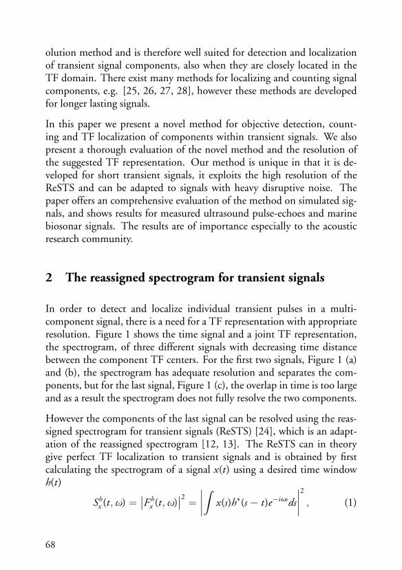
olution method and is therefore well suited for detection and localizationof transient signal components, also when they are closely located in theTF domain. There exist many methods for localizing and counting signalcomponents, e.g. [25, 26, 27, 28], however these methods are developedfor longer lasting signals.

In this paper we present a novel method for objective detection, count-ing and TF localization of components within transient signals. We alsopresent a thorough evaluation of the novel method and the resolution ofthe suggested TF representation. Our method is unique in that it is de-veloped for short transient signals, it exploits the high resolution of theReSTS and can be adapted to signals with heavy disruptive noise. Thepaper offers an comprehensive evaluation of the method on simulated sig-nals, and shows results for measured ultrasound pulse-echoes and marinebiosonar signals. The results are of importance especially to the acousticresearch community.

2 The reassigned spectrogram for transient signals

In order to detect and localize individual transient pulses in a multi-component signal, there is a need for a TF representation with appropriateresolution. Figure 1 shows the time signal and a joint TF representation,the spectrogram, of three different signals with decreasing time distancebetween the component TF centers. For the first two signals, Figure 1 (a)and (b), the spectrogram has adequate resolution and separates the com-ponents, but for the last signal, Figure 1 (c), the overlap in time is too largeand as a result the spectrogram does not fully resolve the two components.

However the components of the last signal can be resolved using the reas-signed spectrogram for transient signals (ReSTS) [24], which is an adapt-ation of the reassigned spectrogram [12, 13]. The ReSTS can in theorygive perfect TF localization to transient signals and is obtained by firstcalculating the spectrogram of a signal x(t) using a desired time windowh(t)

Shx (t,ω) =

∣∣F hx (t,ω)

∣∣2 = ∣∣∣∣∫ x(s)h∗(s − t)e−iωsds

∣∣∣∣2 , (1)

68

Figure 1: Illustration of a transient signal with two Gaussian pulses with differentTF centers; (a) pulses clearly separated in time and frequency; (b) pulses overlap-ping in time but clearly separated in frequency; (c) pulses overlapping so much intime that the frequency separation is not clear.

where ∗ denotes complex conjugate, ω = 2πf and the integral runs from−∞ to∞. The signal energy is then reassigned by introducing the reas-signment coordinates tx(t,ω) and ωx(t,ω) and the two-dimensional Diracimpulse,

∫ ∫f (t,ω)δ(t− t0,ω−ω0)dtdω = f (t0,ω0). The ReSTS is then

defined as

ReShx (t,ω) =

∫ ∫Sh

x (s, ξ)δ(t − tx(s, ξ),ω− ωx(s, ξ)

)dsdξ, (2)

and thus maps signal energy from a point (t0,ω0) to the point (tx(t0,ω0),ωx(t0,ω0)) in the spectrogram. The reassignment coordinates need to be

69

calculated for each selection of signal and time window according to

tx(t,ω) = t + ctR

(F th

x (t,ω)F h

x (t,ω)

),

ωx(t,ω) = ω− cωI(

F dh/dtx (t,ω)F h

x (t,ω)

),

(3)

where R and I represents the real and imaginary parts and F hx , F th

x andF dh/dt

x are the short-time Fourier transforms (STFTs) with different timewindows. The included scaling factors ct and cω makes the ReSTS ad-aptable to transient signals, and separates it from the normal reassignedspectrogram that have ct = cω = 1 [13, 24, 29].

Transient signals are often assumed to be Gaussian shaped in time, it isthus interesting to consider the unit energy Gaussian function

xG(t) = σ−1/2π−1/4e−

t2

2σ2 , (4)

and multi-component signals constructed by time, frequency and phaseshifted Gaussian shaped pulses

x(t) =K∑

k=1

akxG(t − tk)ei2πfktei2πφk , (5)

where ak is the amplitude, tk and fk = ωk/2π are the time and frequencycenters and φk ∈ [0 1) the phase shift.

Hansson-Sandsten and Brynolfsson [24] calculated the reassignment co-ordinates for a Gaussian signal with time-frequency center at the origin,and a matching Gaussian time window

txG (t,ω) = t − ctt2,

ωxG (t,ω) = ω− cωω

2.

(6)

Perfect TF localization is then achieved when ct = cω = 2, thus givingthe reassignment coordinates (txG (t,ω), ωxG (t,ω)) = (0, 0), i.e. the cor-rect time-frequency center. This result can easily be expanded to Gaussian

70

Figure 2: Illustration of the reassignment of signal energy and the resulting TFrepresentation, adapted for transient signals, for the signal in Figure 1 (c). Thesignal has two transient pulses which overlap heavily in time, however when thesignal energy is reassigned to the center of mass, the ReSTS shows two clear peaksat the correct TF centers.

signals with other TF centers since the spectrogram obeys time-frequencyshift-invariance and due to the linearity of the Fourier transform, the reas-signment coordinates are linear [29].

For multi-component signals (5), there will be some interaction betweenthe components after reassignment. However it is still possible for theReSTS to show clearly separated components, Figure 2, to be comparedwith the spectrogram in Figure 1 (c). The figure illustrates the reassign-ment of the signal energy to the new TF coordinates, according to (6)with ct = cω = 2, shown by the arrows in the spectrogram contour plotto the TF centers of the two pulses. The resulting ReSTS has two clearpeaks at the correct TF centers of the pulses and very little scattered signalenergy.

71

3 Automatic component detection algorithm

This section proposes an algorithm that automatically counts the numberof signal components in the ReSTS. The algorithm will enable users toautomatically find the number of transient pulses in a signal and the in-dividual TF locations of the pulses. It will thus be possible to objectivelyand efficiently analyze transient signals. To our knowledge there exist noresearched methods for finding multiple peaks in a matrix.

The ReSTS consists of high energy peaks in a low energy surrounding.Both signal components and noise will form peaks after the reassignment,however peaks will have more energy, and thus higher amplitude, if theyare the result of signal components. The algorithm therefore assumes thatany local maxima is a peak, either from a signal components or from noise,and that the amplitudes of the peaks will differ between signal componentsand noise.

A pseudo code of the proposed algorithm is presented. It uses the discretetime and discrete frequency ReSTS matrix, denoted ReS, as TF represent-ation. The user decides a maximum number of components for the signal,Kmax, the guess can be much larger than the expected number of compon-ents without compromising the performance, however very large numberswould increase the computational time. The user also sets an area arounda local maximum, 2δt wide in time and 2δf wide in frequency, that will beassumed not to include more than one local maximum. The choices of δt

and δf depend on the resolution of the ReSTS which will be evaluated inSection 4.1.

The constant 0 < ρ ≤ 1 is set by the user and allows the algorithm to beused for signals with relatively low SNR. Depending on the SNR, all noisepeak amplitudes could be low and relatively constant or some noise peakamplitudes could be rather high and close in amplitude to the signal peaks.A large ρ assumes high SNR, where signal and noise peak amplitudes areclearly separated, a small ρ assumes low SNR and allows the algorithm tofind relatively smaller signal peaks. The output from the algorithm is thetime locations T1,T2, . . . ,TK and the corresponding frequency locations,and F1, F2, . . . , FK , of the estimated signal peaks.

72

Algorithm 1 Pseudo codeInput: ReS, Kmax , δt , δf , ρOutput: T1,T2, . . . ,TK , F1, F2, . . . , FK

ReS : The ReSTS matrixKmax : Initial guess of maximum number of signal componentsδt : Smallest time separationδf : Smallest frequency separationρ : Normalizing constant for the noise amplitudesT1,T2, . . . ,TK : Time centers of the signal componentsF1, F2, . . . , FK : Frequency centers of the signal components

1: N = 3Kmax

2: for n=1:N do3: find coordinates of maximum in ReS, (T (n), F (n)4: save maximum amplitude in vector, A(n)5: define the rectangle area, BTF , with center (T (n), F (n)) and area 2δt ·2δf6: set the area BTF in ReS to 07: end for8: K = Kmax + 19: repeat

10: K = K − 111: Δn = ρ (A(K + 1)− A(N ))12: Δs = A(1)− A(K )13: Δ = A(K )− A(K + 1)14: if Δ > Δs then15: peak K is a signal component16: else if Δ < Δn then17: peak K is a noise component18: else19: if Δ/Δn > Δs/Δ then20: peak K is a signal component21: else22: peak K is a noise component23: end if24: end if25: until peak K is a signal component

73

The algorithm runs as described below:

• N = 3Kmax peaks are located to always include an adequate numberof noise peaks.

• The maximum peaks are estimated sequentially and the area of size2δt · 2δf around the current maximum peak is set to zero. Then thenext maximum peak can be located. The identified local maximaof the ReSTS can be assumed to be peaks because of the proper-ties of the ReSTS, and due to the structure of the algorithm, the Nidentified peaks are sorted with descending order of amplitude in allrelevant vectors.

• The number of assumed signal peaks among the N maximum peaksis set to K = Kmax + 1 and is then decreased with one for eachiteration the repeat loop. Δn is the difference in amplitude of allknown noise peaks, normalized with the constant ρ. Δs is the differ-ence in amplitude of all the possible signal peaks. Δ is the differencein amplitude of the smallest possible signal peak and largest knownnoise peak.

• In each iteration of the repeat loop (line 9 - 25), it is determinedif peak K is a signal or noise component. If peak K is determinedto be from a signal component, all peaks with larger amplitude areassumed to also be signal peaks and the algorithm has finished itssearch for signal peaks.

• Peak K will be determined to be from a signal or noise componentdepending on how much its amplitude deviates from the amplitudeslope created by the known noise peaks.

• If the testΔ > Δs (line 14) is passed, peak K should be a clear signalcomponent as its difference in amplitude to the largest noise peak islarger than its difference in amplitude to the largest identified peak.

• If the testΔ < Δn (line 16) is passed, peak K should be a noise peakas Δ will be relatively small.

• Note that bothΔ > Δs andΔ < Δn can be true, then peak K is as-sumed to be from a signal component, however the SNR is probablyvery low for such a signal.

74

• If none of the testΔ > Δs andΔ < Δn are true, then bothΔ/Δn ≥1 andΔs/Δ ≥ 1. The testΔ/Δn > Δs/Δ (line 19) is true ifΔs/Δis closer to 1 compared to Δ/Δn. This means that the amplitudeof peak K deviates from the amplitude slope of the noise peaks, andpeak K is assumed to be a signal component.

4 Resolution of the reassigned spectrogram for transientsignals

The proposed automatic component detection algorithm is designed to beused with the ReSTS, which means that the TF resolution of the ReSTSis of importance. In theory the ReSTS with Gaussian window can giveperfect TF localization to Gaussian signal components, however the resol-ution of components in signals disrupted by noise needs to be evaluated inorder for the proposed algorithm to be usable in practice.

We consider the signal x(t) in (5) that is a linear combination of Gaus-sian pulses (4) and add white Gaussian noise. For such a signal with twocomponents, that have the same frequency centers and amplitudes, butdifferent time centers, the components can be moved closer together intime to examine when different TF distributions no longer can resolve thecomponents.

In this section the simulated signals have sampling frequency 100 MHzand the scaling of the Gaussian pulses (4), σ = 0.5 μs, which gives anapproximate signal length of 1.2 μs, full width at half maximum, or ap-proximately 5 periods. The evaluated time distances range from to 0.5 μsto 2.0 μs, this means that the signal components will heavily overlap forsome test signals. White noise is additively disturbing the signals, withSNR = 5 dB, defined as averaged total signal energy to variance of thenoise.

Figure 3 shows a realization of the signal when (t1, t2) = (4.00, 5.50) μsand it can be seen that for this noisy signal, the overlap of the componentsis noticeable in time, Figure 3 (a), as well as in the spectrogram, Figure3 (b) and in the Choi-Williams distribution (CWD), [30], Figure 3 (c).

75

Figure 3: Illustrations for a realization of the simulated signal (5) with (t1, t2) =(4.00, 5.50) μs, white Gaussian noise and SNR = 5 dB; (a) the time signal; (b)the spectrogram; (c) the Choi-Williams distribution; (d) the ReSTS.

However, in the ReSTS, Figure 3 (d), the components are clearly separ-ated, showing the TF centers as clear peaks. Important to note is that thescaling parameter for the CWD, α = 0.2, is evaluated and chosen so thatit balances the suppression of interference and loss of resolution.

The three different TF distributions, the spectrogram and the ReSTS witha matched Gaussian window, σ = 0.50 μs, and the CWD, are evalu-ated by simulating 200 realizations of each test signal with different timedistances between components. Each simulation has different noise dis-turbance realizations and phase shifts for both signal components. The TFdistributions are calculated for each realization and the maximum in an

76

Table 1: Mean and standard deviation of the estimated time centers from 200simulations of the signal (5) with white Gaussian noise, SNR = 5 dB and randomphase for each pulse.

Spectrogram CWDMean [μs] SD [μs] Mean [μs] SD [μs]

Test True (t1, t2) t1 t2 t1 t2 t1 t2 t1 t2

1 (4.00, 6.00) μs 4.01 5.99 0.03 0.03 4.08 5.93 0.05 0.062 (4.00, 5.50) μs 4.12 5.37 0.19 0.21 4.13 5.37 0.11 0.103 (4.00, 5.00) μs 4.37 4.63 0.24 0.24 4.23 4.78 0.22 0.214 (4.00, 4.50) μs 4.23 4.26 0.07 0.07 4.14 4.35 0.16 0.15

ReSTSMean [μs] SD [μs]

Test True (t1, t2) t1 t2 t1 t2

1 (4.00, 6.00) μs 4.00 6.00 0.02 0.022 (4.00, 5.50) μs 4.01 5.50 0.04 0.043 (4.00, 5.00) μs 4.02 4.97 0.09 0.104 (4.00, 4.50) μs 4.14 4.35 0.12 0.12

area around the true TF center for both components are extracted to cal-culate the mean estimated TF centers and mean peak amplitudes. Theseresults are shown in Tables 1 - 2, where the standard deviation (SD) of theestimated time and frequency centers and coefficient of variation (CV) ofthe amplitudes are calculated to show the spread of the estimates and peakamplitudes.

It can be seen that all three methods separate the signal components whentime distance between the components is 2.00 μs, even though the CWDgives some deviations in the time centers, see Table 1. When the timedistance is 1.50 μs the spectrogram and the CWD are not able to givethe correct time centers, while the ReSTS gives a good estimate mean andlow standard deviation. This means that for this type of signal with lowSNR and random phase shifts, the spectrogram does not succeed to resolvethe Gaussian pulses that are 2σ = 1.0 μs apart, which is the theoreticalminimum time separation needed between two Gaussian pulses for thepeaks to be resolved [31]. The estimated time centers for the ReSTS are

77

Table 2: Mean and coefficient of variation of the peak amplitudes from 200 sim-ulations of the signal (5) with white Gaussian noise, SNR = 5 dB and randomphase for each pulse.

Spectrogram CWDMean CV Mean CV

Test A1 A2 A1 A2 A1 A2 A1 A2

1 89 89 0.04 0.04 192 192 0.11 0.112 95 95 0.18 0.18 201 201 0.19 0.193 131 131 0.45 0.45 227 227 0.40 0.404 169 169 0.61 0.61 268 269 0.61 0.61

ReSTSMean CV

Test A1 A2 A1 A2

1 3056 3177 0.33 0.342 1079 1077 0.36 0.323 384 366 0.48 0.444 1250 1310 1.07 1.08

however still very good when (t1, t2) = (4.00, 5.00) μs, it is not until thetime distance is 0.5 μs that the estimates for the ReSTS becomes unreliable.

The signal peak amplitudes of the ReSTS are much higher compared tothe other TF distributions, Table 2. This clearly shows that the signal en-ergy is more localized to the TF centers of each component in the ReSTScompared to both the spectrogram and CWD. The peak amplitudes in thespectrogram and CWD increase when the component separation decrease,and the energy from the components combine. The amplitudes in theReSTS first decrease because reassignment to the correct mass centers be-comes more difficult for closer components, and some energy is reassignedto positions in between the true TF centers. For the smallest time distance,the ReSTS is unreliable and sometimes only gives one strong peak, result-ing in high mean amplitude but also very high coefficient of variation.

The estimated frequency centers are not presented, as all methods havegood estimations for these signals. This is expected, since the signal com-ponents have the same frequency, and thus any smoothing of the TF dis-tributions will be mainly in the time domain.

78

4.1 Guidance in parameter choices of δt and δf

The proposed automatic component detection algorithm requires the userto define the parameters δt and δf , which are signal dependent. Findingtheoretical values for these parameters is an arduous task because of the in-teraction between close signal components and noise in the ReSTS. Valuescan instead be found experimentally and be translated to a general signal.

To achieve the best performance of the proposed automatic componentdetection algorithm together with the ReSTS, the parameters δt and δf

should be defined equal to the time and frequency resolution of the ReSTS.The algorithm will then be able to both resolve, and thus accurately detect,any two components which are separated by at least δt and δf . We are alsointerested in results that can be applied to real, measured signals, thereforethis section will experimentally find the resolution of the ReSTS for noisy,transient signals.

According to the Heisenberg inequality, even the most optimal resolutionneed to fulfill, δtδf ≥ 1/(4π), where δt is the uncertainty in time, i.e. thelength of the pulse, and δf is the uncertainty in frequency. Two Gaussianpulses of equal amplitude and time length, are separable if

δt[s] = 2σ[s], δf [s−1] = 1/(πσ[s]), (7)

where σ is the scaling parameter of the Gaussian [31]. This means thatthese distances correspond to the best resolution the spectrogram can pos-sibly achieve.

Defining the signals as in (5) with two Gaussian pulse components andchanging the TF center of one component, the minimum time and fre-quency distances needed to resolve two components for the ReSTS canbe determined. For the used test signals the Gaussian pulses have σ =0.50 μs, the sampling frequency is 100 MHz and 0.01 μs corresponds to1 sample. The simulated signals are disturbed by white Gaussian noise,SNR = 5 dB, which will give δt and δf that can be used when applying theautomatic component detection method on measured data, possibly alsowith severe disrupting noise.

79

Figure 4: Realizations of the test signals (5) with two Gaussian pulses and whiteGaussian noise, SNR = 5 dB, where f1 = f2 = 4.00 MHz and random phases ofthe components. The time signal is shown to the left and the ReSTS is viewedso that the amplitude and time axes (middle) or amplitude and frequency axes(right) can be seen; (a) signal with (t1, t2) = (3.00, 4.10) μs; (b) signal with(t1, t2) = (3.00, 4.00) μs; (c) signal with (t1, t2) = (3.00, 3.90) μs; (d) signal with(t1, t2) = (3.00, 3.80) μs.

The minimum required time separation is evaluated by keeping the fre-quency of the two signal components constant and decreasing the timedistance between the TF centers of the components. Figure 4 shows real-izations of the signals with decreasing time separation of the TF centers,it shows the time signal (left) and the ReSTS from two viewpoints so thatonly the time (middle) or frequency (right) axis is seen. The figure showsthat the signal energy becomes more scattered, as it reassigns to locationsbetween the components, when the time distance decreases.

80

Table 3: Mean and standard deviation of the estimated time centers and the meanand coefficient variation of the peak amplitudes from 200 simulations of the signal(5) with f1 = f2 = 4.00 MHz, white Gaussian noise, SNR = 5 dB and randomphase for each pulse.

Mean [μs] SD [μs] Mean CVTrue (t1, t2) t1 t2 t1 t2 A1 A2 A1 A2

(3.00, 4.10) μs 3.03 4.08 0.08 0.07 6764 6667 0.41 0.38(3.00, 4.00) μs 3.04 3.97 0.09 0.09 5758 5695 0.47 0.40(3.00, 3.90) μs 3.06 3.84 0.11 0.11 5314 5261 0.54 0.52(3.00, 3.80) μs 3.06 3.73 0.12 0.14 5169 5350 0.59 0.67

Table 3 shows the results of 200 simulations of the test signals, with ran-dom noise and phase shift of the components for each simulation. Thetable only shows the estimated time centers and peak amplitudes, since theestimated frequency centers are consistently reliable for all time distances.It can be seen that the mean estimates differ at most 6 samples from thetrue positions, however when t2 = 3.90 μs the mean of t2 is closer to3.80 μs than the true value. Also when the time distance is less than 1.0 μsthe coefficient variations of the peak amplitudes are more than 50%, whichindicates that the signal energy can be rather scattered, as can be seen inFigure 4 (c) and (d). It can therefore be safer to set δt corresponding to1.0 μs even though the estimated time centers for the smaller time dis-tances are close to the truth. For the chosen signals of this experiment,1.0 μs corresponds to 2σ, which then can be applied to a general Gaussianpulse, multi-component, transient signal.

The required minimum frequency distance between two components is ex-amined by keeping the time centers of the two signal components constantand decreasing the frequency distance between the TF centers of the com-ponents. Again, σ = 0.50 μs and the sampling frequency is 100 MHz. Forthe calculated ReSTS matrices, the distance between two frequency valuesis 0.012 MHz.

Figure 5 shows realizations of the simulated signals for each of the fourchosen frequency separations. The figure shows the time signal and theReSTS, first the time signal (left) and then ReSTS from two viewpoints

81

Figure 5: Realizations of the test signals (5) with two Gaussian pulses and whiteGaussian noise, SNR = 5 dB, where t1 = t2 = 3.00 μs and random phase ofthe components. The time signal is shown to the left and the ReSTS is viewedso that the amplitude and time axes (middle) or amplitude and frequency axes(right) can be seen; (a) signal with (f1, f2) = (4.00, 4.70) MHz; (b) signal with(f1, f2) = (4.00, 4.65) MHz; (c) signal with (f1, f2) = (4.00, 4.60) MHz; (d)signal with (f1, f2) = (4.00, 4.55) MHz.

so that only the time (middle) or frequency (right) axis is seen. It can benoted that the energy seem more scattered for smaller frequency distances.

Table 4 shows the estimated frequency centers and peak amplitudes from200 simulations of the test signals, where the noise and phase shifts of thecomponents are random for each simulation. The estimated time centerswere all consistent and close to the true value t1 = t2 = 3.00 μs. It can beseen that the estimated frequency centers over all are reliable, the mean ofthe estimates deviates at most 4 samples from the true frequency centers.The standard deviations for the estimated frequency centers are also rather

82

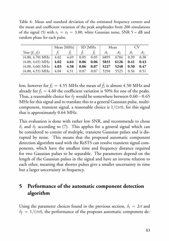
Table 4: Mean and standard deviation of the estimated frequency centers andthe mean and coefficient variation of the peak amplitudes from 200 simulationsof the signal (5) with t1 = t2 = 3.00, white Gaussian noise, SNR 5 = dB andrandom phase for each pulse.

Mean [MHz] SD [MHz Mean CVTrue (f1, f2) f1 f2 f1 f2 A1 A2 A1 A2

(4.00, 4.70) MHz 4.02 4.69 0.05 0.05 6895 6704 0.39 0.38(4.00, 4.65) MHz 4.02 4.64 0.06 0.06 5831 6126 0.41 0.43(4.00, 4.60) MHz 4.03 4.58 0.06 0.07 5227 5248 0.50 0.47(4.00, 4.55) MHz 4.04 4.51 0.07 0.07 5294 5525 0.56 0.51

low, however for f2 = 4.55 MHz the mean of f2 is almost 4.50 MHz andalready for f2 = 4.60 the coefficient variation is 50% for one of the peaks.Thus, a reasonable choice for δf would be somewhere between 0.60−0.65MHz for this signal and to translate this to a general Gaussian pulse, multi-component, transient signal, a reasonable choice is 1/(πσ), for this signalthat is approximately 0.64 MHz.

This evaluation is done with rather low SNR, and recommends to choseδt and δf according to (7). This applies for a general signal which canbe considered to consist of multiple, transient Gaussian pulses and is dis-rupted by noise. This means that the proposed automatic componentdetection algorithm used with the ReSTS can resolve transient signal com-ponents, which have the smallest time and frequency distance requiredfor two Gaussian pulses to be separable. The parameters depend on thelength of the Gaussian pulses in the signal and have an inverse relation toeach other, meaning that shorter pulses give a smaller uncertainty in timebut a larger uncertainty in frequency.

5 Performance of the automatic component detectionalgorithm

Using the parameter choices found in the previous section, δt = 2σ andδf = 1/(πσ), the performance of the proposes automatic component de-

83

tection algorithm can now be evaluated. This is done using test signals(5) with the different number of components, TF centers and amplitudesgiven in Table 5. Two multi-component signals are used, one with twoand one with five components. The first two presented in Table 5 formsthe two-component signal and the five-component signal includes all five.

The test signals are evaluated with SNR = 5 dB and SNR = 15 dB, where500 simulations are done for each signal and SNR, with different noiserealizations and random phase shifts for the signal components. Thesampling frequency is 100 MHz and the scaling of the Gaussian pulsesσ = 0.5 μs. The automatic algorithm extracts Kmax peaks of the ReSTSand determines which peaks that are signal components.

For the evaluation a detection rate is calculated, giving a value 0 - 1. If thealgorithm finds the correct number of signal components, which all areclose to the true TF centers, then the detection is considered correct (1).In all other cases the detection is incorrect (0). The correct and incorrectdetections from the 500 simulations are averaged to get the detection rate.Thus 1 means that detection was correct for all 500 simulations and 0 thatdetection was incorrect for all simulations.

Table 6 shows the resulting detection rates for six tests. For all tests withtwo signal components, the maximum number of peaks parameter ischosen to Kmax = 5 and when the signal has five components Kmax = 8.An estimated TF center is considered close enough to the true TF cen-

Table 5: Time and frequency centers and amplitudes for the transient, multi-component Gaussian signal (5), used for evaluating the performance of the pro-posed automatic component detection algorithm.

k tk [μs] fk [MHz] ak

1 3.0 2.0 1.02 5.0 5.0 0.63 3.0 8.0 0.84 7.0 2.0 0.65 7.0 8.0 0.4

84

Table 6: Detection rate of the automatic component detection algorithm formulti-component, transient signals (5), disturbed by white noise and with para-meters according to Table 5. The detection rates are obtained from 500 simu-lations with different noise realizations and where the signal components haverandom phase shifts. If all detections for all 500 simulations are correct, the rateis 1.

Detection rate forSNR [dB] ρ 2 components 5 components

15 2/3 1 15 2/3 1 0.955 1/3 1 0.98

ter if the time and frequency difference is less than δt = 2σ = 1 μs andδf = 1/(πσ) = 0.65 MHz respectively.

It can be seen in Table 6 that for the signals with two components, theproposed algorithm always detects the correct signal components. For thesignals with five components, the detection rate is 0.95 when the SNRis low, however the result can be improved to 0.98 by lowering the nor-malization constant ρ. When the SNR is higher, the algorithm correctlyidentifies all components even for the five components signals.

Since there, to our knowledge, exist no other researched methods, the per-formance of our algorithm can not be compared to other known methods.However when considering the ReSTS matrix, two other, perhaps simpler,approaches seem natural. The first approach is to calculate some thresholdfor the noise peak amplitudes. The distribution of the (scaled reassigned)noise peaks is unknown, however a threshold based on the Gaussian distri-bution might be reasonable, or the universal threshold for noise reductionusing discrete Wavelet transform [32]. The second approach is to look atthe peaks sequentially from the largest peak and continue until the peakamplitudes drop and then level out, the peaks after the drop will then beassumed to be noise peaks.

We have implemented such schemes and evaluated the detection rate forthe same test signals used previously. The Wavelet universal threshold gives

85

a detection rate around 0.90, however the detection rate decreases whenSNR increases, which certainly is undesirable. The Gaussian threshold,has detection rates around 0.25 - 0.30, which also decreases when SNRincreases. The level out approach has a detection rate around 0.60 for thesignals with two components and approximately 0.50 for the signals withfive components.

6 Examples on measured data

This section shows how the proposed automatic component detection al-gorithm performs on real, measured signals, from two acoustic fields. Be-fore using the method on measured data, the time window length of theReSTS needs to be decided. The time window should have the same lengthas, e.g. time duration of, the transient signal components. If the timeduration is not known, an appropriate length of the time window can bedetermined by evaluating the local Renyi entropy of the ReSTS for dif-ferent lengths of the time window [24]. When an appropriate length isused, the energy concentration will be high and accordingly the Renyi en-tropy small. It is not essential that the length of the time window exactlymatches the duration of the transient signal components, the ReSTS isstable for different window lengths.

6.1 Ultrasound pulse-echo measurements

The automatic component detection algorithm was tested on real meas-urements from a simple pulse-echo measurement setup in water. A 2.1MHz in-house built transducer functioned as both sender and receiver.An ultrasonic pulse was generated using a Panametrix Pulse/receiver Model5072PR device and was measured at 100 MHz sampling rate with a Tex-tronix TDS 2002C oscilloscope. The reflective object was a plexi glassphantom with the shape of a solid stairway with step sizes ranging from 2mm to 0.25 mm. A sketch of the phantom can be seen in Figure 6.

Measurements were taken in each transition between two steps of the plexiglass phantom. This resulted in a total of four measured time signals con-

86

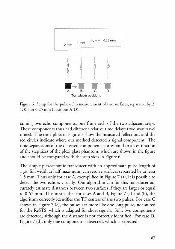
2 mm 1 mm 0.5 mm 0.25 mm

Transducer positionsA. B. C. D.

Figure 6: Setup for the pulse-echo measurement of two surfaces, separated by 2,1, 0.5 or 0.25 mm (positions A-D).

taining two echo components, one from each of the two adjacent steps.These components thus had different relative time delays (two way traveltimes). The time plots in Figure 7 show the measured reflections and thered circles indicate where our method detected a signal component. Thetime separations of the detected components correspond to an estimationof the step sizes of the plexi glass phantom, which are shown in the figureand should be compared with the step sizes in Figure 6.

The simple piezoceramic transducer with an approximate pulse length of1 μs, full width at half maximum, can resolve surfaces separated by at least1.5 mm. Thus only for case A, exemplified in Figure 7 (a), it is possible todetect the two echoes visually. Our algorithm can for this transducer ac-curately estimate distances between two surfaces if they are larger or equalto 0.67 mm. This means that for cases A and B, Figure 7 (a) and (b), thealgorithm correctly identifies the TF centers of the two pulses. For case Cshown in Figure 7 (c), the pulses act more like one long pulse, not suitedfor the ReSTS, which is adapted for short signals. Still, two componentsare detected, although the distance is not correctly identified. For case D,Figure 7 (d), only one component is detected, which is expected.

87

Figure 7: Time signals and peak detections from ReSTS, of pulse-echo measure-ments of two surfaces that are separated by 2, 1, 0.5 or 0.25 mm (a) - (d). Thered circles indicate the detected time centers, obtained by the automatic detectionmethod from the ReSTS. The time separation between the pulse centers corres-pond to an estimation of the step sizes of the plexi glass phantom, Figure 6. Theestimates are shown in red (above), the true step sizes are shown in black (under).

For our algorithm, the parameters were set to δt = 2σ = 0.9 μs, δf =1/(πσ) = 0.7 MHz, ρ = 1 and Kmax = 4. The length of the signal, andthus σ, could be estimated studying a single pulse using full width at halfmaximum. It is important to note that while we choose to use σ = 0.45 μs,equivalent results were obtained for σ ∈ [0.38 0.65] μs. Thus for thesesignals our method is robust to choices of σ.

88

Figure 8: Two dolphin echolocation signals, to the left a bimodal, to the right aunimodal; (a) time signal; (b) spectrogram; (c) ReSTS representation and detectedsignal TF centers; (d) pulse detections.

6.2 Marine biosonar signals

The usefulness of the developed automatic component detection algorithmis further exemplified by applying it to recorded dolphin echolocation sig-nals. Recordings were made from different parts of the echolocation beammain lobe. Details regarding how these recordings were made are explainedby Starkhammar et al. [10].

Figure 8 left hand side, shows recordings from a bimodal transient signal,expected to contain more than one component. Figure 8 right hand side,shows recordings from a unimodal transient signal, expected to containonly one component. The algorithm outcome in Figure 8 (left) shows that

89

it detects two signal components separated in both time and frequency,while in Figure 8 (right) only one component is detected.

For the ReSTS and the automatic component detection algorithm, σ =6.4 μs, Kmax = 3 and ρ = 2/3 are used. This means that the resolutionin time is δt = 2σ = 13 μs and in frequency δf = 1/(πσ) = 53 kHz.However similar results are obtained for σ ∈ [5 8] μs, so our method isrobust to choices of σ for these signals.

From a biosonar perspective, it is interesting to compare the signal com-ponent time and frequency centers in Figure 8. Although such a compar-ison lies outside the scope of this paper, it brings new information andinsights to how the different parts of the echolocation beam of bottle nosedolphins (Tursiops truncatus) are generated in terms of suggested internalfrequency filters, acoustic reflection pathways and possibly multiple echo-location sources [9, 10, 33, 34].

7 Conclusions

In this paper an automatic component detection method for short, multi-component transient signals has been proposed. The method combines anovel detection algorithm with a high-resolution TF representation adap-ted for short transient signals, ReSTS. As a result, the method automat-ically counts, the beforehand unknown, number of transient componentsand estimates the TF centers of individual components with great preci-sion. The results are also easily visualized by the ReSTS, showing the TFcenters of individual components, marked by the automatic algorithm.

Our proposed automatic component detection algorithm and TF rep-resentation are useful for severely coinciding Gaussian shaped transients,where other comparable methods fail to resolve the components. The res-olution of the suggested TF representation is shown to be the best achiev-able for Gaussian shaped pulses. In addition, the calculations of time andfrequency centers of the components are robust to noise. The method iseasy to use since the algorithm requires very little user input. The paper

90

provides guidelines on how to choose the input parameters, although themethod is quite insensitive to parameter choices.

This new method should be useful in several acoustic research fields, notthe least sonar and biosonar applications, or other fields where coincidingGaussian shaped transients are analyzed. In this paper the method showspromising results on measured data, both from a laboratory pulse-echoset-up and a dolphin echolocation signal measured simultaneously at twodifferent locations in the echolocation beam. The method resolves heavilyoverlapping pulses from the pulse-echo signals and automatically detectsthe expected number of components in the bimodal and unimodal echo-location signal.

Acknowledgments

The authors would like to thank the Navy Marine Mammal Program andDorian S. Houser, Patrick W. Moore and Lois Talmadge, National MarineMammal foundation, USA, for their generous contribution of dolphinecholocation data. The research reported in this paper was supported bythe Swedish Research Council.

91

References

[1] C. Wei, W. W. L. Au, D. R. Ketten, Z. Song, and Y. Zhang,“Biosonar signal propagation in the harbor porpoise’s (Phocoenaphocoena) head: The role of various structures in the formation ofthe vertical beam.,” Journal of the Acoustical Society of America, vol.141, no. 6, pp. 4179, 2017.

[2] C. Capus, Y. Pailhas, K. Brown, D.M. Lane, P. Moore, andD. Houser, “Bio-inspired wideband sonar signals based on obser-vations of the bottlenose dolphin (Tursiops truncatus),” J. Acoust.Soc. Am., vol. 121, no. 1, pp. 594–604, 2007.

[3] J. Pons-Llinares, M. Riera-Guasp, J. A. Antonino-Daviu, and T. G.Habetler, “Pursuing optimal electric machines transient diagnosis:The adaptive slope transform.,” Mechanical Systems and Signal Pro-cessing, vol. 80, pp. 553 – 569, 2016.

[4] Q. He and X. Ding, “Sparse representation based on local time-frequency template matching for bearing transient fault feature ex-traction.,” Journal of Sound and Vibration, vol. 370, pp. 424 – 443,2016.

[5] H. Liu, W. Huang, S. Wang, and Z. Zhu, “Adaptive spectral kurtosisfiltering based on morlet wavelet and its application for signal transi-ents detection.,” Signal Processing, vol. 96, no. Part A, pp. 118 – 124,2014.

[6] L. Cohen, Time-Frequency Analysis, Signal Processing Series.Prentice-Hall, Upper Saddle River, NJ, USA, 1995.

93

[7] W. W. L. Au, “Echolocation signals of the atlantic bottlenose dol-phin (tursiops truncatus) in open waters,” in Animal Sonar Systems,Rene-Guy Busnel and James F. Fish, Eds., pp. 251–282. SpringerUS, Boston, MA, 1980.

[8] W. W. L. Au, The Sonar of Dolphins, Springer-Verlag, 1993.

[9] W. W. L. Au, B. Branstetter, P.W. Moore, and J.J. Finneran, “Dol-phin biosonar signals measured at extreme off-axis angles: Insights tosound propagation in the head,” J. Acoust. Soc. Am., vol. 132, no. 2,pp. 1199–1206, 2012.

[10] J. Starkhammar, P.W.B. Moore, L. Talmadge, and D.S. Houser,“Frequency-dependent variation in the two-dimensional beam pat-tern of an echolocating dolphin,” Biol. Lett., vol. 7, no. 6, pp. 836–839, 2011.

[11] S. Wang, S. Huang, Q. Wang, Y. Zhang, and W. Zhao, “Modeidentification of broadband Lamb wave signal with squeezed wavelettransform.,” Applied Acoustics, vol. 125, pp. 91 – 101, 2017.

[12] K. Kodera, C. de Villedary, and R. Gendrin, “A new method for thenumerical analysis of nonstationary signals,” Physics of the Earth &Planetary Interiors, vol. 12, pp. 142–150, 1976.

[13] F. Auger and P. Flandrin, “Improving the readability of time-frequency and time-scale representations by the reassignmentmethod,” IEEE Trans. on Signal Processing, vol. 43, pp. 1068–1089,May 1995.

[14] I. Daubechies, J. Lu, and H.-T. Wu, “Synchrosqueezed wavelettransforms: An empirical mode decomposition-like tool.,” Applied& Computational Harmonic Analysis, vol. 30, no. 2, pp. 243 – 261,2011.

[15] N. E. Huang and Z. Wu, “A review on Hilbert-Huang transform:Method and its applications to geophysical studies,” Reviews of Geo-physics, vol. 46, no. 2, pp. n/a–n/a, 2008, RG2006.

94

[16] S. Wang, X. Chen, Y. Wang, G. Cai, B. Ding, and X. Zhang, “Non-linear squeezing time-frequency transform for weak signal detection,”Signal Processing, vol. 113, pp. 195–210, August 2015.

[17] H. Guo, “A simple algorithm for fitting a Gaussian function [dsptips and tricks],” IEEE Signal Processing Magazine, vol. 28, no. 5, pp.134–137, Sept 2011.

[18] E. Kheirati Roonizi, “A new algorithm for fitting a Gaussian func-tion riding on the polynomial background.,” IEEE Signal ProcessingLetters, vol. 20, no. 11, pp. 1062 – 1065, 2013.

[19] S.C. Pei and S.G. Huang, “STFT with adaptive window width basedon the chirp rate,” IEEE Transactions on Signal Processing, vol. 60, no.8, pp. 4065 – 4080, 2012.

[20] S. Ghofrani, “Matching pursuit decomposition for high-resolutiondirection of arrival.,” Multidimensional Systems and Signal Processing,vol. 26, no. 3, pp. 693 – 716, 2015.

[21] P. Balazs, M. Dorfler, F. Jaillet, N. Holighaus, and G. Velasco,“Theory, implementation and applications of nonstationary Gaborframes.,” Journal of Computational and Applied Mathematics, vol.236, pp. 1481 – 1496, 2011.

[22] H. Kalbkhani and M. G. Shayesteh, “Stockwell transform for epi-leptic seizure detection from eeg signals.,” Biomedical Signal Pro-cessing and Control, vol. 38, pp. 108 – 118, 2017.

[23] M. Hamidia and A. Amrouche, “A new robust double-talk detectorbased on the Stockwell transform for acoustic echo cancellation.,”Digital Signal Processing, vol. 60, pp. 99 – 112, 2017.

[24] M. Hansson-Sandsten and J. Brynolfsson, “The scaled reassignedspectrogram with perfect localization for estimation of Gaussianfunctions,” IEEE Signal Processing Letters, vol. 22, no. 1, pp. 100–104, January 2015.

[25] I. Reinhold and M. Sandsten, “Optimal time-frequency distribu-tions using a novel signal adaptive method for automatic componentdetection,” Signal Processing, vol. 133, pp. 250 – 259, 2017.

95

[26] J. Lerga, V. Sucic, and B. Boashash, “An efficient algorithm for in-stantaneous frequency estimation of nonstationary multicomponentsignals in low SNR,” EURASIP Journal on Advances in Signal Pro-cessing, pp. 1–16, January 2011.

[27] B. Barkat and K. Abed-Meraim, “Algorithms for blind componentsseparation and extraction from the time-frequency distribution oftheir mixture,” EURASIP Journal on Applied Signal Processing, vol.13, pp. 2025–2033, 2004.

[28] L. A. Cirillo and M. G. Amin, “Auto-term detection using time-frequency array processing,” in IEEE International Conference onAcoustics, Speech, and Signal Processing, April 2003, vol. 6, pp. VI–465–VI–468.

[29] E. Chassande-Mottin, F. Auger, and P. Flandrin, “Reassignment,” inTime-Frequency Analysis, F. Hlawatsch and F. Auger, Eds., chapter 9,pp. 249–277. U.K.: ISTE, London, 2008.

[30] H.I. Choi and W. J. Williams, “Improved time-frequency represent-ation of multi-component signals using exponential kernels,” IEEETrans. Acoustics, Speech and Signal Processing, vol. 37, pp. 862–871,June 1989.

[31] H. Holzmann and S. Vollmer, “A likelihood ratio test for bimodalityin two-component mixtures with application to regional income dis-tribution in the EU,” AStA Advances in Statistical Analysis, vol. 92,no. 1, pp. 57–69, Feb 2008.

[32] D. B. Percival and A. T. Walden, Wavelet Methods for Time SeriesAnalysis, Cambridge University Press, Cambridge, United Kingdom,July 2000.

[33] T. W. Cranford, W. R. Elsberry, W. G. Van Bonn, J. A. Jeffress, M. S.Chaplin, D. J. Blackwood, D. A. Carder, T. Kamolnick, M. A. Todd,and S. H. Ridgway, “Observation and analysis of sonar signal genera-tion in the bottlenose dolphin (tursiops truncatus): Evidence for twosonar sources,” Journal of Experimental Marine Biology and Ecology,vol. 407, no. 1, pp. 81 – 96, 2011.

96

[34] P. T. Madsen, M. Lammers, D. Wisniewska, and K. Beedholm,“Nasal sound production in echolocating delphinids (tursiops trun-catus and pseudorca crassidens) is dynamic, but unilateral: clickingon the right side and whistling on the left side,” Journal of Experi-mental Biology, vol. 216, no. 21, pp. 4091–4102, 2013.

97

Paper C

Paper C

The scaled reassigned spectrogram adaptedfor detection and localisation of transientsignals

Isabella Reinhold1, Josefin Starkhammar2, Maria Sandsten1

1Mathematical Statistics, Centre for Mathematical Sciences, Lund University,Sweden.

2Department of Biomedical Engineering, Lund University, Sweden.

Abstract

The reassigned spectrogram can be used to improve the readability of atime-frequency representation of a non-stationary and multi-componentsignal. However for transient signals the reassignment needs to be adap-ted in order to achieve good localisation of the signal components. Oneapproach is to scale the reassignment. This paper shows that by adaptingthe shape of the time window used with the spectrogram and by scalingthe reassignment, perfect localisation can be achieved for a transient sig-nal component. It is also shown that without matching the shape of thewindow, perfect localisation is not achieved. This is used to both identifythe time-frequency centres of components in a multi-component signal,and to detect the shapes of the signal components. The scaled reassignedspectrogram with the matching shape window is shown to be able to re-solve close components and works well for multi-components signals withnoise. An echolocation signal from a beluga whale (Delphinapterus leucas)provides an example of how the method performs on a measured signal.

Keywords: Hermite functions, non-stationary signals, time-frequencyanalysis, reassignment, signal resolution

101

1 Introduction

For non-stationary signals the reassigned spectrogram (Re-Spect) can im-prove the readability of the time-frequency representation [1, 2]. The con-centration of a component is increased by reassigning mass to the centreof gravity, squeezing the signal terms to be more localised, while cross-terms are reduced by a smoothing of the specific distribution. Recently, thetheoretical expressions for the reassigned Gabor spectrograms of Hermitefunctions have been derived [3, 4]. Although the Re-Spect gives perfectlocalisation of linear chirps, this is not achieved for transient signals whichare common in for example marine biosonar research. Transient signalscan effectively be modelled by a linear combination of Hermite basis func-tions [5, 6, 7, 8]. Perfect localisation of a Gaussian function (first Hermitefunction) can be achieved by the adaptable reassignment methods, theLevenberg-Marquardt reassignment [9] and the scaled reassigned spectro-gram (ScRe-Spect) [10].

This paper builds on the ScRe-Spect to show that perfect localisation intime and frequency can be achieved with reassignment for higher orderHermite functions. Perfect localisation is possible if the shape of the timewindow used with the spectrogram is matched with the shape of the signalcomponent. It also shows that when the matching shape window is notused, perfect localisation is not possible with the ScRe-Spect. This canbe used to detect the shape of and localise the time-frequency centres ofindividual transient components in a non-stationary signal.

To illustrate the use of the ScRe-Spect with matching shape window thispaper includes an example of an echolocation signal from a beluga whale(Delphinapterus leucas). In this field, there is a need for signal processingmethods that allows for analysis of the time dependence of each frequencycomponent within each echolocation signal [11, 12, 13].

In this paper, section 2 calculates the reassignment coordinates for firstand second Hermite signal components with first and second Hermitetime windows. The results are also extended to multi-component sig-nals. The performance of the ScRe-Spect is evaluated in section 3, bysimulating transient multi-component signals with noise. Section 4 shows

102

the performance of the method on a measured echolocation signal from adolphin. Section 5 concludes the paper.

2 The scaled reassigned spectrogram

The spectrogram of the signal x(t) using the window h(t) is found fromthe short-time Fourier transform (STFT)

Shx (t,ω) =

∣∣F hx (t,ω)

∣∣2 = ∣∣∣∣∫ x(s)h∗(s − t)e−iωsds

∣∣∣∣2 . (1)

The Re-Spect, with reassignment to tx and ωx, is defined as

RShx (t,ω) =

∫ ∫Sh

x (s, ξ)δ(t − tx(s, ξ),ω− ωx(s, ξ)

)dsdξ, (2)

where δ(t,ω) is the two-dimensional Dirac impulse defined as∫ ∫f (t,ω)δ(t − t0,ω− ω0)dtdω = f (t0,ω0). (3)

As shown in [10], the scaling factors ct and cω can be introduced and thereassignment coordinates can be computed as

tx(t,ω) = t + ctR

(F th

x (t,ω)F h

x (t,ω)

),

ωx(t,ω) = ω− cωI(

F dh/dtx (t,ω)F h

x (t,ω)

),

(4)

where R and I are the real and imaginary parts respectively and F hx , F th

xand F dh/dt

x are STFTs with different time windows. If ct = cω = 1 the Re-Spect is obtained [4, 14]. Since the reassignment coordinates are calculatedfrom STFTs using the same signal values needed for the spectrogram andonly differs in the choice of time window, the computational complexityof the ScRe-Spect is not drastically increased compared the spectrogram.

103

2.1 The scaled reassigned spectrogram of multi-component transientsignals

A multi-component transient signal can be modelled as a sum of Hermitefunctions

x(t) =n∑

k=1

akxk(t − tk)eiωkt , (5)

where xk(t) are Hermite basis functions, tk and ωk are the time and fre-quency centres and ak the amplitudes. Due to the linearity of the Fouriertransform, the reassignment vector is also linear [14]. For the calculationsit is assumed that the reassignment can be calculated for each componentindividually. This is true for a signal with somewhat separated compon-ents, in time or frequency. The spectrogram also obeys time-frequencyshift-invariance, meaning that further analysis can be restricted to signalsof the form xk(t) = gk(t) instead of xk(t) = gk(t − tk)e−iωkt .

This paper analyses the unit energy Gaussian function

x1(t) = σ−1/2π−1/4e−

t2

2σ2 , (6)

and the unit energy second Hermite function

x2(t) = 21/2σ−3/2π−1/4te−

t2

2σ2 , (7)

as the amplitude of the signal has no effect on the reassignment coordin-ates, compare (4). The ScRe-Spect with perfect localisation of x1(t) usinga Gaussian window is shown in [10]. The next section will show thatthe ScRe-Spect of a signal x(t) = x1(t) + x2(t) with a Gaussian windowwill only give perfect localisation to x1(t) while the energy of x2(t) remainsscattered, and when a second Hermite window is used, perfect localisationwill be obtained for x2(t) but not for x1(t).

104

2.2 Scaled reassignment with a Gaussian window

The reassignment coordinates for x1(t) using a window h1(t) = x1(t),where the window and signal have the same time length, are

th1x1

(t,ω) = t − ctt2,

ωh1x1

(t,ω) = ω− cωω

2,

(8)

and perfect localisation is achieved when ct = cω = 2 [10]. To find thereassignment coordinates for x2(t) with h1(t), we need to calculate the ne-cessary STFTs, also assuming that the time length of the signal and windoware the same

F h1x2

(t,ω) =

√2

σ2√π

∫se−(s2+(s−t)2)/(2σ2)e−iωsds

=

√2

σ2√π

e−t2/(2σ2)

∫se−s2/σ2+(t/σ2−iω)sds

=t − iσ2

ω√2σ

e−(t2/σ2+σ2ω

2+i2tω)/4,

(9)

F th1x2

(t,ω) =

√2

σ2√π

∫s(s − t)e−(s2+(s−t)2)/(2σ2)e−iωsds

=2σ2 − t2 − σ4

ω2

2√

2σe−(t2/σ2+σ2

ω2+i2tω)/4.

(10)

The derivative of h1(t) is dh1(t)/dt = −th1(t)/σ2, thus

F dh1/dtx2

(t,ω) = − 1σ2

F th1x2

(t,ω). (11)

This gives the reassignment coordinates

th1x2

(t,ω) = t − ct

(t2− σ

2tt2 + σ4ω2

),

ωh1x2

(t,ω) = ω− cω

(ω

2− σ

2ω

t2 + σ4ω

).

(12)

105

It can be seen that there exist no ct or cω so that(th1x2

(t,ω), ωh1x2

(t,ω))=

(0, 0), i.e. the centre of the component, ∀ t,ω. Instead of perfect local-isation of the component x2(t), the reassigned energy will be located onellipses, which is also found for the reassigned Gabor spectrogram in [4].

2.3 Scaled reassignment with a second Hermite window

Using the second Hermite window, h2(t) = x2(t), with the spectrogram,makes it possible to get perfect localisation to x2(t) with scaled reassign-ment. For the calculations of the reassignment coordinates it is assumedthat the time length of the window is the same as for the signal,

F h2x2

(t,ω) =2σ3√π

∫s(s − t)e−(s2+(s−t)2)/(2σ2)e−iωsds

=2σ2 − t2 − σ4

ω2

2σ2e−(t2/σ2+σ2

ω2+i2tω)/4,

(13)

F th2x2

(t,ω) =2σ3√π

∫s(s − t)2e−(s2+(s−t)2)/(2σ2)e−iωsds

=w(t,ω)− 2σ2t − i6σ4

ω

4σ2e−(t2/σ2+σ2

ω2+i2tω)/4,

(14)

where w(t,ω) = t3 + iσ2t2ω+ σ4tω2 + iσ6

ω3. Since dh2/dt = h2(t)/t −

th2(t)/σ2, we get

F dh2/dtx2

(t,ω) =2σ3√π

∫se−(s2+(s−t)2)/(2σ2)e−iωsds

− 1σ2

F th2x2

(t,ω)

=6σ2t + i2σ4

ω− w(t,ω)4σ4

e−(t2/σ2+σ2ω

2+i2tω)/4.

(15)

This gives the following reassignment coordinates

th2x2

(t,ω) = t − ctt2,

ωh2x2

(t,ω) = ω− cωω

2.

(16)

106

It can be seen that by choosing ct = cω = 2 indeed(th1x2

(t,ω), ωh1x2

(t,ω))=

(0, 0) , ∀ t,ω and perfect localisation in time and frequency is achieved.

Perfect time and frequency localisation is not possible when using thesecond Hermite window with the Gaussian component x1(t). This isshown by calculating the reassignment coordinates,

F h2x1

(t,ω) = − t + iσ2ω√

2σe−(t2/σ2+σ2

ω2+i2tω)/4, (17)

F th2x1

(t,ω) =2σ2 +

(t + iσ2

ω)2

2√

2σe−(t2/σ2+σ2

ω2+i2tω)/4. (18)

We remind us that dh2/dt = h2(t)/t − th2(t)/σ2, which gives

F dh2/dtx1

(t,ω) =2σ2 −

(t + iσ2

ω)2

2√

2σ3e−(t2/σ2+σ2

ω2+i2tω)/4. (19)

This gives the reassignment coordinates

th2x1

(t,ω) = t − ct

(t2+

σ2t

t2 + σ4ω2

),

ωh2x1

(t,ω) = ω− cω

(ω

2+

σ2ω

t2 + σ4ω2

).

(20)

It can be seen that perfect localisation is not possible, even if small valuesof both th2

x1(t,ω) and ωh2

x1(t,ω) are possible if ct = cω = 1 and t and ω are

assumed not to be large, the signal energy will be located on ellipses.

2.4 Detection and localisation of a multi-component signal

The reassignment coordinates and the resulting ScRe-Spect of a multi-component signal x(t) = a1x1(t− t1)ei2·f1πt +a2x2(t− t2)ei2·f2πt , where x1(t)is a Gaussian function and x2(t) a second Hermite function, can easily becalculated by a linear operation of the reassignment coordinates [14].

An illustration of the reassignment for such a multi-component signal,with

(t1, f1

)= (4, 4),

(t2, f2

)= (8, 8) and ct = cω = 2, is shown in Fig.

107

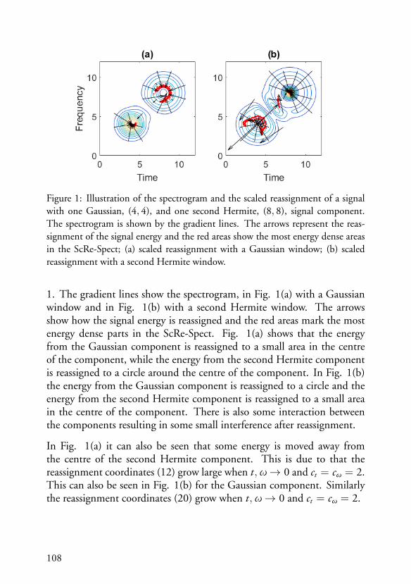
Figure 1: Illustration of the spectrogram and the scaled reassignment of a signalwith one Gaussian, (4, 4), and one second Hermite, (8, 8), signal component.The spectrogram is shown by the gradient lines. The arrows represent the reas-signment of the signal energy and the red areas show the most energy dense areasin the ScRe-Spect; (a) scaled reassignment with a Gaussian window; (b) scaledreassignment with a second Hermite window.

1. The gradient lines show the spectrogram, in Fig. 1(a) with a Gaussianwindow and in Fig. 1(b) with a second Hermite window. The arrowsshow how the signal energy is reassigned and the red areas mark the mostenergy dense parts in the ScRe-Spect. Fig. 1(a) shows that the energyfrom the Gaussian component is reassigned to a small area in the centreof the component, while the energy from the second Hermite componentis reassigned to a circle around the centre of the component. In Fig. 1(b)the energy from the Gaussian component is reassigned to a circle and theenergy from the second Hermite component is reassigned to a small areain the centre of the component. There is also some interaction betweenthe components resulting in some small interference after reassignment.

In Fig. 1(a) it can also be seen that some energy is moved away fromthe centre of the second Hermite component. This is due to that thereassignment coordinates (12) grow large when t,ω→ 0 and ct = cω = 2.This can also be seen in Fig. 1(b) for the Gaussian component. Similarlythe reassignment coordinates (20) grow when t,ω→ 0 and ct = cω = 2.

108

Figure 2: Detection and time-frequency localisation of individual componentsin a multi-component transient signal; (a) the spectrogram with Gaussian win-dow; (b) the spectrogram with second Hermite window; (c) the ScRe-Spect withGaussian window; (d) the ScRe-Spect with second Hermite window.

3 Simulations

A multi-component signal with Gaussian and second Hermite compon-ents can be resolved with the ScRe-Spect using Gaussian and secondHermite time windows. This is illustrated by the simulated signal

x(n) = x1(n− 80)ei2π0.14n + x2(n− 100)ei2π0.18n

+ x3(n− 60)ei2π0.19n + e(n),(21)

where x1(n) and x2(n) are Gaussian functions and x3(n) a second Hermitefunction, all with lengths around 60 samples, and e(n) is white Gaussiannoise, SNR = 15 dB, where SNR is the average total signal energy to thevariance of the noise. Fig. 2 shows the spectrogram and ScRe-Spect. The

109

Figure 3: Two component signal (22), f1 = 0.14, with and without noise, SNR15 dB.

spectrogram and the ScRe-Spect, the illustrations are made in 3D to clearlyshow the difference in amplitude of the peaks, i.e. the energy density. InFig. 2(a), showing the spectrogram with a Gaussian window, only one clearpeak is visible and it is located at (n, f ) = (97, 0.167), however in Fig.2(c), the ScRe-Spect with a Gaussian window, two peaks are clearly seenat (80, 0.140) and (101, 0.180), which are very close to the true centres ofthe two Gaussian components. Fig. 2(b), the spectrogram with a secondHermite window, shows many peaks and is hard to interpret, howeverFig. 2(d) shows only one large peak at (60, 0.190), also present in thecorresponding spectrogram, which is the true centre of the second Hermitecomponent.

3.1 Close components

Detection and localisation of components becomes harder if they are closein time and frequency. For a simulated signal with two components

x(n) = x1(n− 80)ei2πf1n + x2(n− 60)ei2π0.2n + e(n), (22)

where x1(n) is a Gaussian function, x2(n) a second Hermite function ande(n) is white Gaussian noise, SNR 15 dB, we can vary the normalisedfrequency f1 to change the frequency distance between the components.The components overlap in time, see Fig. 3 where f1 = 0.14.

110

Figure 4: The frequency distance between the two components in signal (22)is varied to get the average sample-frequency centres of the largest peaks in theScRe-Spect with Gaussian and second Hermite window respectively, as well as a95% confidence interval, obtained from 200 noise simulations. The true sample-frequency centres of both signal components are also marked; (a) the samplecentres of the largest peaks; (b) the frequency centres of the largest peaks.

We let 0.1 ≤ f1 ≤ 0.19 and simulate 200 signals with different noisefor each f1, to find the average sample-frequency (time-frequency) centresfrom the ScRe-Spect for both signal components. The sample-frequencycentres are obtained by finding the largest peak in the ScRe-Spect, with aGaussian window for the Gaussian component and a second Hermite win-dow for the second Hermite component. The average sample centres andthe 95% confidence intervals are shown in Fig. 4(a). Fig. 4(b) shows theaverage frequency centres and the 95% confidence intervals. It can be seenthat the largest peak in the ScRe-Spect with a matched shape window ac-curately represents the centre of the signal component until the normalisedfrequency distance is only 0.03.

3.2 Noise sensitivity

Detection and localisation of components also becomes harder if the signalhas low SNR. For a sampled signal (22) with f1 = 0.14, the variance of thewhite Gaussian noise e(n) can be varied to evaluate the noise sensitivity of

111

Figure 5: The SNR of the signal (22), f1 = 0.14, is varied to get the averagesample-frequency centres of the largest peaks in the ScRe-Spect with Gaussianand second Hermite window respectively, as well as a 95% confidence interval,obtained from 200 noise simulations. The true sample-frequency centres of bothsignal components are also marked; (a) the sample centre of the largest peaks; (b)the frequency centres of the largest peaks.

the ScRe-Spect. The SNR is varied between 2 and 16 dB and the numberof simulations for each SNR is 200. The average sample centres and 95%confidence intervals from the ScRe-Spect with matching shape window forthe two components are shown in Fig. 5(a). Fig. 5(b) shows the averagefrequency centres and the 95% confidence intervals. It can be seen thatthe method becomes unreliable for the second Hermite component aroundSNR 6 dB, while the localisation of the Gaussian component remains goodeven for low SNR.

4 Transient echolocation signal example

This section provides an example of a transient echolocation signal from abeluga whale (Delphinapterus leucas). The signal is sampled with 1 MHzand recorded by one of 47 simultaneously sampling hydrophones as de-scribed in [15]. The signal was chosen because it is recorded at the centreof the echolocation beam, based on the peak amplitude level the signalis sample by the hydrophone closest to the centre beam axis of the an-

112

Figure 6: Detection and time-frequency localisation of individual components ina dolphin echolocation signal; (a) the spectrogram with Gaussian window; (b)the spectrogram with second Hermite window; (c) the ScRe-Spect with Gaussianwindow; (d) the ScRe-Spect with second Hermite window.

imal. Fig. 6(a) shows the spectrogram with a Gaussian window, Fig. 6(c)the ScRe-Spect with a Gaussian window, Fig. 6(b) the spectrogram witha second Hermite window and Fig. 6(d) the ScRe-Spect with a secondHermite window. Fig. 6(c) shows two peaks, one clear at (307 μs, 65 kHz)and one with smaller amplitude at (338 μs, 53 kHz), these peaks corres-ponds well to the spectrogram in Fig. 6(a). In Fig. 6(d) the signal energy ismore scattered even if peaks appear, the peaks also do not correspond wellto the spectrogram in Fig. 6(b). This suggests that the signal compon-ents in the dolphin echolocation signal more closely resembles Gaussianfunctions than second Hermite functions.

With additional measurements, this method could determine if the largerand smaller Gaussian like components originate from two locations withinthe sound generation mechanism of the dolphin or are the result of internal

113

reflection of the sound wave. Assuming an approximate sound velocity of1490 m/s in the tissue, the time separation of the components correspondsto a total difference in sound wave travel distance of approximately 4.6 cm.

5 Conclusions

It is shown that perfect time-frequency localisation of a Gaussian andsecond Hermite transient signal component can be achieved by the ScRe-Spect using a matching shape time window. If a time window which donot match the shape of the signal component is used, the component en-ergy is instead scattered in ellipses around the time-frequency centre of thecomponent. It is shown that this can be used to find the time-frequencycentres and the shapes of the individual transient signal components withina multi-component signal.

The results from simulated multi-component signals with noise show thatthe ScRe-Spect can resolve and correctly identify the time-frequencycentres and component shapes even if the signal components are closein time and frequency. The ScRe-Spect is also robust to noise disturb-ances. The performance is evaluated on a measured dolphin echolocationsignal, which gives good time-frequency localisation of what seems to betwo Gaussian-like signal components.

114

References

[1] K. Kodera, C. de Villedary, and R. Gendrin, “A new method for thenumerical analysis of nonstationary signals,” Physics of the Earth &Planetary Interiors, vol. 12, pp. 142–150, 1976.

[2] F. Auger and P. Flandrin, “Improving the readability of time-frequency and time-scale representations by the reassignmentmethod,” IEEE Trans. on Signal Processing, vol. 43, pp. 1068–1089,May 1995.

[3] F. Auger, E. Chassande-Mottin, and P. Flandrin, “On phase-magnitude relationships in the short-time Fourier transform,” IEEESignal Processing Letters, vol. 19, no. 5, pp. 267–270, May 2012.

[4] P. Flandrin, “A note on reassigned Gabor spectrograms of Hermitefunctions,” J Fourier Analysis and Applications, vol. 19, no. 2, pp.285–295, 2013.

[5] A.I. Rasiah, R. Togneri, and Y. Attikiouzel, “Modeling 1-D signalsusing Hermite basis functions,” in IEEE Proc.-Vis. Image Signal Pro-cess. IEEE, 1997, vol. 144, pp. 345–354.

[6] T. H. Linh, S. Osowski, and M. Stodolski, “On-line heart beat recog-nition using Hermite polynomials and neuro-fuzzy network,” IEEETrans. on Instrumentation and Measurement, vol. 52, no. 4, pp. 1224–1231, August 2003.

[7] B.N. Li, M.C. Dong, and M.I. Vai, “Modeling cardiovascularphysiological signals using adaptive Hermite and wavelet basis func-tions,” IET Signal Processing, vol. 4, no. 5, pp. 588–597, 2010.

115

[8] R. Ma, Z. Huang L. Shi, and Y. Zhou, “EMP signal reconstruc-tion using associated-Hermite orthogonal functions,” IEEE Trans. onElectromagnetic Compatibility, vol. 64, no. 6, pp. 1383–1390, March2016.

[9] F. Auger, E. Chassande-Mottin, and P. Flandrin, “Making reassign-ment adjustable: The Levenberg-Marquardt approach,” in 2012IEEE International Conference on Acoustics, Speech and Signal Pro-cessing (ICASSP), March 2012, pp. 3889–3892.

[10] M. Hansson-Sandsten and J. Brynolfsson, “The scaled reassignedspectrogram with perfect localization for estimation of Gaussianfunctions,” IEEE Signal Processing Letters, vol. 22, no. 1, pp. 100–104, January 2015.

[11] C. Capus, Y. Pailhas, K. Brown, D.M. Lane, P. Moore, andD. Houser, “Bio-inspired wideband sonar signals based on obser-vations of the bottlenose dolphin (Tursiops truncatus),” J. Acoust.Soc. Am., vol. 121, no. 1, pp. 594–604, 2007.

[12] J. Starkhammar and M. Hansson-Sandsten, “Evaluation of seventime-frequency representation algorithms applied to broadbandecholocation signals,” Advances in Acoustics and Vibration, vol. 2015,pp. 1–13, 2015.

[13] J. Starkhammar, I. Reinhold, P. Moore, D. Houser, and M. Sandsten,“Intra-click time-frequency patterns across the echolocation beam ofa beluga whale,” The Journal of the Acoustical Society of America, vol.140, no. 4, pp. 3239–3239, 2016.

[14] E. Chassande-Mottin, F. Auger, and P. Flandrin, “Reassignment,” inTime-Frequency Analysis, F. Hlawatsch and F. Auger, Eds., chapter 9,pp. 249–277. U.K.: ISTE, London, 2008.

[15] J. Starkhammar, M. Amundin, J. Nilsson, T. Jansson, S. Kuczaj,M. Almqvist, and H.W. Persson, “47-channel burst-mode record-ing hydrophone system enabling measurements of the dynamic echo-location behavior of free-swimming dolphins,” J Acoust Soc Am., vol.126, no. 3, pp. 959–962, 2009.

116