High-Precision Determination of the IsotopicComposition of Dissolved Iron in Iron DepletedSeawater by Double Spike Multicollector-ICPMS

Francois Lacan,*,† Amandine Radic,† Marie Labatut,† Catherine Jeandel,† Franck Poitrasson,‡

Geraldine Sarthou,§ Catherine Pradoux,† Jerome Chmeleff,‡ and Remi Freydier‡,|

LEGOS (CNRS-CNES-IRD-UPS) and LMTG (CNRS-IRD-UPS), Observatoire Midi Pyrenees, 14 av Edouard Belin,31400 Toulouse, France, and LEMAR (CNRS-IRD-UBO), Institut Universitaire Europeen de la Mer,place Nicolas Copernic, 29280 Plouzané, France

This work demonstrates the feasibility of the measurementof the isotopic composition of dissolved iron in seawaterfor an iron concentration range, 0.05-1 nmol L-1, al-lowing measurements in most oceanic waters, includ-ing Fe depleted waters of high nutrient low chlorophyllareas. It presents a detailed description of our previ-ously published protocol, with significant improve-ments on detection limit and blank contribution. Ironis preconcentrated using a nitriloacetic acid superflowresin and purified using an AG 1-×4 anion exchangeresin. The isotopic ratios are measured with a multi-collector-inductively coupled plasma mass spectrom-eter (MC-ICPMS) Neptune, coupled with a desolvator(Aridus II or Apex-Q), using a 57Fe-58Fe double spikemass bias correction. A Monte Carlo test shows thatoptimum precision is obtained for a double spikecomposed of approximately 50% 57Fe and 50% 58Feand a sample to double spike quantity ratio of ap-proximately 1. Total procedural yield is 91 ( 25%(2SD, n ) 55) for sample sizes from 20 to 2 L. Theprocedural blank ranges from 1.4 to 1.1 ng, for samplesizes ranging from 20 to 2 L, respectively, which,converted into Fe concentrations, corresponds to blankcontributions of 0.001 and 0.010 nmol L-1, respec-tively. Measurement precision determined from rep-licate measurements of seawater samples and standardsolutions is 0.08‰ (δ56Fe, 2SD). The precision issufficient to clearly detect and quantify isotopic varia-tions in the oceans, which so far have been observedto span 2.5‰ and thus opens new perspectives toelucidate the oceanic iron cycle.

Iron (Fe) availability has been shown to be the main limitingfactor for phytoplankton growth in wide areas of the world ocean,such as the so-called high nutrient low chlorophyll (HNLC) areas(Southern Ocean, Subarctic, and Equatorial Pacific Ocean).1 In

that respect, the iron oceanic cycle is a component of the globalcarbon cycle and thus of the climate.2 Despite this importance,our knowledge of the iron oceanic cycle remains partial.

Several sources of iron to the open ocean have been proposedand are currently being debated. Whereas dust dissolution wastraditionally considered as the dominant source,3 sediment dis-solution at the continental margins is proposed to significantlycontribute to the Fe content of the open ocean surface waters.4-10

Hydrothermal inputs have recently also been hypothesized assignificant contributors to the Fe content of the open ocean surfacewaters.11 The iron isotopic compositions (Fe IC) of these sourcesappear to be different. In the following, the Fe IC are reported asδ56Fe ) [(56Fe/54Fe)sample/(56Fe/54Fe)IRMM-14 - 1] × 103. Atmo-spheric aerosols have a Fe IC undistinguishable from that ofthe continental crust (δ56Fe ≈ 0.05‰ for the aerosols;12,13 δ56Fe) 0.07 ± 0.02‰, 2SD for the crust14). Pore waters of sedimentsdeposited on shelves and upper slopes display much morenegative Fe IC (-3.4 < δ56Fe < -1.8 for samples just belowthe seawater interface at three sites between 150 and 500 m

* Corresponding author. Fax: +33561253205. E-mail: francois.lacan@legos.obs-mip.fr.

† LEGOS (CNRS-CNES-IRD-UPS), Observatoire Midi Pyrenees.‡ LMTG (CNRS-IRD-UPS), Observatoire Midi Pyrenees.§ LEMAR (CNRS-IRD-UBO), Institut Universitaire Europeen de la Mer.| Current address: HydroSciences Montpellier, Universite Montpellier 2, Place

Eugene Bataillon-34000 Montpellier.

(1) Boyd, P. W.; Jickells, T.; Law, C. S.; Blain, S.; Boyle, E. A.; Buesseler, K. O.;Coale, K. H.; Cullen, J. J.; de Baar, H. J. W.; Follows, M.; Harvey, M.;Lancelot, C.; Levasseur, M.; Owens, N. P. J.; Pollard, R.; Rivkin, R. B.;Sarmiento, J.; Schoemann, V.; Smetacek, V.; Takeda, S.; Tsuda, A.; Turner,S.; Watson, A. J. Science 2007, 315, 612–617.

(2) Martin, J. H. Paleoceanography 1990, 5, 1–13.(3) Jickells, T. D.; An, Z. S.; Andersen, K. K.; Baker, A. R.; Bergametti, G.;

Brooks, N.; Cao, J. J.; Boyd, P. W.; Duce, R. A.; Hunter, K. A.; Kawahata,H.; Kubilay, N.; laRoche, J.; Liss, P. S.; Mahowald, N.; Prospero, J. M.;Ridgwell, A. J.; Tegen, I.; Torres, R. Science 2005, 308, 67–71.

(4) Elrod, V. A.; Berelson, W. M.; Coale, K. H.; Johnson, K. S. Geophys. Res.Lett. 2004, 31, L12307.

(5) Coale, K. H.; Fitzwater, S. E.; Gordon, R. M.; Johnson, K. S.; Barber, R. T.Nature 1996, 379, 621–624.

(6) Blain, S.; Queguiner, B.; Trull, T. Deep-Sea Res., Part II 2008, 55, 559–565.

(7) Moore, J. K.; Braucher, O. Biogeosciences 2008, 5, 631–656.(8) Lam, P. J.; Bishop, J. K. B. Geophys. Res. Lett. 2008, 35, L07608.(9) Tagliabue, A.; Bopp, L.; Aumont, O. Geophys. Res. Lett. 2009, 36, L13601.

(10) Ardelan, M. V.; Holm-Hansen, O.; Hewes, C. D.; Reiss, C. S.; Silva, N. S.;Dulaiova, H.; Steinnes, E.; Sakshaug, E. Biogeosciences , 7, 11–25.

(11) Tagliabue, A.; Bopp, L.; Dutay, J. C.; Bowie, A. R.; Chever, F.; Jean-Baptiste,P.; Bucciarelli, E.; Lannuzel, D.; Remenyi, T.; Sarthou, G.; Aumont, O.;Gehlen, M.; Jeandel, C. Nat. Geosci. 2010, 3, 252–256.

(12) Beard, B. L.; Johnson, C. M. Geochemistry of Non-Traditional Stable Isotopes;Mineralogical Society of America: Washington, DC, 2004; Vol. 55, pp 319-357.

(13) Waeles, M.; Baker, A. R.; Jickells, T.; Hoogewerff, J. Environ. Chem. 2007,4, 233–237.

(14) Poitrasson, F. Chem. Geol. 2006, 235, 195–200.

Anal. Chem. 2010, 82, 7103–7111

10.1021/ac1002504 2010 American Chemical Society 7103Analytical Chemistry, Vol. 82, No. 17, September 1, 2010Published on Web 08/11/2010

depth15,16), while mid-oceanic ridge hydrothermal fluids arecharacterized by δ56Fe ≈ -0.4 (values ranging from δ56Fe )-0.7 to -0.117-19). These distinct isotopic signatures suggest thatiron isotopes could be a very useful tool to better quantify theiron sources to the ocean.17,20

Other uncertainties remain about the Fe internal oceanic cycle,in particular concerning the fluxes between the different Fespecies in the water column, notably the soluble, colloidal, andparticulate phases. Transfers between these phases includenumerous processes, such as dissolution, oxidation followed byprecipitation, photoreduction, sorption, complexation with organicligands, biological uptake, and bacterial remineralization. Noneof these processes has been directly investigated in oceanicconditions regarding Fe isotopic fractionation so far. Howeverseveral in situ and in vitro studies in other media (e.g., fresh water)have been realized (dissolution,13,21 oxidation followed byprecipitation,12,22 sorption,23,24 siderophore complexation,25 anduptake by plants26). Some of these processes and associated Feisotopic fractionations may complicate the use of Fe isotopes asa tracer of iron sources in the open ocean. On the other hand,they may provide new insights into the internal oceanic Fe cycle,such as iron speciation, dissolved/particulate fluxes, or biologicalprocesses. In such a context, multiparametric and multi-isotopicapproaches and a better description of laboratory determinedisotopic fractionation factors in realistic open oceanic conditionsmay be useful.

This great potential motivated very numerous Fe isotopestudies during the past decade in the marine environment and atthe ocean boundaries (ferromanganese crusts, plankton tows,aerosols, sediments, pore waters, suspended particles, rivers,estuaries, hydrothermal vents20,27-30). However, because of theanalytical difficulty of such measurement, the only data of theisotopic composition of the iron dissolved in seawater in the openocean published so far to our knowledge are those obtained with

the protocol described here.31 Ranges of values have beenreported in the San Pedro Basin (δ56Fe ) -1.82 to 0‰) and inthe Western Subtropical North Atlantic (δ56Fe ) +0.3 to+0.7‰).37 Finally, the samples used in the present study havedissolved Fe (DFe) IC in the following ranges, δ56Fe ) -0.13to +0.27 in the South East Atlantic (Cape Basin), δ56Fe )-0.49to -0.19 in the Atlantic sector of the Southern Ocean Antarcticzone, δ56Fe ) +0.22 to +0.40 in the Western and CentralEquatorial Pacific, and δ56Fe ) +0.41 to +0.52 in the WesternSubtropical North Atlantic. Documenting the IC of DFe isextremely important because dissolved iron in seawater is thephase which links all the above listed marine phases. It is, forinstance, necessary to exploit phytoplankton or ferromanganeseFe IC. Before being able to measure the Fe IC of the differentFe forms included in the operationally defined “dissolved” form(e.g., colloids, nanoparticles, and free ionic Fe), the measure-ment of the dissolved pool is a major step forward.

DFe concentration in open ocean depleted surface waters canbe as low as ∼0.02 nmol L-1 (nM),32 and reach a typical valueof 0.6 nM at depth.7 The minimum amount of iron required toperform a precise isotopic analysis (i.e., typical precision <0.1‰2SD) is around 20 ng (refs 33 and 34 and this work). Therefore,analyzing the DFe IC in Fe depleted seawater requires thepreconcentration of ∼20 L samples (20 L of seawater with [Fe] )0.02 nmol L-1 contain 22 ng of Fe). Twelve years ago, a Fepreconcentration method based on Mg(OH)2 precipitation waspublished.35 This method appeared promising for the analysisof the Fe IC because of its low blank level. However, it producesrather voluminous precipitates, which are difficult to handle.De Jong et al.29 managed to measure the DFe IC of seawaterin the North Sea using such coprecipitation. However thismethod was restricted to samples smaller than 2 L, with aprocedural blank of ∼10 ng, which, converted into Fe concen-tration, corresponds to a blank contribution of 0.9 nM (10 ngin 2 L). It was therefore unsuitable for open ocean Feconcentrations. We also tested this method at LEGOS but gaveup because of the volume of the precipitate that was excessivelylarge for further chromatographic purification. Then, adaptinga protocol for the preconcentration of 2 mL seawater samplesfor the determination of its DFe concentration,36 we developeda protocol for the analysis of the DFe IC, using a commerciallyavailable nitriloacetic acid (NTA) superflow resin (Qiagen),packed in a column, that allowed the measurement of 10 Lsamples with a blank of 8 ng.31 This blank contribution, of 0.014nM, allowed measuring samples with [DFe] > 0.14 nM (i.e.,blank contribution <10%) but was unsuitable for HNLC areasurface waters, which concentrations are often around 0.05 nM.The use of the same resin in a bulk extraction technique wasthen reported on 1 L samples, with a blank of 1.1 ng.37 Although

(15) Severmann, S.; Johnson, C. M.; Beard, B. L.; McManus, J. Geochim.Cosmochim. Acta 2006, 70, 2006–2022.

(16) Homoky, W. B.; Severmann, S.; Mills, R. A.; Statham, P. J.; Fones, G. R.Geology 2009, 37, 751–754.

(17) Beard, B. L.; Johnson, C. M.; Von Damm, K. L.; Poulson, R. L. Geology2003, 31, 629–632.

(18) Sharma, M.; Polizzotto, M.; Anbar, A. D. Earth Planet. Sci. Lett. 2001,194, 39–51.

(19) Rouxel, O.; Shanks, W. C.; Bach, W.; Edwards, K. J. Chem. Geol. 2008,252, 214–227.

(20) Zhu, X.-K.; O’Nions, R. K.; Guo, Y.; Reynolds, B. C. Science 2000, 287,2000–2002.

(21) Wiederhold, J. G.; Kraemer, S. M.; Teutsch, N.; Borer, P. M.; Halliday,A. N.; Kretzschmar, R. Environ. Sci. Technol. 2006, 40, 3787–3793.

(22) Bullen, T. D.; White, A. F.; Childs, C. W.; Vivit, D. V.; Schulz, M. S. Geology2001, 29, 699–702.

(23) Crosby, H. A.; Roden, E. E.; Johnson, C. M.; Beard, B. L. Geobiology 2007,5, 169–189.

(24) Johnson, C. M.; Beard, B. L.; Roden, E. E. Annu. Rev. Earth.Planet. Sci.2008, 36, 457–493.

(25) Dideriksen, K.; Baker, J. A.; Stipp, S. L. S. Earth Planet. Sci. Lett. 2008,269, 280–290.

(26) Guelke, M.; Von Blanckenburg, F. Environ. Sci. Technol. 2007, 41, 1896–1901.

(27) Rouxel, O.; Dobbek, N.; Ludden, J.; Fouquet, Y. Chem. Geol. 2003, 202,155–182.

(28) Bergquist, B. A.; Boyle, E. A. Earth Planet. Sci. Lett. 2006, 248, 54–68.(29) de Jong, J.; Schoemann, V.; Tison, J. L.; Becquevort, S.; Masson, F.;

Lannuzel, D.; Petit, J.; Chou, L.; Weis, D.; Mattielli, N. Anal. Chim. Acta2007, 589, 105–119.

(30) Levasseur, S.; Frank, M.; Hein, J. R.; Halliday, A. Earth Planet. Sci. Lett.2004, 224, 91–105.

(31) Lacan, F.; Radic, A.; Jeandel, C.; Poitrasson, F.; Sarthou, G.; Pradoux, C.;Freydier, R. Geophys. Res. Lett. 2008, 35, L24610.

(32) Sarthou, G.; Baker, A. R.; Blain, S.; Achterberg, E. P.; Boye, M.; Bowie,A. R.; Croot, P.; Laan, P.; de Baar, H. J. W.; Jickells, T. D.; Worsfold, P. J.Deep-Sea Res., Part I 2003, 50, 1339–1352.

(33) Weyer, S.; Schwieters, J. B. Int. J. Mass Spectrom. 2003, 226, 355–368.(34) Schoenberg, R.; von Blanckenburg, F. Int. J. Mass Spectrom. 2005, 242,

257–272.(35) Wu, J.; Boyle, E. A. Anal. Chim. Acta 1998, 367, 183–191.(36) Lohan, M. C.; Aguilar-Islas, A. M.; Franks, R. P.; Bruland, K. W. Anal. Chim.

Acta 2005, 530, 121–129.(37) John, S. G.; Adkins, J. F. Mar. Chem. 2010, 119, 65–76.

7104 Analytical Chemistry, Vol. 82, No. 17, September 1, 2010

the use of a smaller volume facilitates sampling and handlingissues and although the absolute value of that blank wassignificantly reduced compared to previous studies, whenscaled to the sample volume, the blank contribution of thattechnique, 0.020 nM (1.1 ng in 1 L), was slightly larger thanthat of Lacan et al. (2008).31

In this paper, we present a detailed description of the protocolbriefly presented in Lacan et al.,31 with significant improvementson detection limit and blank contribution. This protocol allowsthe measurement of the isotopic composition of dissolved iron inseawater, for Fe concentrations down to 0.05 nM (blank contribu-tion of 0.001 nM).

EXPERIMENTAL SECTIONSampling. Seawater samples of 10-20 L were collected with

acid-cleaned 12 L Go-Flo bottles mounted on a trace metal cleanrosette or directly on a Kevlar wire. The Go-Flo bottles werebrought into a trace metal clean container for filtration through0.45 µm Nuclepore membranes (90 mm), within a few hours ofcollection. Filtration was performed from the Go-Flo bottles(pressurized with 0.02 µm filtered nitrogen), through PFA filtrationunits (Savillex), directly into a 20 L flexible LDPE container (withPP closure; Fillaud). Samples were then acidified onboard (1.7mL L-1 of seawater of 9 M HCl, twice distilled in a Picotracesub-boiling distillation system) and stored double bagged.

Chemical Separation General Points. All of the chemicalseparation procedure was conducted in a trace metal clean lab,equipped with an ISO 4 (class 10) laminar flow hood. High-purityreagents were used (either twice distilled at LEGOS or com-mercially available). All labware was acid cleaned. Blanks ofreagents, labware, and atmosphere were monitored.

Fe IC measurement in seawater requires the Fe extractionfrom the sample matrix with (i) a high yield (because of its lowabundance), (ii) low contamination levels, (iii) no isotopic frac-tionation or a method for correcting for it, and (iv) a sufficientseparation of the elements interfering with Fe isotopes during thespectrometric analysis.

Most of the tests described below were performed on 10 Lsamples, but the method has also been validated for samplevolumes ranging from 2 to 20 L.

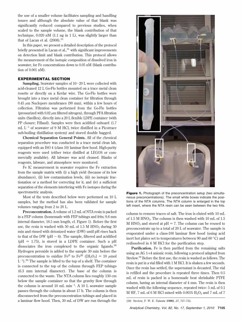
Preconcentration. A volume of 1.2 mL of NTA resin is packedin a FEP column (homemade with FEP tubings and frits; 9.6 mminternal diameter, 16.5 mm length, cf. Figure 1). Before the firstuse, the resin is washed with 50 mL of 1.5 M HNO3 during 30min and rinsed with deionized water (DW) until pH rises backto that of the DW (pH ∼ 6). The sample, filtered and acidified(pH ) 1.75), is stored in a LDPE container. Such a pHdissociates the iron complexed to the organic ligands.36

Hydrogen peroxide is added to the sample 30 min before thepreconcentration to oxidize FeII to FeIII ([H2O2] ) 10 µmolL-1).36 The sample is lifted to the top of a shelf. The containeris connected to the top of the column through FEP tubings(6.3 mm internal diameter). The base of the column isconnected to the waste. The NTA column lies roughly 130 cmbelow the sample container so that the gravity flow throughthe column is around 10 mL min-1. A 10 L seawater samplepasses through the column in about 17 h. The column is thendisconnected from the preconcentration tubings and placed ina laminar flow hood. Then, 30 mL of DW are run through the

column to remove traces of salt. The iron is eluted with 10 mLof 1.5 M HNO3. The column is then washed with 10 mL of 1.5M HNO3 and stored at pH ) 7. The column can be reused topreconcentrate up to a total of 20 L of seawater. The sample isevaporated under a class-100 laminar flow hood (using acidinert hot plates set to temperatures between 90 and 60 °C) andredissolved in 6 M HCl for the purification step.

Purification. Fe is then purified from the remaining saltsusing an AG 1-×4 anionic resin, following a protocol adapted fromStrelow.38 Before the first use, the resin is washed as follows. Theresin is put in a vial filled with 1 M HCl. It is shaken a few seconds.Once the resin has settled, the supernatant is decanted. The vialis refilled and the procedure is repeated three times. Then 0.5mL of resin is packed in a homemade heat shrinkable PTFEcolumn, having an internal diameter of 4 mm. The resin is thenwashed with the following sequence, repeated twice: 5 mL of 0.1M HF, 7 mL of 6 M HCl mixed with 0.001% H2O2 and 7 mL of 7

(38) Strelow, F. W. E. Talanta 1980, 27, 727–732.

Figure 1. Photograph of the preconcentration setup (two simulta-neous preconcentrations). The small white boxes indicate the posi-tions of the NTA columns. The NTA column is enlarged in the topleft insert, where the NTA resin can be seen between the two frits.

7105Analytical Chemistry, Vol. 82, No. 17, September 1, 2010

M HNO3. It is stored in 0.01 M HCl. The column is ready foruse. Before loading the sample, the resin is conditioned twicewith 0.5 mL of 6 M HCl mixed with 0.001% H2O2. The sampleis loaded onto the resin in 0.5 mL of 6 M HCl mixed with 0.001%H2O2. Most of the elements are first eluted with 3.5 mL of 6 MHCl mixed with 0.001% H2O2. Iron is then eluted with 3 mL of1 M HCl mixed with 0.001% H2O2. The elements remaining inthe resin are washed with 5 mL of 0.1 M HF, then 7 mL of 6M HCl mixed with 0.001% H2O2 and 7 mL of 7 M HNO3. Theresin is stored in 0.01 M HCl. The use of H2O2 notably avoidsthe elution of Mo within the Fe fraction.

Isotopic Analysis. A multicollector-inductively coupled plasmamass spectrometer (MC-ICPMS) Neptune (Thermo Scientific) isused, coupled with a desolvating nebulizer system, either aCETAC Aridus II or an ESI Apex-Q without a membrane.Measurements are performed using medium or high resolutionslits in order to resolve polyatomic interferences on masses 54,56, and 57 (e.g., 40Ar14N, 40Ar16O, 40Ca16O, 40Ar16O1H).33 “X”skimmer cones are also used to enhance the sensitivity. Thevery low Fe content of the samples imposes the use of suchdevices. The operation parameters are reported in Table 1 andthe collector configuration in Table 2. This setting allows measur-ing all stable Fe isotopes as well as monitoring Cr and Ni, whichcan produce isobaric interferences with Fe.

The spectrometer mass fractionation (mass bias) is correctedwith a 57Fe-58Fe double spike. This method has advantagescompared to the standard bracketing method or to an inter-element normalization (using Ni or Cr) because it allowsmeasuring the mass bias (i) during the sample measurement(which is not the case of the standard bracketing method) and(ii) using the same element as that measured (which is notthe case of the interelement normalization). In addition, the

double spike method allows correcting for potential isotopefractionation during chemical separation, provided that thefractionation law is the same during chemical separation andwithin the spectrometer.39 This assumption is currently made.40,41

The use of a double spike also allows the determination of the Feconcentration using the isotopic dilution method.

The isotopes 57Fe and 58Fe are chosen for the double spikebecause they have the two lowest natural abundances amongthe Fe isotopes. This allows optimizing the beam intensitiesof all Fe isotopes, which is critical for samples with very lowFe content. Data reduction is performed using the iterativeapproach of Siebert et al.40 Assuming that the natural andartificial (during chemical separation and within the spectrom-eter) fractionations are mass dependent, a single analysis ofthe sample-double spike mixture is sufficient to determinethe true sample Fe IC.

The 57Fe-58Fe double spike is prepared from two mono-isotope solutions (a 57Fe solution with the following abundancesA54Fe ) 0.18%, A56Fe ) 5.33%, A57Fe ) 92.57%, and A58Fe )1.92% and a 58Fe solution with the following abundances A54Fe) 0.004%, A56Fe ) 0.07%, A57Fe ) 8.22%, and A58Fe ) 91.71%).The isotopic composition of the double spike and the doublespike to sample mixing ratio are optimized to minimize errorpropagation during data reduction.

The double spike is added to the acidified sample at least 12 hbefore the preconcentration to allow the homogenization of thedouble spike with the sample. A preliminary determination or anestimation of the sample Fe concentration is therefore necessary.After preconcentration and purification, the sample is dissolvedin ∼0.7 mL of 0.3 M HNO3 for the spectrometric analysis. Theexact volume is determined depending on the spectrometeruptake flow rate (varying between ∼50 and 120 µL min-1, cf.Table 1), in order to maximize beam intensities.

Each measurement session begins with repeated measure-ments of the ETH (Eidgenossische Technische HochschuleZurich) in-house hematite standard42 (named ETH-STD hereafter;mixed with the double spike), relative to IRMM 14 (mixed withthe double spike). The ETH-STD (mixed with the double spike)is then run every 80 min in order to monitor accuracy andprecision of the instrument. Each measurement is bracketed withan instrumental blank (0.3 M HNO3 used to dissolve thestandards and samples). Acquisition times are set to 25 cycles

(39) Russel, W. A.; Papanastassiou, D. A.; Tombrello, T. A. Geochim. Cosmochim.Acta 1978, 42, 1075–1090.

(40) Siebert, C.; Nagler, T. F.; Kraners, J. D. Geochem. Geophys. Geosyst. 2001,2, 1032, DOI: 10.1029/2000GC000124.

(41) Dideriksen, K.; Baker, J. A.; Stipp, S. L. S. Geochim. Cosmochim. Acta 2006,70, 118–132.

(42) Poitrasson, F.; Freydier, R. Chem. Geol. 2005, 222, 132–147.

Table 1. Operation Parameters of the ThermoFinniganNeptune MC-ICPMS at the Observatoire Midi Pyrenees

Standard Conditions for Fe Analysisrf power 1200 Wacceleration voltage 10 kVmass analyzer pressure 1.0 × 10-8 mbarextraction lens -2000 V

Desolvating Sample Introduction Systems

Cetac Aridusspray chamber ESI PFA Teflon upgradespray chamber temperature 110 °Cdesolvating membrane

temperature160 °C

argon sweep gas flow ∼6.5 L min-1

nitrogen additional gas ∼10 mL min-1

nebulizer ESI MicroFlow PFA 100sample uptake rate ∼120 µL min-1

transmission efficiency 0.020% (30 µm slit, m/∆m ≈ 9000)0.009% (16 µm slit, m/∆m ≈ 13 500)

mass discrimination 2.8% per amu

ESI Apex-Qheater temperature 100 °Cchiller temperature 2 °Cnitrogen gas flow 0nebulizer ESI MicroFlow PFA 75sample uptake rate 60-80 µLmin-1

transmission efficiency 0.028% (50 µm slit, m/∆m ≈ 7400)0.018% (18 µm slit, m/∆m ≈ 13 000)

mass discrimination 2.4% per amu

Table 2. Faraday Cup Configuration and IsotopicAbundances of Fe and Elements That Can ProduceIsobaric Interferences with Fe

nominal mass 53 54 56 57 58 60 61

isotope abundance (%) Cr 9.5 2.37Fe 5.8 91.7 2.2 0.28Ni 68.3 26.1 1.13

collector configuration L4 L2 L1 H1 H2 H3 H4

7106 Analytical Chemistry, Vol. 82, No. 17, September 1, 2010

of 8.4 s for samples (and standards) and 10 cycles of 8.4 s forblanks. Uptake time is set to the minimum, here 55 s, in orderto save as much sample as possible for the acquisition. Washtime is set to the minimum (20 s) for the samples (becausethey follow blanks), whereas it is set to 150 s for blanks inorder to wash traces of Fe remaining from the previous sample(or standard). The absence of memory effect after such a washis monitored between each sample (or standard) by checkingthat the 10 cycles of each blank do not display a decreasingtrend. The average beam intensities of the bracketing instru-mental blanks are subtracted to those of the sample. Cr andNi interferences are also subtracted to the sample beamintensities. 54Cr and 58Ni interferences are estimated from the53Cr and 60Ni beams, taking into account the instrumental massfractionation for Fe, determined by the double spike massfractionation correction. Instrumental blanks and interferencesare most of the time lower than 0.1% (with maximum valuesreaching 0.5%). The Fe IC is finally corrected for the blank ofthe overall procedure, which Fe IC is taken to be that of theigneous rocks.43

RESULTS AND DISCUSSIONIsotopic Analysis Optimization. Two desolvators, the Aridus

II and the Apex-Q (without membrane) were used. Instrumentalisotopic fractionation was found much more stable with the Apex-Q(typical mass bias variations of 0.05% over 10 h) than with theAridus II (mass bias variation up to 1% over 10 h). The Apex-Qand Aridus II provided sensitivities ∼5 and 3 times higher thanthe stable introduction system (SIS, Elemental Scientific Inc.),respectively (taking into account sample uptake rates). The ApexQ (without membrane) is therefore now preferred because of itsmore stable mass fractionation and higher sensitivity relative tothe Aridus II.

The widths of the medium and high resolution (MR and HR)slits were changed by Thermo Scientific in 2008, from 30 and 16µm to 50 and 18 µm, respectively. Until 2008, an unused MR slit(30 µm) and a HR slit (16 µm) lead to typical mass resolution(m/∆m of the peak side 5% to 95% peak height, measured on 56Fe)of 9000 and 13 000, respectively, which allowed resolvingpolyatomic interferences. This is now extremely difficult withthe new MR slit width (50 µm), leading to typical resolutionsof 7400. The HR slit (18 µm) is thus now almost alwayspreferred, although it reduces the transmission. A 30 µm widthslit would provide better performance but is no more com-mercially available today.

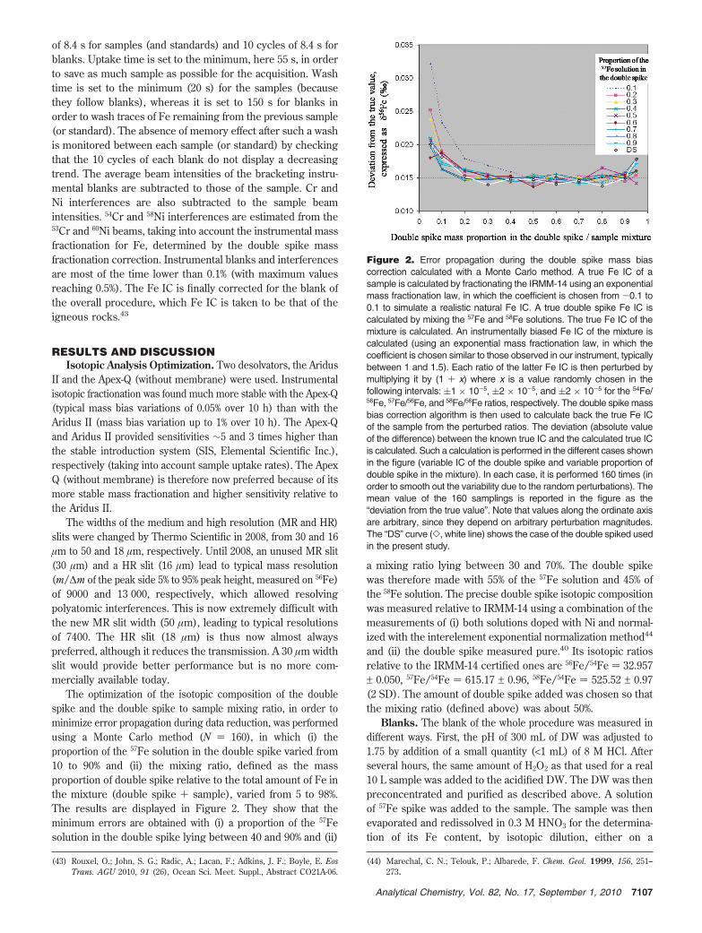
The optimization of the isotopic composition of the doublespike and the double spike to sample mixing ratio, in order tominimize error propagation during data reduction, was performedusing a Monte Carlo method (N ) 160), in which (i) theproportion of the 57Fe solution in the double spike varied from10 to 90% and (ii) the mixing ratio, defined as the massproportion of double spike relative to the total amount of Fe inthe mixture (double spike + sample), varied from 5 to 98%.The results are displayed in Figure 2. They show that theminimum errors are obtained with (i) a proportion of the 57Fesolution in the double spike lying between 40 and 90% and (ii)

a mixing ratio lying between 30 and 70%. The double spikewas therefore made with 55% of the 57Fe solution and 45% ofthe 58Fe solution. The precise double spike isotopic compositionwas measured relative to IRMM-14 using a combination of themeasurements of (i) both solutions doped with Ni and normal-ized with the interelement exponential normalization method44

and (ii) the double spike measured pure.40 Its isotopic ratiosrelative to the IRMM-14 certified ones are 56Fe/54Fe ) 32.957± 0.050, 57Fe/54Fe ) 615.17 ± 0.96, 58Fe/54Fe ) 525.52 ± 0.97(2 SD). The amount of double spike added was chosen so thatthe mixing ratio (defined above) was about 50%.

Blanks. The blank of the whole procedure was measured indifferent ways. First, the pH of 300 mL of DW was adjusted to1.75 by addition of a small quantity (<1 mL) of 8 M HCl. Afterseveral hours, the same amount of H2O2 as that used for a real10 L sample was added to the acidified DW. The DW was thenpreconcentrated and purified as described above. A solutionof 57Fe spike was added to the sample. The sample was thenevaporated and redissolved in 0.3 M HNO3 for the determina-tion of its Fe content, by isotopic dilution, either on a

(43) Rouxel, O.; John, S. G.; Radic, A.; Lacan, F.; Adkins, J. F.; Boyle, E. EosTrans. AGU 2010, 91 (26), Ocean Sci. Meet. Suppl., Abstract CO21A-06.

(44) Marechal, C. N.; Telouk, P.; Albarede, F. Chem. Geol. 1999, 156, 251–273.

Figure 2. Error propagation during the double spike mass biascorrection calculated with a Monte Carlo method. A true Fe IC of asample is calculated by fractionating the IRMM-14 using an exponentialmass fractionation law, in which the coefficient is chosen from -0.1 to0.1 to simulate a realistic natural Fe IC. A true double spike Fe IC iscalculated by mixing the 57Fe and 58Fe solutions. The true Fe IC of themixture is calculated. An instrumentally biased Fe IC of the mixture iscalculated (using an exponential mass fractionation law, in which thecoefficient is chosen similar to those observed in our instrument, typicallybetween 1 and 1.5). Each ratio of the latter Fe IC is then perturbed bymultiplying it by (1 + x) where x is a value randomly chosen in thefollowing intervals: (1 × 10-5, (2 × 10-5, and (2 × 10-5 for the 54Fe/56Fe, 57Fe/56Fe, and 58Fe/56Fe ratios, respectively. The double spike massbias correction algorithm is then used to calculate back the true Fe ICof the sample from the perturbed ratios. The deviation (absolute valueof the difference) between the known true IC and the calculated true ICis calculated. Such a calculation is performed in the different cases shownin the figure (variable IC of the double spike and variable proportion ofdouble spike in the mixture). In each case, it is performed 160 times (inorder to smooth out the variability due to the random perturbations). Themean value of the 160 samplings is reported in the figure as the“deviation from the true value”. Note that values along the ordinate axisare arbitrary, since they depend on arbitrary perturbation magnitudes.The “DS” curve (], white line) shows the case of the double spiked usedin the present study.

7107Analytical Chemistry, Vol. 82, No. 17, September 1, 2010

quadrupole ICPMS (Agilent 7500, with a collision cell in Hemode) or on the MC-ICPMS (mass fractionation corrected forby standard bracketing). This blank (preconcentration +purification) was initially 8.0 ng when the method was firstdeveloped,31 then progressively reduced to 2.9 ± 1.6 ng (2SD,n ) 8), and is now 1.04 ± 0.6 ng (2SD, n ) 6). This verysignificant improvement is the result of the progressivereplacement of HDPE and LDPE labware by Teflon labware(FEP, PTFE, and PFA) and increased care in handling. Theblank of each step of the protocol were also measuredindividually: NTA preconcentration and AG 1-×4 purificationblanks are found to amount to 0.40 ± 0.25 and 0.64 ± 0.35ng (2SD, n ) 6), respectively. The H2O2 blank is negligible(∼1 pg).

For a real seawater sample, the blank from the sampleacidification needs to be considered (more acid is used than for300 mL of DW). The acid used here was obtained at LEGOS bytwo consecutive distillations (Picotrace sub-boiling distillationsystem). Its Fe concentration was 10 × 10-12 g g-1 (i.e., 0.18 nmolL-1) for a HCl concentration of 9 M (this is similar to thecleanest commercially available HCl to our knowledge). Theacid quantity (for such a molarity) required to lower the sea-water pH to 1.75 is 1.7 mL/L of seawater. This leads to anacidification blank corresponding to 0.3 pM, i.e., about 1.5% ofthe natural iron in the most depleted waters (0.02 nM). Acidpurity has to be carefully monitored since much higher blanksmay be found in some HCl solutions, even twice distilled.

Filtration and storage blanks also have to be considered. Theyare however difficult to estimate. For that purpose, we comparedthe Fe concentrations determined with the present protocol withthose obtained independently from duplicate samples (samelocation but successive casts) with well established techniques,using a different filtration (e.g., Sartobran capsules), differentcontainers (e.g., 60 mL bottles), and flow injection analysis.32 Theformer concentrations were found lower than or equal to the latter.This implies that filtration and storage blanks of the presentprotocol are negligible or at least as good as those of the wellestablished techniques. Moreover this validates the entire protocol(including sampling, filtration, acidification, storage, preconcen-tration, purification, and spectrometric analysis) regarding blankissues. This was tested for sample sizes up to 20 L and Feconcentrations down to 0.05 nM (compared to 10 L and 0.1 nMin Lacan et al.31).

In total, the procedural blank is therefore the sum of (i) 1.04ng coming from the preconcentration and purification steps and(ii) the acidification blank that depends on sample size. It rangesfrom 1.4 to 1.1 ng, for sample sizes ranging from 20 to 2 L,respectively, which converted into Fe concentrations, correspondsto total blank contributions of 0.001 and 0.010 nmol L-1,respectively.

The isotopic composition of the total procedural blank isunknown (in particular that coming from the acidification). Ourattempts to measure it were unfruitful because of the too low Fequantities. However NTA blanks have been reported with δ56Feranging from -0.5 and +0.5‰, converging toward igneous rockFe IC as the blank increased.43 In order to correct for theprocedural blank contribution to the measured ratios, it wastherefore assumed that it is characterized by the IC of igneous

rocks. The implication of a deviation from that value can beestimated. It depends on the Fe content of the sample. Forinstance, for a 10 L sample with a Fe concentration of 0.05 nM,i.e., 56 ng of Fe, if the blank Fe IC deviates from the assumedvalue by less than 3.7‰, then the blank correction would implya bias lower than 0.08‰ (the measurement precision, cf. below)on the final result.

Yields. The total yield of the chemical Fe preconcentrationand purification was determined as follows. A 10 L seawatersample, taken at ∼40 m depth at the Dyfamed site (NorthwestMediterranean), was filtered (SUPOR 47 mm, 0.8 µm), thenacidified, and spiked with a solution of 57Fe (for the determinationof its Fe concentration by isotopic dilution). The sample wasthen taken through the entire procedure. The resulting Fe wasmeasured on the quadrupole ICPMS, both by the isotopicdilution method and the external calibration method (combinedwith a sensitivity correction with indium as an internalstandard). After correction for the blank contribution, theisotopic dilution method allowed determining the initial con-centration of the sample and the external standard methodallowed determining the Fe quantity recovered after thepurification. Comparison of both quantities allowed calculatingthe total yield of the procedure. This has been measuredrepeatedly at each chemistry session. The total Fe yield is 92± 25% (2SD, n ) 55). This value confirms, with much moredata, what was previously established in Lacan et al.,31 whoreported 92 ± 20% (2SD, n ) 5). Note that achieving a 100%yield is not necessary since a double spike is added before thechemical procedure. The preconcentration and purification stepyields were also measured separately, with similar techniques.The purification step is quantitative (100% yield for Fe), whereasthe preconcentration step yield is 92%. Where the method wastested for samples volumes up to 10 L only in Lacan et al.,31

we also performed yield measurements on 20 L samples in thepresent study, which are found to be 98 ± 9% (2SD, n ) 2).

General Performances of the AG 1-×4 Column. In orderto better understand the behavior of the AG 1-×4 resin, it wastested using multielemental standard solutions (quantities around10-100 ng for most elements, up to a few micrograms for majorelements such as Si or Ca). The multielemental standard wasevaporated, redissolved in 0.5 mL of 6 M HCl mixed with 0.001%H2O2, and loaded onto the resin. The concentrations of thedifferent elements in the successive elution solutions weremeasured with the Agilent 7500 ICPMS. Table 3 displays theyields for the different elements. The test was replicated six times.The results were always the same (within instrument precision,typically of 2%), which shows the robustness of this protocol. Thistest shows that the column is very efficient at separating most ofthe elements from the Fe fraction, notably major ions such asNa, Mg, or Ca. Only U and Ga are quantitatively eluted togetherwith Fe and to a lower extent Sb and In, which are partially elutedtogether with Fe.

Matrix. The performance of the chemical separation was alsoassessed by the measurement of the matrix in which the Fe iseluted. This was determined similarly to the yield determinations.A 10 L Dyfamed seawater sample was first preconcentrated withthe NTA column. The elemental composition of the preconcen-trated sample was then measured on the quadrupole ICPMS. Most

7108 Analytical Chemistry, Vol. 82, No. 17, September 1, 2010

of the elements (those measurable with the ICPMS technique)were measured. The amount of solid residue eluted with the Feweighs only about 70 µg. Therefore, 99.999 98% of the total dissolvedsolids of the initial 10 L seawater sample (350 g) are rejected. Mostof the residue (>90%) is composed of Mg, Na, and Ca. It also containstraces of V, Mo, Sb, K, Sr, Cu, Ti, Ga, Sn, B, U, and Al.

The same measurements were performed after the purificationstep.31 At this stage, the elements eluted together with Fe aremostly Ca, Ga, and Sb (∼ 90, 30, and 20 ng, respectively). Thereare also traces of U, B, and Mg. In total, the matrix solid residueweighs ∼150 ng. No traces of Cr, Ni, or Zn could be detectedwithin the Fe fraction. The separation of Ni and Cr was found asefficient for 20 L samples as for 10 L samples (other elementsnot measured). The concentrations of matrix ions in the finalsolution for MC-ICPMS are a function of the volume used todissolve the sample. For a typical volume of 600 µL, the abovequantities yield to 150, 50, and 33 ppb, for Ca, Ga, and Sb,respectively. These results differ from what is obtained from amultielemental standard solution (Table 3) because they reflectthe initial matrix of seawater, which some of the major elements(e.g., Mg and Ca) are still present in the Fe fraction even if theyare found at undetectable levels in the tests performed withstandard solutions.

Precision and Accuracy. The three ratios δ56Fe, δ57Fe, andδ58Fe are measured with the same accuracy and the sameinternal and external precisions per atomic mass unit. Internalprecision of the measurements is typically 0.06‰ (δ56Fe; 2SE) 2SD/�n, where SE and SD stand for standard error andstandard deviation, respectively). This value is lower than theexternal precisions reported below. Except rare instances inwhich internal precision is larger than external precision,external precision, rather than internal precision, determinesthe measurement precision and is described below.

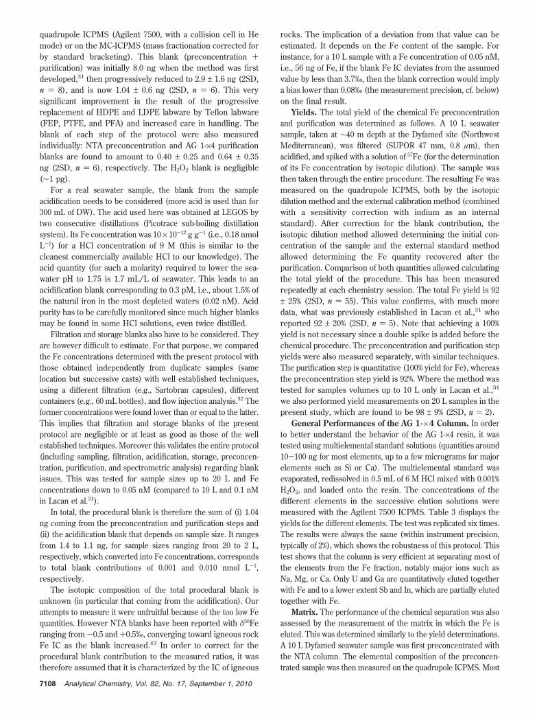
Precision and accuracy of the Fe IC measurement were testedin different ways. First, the measurement of variable amounts ofthe ETH-STD (relative to IRMM-14) allowed estimating thecapabilities of our instrument, configuration, and data reductionfor variable Fe consumptions. These results are reported in Figure3. The Fe IC of the ETH-STD has been measured in severallaboratories with different instruments. Its mean value from thedata obtained in the different laboratories is δ56Fe(ETH-STD) )

0.53 ± 0.06‰ (2SD, n ) 6).30,41,42,45-47 Taking into account thewhole of our measurements, which correspond to Fe consump-tions ranging from 165 to 20 ng per analysis, we found δ56Fe(ETH-STD) ) 0.52 ± 0.08‰ (2SD, n ) 81, over a period of 1 year).Narrowing this scale, for the measurements with low Fecontents, with Fe consumption ranging from 40 to 20 ng, wefound δ56Fe(ETH-STD) ) 0.52 ± 0.10‰ (2SD, n ) 10). Theseresults are in very good agreement with what we obtainedpreviously δ56Fe(ETH-STD) ) 0.53 ± 0.09‰ (2SD, n ) 40, for200 to 25 ng, over a period of 4 months)31 and with the valuesmeasured in the other laboratories. It can therefore beconcluded that the present measurements are unbiased.

Accuracy of the spectrometric analysis was also tested byrealizing a blind test. The isotopic composition of two ironsolutions (solid samples digested and purified with the AG 1-×4resin) were measured by one of the authors following Poitrassonand Freydier42 (Ni mass bias correction, ESI stable introductionsystem, typical [Fe] of the analyzed solution of 3 ppm). Thesolutions were then measured using the present protocol byanother author to whom the preceding results were not com-municated. The results, displayed in Figure 4, show that theresults obtained by both techniques are identical within measure-ment uncertainties.

(45) Williams, H. M.; Markowski, A.; Quitte, G.; Halliday, A. N.; Teutsch, N.;Levasseur, S. Earth Planet. Sci. Lett. 2006, 250, 486–500.

(46) Fehr, M. A.; Andersson, P. S.; Halenius, U.; Morth, C. M. Geochim.Cosmochim. Acta 2008, 72, 807–826.

(47) Teutsch, N.; von Gunten, U.; Porcelli, D.; Cirpka, O. A.; Halliday, A. N.Geochim. Cosmochim. Acta 2005, 69, 4175–4185.

Table 3. Yields (%) of the AG 1-×4 Column, For Different Elements in the Successive Elution Solutions

3.5 mL of 6 M HCl+ 0.001% H2O2

3 mL of 1 M HCl+ 0.001% H2O2

3 mL of0.1 M HF

7 mL of 6 M HCl+ 0.001% H2O2

7 mL of7 M HNO3 total

Li, B, Na, Mg, Al, P, K, Ca, Sc, Ti, V,Cr, Mn, Co, Ni, Cu, Ge, As, Rb, Sr, Y,Nb, Rh, Ag, Cs, Ba, REE, Hf, Ta, Pb, Th

100 0 0 0 0 100

Fe, U 0 99 0 0 2 101Sb 0 30 0 15 30 75In 86 14 0 0 0 100Zn 0 0 64 14 26 104Ga 0 95 0 0 0 95Se 87 0 0 0 0 87Zr a 13 a a a a

Mo 0 0 0 0 100 100

a Not determined.

Figure 3. Fe IC of the ETH-STD measured directly (+) and afterhaving being mixed with 10 L seawater samples from which most ofthe iron had been previously removed ([). The thick line representsthe known Fe IC of the ETH-STD.

7109Analytical Chemistry, Vol. 82, No. 17, September 1, 2010

As shown in Lacan et al.,31 accuracy and precision were alsoestimated using ETH-STD-doped seawater samples that hadpreviously been stripped of their Fe content with NTA columns.The results are reported in Figure 3. They show that themeasurements of the Fe IC of the doped seawater samples areas precise and accurate as those performed directly on thestandard solutions. This validates the overall procedure for 10 Lseawater samples with Fe concentrations ranging from 1 to 0.1nM. Concerning 20 L samples, with [Fe] down to 0.05 nM, weshowed above that the recovery, the blanks, and the purificationwere equivalent to (or better than) those obtained with 10 Lsamples with [Fe] down to 0.1 nM. The Fe quantity obtained fromsuch a sample (20 L, 0.05 nM) after purification is 51 ng (takinginto account the chemistry yield), which is enough for the isotopicmeasurement. These results, together with the above-describedvalidation of the overall procedure for 10 L seawater samples with[Fe] down to 0.1 nM, validate the overall protocol for 20 L sampleswith [Fe] down to 0.05 nM.

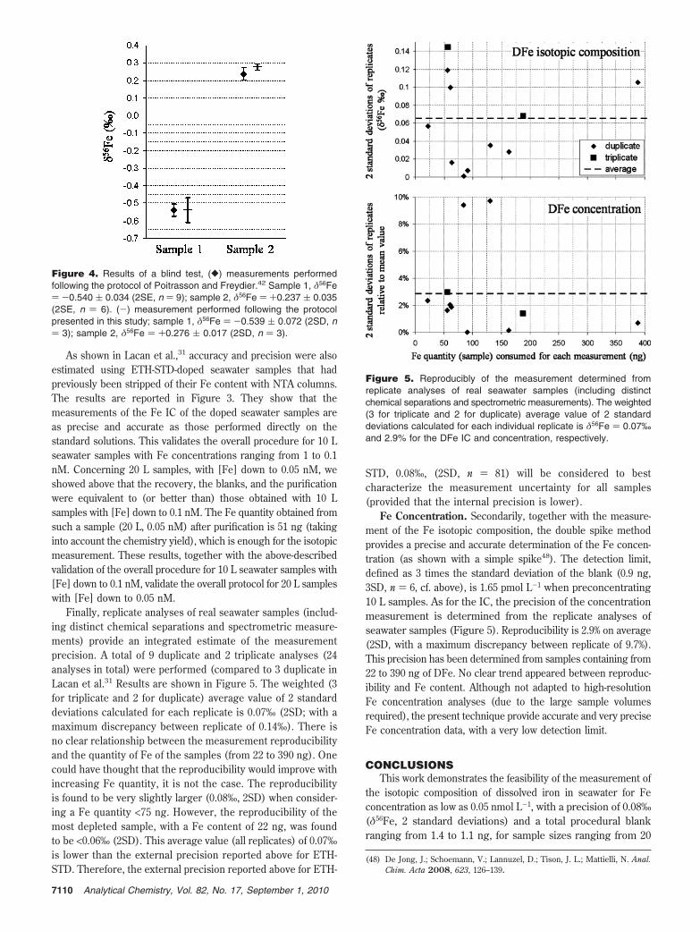
Finally, replicate analyses of real seawater samples (includ-ing distinct chemical separations and spectrometric measure-ments) provide an integrated estimate of the measurementprecision. A total of 9 duplicate and 2 triplicate analyses (24analyses in total) were performed (compared to 3 duplicate inLacan et al.31 Results are shown in Figure 5. The weighted (3for triplicate and 2 for duplicate) average value of 2 standarddeviations calculated for each replicate is 0.07‰ (2SD; with amaximum discrepancy between replicate of 0.14‰). There isno clear relationship between the measurement reproducibilityand the quantity of Fe of the samples (from 22 to 390 ng). Onecould have thought that the reproducibility would improve withincreasing Fe quantity, it is not the case. The reproducibilityis found to be very slightly larger (0.08‰, 2SD) when consider-ing a Fe quantity <75 ng. However, the reproducibility of themost depleted sample, with a Fe content of 22 ng, was foundto be <0.06‰ (2SD). This average value (all replicates) of 0.07‰is lower than the external precision reported above for ETH-STD. Therefore, the external precision reported above for ETH-

STD, 0.08‰, (2SD, n ) 81) will be considered to bestcharacterize the measurement uncertainty for all samples(provided that the internal precision is lower).

Fe Concentration. Secondarily, together with the measure-ment of the Fe isotopic composition, the double spike methodprovides a precise and accurate determination of the Fe concen-tration (as shown with a simple spike48). The detection limit,defined as 3 times the standard deviation of the blank (0.9 ng,3SD, n ) 6, cf. above), is 1.65 pmol L-1 when preconcentrating10 L samples. As for the IC, the precision of the concentrationmeasurement is determined from the replicate analyses ofseawater samples (Figure 5). Reproducibility is 2.9% on average(2SD, with a maximum discrepancy between replicate of 9.7%).This precision has been determined from samples containing from22 to 390 ng of DFe. No clear trend appeared between reproduc-ibility and Fe content. Although not adapted to high-resolutionFe concentration analyses (due to the large sample volumesrequired), the present technique provide accurate and very preciseFe concentration data, with a very low detection limit.

CONCLUSIONSThis work demonstrates the feasibility of the measurement of

the isotopic composition of dissolved iron in seawater for Feconcentration as low as 0.05 nmol L-1, with a precision of 0.08‰(δ56Fe, 2 standard deviations) and a total procedural blankranging from 1.4 to 1.1 ng, for sample sizes ranging from 20

(48) De Jong, J.; Schoemann, V.; Lannuzel, D.; Tison, J. L.; Mattielli, N. Anal.Chim. Acta 2008, 623, 126–139.

Figure 4. Results of a blind test, ([) measurements performedfollowing the protocol of Poitrasson and Freydier.42 Sample 1, δ56Fe) -0.540 ( 0.034 (2SE, n ) 9); sample 2, δ56Fe ) +0.237 ( 0.035(2SE, n ) 6). (-) measurement performed following the protocolpresented in this study; sample 1, δ56Fe ) -0.539 ( 0.072 (2SD, n) 3); sample 2, δ56Fe ) +0.276 ( 0.017 (2SD, n ) 3).

Figure 5. Reproducibly of the measurement determined fromreplicate analyses of real seawater samples (including distinctchemical separations and spectrometric measurements). The weighted(3 for triplicate and 2 for duplicate) average value of 2 standarddeviations calculated for each individual replicate is δ56Fe ) 0.07‰and 2.9% for the DFe IC and concentration, respectively.

7110 Analytical Chemistry, Vol. 82, No. 17, September 1, 2010

to 2 L respectively, which converted into Fe concentrationscorrespond to blank contributions of 0.001 to 0.010 nmol L-1,respectively.

Iron is preconcentrated using a column of nitriloacetic acidsuperflow resin and purified using a column of AG 1-×4 anionexchange resin. The preconcentration procedure has the advan-tage of being entirely closed, which prevents contamination fromthe air. Although not tested so far, it could therefore be performedonboard.

The isotopic ratios are measured with a MC-ICPMS Neptune,coupled with a desolvator (Aridus II or better Apex-Q), using a57Fe-58Fe double spike mass bias correction. The range ofvariation observed in the ocean so far being of about 2.5‰,the measurement precision is only about 3% of this range. Suchmeasurements therefore allow for the detection of small

variations in the oceanic dissolved Fe isotopic composition andthus open new perspectives for the study of the many facetsof the oceanic Fe cycle, such as its sources and sinks and itsredox and/or biological cycles.

ACKNOWLEDGMENTThe CNRS (French National Center for Scientific Research)

is thanked for supporting this study. Candaudap is thanked forhis help with the quadrupole ICPMS. We thank L. Coppola forproviding the Dyfamed seawater. We thank three anonymousreviewers, who greatly helped improve this manuscript.

Received for review January 28, 2010. Accepted June 25,2010.

AC1002504

7111Analytical Chemistry, Vol. 82, No. 17, September 1, 2010