Embed Size (px)
Citation preview
HIGH PRECISION ABSOLUTE GRAVITY
GRADIOMETRY WITH ATOM INTERFEROMETRY
a dissertation
submitted to the department of physics
and the committee on graduate studies
of stanford university
in partial fulfillment of the requirements
for the degree of
doctor of philosophy
By
Jeffrey Michael McGuirk
September 2001

c© Copyright 2001 by Jeffrey Michael McGuirk
All Rights Reserved
ii
I certify that I have read this dissertation and that in
my opinion it is fully adequate, in scope and quality, as
a dissertation for the degree of Doctor of Philosophy.
Mark Kasevich(Principal Adviser)
I certify that I have read this dissertation and that in
my opinion it is fully adequate, in scope and quality, as
a dissertation for the degree of Doctor of Philosophy.
Steven Chu(Department of Physics and Applied Physics)
I certify that I have read this dissertation and that in
my opinion it is fully adequate, in scope and quality, as
a dissertation for the degree of Doctor of Philosophy.
John Turneaure(Department of Physics)
Approved for the University Committee on Graduate
Studies:
iii

iv
Abstract
An absolute gravity gradiometer was demonstrated using atom interference tech-
niques. This is the first realization of an gradiometer which uses an absolute standard
for its calibration. A gravity gradiometer measures spatial changes in the gravita-
tional field over a fixed baseline by making simultaneous acceleration measurements
with two spatially separate accelerometers. The gradiometer has a differential sen-
sitivity of 4 × 10⁻⁹ g in 1 s and a differential accuracy of 10−9 g. This is the best
gradiometer accuracy reported to date and the sensitivity competes favorably with
existing state-of-the-art instruments. A proof-of-principle measurement of the grav-
ity gradient of a small test mass was made leading towards a precision measurement
of the gravitational constant. The performance was characterized on a vibrationally
noisy reference platform, testing the ability of the gradiometer to reject common-
mode accelerations. Techniques for extracting gradient information were explored.
Applications of sensitive and accurate gravity gradiometers include tests of general
relativity, studies of the gravitational constant, navigation, and geophysical studies.
The principle behind the measurement is as follows: proof masses for the two ac-
celerometers consist of two ensembles of laser-cooled cesium atoms whose acceleration
is measured by an interferometer sequence. The interferometer is comprised of light
pulses in a π/2−π−π/2 pulse sequence which acts to divide, deflect, and recombine
each atomic wavepacket. The final state of the atom depends on the inertial forces
experienced by the atom during its trajectory through the interferometer. The two
simultaneous acceleration measurements are subtracted to produce a gravity gradi-
ent. This technique is advantageous because it offers intrinsic absolute calibration,
robust operation, and uniformity of proof masses.
v
Acknowledgements
I am deeply grateful to my advisor Mark Kasevich. In addition to being a gifted
physicist who taught me an amazing amount of physics, Mark has both the vision
to pursue interesting ideas and the experimental ability to carry them out. On top
of physics, it has just been fun to work with Mark. I cannot forget the opportunity
he allowed me to live on both coasts. Along the way, I have been fortunate to work
with a number of talented people. Dean Haritos and Philippe Bouyer helped build
the experiment at Stanford. During his post-doc, Mike Snadden assisted with the
proof-of-principle work at Stanford, helped during the move to Yale in 1997, and was
instrumental in the steps leading to the current device performance. Also, in his spare
time, Mike wrote 25,000 lines of computer code to control the timing and data acqui-
sition. Greg Foster and Jeff Fixler helped develop the data extraction routines and
demonstrate the performance of the gradiometer, and they have smoothly assumed
the running of the experiment for the measurement of G. Post-doc Kai Bongs and
students Romain Launay and Neelima Sehgal developed the details of the interfer-
ometer theory and enlightened me with many discussions. I am also thankful for the
general laboratory expertise of my colleagues Brian Anderson and Todd Gustavson,
and for many useful discussions with Kurt Gibble. The work in this dissertation was
funded by ONR, NASA, and NRO. My time in Stanford and New Haven was made
more enjoyable and my sanity was maintained with the help of Dean, Mike, Todd,
Brian, Jamie Kerman, and the Saeco Magic de Luxe. Finally I wish to thank my
family for their support.
vi
Contents
Abstract v
Acknowledgements vi
1 Introduction 1
1.1 Introduction . . . . . . . . . . . . . . . . . . . . . . . . . . . . . . . . 1
1.2 Gradiometry and the equivalence principle . . . . . . . . . . . . . . . 2
1.3 Laser manipulation of atoms . . . . . . . . . . . . . . . . . . . . . . . 3
1.4 Atom interferometry . . . . . . . . . . . . . . . . . . . . . . . . . . . 4
1.5 Overview . . . . . . . . . . . . . . . . . . . . . . . . . . . . . . . . . . 5
2 Gravity Gradiometry 6
2.1 Gradient tensor . . . . . . . . . . . . . . . . . . . . . . . . . . . . . . 6
2.2 Gradient units . . . . . . . . . . . . . . . . . . . . . . . . . . . . . . . 7
2.3 Gradiometer applications . . . . . . . . . . . . . . . . . . . . . . . . . 8
2.3.1 Inertial navigation . . . . . . . . . . . . . . . . . . . . . . . . 8
2.3.2 Subsurface mass anomalies . . . . . . . . . . . . . . . . . . . . 9
2.3.3 Gravitational constant . . . . . . . . . . . . . . . . . . . . . . 11
2.3.4 Tests of General Relativity . . . . . . . . . . . . . . . . . . . . 14
2.3.5 Fifth force experiments . . . . . . . . . . . . . . . . . . . . . . 14
2.4 Alternate gradiometer technologies . . . . . . . . . . . . . . . . . . . 15
2.4.1 Mass-spring gradiometers . . . . . . . . . . . . . . . . . . . . 15
2.4.2 Superconducting instruments . . . . . . . . . . . . . . . . . . 16
2.4.3 Falling cornercube gradiometer . . . . . . . . . . . . . . . . . 16
vii
2.4.4 Absolute gradiometry . . . . . . . . . . . . . . . . . . . . . . . 17
3 Laser Cooling and Trapping 18
3.1 Atomic structure . . . . . . . . . . . . . . . . . . . . . . . . . . . . . 18
3.2 Two-level atoms . . . . . . . . . . . . . . . . . . . . . . . . . . . . . . 19
3.3 Optical forces . . . . . . . . . . . . . . . . . . . . . . . . . . . . . . . 21
3.3.1 Scattering force . . . . . . . . . . . . . . . . . . . . . . . . . . 21
3.3.2 Dipole force . . . . . . . . . . . . . . . . . . . . . . . . . . . . 23
3.4 Magnetic forces . . . . . . . . . . . . . . . . . . . . . . . . . . . . . . 23
3.5 Laser cooling . . . . . . . . . . . . . . . . . . . . . . . . . . . . . . . 24
3.5.1 Doppler cooling . . . . . . . . . . . . . . . . . . . . . . . . . . 24
3.5.2 Polarization gradient cooling . . . . . . . . . . . . . . . . . . . 26
3.6 Magneto-optical trapping . . . . . . . . . . . . . . . . . . . . . . . . . 27
3.6.1 Trap loading . . . . . . . . . . . . . . . . . . . . . . . . . . . . 29
3.6.2 Atomic fountains . . . . . . . . . . . . . . . . . . . . . . . . . 30
3.7 Two-photon stimulated Raman transitions . . . . . . . . . . . . . . . 31
3.8 Atom detection . . . . . . . . . . . . . . . . . . . . . . . . . . . . . . 36
3.9 Experiment synopsis . . . . . . . . . . . . . . . . . . . . . . . . . . . 37
4 Atom Interferometry 39
4.1 Intuitive analogy . . . . . . . . . . . . . . . . . . . . . . . . . . . . . 40
4.2 Interferometer description . . . . . . . . . . . . . . . . . . . . . . . . 41
4.3 Wavepacket overlap phase . . . . . . . . . . . . . . . . . . . . . . . . 43
4.4 Laser phase . . . . . . . . . . . . . . . . . . . . . . . . . . . . . . . . 44
4.4.1 Frequency term . . . . . . . . . . . . . . . . . . . . . . . . . . 45
4.4.2 Initial phase . . . . . . . . . . . . . . . . . . . . . . . . . . . . 46
4.5 Free propagation phase . . . . . . . . . . . . . . . . . . . . . . . . . . 47
4.5.1 Path integral formalism . . . . . . . . . . . . . . . . . . . . . 47
4.5.2 Perturbative approach . . . . . . . . . . . . . . . . . . . . . . 49
4.6 Nonuniform acceleration fields . . . . . . . . . . . . . . . . . . . . . . 50
4.6.1 Exact solution . . . . . . . . . . . . . . . . . . . . . . . . . . . 50
4.6.2 Gravity gradients . . . . . . . . . . . . . . . . . . . . . . . . . 51
viii
4.6.3 Rotations . . . . . . . . . . . . . . . . . . . . . . . . . . . . . 52
4.7 Limitations to the theory . . . . . . . . . . . . . . . . . . . . . . . . . 53
4.8 Application to gradiometry . . . . . . . . . . . . . . . . . . . . . . . . 55
5 Experimental Apparatus 57
5.1 Apparatus overview . . . . . . . . . . . . . . . . . . . . . . . . . . . . 57
5.2 Vacuum system . . . . . . . . . . . . . . . . . . . . . . . . . . . . . . 57
5.2.1 Motivation for vacuum . . . . . . . . . . . . . . . . . . . . . . 57
5.2.2 Vacuum chamber design and preparation . . . . . . . . . . . . 59
5.2.3 Chamber evacuation . . . . . . . . . . . . . . . . . . . . . . . 62
5.3 Laser system . . . . . . . . . . . . . . . . . . . . . . . . . . . . . . . 63
5.3.1 Master laser . . . . . . . . . . . . . . . . . . . . . . . . . . . . 63
5.3.2 Laser amplifiers . . . . . . . . . . . . . . . . . . . . . . . . . . 65
5.3.3 Optical fiber system . . . . . . . . . . . . . . . . . . . . . . . 68
5.4 Laser cooled atomic sources . . . . . . . . . . . . . . . . . . . . . . . 69
5.5 State preparation . . . . . . . . . . . . . . . . . . . . . . . . . . . . . 71
5.5.1 Optical pumping . . . . . . . . . . . . . . . . . . . . . . . . . 72
5.5.2 Composite pulse techniques . . . . . . . . . . . . . . . . . . . 74
5.6 Atom interferometer . . . . . . . . . . . . . . . . . . . . . . . . . . . 76
5.6.1 Raman lasers . . . . . . . . . . . . . . . . . . . . . . . . . . . 76
5.6.2 Beam delivery . . . . . . . . . . . . . . . . . . . . . . . . . . . 79
5.6.3 Propagation reversal . . . . . . . . . . . . . . . . . . . . . . . 82
5.6.4 Raman beam parameters . . . . . . . . . . . . . . . . . . . . . 83
5.6.5 Interferometer operation . . . . . . . . . . . . . . . . . . . . . 85
5.7 Detection system . . . . . . . . . . . . . . . . . . . . . . . . . . . . . 85
5.7.1 Background . . . . . . . . . . . . . . . . . . . . . . . . . . . . 85
5.7.2 Detection apparatus . . . . . . . . . . . . . . . . . . . . . . . 87
5.7.3 Detection system performance . . . . . . . . . . . . . . . . . . 91
5.7.4 Noise analysis . . . . . . . . . . . . . . . . . . . . . . . . . . . 93
5.8 Vibration isolation subsystem . . . . . . . . . . . . . . . . . . . . . . 94
5.8.1 Mechanical design . . . . . . . . . . . . . . . . . . . . . . . . . 95
ix
5.8.2 DSP servo system . . . . . . . . . . . . . . . . . . . . . . . . . 96
5.9 Microwave generation . . . . . . . . . . . . . . . . . . . . . . . . . . . 96
6 Results 99
6.1 Proof-of-principle results . . . . . . . . . . . . . . . . . . . . . . . . . 99
6.2 Signal extraction . . . . . . . . . . . . . . . . . . . . . . . . . . . . . 101
6.2.1 Normalization . . . . . . . . . . . . . . . . . . . . . . . . . . . 101
6.2.2 Interference fringe fitting . . . . . . . . . . . . . . . . . . . . . 102
6.2.3 Magnetic phase shifting . . . . . . . . . . . . . . . . . . . . . 104
6.2.4 Gaussian elimination reduction . . . . . . . . . . . . . . . . . 106
6.2.5 Circle fitting . . . . . . . . . . . . . . . . . . . . . . . . . . . . 108
6.2.6 Ellipse fitting . . . . . . . . . . . . . . . . . . . . . . . . . . . 111
6.2.7 Summary of data extraction methods . . . . . . . . . . . . . . 115
6.3 Sensitivity characterization . . . . . . . . . . . . . . . . . . . . . . . . 116
6.3.1 Noise . . . . . . . . . . . . . . . . . . . . . . . . . . . . . . . . 117
6.3.2 Proof-of-principle mass detection . . . . . . . . . . . . . . . . 118
6.4 Accuracy estimation . . . . . . . . . . . . . . . . . . . . . . . . . . . 118
6.4.1 Tidal measurement . . . . . . . . . . . . . . . . . . . . . . . . 118
6.4.2 Allan variance . . . . . . . . . . . . . . . . . . . . . . . . . . . 120
6.4.3 Gravitational constant measurement . . . . . . . . . . . . . . 122
6.5 Immunity to environmental noise . . . . . . . . . . . . . . . . . . . . 124
6.5.1 Linear acceleration . . . . . . . . . . . . . . . . . . . . . . . . 124
6.5.2 Rotation . . . . . . . . . . . . . . . . . . . . . . . . . . . . . . 127
7 Discussion 130
7.1 Performance Limits . . . . . . . . . . . . . . . . . . . . . . . . . . . . 130
7.1.1 SNR limits . . . . . . . . . . . . . . . . . . . . . . . . . . . . . 130
7.1.2 Rotations . . . . . . . . . . . . . . . . . . . . . . . . . . . . . 131
7.2 Related methods . . . . . . . . . . . . . . . . . . . . . . . . . . . . . 133
7.2.1 Large area interferometers . . . . . . . . . . . . . . . . . . . . 133
7.2.2 Interferometer comparisons . . . . . . . . . . . . . . . . . . . 139
7.2.3 Multi-loop interferometers . . . . . . . . . . . . . . . . . . . . 142
x

7.2.4 Curvature measurements . . . . . . . . . . . . . . . . . . . . . 145
7.2.5 Multi-axis gradiometers . . . . . . . . . . . . . . . . . . . . . 146
8 Conclusion 149
8.1 Future enhancements . . . . . . . . . . . . . . . . . . . . . . . . . . . 149
8.2 Future measurements . . . . . . . . . . . . . . . . . . . . . . . . . . . 151
A Physical parameters of Cs 154
B Digital control loops 156
Bibliography 159
xi

List of Tables
A.1 Properties of Cs . . . . . . . . . . . . . . . . . . . . . . . . . . . . . . 154
B.1 Vibration isolation system filter bandwidths and gains. . . . . . . . . 158
xii
List of Figures
1.1 Conceptual representation of a gradiometer . . . . . . . . . . . . . . . 1
2.1 Gravity gradient of an underground structure . . . . . . . . . . . . . 10
2.2 Recent measurements of the gravitational constant . . . . . . . . . . 13
3.1 Schematic representation of the scattering force . . . . . . . . . . . . 22
3.2 Illustration of Doppler cooling . . . . . . . . . . . . . . . . . . . . . . 25
3.3 Illustration of an atom in a 1D MOT . . . . . . . . . . . . . . . . . . 28
3.4 Schematic depictions of 3D MOT configurations . . . . . . . . . . . . 32
3.5 Energy level diagram for Raman transitions . . . . . . . . . . . . . . 34
4.1 Conceptual picture of a gravity measurement . . . . . . . . . . . . . . 40
4.2 Recoil diagram of the interferometer sequence . . . . . . . . . . . . . 42
4.3 Interferometer path overlap in the presence of gradients . . . . . . . . 44
5.1 Picture of the gravity gradiometer apparatus . . . . . . . . . . . . . . 58
5.2 Vacuum chambers . . . . . . . . . . . . . . . . . . . . . . . . . . . . . 60
5.3 Spectral purity of tapered amplifiers . . . . . . . . . . . . . . . . . . 66
5.4 Block diagram of trapping laser system . . . . . . . . . . . . . . . . . 68
5.5 Launching of cold atoms . . . . . . . . . . . . . . . . . . . . . . . . . 71
5.6 Sequence of state preparation and interferometer pulses . . . . . . . . 73
5.7 Transfer efficiency of composite pulses . . . . . . . . . . . . . . . . . 75
5.8 Raman beam geometry . . . . . . . . . . . . . . . . . . . . . . . . . . 78
5.9 Block diagram of the Raman laser system . . . . . . . . . . . . . . . 79
5.10 Rejection of magnetic phase shifts with Raman propagation reversal . 83
xiii

5.11 Interferometer contrast simulation . . . . . . . . . . . . . . . . . . . . 84
5.12 Schematic representation of the detection apparatus . . . . . . . . . . 88
5.13 Study of optimal detection parameters . . . . . . . . . . . . . . . . . 89
5.14 Shot noise limited detection . . . . . . . . . . . . . . . . . . . . . . . 92
5.15 Schematic view of the vibration isolation system . . . . . . . . . . . . 95
5.16 Performance of the vibration isolation system . . . . . . . . . . . . . 97
6.1 Proof-of-principle Earth gradient measurement . . . . . . . . . . . . . 100
6.2 Sinusoidal least squares fits to interference fringes . . . . . . . . . . . 103
6.3 Decrease of SNR with phase mismatch . . . . . . . . . . . . . . . . . 105
6.4 Data reduction using Gaussian elimination method . . . . . . . . . . 108
6.5 Data analysis using deviations from a circle . . . . . . . . . . . . . . 110
6.6 Ellipse fitting of data . . . . . . . . . . . . . . . . . . . . . . . . . . . 113
6.7 Calibration of ellipse fitting routine . . . . . . . . . . . . . . . . . . . 114
6.8 Comparison of interference fringes with vibration isolation . . . . . . 117
6.9 Measurement of the gradient of a small test mass . . . . . . . . . . . 119
6.10 Gravitational tidal signals . . . . . . . . . . . . . . . . . . . . . . . . 120
6.11 Allan variance of gradiometer data . . . . . . . . . . . . . . . . . . . 121
6.12 Precision lead test masses . . . . . . . . . . . . . . . . . . . . . . . . 122
6.13 Linear acceleration test . . . . . . . . . . . . . . . . . . . . . . . . . . 125
6.14 Interferometer transfer function for vibrational phase noise . . . . . . 126
6.15 Platform tilt test . . . . . . . . . . . . . . . . . . . . . . . . . . . . . 128
6.16 Effect of rotations on interferometer contrast . . . . . . . . . . . . . . 129
7.1 6hk interferometer recoil diagram . . . . . . . . . . . . . . . . . . . . 133
7.2 Schematic representation of multiple pulse interferometers . . . . . . 134
7.3 Comparison of phase shift for 2hk and 6hk interferometers . . . . . . 137
7.4 Interference fringes using a 6hk interferometer . . . . . . . . . . . . . 138
7.5 Recoil diagrams for multiple loop interferometers . . . . . . . . . . . 144
7.6 Triple-loop interference fringes . . . . . . . . . . . . . . . . . . . . . . 146
7.7 Full gradient tensor measurement configuration . . . . . . . . . . . . 147
xiv
A.1 Energy level diagram for 133Cs . . . . . . . . . . . . . . . . . . . . . . 155
B.1 Transfer function of the SHP-voice coil system . . . . . . . . . . . . . 157
B.2 Comparison of digital filters . . . . . . . . . . . . . . . . . . . . . . . 158
xv
Chapter 1
Introduction
1.1 Introduction
Gravity gradiometry is the study of spatial changes in the gravitational field over a
known distance. A gravity gradiometer measures the spatial rate of change of the
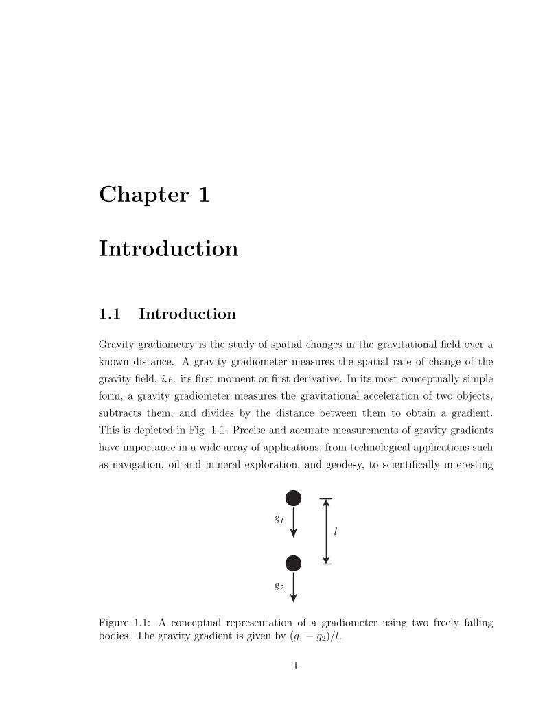
gravity field, i.e. its first moment or first derivative. In its most conceptually simple
form, a gravity gradiometer measures the gravitational acceleration of two objects,
subtracts them, and divides by the distance between them to obtain a gradient.
This is depicted in Fig. 1.1. Precise and accurate measurements of gravity gradients
have importance in a wide array of applications, from technological applications such
as navigation, oil and mineral exploration, and geodesy, to scientifically interesting
lg1
g2
Figure 1.1: A conceptual representation of a gradiometer using two freely fallingbodies. The gravity gradient is given by (g1 − g2)/l.
1
2 CHAPTER 1. INTRODUCTION
applications including a precision measurement of the gravitational constant, tests
of general relativity, and searches for new physics in the form of a fifth force. The
gravity gradiometer described in this dissertation has the potential to meet many of
these applications, based on its demonstrated differential sensitivity of 4 × 10⁻⁹g in
1 s and differential accuracy of less than 10−9g.
1.2 Gradiometry and the equivalence principle
At first glance, it might seem that a gravity gradient is an odd quantity to measure.
After all, the quantity of interest in most of the applications listed is gravity itself.
The reason why gravity gradients are important lies in the equivalence principle.
Einstein, in his 1911 formulation of equivalence [1], states that
“This assumption of exact physical equivalence makes it impossible for us
to speak of the absolute acceleration of the system of reference, just as the
usually theory of relativity forbids us to talk of the absolute velocity of a
system; and it makes the equal falling of all bodies in a gravitational field
seem a matter of course.”
In other words, when making a gravity measurement, it is impossible to differentiate
the gravitational acceleration experienced by the proof mass from the acceleration of
the reference frame of the measurement. The reference frame of the measurement is
defined by the platform on which the acceleration read-out devices1 are placed. If this
reference frame is accelerating, due to vibrations or motion of the vehicle transporting
the device, then the measured acceleration will include these offsets and noise from
the accelerating reference platform. For this reason, gravimetry is fundamentally
challenged by its sensitivity to platform vibrations. A sensitive gravimeter requires
a quiet reference platform, otherwise the noise from platform vibrations limits the
sensitivity.
It was realized that a gravity gradiometer can circumvent the problem of plat-
form vibrations. By making simultaneous acceleration measurements at two spatially
1The acceleration sensitive components can be capacitors, superconducting coils, photodetectors,mirrors, etc. depending on the measurement method.
1.3. LASER MANIPULATION OF ATOMS 3
separated locations a differential measurement of the gravity field can be made. If
both these measurements are made with respect to the same reference frame, and if
the two accelerometers experience common vibrations, then all accelerations of the
reference platform can be removed as a common-mode. Measuring gravity gradients
then can be an effective tool to circumvent the noise limits of a vibrationally noisy
platform2. The key to successful gravity gradiometry lies in ensuring that the two
accelerometers are tightly coupled so as to only have common-mode vibrations. Tra-
ditionally, there has been a compromise between intrinsic gradiometer sensitivity and
noise suppression in gravity gradiometers. This tradeoff is because expanding the
baseline distance between the two accelerometers linearly increases the sensitivity to
gradients, but all previously demonstrated devices require rigid mechanical coupling
between accelerometers for good common-mode vibration suppression, which becomes
difficult to do over large baselines. The device presented in this dissertation is fun-
damentally different. It uses light pulses effectively to couple the two accelerometers
together and requires no rigid coupling between accelerometers to maintain common-
mode performance3. By removing this constraint, the baseline can be made arbitrarily
large, and the sensitivity scales accordingly.
1.3 Laser manipulation of atoms
The key enabling technologies for this gravity gradiometer are the techniques of ma-
nipulating atoms using lasers that were pioneered over the last 20 years. In the mid to
late 1970s, several proposals for slowing atoms with optical forces were made [2, 3],
but it was not until 1982 that it was first observed that the the motion of atoms
could be damped by transferring momentum to them from optical fields [4]. In 1986,
this advance was taken one step further with the invention of “optical molasses” [5].
An optical molasses is a configuration of laser beams that acts to damp the motion
of atoms in all directions by transferring kinetic energy to the optical field. Based
2The definition of “noisy” depends on the scale of the measurement, and for some purposes,platforms with accelerations as small as 10−9g are considered noisy.
3The light pulses couple vibrations to the two accelerometers identically, and these common-modespurious accelerations are removed during the data reduction.
4 CHAPTER 1. INTRODUCTION
on this technique, atoms could be cooled to temperature of several µK, where their
velocities are slow enough to perform experiments requiring long interrogation times.
Furthermore a way of producing a dense cloud with large numbers of laser-cooled
atoms was pioneered by adding a magnetic field to the molasses to produce a localiz-
ing restoring force [6]. Such a configuration is called a magneto-optical trap (MOT),
and can be used to produce as many as 1010 ultra cold atoms in a region with a
size of ∼ 1 mm or less. The MOT has become the workhorse of modern atomic
physics, as it has proven to be an extremely robust source of dense, cold atoms that
is straightforward to produce. In recognition of these achievements, the Nobel Prize
in Physics was awarded in 1997 to three of the pioneers of laser cooling and trapping:
Chu, Cohen-Tannoudji, and Phillips [7].
1.4 Atom interferometry
Ramsey developed an interferometer for atoms based on microwave fields (the “sep-
arated oscillatory field” method) in the 1950s [8]. Building on early work in neutron
interferometry [9, 10], there were several proposals to use neutral atoms as inertial
force sensors in atom interferometers [11, 12]. Analogous to neutron scattering from
silicon crystals, atom interference was shown using using narrow mechanical gratings
to diffract the atom into two separate wavepackets and then to diffract them back to
overlap and interfere [13]. More interestingly, soon thereafter, atom interference was
demonstrating using not mechanical gratings to diffract the atoms, but optical fields
in the form of two-photon stimulated Raman transitions [14, 15]. Optical fields were
used to divide the atom into two wavepackets, direct the wavepackets back towards
each other after a drift period, and finally to recombine the wavepackets at a location
where their interference could be observed. These optical elements are analogous
to the beamsplitters and the mirrors used in a standard Michelson interferometer.
Soon after, a light-pulse-based interferometer sensitive to gravitational acceleration
on the freely falling atoms was demonstrated in 1992 [16]. In the following years
a similar-in-concept atom interferometer gyroscope was demonstrated [17], sensitive
enhancements to the original gravimeter idea were made [18], and the gravity gradient
1.5. OVERVIEW 5
sensitive interferometer presented herein was demonstrated [19].
1.5 Overview
The format of this dissertation is as follows. Chapter 2 contains an introduction to the
study of gravity gradients, including interesting applications of gradiometry as well
as brief descriptions of existing gradiometers. A review of the fundamental concepts
of the behavior of atoms in optical fields, particularly related to laser cooling and
trapping and two-photon Raman transitions, is the subject of Chapter 3. Chapter 4
provides a detailed discussion on the nature of the atom interferometers and the effects
of inertial forces on the atomic phases in interferometers. The experimental apparatus
is described in Chapter 5. Chapter 6 presents the results of the experiments and
includes a detailed discussion on the extraction of phase information from the data.
Chapter 7 provides a discussion of the limits of the gravity gradiometer, proposes
several related interferometer schemes, and compares this work with related methods.
Finally, Chapter 8 concludes with possible future experimental enhancements as well
as brief descriptions of potential future measurements.
Chapter 2
Gravity Gradiometry
The purpose of this section is to discuss several aspects of gravity gradiometry. Ex-
isting gravity gradiometers will be described. The need for sensitive and accurate
gradiometer is elucidated. The applications described in section 2.3 are by no means
an exhaustive listing of the technical and scientific applications of a precise absolute
gravity gradiometer. They are merely meant as descriptions of several of the more
important applications and some of the new physics that might come out of such
studies of gravity requiring unprecedented levels of accuracy and precision.
2.1 Gradient tensor
The gravity gradient is a tensor quantity. The gradient tensor is a three-by-three
matrix whose components are the derivative of the three components of the gravity
vector (x, y, and z) with respect to each spatial direction:
T = ∇g =
∂gx
∂x∂gx
∂y∂gx
∂z∂gy
∂x∂gy
∂y∂gy
∂z∂gz
∂x∂gz
∂y∂gz
∂z
. (2.1)
The notation gxx is often used to denote ∂gx
∂x, and so forth. There are nine components
to the gradient tensor, however only five of them are independent components. The
6
2.2. GRADIENT UNITS 7
tensor is a symmetric tensor, i.e. Tij = Tji. Additionally, the trace is equal to
zero so knowledge of two diagonal components determines the third. In order to
characterize completely the gravitational field, five components of the tensor must be
measured, two diagonal components and three off-diagonal components. In practice
however, enough information is often carried primarily in one component, and then
a one-axis device is usually sufficient. The device presented herein is a one-axis
gradiometer, however in section 7.2.5 various schemes for constructing multi-axis
devices are discussed.
2.2 Gradient units
The fundamental unit of gravity gradiometry is the Eotvos, named after the Hun-
garian physicist credited with making the first gravity gradient measurements [20],
1 E = 10−9 s−2, or 1 E 10−10 g/m, where g is the gravitational acceleration near
the Earth’s surface and is 9.8 m/s2. The Eotvos is an exceedingly small unit, and
measurements with accuracies of 1 E or less have not been achieved prior to this work.
As a point of reference, the Earth’s gravity gradient with increasing altitude near the
surface is ∼ 3000 E1. It is a somewhat nonintuitive unit, and often it is preferable
to think of gravity gradiometers in terms of differential acceleration measurements,
which are typically referred to as a differential acceleration divided by a baseline, i.e.
as g/m. In these units, the Earth’s gradient is ∼ 3×10⁻⁷ g/m. To further complicate
the picture, the CGS unit of acceleration is the gal, 1 gal = 1 cm/s2 10−3 g. Sensi-
tive acceleration measurements are discussed in terms of µgal, and 1 E = 0.1 µgal/m.
This unit is the unit of choice in the navigation and geophysics communities, but will
not be used here.
The sensitivity of the gradiometer is typically quoted in units of E/√
Hz or g/√
Hz.
These units are meant to be the sensitivities for a white noise limited process where
the precision scales inversely as the square root of the measurement time [21]. For
example, this means that a 1 E/√
Hz device has a raw noise of 1 E in a 1 Hz bandwidth,
giving a precision of about 1 E in 1 s, and a precision of about 0.1 E in 100 s if it has
1The Earth’s gradient is obtained from the derivative of the inverse square law of gravity.
8 CHAPTER 2. GRAVITY GRADIOMETRY
white noise properties. It is the case that the gradiometer presented herein has white
noise scaling over a range of time greater than 103 s before the sensitivity begins to
roll off. This is discussed in section 6.4.
2.3 Gradiometer applications
There is a host of applications for gravity gradiometry. Typically, knowledge of grav-
ity is required for a number of field applications. These applications almost always
include operation on a noisy platform, which severely hampers gravitational accel-
eration measurements. For this reason, gravity gradiometry is useful. Additionally
for precision scientific measurements, gravity gradiometry lessens the constraints on
the level of the exact knowledge of the local gravitational field and its variations
from tides, ocean loading, post-glacial rebound, near-field masses, etc. [22]. This
section describes some of the major applications for gravity gradiometry and related
measurements that could be made with the atom interferometer presented in this
dissertation. First technological applications are described, and then precision mea-
surements of scientific interest are described.
2.3.1 Inertial navigation
A long-standing goal of the navigation community has been the development of a
quiet, self-contained inertial navigation system. Inertial navigation consists of mea-
suring the inertial forces experienced by an object, specifically rotations and accel-
erations, and using these forces to determine completely the trajectory and location
of the object from a known initial position [23]. The Global Positioning System
(GPS) is an excellent navigation tool, as are active methods such as radar and sonar,
however there are a number of environments where GPS is unavailable and active
methods are unavailable or undesirable. In these instances, inertial navigation is key.
In navigation grade inertial navigation systems2 the position estimate obtained from
2Navigation grade systems require higher performance than tactical grade systems due to longertimescales involved.
2.3. GRADIOMETER APPLICATIONS 9
the on-board accelerometers and gyroscopes is typically limited by knowledge of lo-
cal gravity g, particularly near large gravitational anomalies such as mountains and
valleys, as these anomalies can perturb the perceived platform vertical as determined
by the gyroscopes. In these instances, an onboard gravity gradiometer could correct
the inertial navigation system’s position estimate. The positioning obtained from
GPS is limited by the knowledge of the position of the satellites themselves. Exact
knowledge of the Earth’s gravitational field dynamically measured onboard each GPS
satellite operating at a differential sensitivity ∼ 10−9 g/√
Hz would allow for correc-
tion of orbital perturbations from the Earth’s non-uniform gravity field, i.e. periodic
orbital corrections from ground-based measurements of the satellite orbits would not
be required.
2.3.2 Subsurface mass anomalies
Another application well-suited to gravity gradiometers is the detection of subsurface
mass anomalies. Nonuniform densities below the surface of the Earth cause gravita-
tional anomalies through changes in both the local gravity g and the gravity gradient
∇g. Examples of nonuniformities include oil and mineral deposits, water reservoir
levels, and underground tunnels and bunkers. Recently, a measurement of two large,
hollowed out underground chambers was made by using the mechanical gradiometer
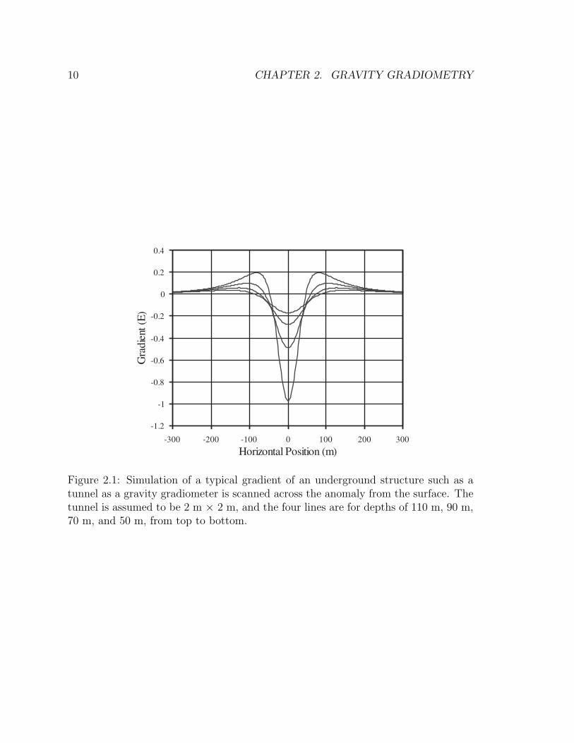
described in section 2.4.1. As a gradiometer is moved across a subsurface anomaly,
a characteristic signal is seen (see Fig. 2.1). The altitude at which the gradiometer
makes measurements (i.e. land-based, airborne, or satellite) as well as the depth of
the anomaly determine the spatial resolution at which the anomaly may be detected.
The spatial resolution of the gravity gradient measurements can be understood by
expressing the gravity field of the Earth as an expansion of spherical harmonics at the
altitude of the measurement. For optimal detection of features, the wavelengths of
the primary components in the spherical harmonic expansion of the features must be
nearly matched to the baseline of the gravity gradiometer as well as to the distance
from the gradiometer to the anomaly. This is particularly important for gradiomet-
ric scans taken from high flying airplanes and satellite. Finally, the speed at which
10 CHAPTER 2. GRAVITY GRADIOMETRY
-1.2
-1
-0.8
-0.6
-0.4
-0.2
0
0.2
0.4
-300 -200 -100 0 100 200 300
Horizontal Position (m)
Gra
dien
t (E
)
Figure 2.1: Simulation of a typical gradient of an underground structure such as atunnel as a gravity gradiometer is scanned across the anomaly from the surface. Thetunnel is assumed to be 2 m × 2 m, and the four lines are for depths of 110 m, 90 m,70 m, and 50 m, from top to bottom.
2.3. GRADIOMETER APPLICATIONS 11
a gradiometer is moved across an anomaly and the size of the gradient produced
by the anomaly determine the sensitivity necessary to detect the subsurface mass
distribution.
2.3.3 Gravitational constant
One of the least well know fundamental constants is the gravitational constant3 G [25].
The primary reason for this is that gravity is the weakest known force, e.g. weaker
than the electromagnetic interaction between two baryons by ∼ 1040. Additionally
gravity is a force that cannot be screened, making a precise measurement difficult to
decouple from the environment. All measurements of G essentially use the attraction
from a well-characterized test mass on a well-characterized proof mass. The proof
mass is the mass that is internal to the gradiometer and is the mass on which the
acceleration measurement is performed. All such measurements require complete
characterization of the test mass to the level of accuracy desired for the experiment.
This reliance on the accuracy of the test mass distribution is a fundamental limit to
all measurements of G, although some test mass geometries lessen the constraints on
the exact knowledge of the test mass distribution.
A more accurate value for the gravitational constant is beneficial for a number of
reasons. Several geophysical parameters are limited by the knowledge of G, including
the mass of the Earth, its density, and its elastic modulus [26]. Ironically, the accuracy
of Earth-based gravity gradiometers is limited by the precision that G is known due
to higher order moments of the Earth’s field [27]. The gravitational constant also
enters into several fundamental ideas of physics. The gravitational constant directly
is part of the definition of the Planck scales of length, time, and mass which define the
dimensions at which space-time becomes discontinuous [28]. Theories which predict
the unification of forces at a high energy scale are influenced by the value of G [29].
3In many sources, G is called Newton’s Constant. It has been pointed out that Newton did not,in fact, postulate a gravitational constant, and some object to the name “Newton’s Constant” [24].Newton merely stated a proportionality (which inherently implied a constant of proportionality).Another view is that the constant was called Newton’s Constant in honor of the pioneer in gravityresearch. In any case, this work will refer to G as the gravitational constant in order to avoidcontroversy.
12 CHAPTER 2. GRAVITY GRADIOMETRY
Whether G is even a “constant” at all has ramifications in General Relativity [30].
Finally, there have been several attempts to derive G from first principles to attempt
to prove if it is even a fundamental constant [31]. A review of the various historical
and current studies involving G as well as the significance of G can be found in [32].
The Committee on Data for Science and Technology (CODATA) released a 1986
accepted value of G of 6.67259(85)×10−11 m3/kg/s2, i.e. a part in ∼ 10−4 uncertainty,
based on a number of leading G measurements at that time [33]. In the following 10
years, a number of higher accuracy measurements were made, but these measurements
disagreed from each other at the 10−3 level [32]. This resulted in a 1998 CODATA
value of 6.673(10)×10−11 m3/kg/s2 [25], which is an uncertainty ten times larger than
in 1986. These fluctuating error bars are a manifestation of the difficulty inherent in
the measurement. Since the last CODATA value, there have been several extremely
precise measurements of G, and it is likely that the uncertainty will drop with the
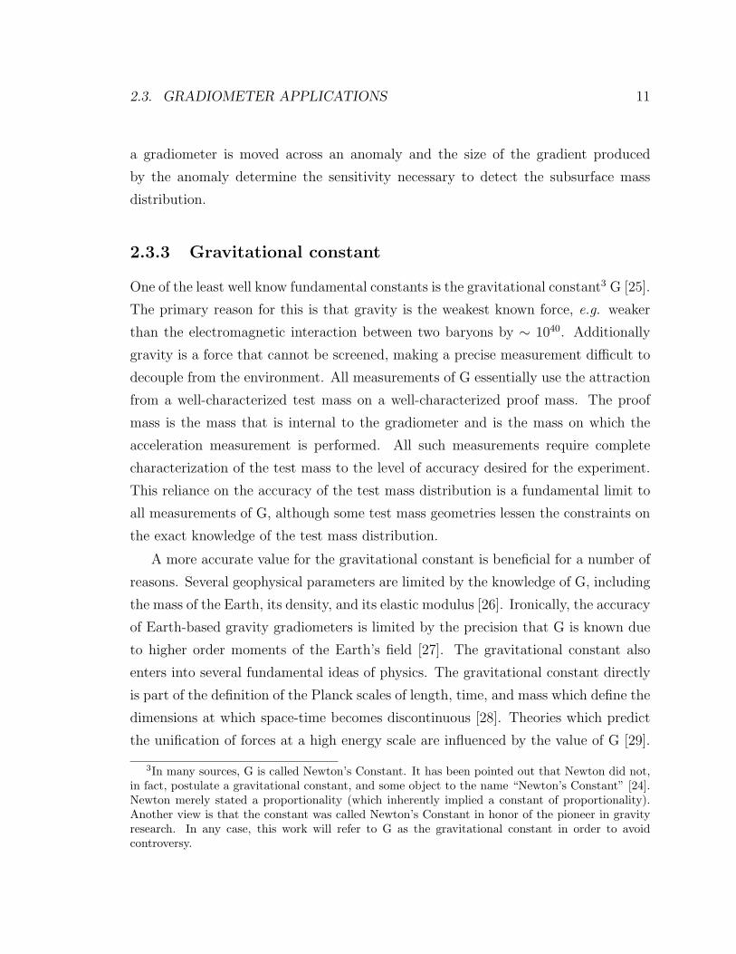
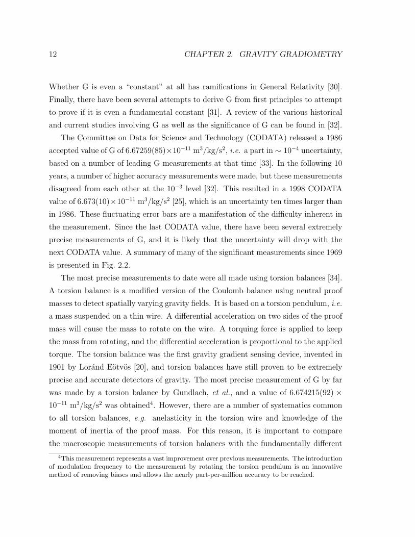
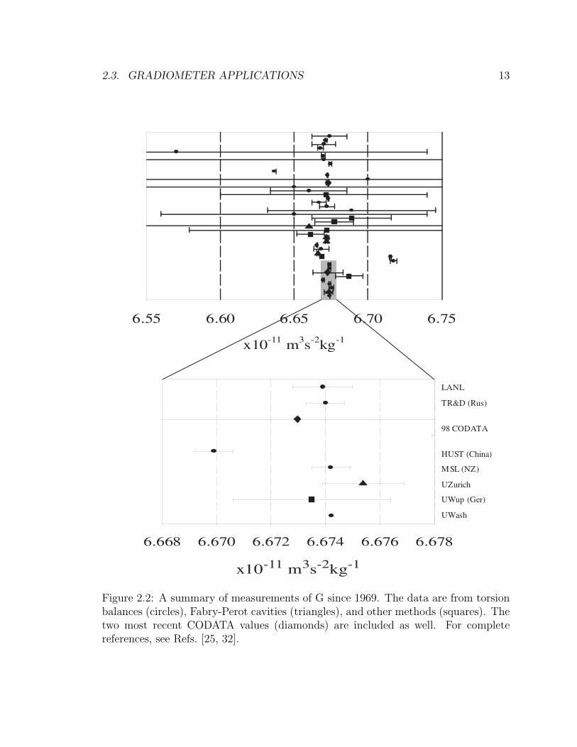
next CODATA value. A summary of many of the significant measurements since 1969
is presented in Fig. 2.2.
The most precise measurements to date were all made using torsion balances [34].
A torsion balance is a modified version of the Coulomb balance using neutral proof
masses to detect spatially varying gravity fields. It is based on a torsion pendulum, i.e.
a mass suspended on a thin wire. A differential acceleration on two sides of the proof
mass will cause the mass to rotate on the wire. A torquing force is applied to keep
the mass from rotating, and the differential acceleration is proportional to the applied
torque. The torsion balance was the first gravity gradient sensing device, invented in
1901 by Lorand Eotvos [20], and torsion balances have still proven to be extremely
precise and accurate detectors of gravity. The most precise measurement of G by far
was made by a torsion balance by Gundlach, et al., and a value of 6.674215(92) ×10−11 m3/kg/s2 was obtained4. However, there are a number of systematics common
to all torsion balances, e.g. anelasticity in the torsion wire and knowledge of the
moment of inertia of the proof mass. For this reason, it is important to compare
the macroscopic measurements of torsion balances with the fundamentally different
4This measurement represents a vast improvement over previous measurements. The introductionof modulation frequency to the measurement by rotating the torsion pendulum is an innovativemethod of removing biases and allows the nearly part-per-million accuracy to be reached.
2.3. GRADIOMETER APPLICATIONS 13
x10-11 m3s-2kg-1
6.668 6.670 6.672 6.674 6.676 6.678
x10-11 m3s-2kg-1
6.55 6.60 6.65 6.70 6.75
LANL
TR&D (Rus)
98 CODATA
HUST (China)
MSL (NZ)
UZurich
UWup (Ger)
UWash
Figure 2.2: A summary of measurements of G since 1969. The data are from torsionbalances (circles), Fabry-Perot cavities (triangles), and other methods (squares). Thetwo most recent CODATA values (diamonds) are included as well. For completereferences, see Refs. [25, 32].
14 CHAPTER 2. GRAVITY GRADIOMETRY
microscopic measurements of an atom interferometer.
2.3.4 Tests of General Relativity
Another interesting application of the gravity gradiometer described herein are tests
of General Relativity. There are string dilaton theories which predict the breakdown
of General Relativity [30]. This breakdown could manifest itself in a number of ways,
including time variation of G and thermal dependence of G. One class of tests seeks to
find violations of the inverse square law of gravity. A Yukawa type potential, αe−r/λ,
is predicted for wavelength λ less than 1 mm. Tests of the inverse square law at
short range could be performed using an atom interferometer gradiometer using tests
masses extremely close to the atoms.
Additionally, a breakdown of General Relativity can lead to violations of the
Equivalence Principle. The strong Equivalence Principle states that all laws of physics
hold in all reference frames, while the weak Equivalence Principle (WEP) states that
specifically the laws of gravity are true for all reference frames. In other words, the
WEP implies that inertial mass is equivalent to gravitational mass, i.e. that gravity
couples exactly to mass rather than some charge [35]. If there were any composition
dependent gravitational forces, then the WEP would be violated. This test is the
most sensitive test for General Relativity violations due to the predicted size of the
effects . There are predictions of composition dependent differences in gravitational
coupling at the 10−12g − 10−21g level [30], just outside of the current limits set by
torsion balances [36]. The gravity gradiometer presented herein is an ideal tool5 for
probing the composition dependence of gravity.
2.3.5 Fifth force experiments
An intriguing application for a gravity gradiometer is a search for “new physics.”
Included in this category are experiments seeking a fifth force. There are theories
which predict the existence of weakly interacting bosons called axions [37, 38, 39].
5This would not technically be a gravity gradiometer, but instead a dual-species differentialaccelerometer.
2.4. ALTERNATE GRADIOMETER TECHNOLOGIES 15
Axions might couple spin to matter through a scalar or a pseudo-scalar spin-gravity
coupling. Such a coupling to matter could produce a spin-dependent potential of the
form
U(r) α S · r(
1
λr+
1
r2
)e−r/λ, (2.2)
for a dipole-monopole coupling with range λ between two particles of distance r.
Using two coupled atom interferometer accelerometers as in the gravity gradiometer,
one could attempt to measure such a force or to put limits on the coupling strength.
Such a measurement would use one accelerometer as a local oscillator and would
compare the gravitational force experienced by atoms in a different spin state. If
such an axion coupling existed one might see a change in acceleration between atoms
in different spin states in the two interferometers.
2.4 Alternate gradiometer technologies
There are only a few different gradiometer technologies with both high precision and
accuracy. Part of the reason for the dearth of devices is that gravity gradients are
usually small and difficult to resolve. Additionally, vibrations enter the system as
a noise component if care is not taken with the measurements, particularly with
mechanical devices. This section briefly discusses three existing gradiometers. The
difference between absolute and relative gravity gradiometers is highlighted as well.
2.4.1 Mass-spring gradiometers
The state-of-the-art in mobile gradiometers is the Universal Gravity Module (UGM)
manufactured by Lockheed Martin, which is a device based on mechanical mass-
spring accelerometers [40]. The UGM consists of four (or eight) accelerometers on
a rotating platform. The accelerometers are devices which each capacitively mea-
sure the acceleration of a precisely machined proof-mass mounted on a spring. The
accelerometers are rotated to reject systematic drifts as well as to calibrate the de-
vice with the known centrifugal acceleration produced by rotation. The sensitivity
of this device ranges from 2 E/√
Hz to 20 E/√
Hz depending on the device baseline
16 CHAPTER 2. GRAVITY GRADIOMETRY
and the vibration environment, and the accuracy is limited to around 10 E [41]. This
device is currently employed for a variety of field applications including airborne oil
and mineral detection (BHP Falcon Project) [42], land-based underground structure
detection [43], and for navigational purposes aboard ballistic missile submarines [44].
2.4.2 Superconducting instruments
The leading device for short-term sensitivity is a superconducting gravity gradiome-
ter [45]. The superconducting gradiometer levitates two superconducting macroscopic
machined proof masses in a magnetic field using the Meissner Effect. The acceleration
of the two masses is detected using two superconducting quantum interference devices
(SQUIDs) which monitor the changing magnetic flux through current-carrying loops
as the proof masses change position, and the differential acceleration constitutes the
gradient signal. The SQUID loops are coupled so as to remove common-mode vibra-
tions of the two masses. The short-term sensitivity of this device is ∼ 0.1 E/√
Hz. The
superconducting gradiometer is primarily limited by its poor long-term performance.
The accuracy and stability are limited by severe 1/f noise coming from the tare ef-
fect in superconductors , as well as the susceptibility of the device to mechanical and
thermal shock [46, 47]. This drift, plus the necessity for large dewars of liquid helium,
make the superconducting gradiometer impractical for use on mobile platforms.
2.4.3 Falling cornercube gradiometer
There is an absolute accelerometer that measures the acceleration of a falling corner-
cube in one arm of a Michelson interferometer. The chirp rate of the optical fringes is
directly proportional to the acceleration experienced by the cornercube. By stacking
two such accelerometers on top of each other and using the differential chirp rate,
the gravity gradient is measured [48]. The currently demonstrated sensitivity of the
falling cornercube gravimeter is only 400 E/√
Hz however, and it remains to be seen if
the device can reject common-mode vibrations effectively. The stability of the falling
cornercube gradiometer should be excellent, as it references its calibration to the
wavelength of light used.
2.4. ALTERNATE GRADIOMETER TECHNOLOGIES 17
2.4.4 Absolute gradiometry
All of the gravity gradiometers developed previously, save the falling cornercube gra-
diometer, are gradiometers that require periodic calibration and suffer from drift6.
The atom interferometer gradiometer is the first demonstration of an absolute ac-
celerometer. The calibration is referenced to the wavelength of the light used in the
interferometer. The lasers are stabilized to a well known atomic transition in Cs, and
their frequency is stable over long times. There is a popular saying in the inertial force
sensing community that “all inertial force sensors are good thermometers,” due to
their sensitivity to temperature change. However, that proves not to be the case with
the light-pulse method of gradiometry, which is insensitive to drifts from environmen-
tal effects such as temperature and magnetic fields. The falling cornercube device also
references its calibration to the wavelength of the light used and should be stable as
well. An absolute accelerometer improves productivity by not requiring the return
to previous data sites for recalibration. Additionally, an absolute device is essential
for long-term use in inertial navigation systems and for scientific measurements with
long integration times.
6These gradiometers are called relative gradiometers.
Chapter 3
Laser Cooling and Trapping
The goal of this section is to describe the basic atom-photon interactions, called
atom optics, which are used throughout the experiments described in Chapter 5.
This chapter summarizes some basic tools of modern atom physics and describes the
results of the theoretical descriptions of them. There are a number of comprehensive
references that derive the results presented herein from first principles [49, 50], and
the reader is directed to them for complete derivations. The layout of the chapter is
as follows: first the structure of atoms is reviewed, and their basic behavior in optical
fields is summarized. Next is a description of optical forces on atoms and how they
are used to cool and confine atoms. Finally, a summary of the two-photon Raman
interactions used for the interferometer itself is given.
3.1 Atomic structure
In this dissertation, only alkali atoms will be considered, as they are the simplest to
deal with and most convenient. The atomic structure of all alkali atoms is a closed
inner shell plus the outermost electron in an S-shell. All alkali atoms are characterized
by two hyperfine ground state levels separated by a few gigahertz, corresponding to
a spin-flip of the valence electron, followed by a large spacing to the next allowed
transitions, the D1 and D2 lines in the optical regime. This level spacing makes alkali
18
3.2. TWO-LEVEL ATOMS 19
atoms particularly convenient to deal with, as they may effectively be treated as two-
level atoms in certain situations. The hyperfine structures only need be included in a
few specific calculations and are not necessary to derive many of the basic equations
for light forces on atoms.
Cesium (Cs) atoms are used exclusively in the experiments presented here. The
two hyperfine ground states of Cs are the 6S1/2 F = 3 and F = 4 levels, which
are separated by a 9.2 GHz microwave spin-flip transition. F is the total angular
momentum of the atom, F = J + I, where I = 7/2 is the nuclear spin. The electron
angular momentum is J = L + S; L and S are the spin-orbit coupling and the electron
spin respectively. It is this hyperfine splitting frequency that is the basis for the
System Internationale definition of the second. This frequency is a defined quantity,
and the Cs hyperfine transition is the basis for all primary time standards. The
D2 line to the 6P3/2 manifold is used for the cooling transition at 852 nm. The
excited manifold has 4 hyperfine states F′ = 2, 3, 4, and 5. The prime notation is
used to denote the excited manifold throughout this dissertation. In the presence
of a magnetic field, each hyperfine level is split further into 2F+1 Zeeman sublevels.
These sublevels are degenerate with no magnetic field. See Appendix A for the
detailed atomic structure of Cs, as well as for the physical properties of Cs.
3.2 Two-level atoms
The behavior of an ideal two-level atom in the presence of a single-frequency electric
field is presented here to demonstrate the phenomenon of Rabi flopping. The ground
and excited states are denoted |g〉 and |e〉 respectively. In the semi-classical approxi-
mation where the electric field is treated as a classical field, the Hamiltonian for such
an atom in the presence of the field is:
H = hωg|g〉〈g| + hωe|e〉〈e| + d · E. (3.1)
The first two terms represent the internal energy of the two states, hωg and hωe, while
the third term is the interaction between the electric dipole moment of the atom d
20 CHAPTER 3. LASER COOLING AND TRAPPING
and the electric field
E = Ecos(kx+ωt). (3.2)
The dipole interaction of the atom with the electric field gives an off-diagonal matrix
element of:
Ωr = −〈e|d · E|g〉h
, (3.3)
which is the Rabi frequency for oscillation between the ground and excited state for
resonant light, i.e. when ω = ωe − ωg [49]. Spontaneous emission has been neglected
here.
Using this Hamiltonian, the time-dependent Schrodinger Equation can be solved.
The full details of this solution are outside of the scope of this dissertation, and the
results will be summarized here. A complete description of Rabi flopping in a two-
level atom can be found in [51, 49]. By applying the rotating wave approximation,
shifting the arbitrary overall energy of the system, and transforming coordinates the
problem can be reduced to a simple solution. Using the initial condition that the
atom starts in the ground state |g〉, the probability of the atom being in the excited
state after being exposed to the laser field for time t is given by:
Pe(t) =1
2
[1 − Ω2
r
Ω′r2 cos(Ω
′rt)
], (3.4)
where Ω′r is the general expression for the Rabi frequency. Defining the detuning from
resonance as ∆ = ω − (ωe − ωg) , the generalized Rabi frequency is Ω′r =
√Ω2
r + ∆2.
A similar formula is true for finding the transition probability to the ground states if
the initial condition is |e〉. Additionally, the energy levels of the atom are shifted in
the presence of light field, called the AC Stark effect, by an amount:
UACg hΩ2
r
4∆. (3.5)
The AC Stark shift for the excited state is in the opposite direction as that for the
lower state: UACe = −UAC
g . Equation 3.5 is only valid in the limit of large detuning.
Following Equation 3.4, an atom in the ground or excited state illuminated with
3.3. OPTICAL FORCES 21
resonant light for a time t = π/Ωr will be transferred to the opposite state with
100% probability; such a pulse is called a π pulse. If the atom is illuminated for time
t = π/2Ωr, then the atom will be in an equal coherent superposition of the ground
and excited states, and this pulse is called a π/2 pulse. The terms π pulse and π/2
pulse are borrowed from nuclear magnetic resonance terminology and refer to the
pulse area. In practice, dephasing must be included due to effect like spontaneous
emission and various inhomogeneous broadening, which causes the amplitude of the
Rabi flopping to decrease.
An important concept to define is that of saturation of the atomic transition by
the electrical field. Because the atom has a finite natural lifetime1 τn, it can spend at
most half of the time in the excited state under incoherent scattering processes. This
means that after a point, the scattering rate ceases to increase as the intensity of the
driving field is increased. This phenomenon is called saturation, and the intensity at
which the probability of finding the atom in the excited state is 1/4 is defined as the
saturation intensity [52],
Isat = hck3Γn
2π. (3.6)
For the Cs F = 4 → F′ = 5 transition, Γn = 2π× 5.3 MHz, and Isat = 1.12 mW/cm2.
3.3 Optical forces
There are two main forces due to light acting on atoms: scattering forces and dipole
forces. Because the atoms are neutral, DC electrical forces are negligible unless ex-
tremely high electrical fields are present. The nature of each of the two primary forces
is discussed here.
3.3.1 Scattering force
The scattering force arises from the scattering of photons by an atom [49]. If a
photon from a resonant or near-resonant travelling-wave laser beam is absorbed by
the atom, through conservation of momentum, the atom receives a momentum kick
1The natural lifetime is the reciprocal of the natural linewidth, i.e. τn = 2π/Γn.
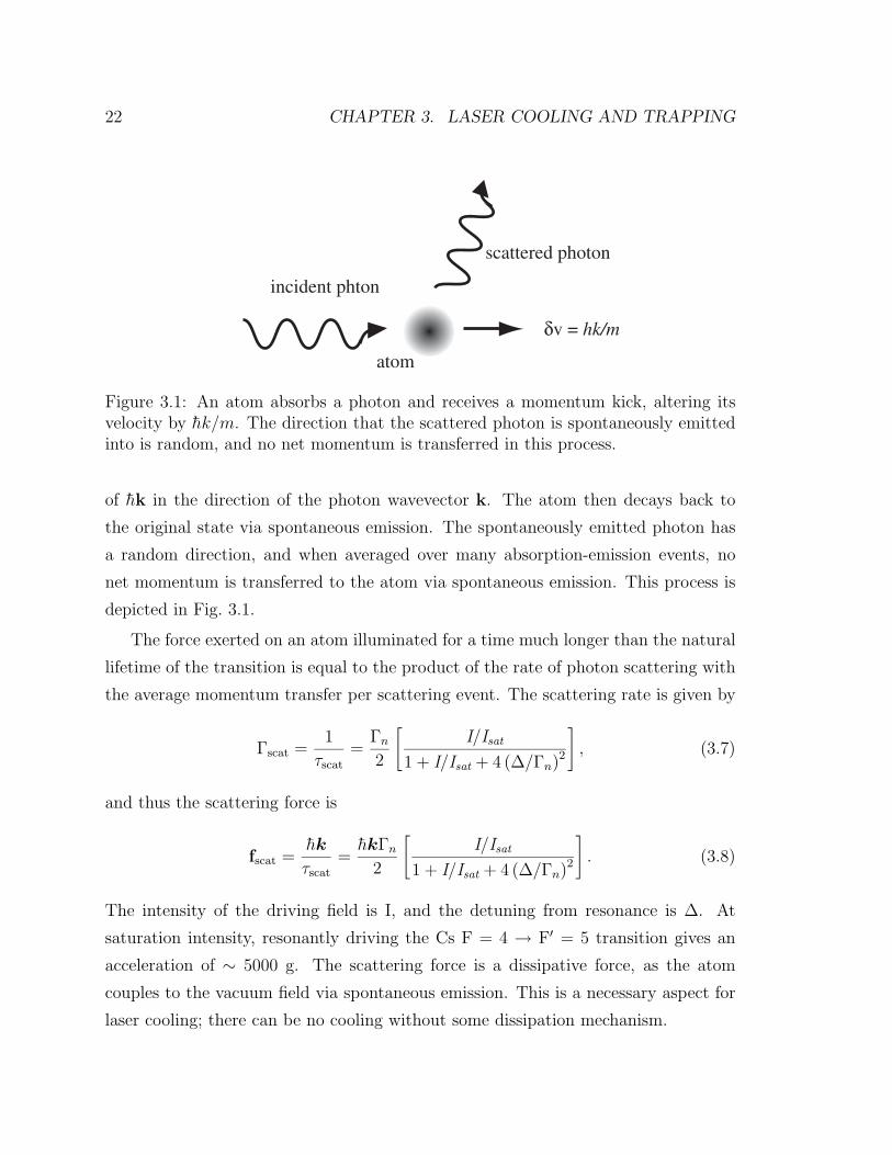
22 CHAPTER 3. LASER COOLING AND TRAPPING
incident phton
atom
scattered photon
δv = hk/m
Figure 3.1: An atom absorbs a photon and receives a momentum kick, altering itsvelocity by hk/m. The direction that the scattered photon is spontaneously emittedinto is random, and no net momentum is transferred in this process.
of hk in the direction of the photon wavevector k. The atom then decays back to
the original state via spontaneous emission. The spontaneously emitted photon has
a random direction, and when averaged over many absorption-emission events, no
net momentum is transferred to the atom via spontaneous emission. This process is
depicted in Fig. 3.1.
The force exerted on an atom illuminated for a time much longer than the natural
lifetime of the transition is equal to the product of the rate of photon scattering with
the average momentum transfer per scattering event. The scattering rate is given by
Γscat =1
τscat=
Γn
2
[I/Isat
1 + I/Isat + 4 (∆/Γn)2
], (3.7)
and thus the scattering force is
fscat =hk
τscat=
hkΓn
2
[I/Isat
1 + I/Isat + 4 (∆/Γn)2
]. (3.8)
The intensity of the driving field is I, and the detuning from resonance is ∆. At
saturation intensity, resonantly driving the Cs F = 4 → F′ = 5 transition gives an
acceleration of ∼ 5000 g. The scattering force is a dissipative force, as the atom
couples to the vacuum field via spontaneous emission. This is a necessary aspect for
laser cooling; there can be no cooling without some dissipation mechanism.
3.4. MAGNETIC FORCES 23
It should be noted that the F = 4 mF = 4 → F′ = 5 mF = 5 transition is a closed
transition for σ+ circularly polarized light (or F = 4 mF = -4 → F′ = 5 mF = -5
for σ−) due to selection rules. In the limit of perfectly polarized light, the atom will
cycle repeatedly through this transition. In practice, after many scattering events, the
atom will optically pump to the F = 3 state via a near-resonant transition from the
F = 4 mF = 4 → F′ = 5 mF = 4 due to a small component of linearly polarized light.
The atom can then spontaneously emit down to the F = 3 state, where it is unaffected
by the laser. Thus, in an experimental situation, the addition of a repumping beam
tuned to the F = 3 → F = 4 transition is necessary to repump the atoms out of the
dark state so they continue to scatter photons on the cycling transition.
3.3.2 Dipole force
Next consider the case of an atom in an oscillating electric field that is spatially
varying. The field shifts the energies of the atomic states by the AC-Stark potential
(see section 3.2). The spatially varying electric field causes the atom to experience a
force as given by the gradient of the potential,
fAC = −∇UAC Ω2r
∆ − hΓ2
n
2∆Isat
∇I(r). (3.9)
This means that an intensity gradient in a light field produces a force on an atom.
This force, called the dipole force, can be thought of in terms of the field polarizing the
atom and then exerting a force on the induced dipole. The dipole force can be used
to trap atoms at the focus of an intense beam [53]. However, for the purposes of the
experiments contained herein, the dipole force is an unwanted potential systematic
effect but is typically negligible for the intensity gradients involved.
3.4 Magnetic forces
An atom with a magnetic moment µ in a magnetic field B will experience an energy
shift that can be calculated by adding a magnetic field as a perturbation to the
Hamiltonian. The potential energy shift due to the magnetic field is Umag = −µ ·B.
24 CHAPTER 3. LASER COOLING AND TRAPPING
The magnetic moment is given by µ = mFgFµB, where mF is the quantum number
of the Zeeman sublevel, gF is the corresponding Lande g-factor, and µB is the Bohr
magneton. Calculations of the Lande g-factor can be found in many textbooks [49].
The g-factors of the two hyperfine ground states have opposite sign, meaning that the
Zeeman shift is opposite for the Zeeman sublevels of the F = 3 and F = 4 states. The
magnetic moment of ground state Cs atoms, in practical units, is mF× 350 kHz/G.
Atoms in the mF = 0 sublevel experience no first-order Zeeman energy shift. The
perturbative approximation used to calculate the the energy shift must be carried
out to second order in the magnetic field, and this energy shift is the second-order
Zeeman effect. For Cs atoms in the mF = 0, this shift is Umag = 2πhβB2, were β =
400 Hz/G2.
The force exerted by a magnetic field on an atom is given by the gradient of
the magnetic potential, F = −∇Umag. A static magnetic field exerts no force on
a neutral atom, but a spatial field gradient will exert a force on an atom with a
magnetic moment. Magnetic forces are used extensively in other atom trapping work
[54], particularly Bose-Einstein condensation (BEC) related work [55]. However, in
this experiment, they are only considered in the context of harmful systematic forces
acting on the atoms.
3.5 Laser cooling
3.5.1 Doppler cooling
The scattering force is a dissipative force, and it can be used to cool atoms, i.e. to
remove much of their kinetic energy2. Consider the situation depicted in Fig. 3.2, of
an atom travelling towards towards a laser beam that is red-detuned from a closed
cooling transition. The detuning seen by the atom will be modified by the Doppler
shift k · v due to the atom’s velocity v. The effective detuning for determining the
scattering rate and scattering force is ∆−k · v. There are two effects of the Doppler-
shifted detuning. The primary effect is that the laser will be Doppler-shifted towards
2The cooling discussed here damps the atom’s center of mass motion.
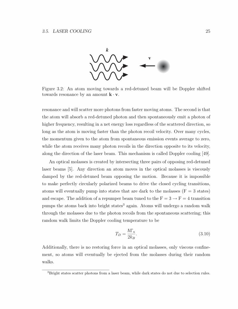
3.5. LASER COOLING 25
k
v
Figure 3.2: An atom moving towards a red-detuned beam will be Doppler shiftedtowards resonance by an amount k · v.
resonance and will scatter more photons from faster moving atoms. The second is that
the atom will absorb a red-detuned photon and then spontaneously emit a photon of
higher frequency, resulting in a net energy loss regardless of the scattered direction, so
long as the atom is moving faster than the photon recoil velocity. Over many cycles,
the momentum given to the atom from spontaneous emission events average to zero,
while the atom receives many photon recoils in the direction opposite to its velocity,
along the direction of the laser beam. This mechanism is called Doppler cooling [49].
An optical molasses is created by intersecting three pairs of opposing red-detuned
laser beams [5]. Any direction an atom moves in the optical molasses is viscously
damped by the red-detuned beam opposing the motion. Because it is impossible
to make perfectly circularly polarized beams to drive the closed cycling transitions,
atoms will eventually pump into states that are dark to the molasses (F = 3 states)
and escape. The addition of a repumper beam tuned to the F = 3 → F = 4 transition
pumps the atoms back into bright states3 again. Atoms will undergo a random walk
through the molasses due to the photon recoils from the spontaneous scattering; this
random walk limits the Doppler cooling temperature to be
TD =hΓn
2kB
. (3.10)
Additionally, there is no restoring force in an optical molasses, only viscous confine-
ment, so atoms will eventually be ejected from the molasses during their random
walks.
3Bright states scatter photons from a laser beam, while dark states do not due to selection rules.
26 CHAPTER 3. LASER COOLING AND TRAPPING
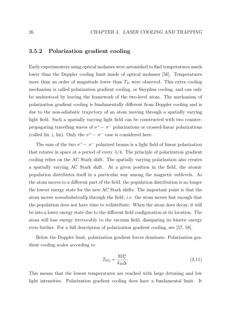
3.5.2 Polarization gradient cooling
Early experimenters using optical molasses were astonished to find temperatures much
lower than the Doppler cooling limit inside of optical molasses [56]. Temperatures
more than an order of magnitude lower than TD were observed. This extra cooling
mechanism is called polarization gradient cooling, or Sisyphus cooling, and can only
be understood by leaving the framework of the two-level atom. The mechanism of
polarization gradient cooling is fundamentally different from Doppler cooling and is
due to the non-adiabatic trajectory of an atom moving through a spatially varying
light field. Such a spatially varying light field can be constructed with two counter-
propagating travelling waves of σ+− σ− polarizations or crossed-linear polarizations
(called lin ⊥ lin). Only the σ+− σ− case is considered here.
The sum of the two σ+− σ− polarized beams is a light field of linear polarization
that rotates in space at a period of every λ/4. The principle of polarization gradient
cooling relies on the AC Stark shift. The spatially varying polarization also creates
a spatially varying AC Stark shift. At a given position in the field, the atomic
population distributes itself in a particular way among the magnetic sublevels. As
the atom moves to a different part of the field, the population distribution is no longer
the lowest energy state for the new AC Stark shifts. The important point is that the
atom moves nonadiabatically through the field, i.e. the atom moves fast enough that
the population does not have time to redistribute. When the atom does decay, it will
be into a lower energy state due to the different field configuration at its location. The
atom will lose energy irrevocably to the vacuum field, dissipating its kinetic energy
even further. For a full description of polarization gradient cooling, see [57, 58].
Below the Doppler limit, polarization gradient forces dominate. Polarization gra-
dient cooling scales according to
TPG =hΩ2
r
kB∆. (3.11)
This means that the lowest temperatures are reached with large detuning and low
light intensities. Polarization gradient cooling does have a fundamental limit. It
3.6. MAGNETO-OPTICAL TRAPPING 27
cannot cool below the limit of several photon recoils,
Trec ≡ (hk)2
2kBm(3.12)
where m is the mass of the atom. At these temperatures, the behavior of the atom
in the varying field, particularly in a three dimensional molasses, is complicated,
and a more involved treatment is necessary. Also, as with Doppler cooling, there
is no restoring force in polarization gradient cooling, and the atom will randomly
walk through the viscous confinement until it leaves the molasses region. Again,
a repumper is required with polarization gradient cooling to keep the atoms from
pumping into a dark state.
3.6 Magneto-optical trapping
Optical molasses is a an effective tool for dissipating the energy of atoms and cool-
ing them to ultra-cold temperatures. However, there is no restoring force to localize
the atoms and allow a large number to be collected. The optical Earnshaw theorem
states that it is not possible to trap atoms with light forces as long as the trapping
force is proportional to the intensity of the light [59]. This is easy to see: for any
given trapping volume, the optical energy entering the volume is the same as that
leaving the volume, thus there is no position with force vectors pointing inwards from
all directions. However because of the multiple atomic ground states, the addition
of a magnetic field gradient with a field minimum in the center of the intersecting
molasses laser beams provides an energy minimum and a restoring force that allows a
large number of atoms to be confined. This magnetic field is a spherical quadrupole
field created by two opposing coils of current-carrying wire in an anti-Helmholz con-
figuration. The spherical quadrupole has a field zero at the intersection of the beams
and a linearly increasing field directed radially outward.
To understand the trapping mechanism of a MOT, consider the one-dimensional
case depicted in Fig. 3.3. The magnetic field gradient changes the effective detuning
seen by an atom as it moves away from the field zero in the center, via the Zeeman
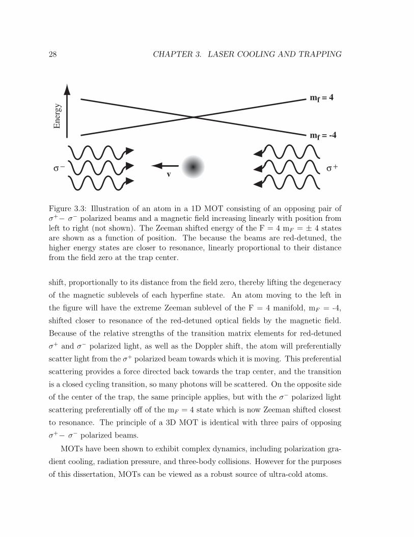
28 CHAPTER 3. LASER COOLING AND TRAPPINGE
nerg
y
v
mf = 4
mf = -4
σ − σ +
Figure 3.3: Illustration of an atom in a 1D MOT consisting of an opposing pair ofσ+− σ− polarized beams and a magnetic field increasing linearly with position fromleft to right (not shown). The Zeeman shifted energy of the F = 4 mF = ± 4 statesare shown as a function of position. The because the beams are red-detuned, thehigher energy states are closer to resonance, linearly proportional to their distancefrom the field zero at the trap center.
shift, proportionally to its distance from the field zero, thereby lifting the degeneracy
of the magnetic sublevels of each hyperfine state. An atom moving to the left in
the figure will have the extreme Zeeman sublevel of the F = 4 manifold, mF = -4,
shifted closer to resonance of the red-detuned optical fields by the magnetic field.
Because of the relative strengths of the transition matrix elements for red-detuned
σ+ and σ− polarized light, as well as the Doppler shift, the atom will preferentially
scatter light from the σ+ polarized beam towards which it is moving. This preferential
scattering provides a force directed back towards the trap center, and the transition
is a closed cycling transition, so many photons will be scattered. On the opposite side
of the center of the trap, the same principle applies, but with the σ− polarized light
scattering preferentially off of the mF = 4 state which is now Zeeman shifted closest
to resonance. The principle of a 3D MOT is identical with three pairs of opposing
σ+− σ− polarized beams.
MOTs have been shown to exhibit complex dynamics, including polarization gra-
dient cooling, radiation pressure, and three-body collisions. However for the purposes
of this dissertation, MOTs can be viewed as a robust source of ultra-cold atoms.
3.6. MAGNETO-OPTICAL TRAPPING 29
3.6.1 Trap loading
Atoms can be loaded into a MOT from a variety of sources. The simplest source is
a thermal vapor [6]. A low pressure thermal vapor of atoms is introduced into the
vacuum chamber. Atoms which enter the intersection of the trapping beams will be
captured if their velocity is low enough. In practice, this amounts to trapping only the
slow-atom tail of the Maxwell velocity distribution, which is sufficient for obtaining
large numbers. In order to build up a large enough vapor pressure, the walls of the
vacuum chamber must be coated with a mono-layer of atoms in order for a vapor
cell to be established. Otherwise, the clean vacuum chamber walls themselves are an
effective pump for alkali atoms. Other loading sources include beam loading, filament
loading, and loading from other pre-loaded atom traps. Vapor cell loading is used
exclusively in this dissertation.
The loading rate is primarily determined by only a few physical parameters re-
lating to the trapping laser beams and the partial pressures of gases in the vacuum
chamber [60]. The steady-state number of trapped atoms occurs at the point where
the loading rate is balanced by the loss rate. The loading rate is determined by the
density n and most probably velocity u of the Cs atoms as well as the parameters
of the trapping lasers, i.e. the diameter d of the beams, the scattering rate for the
cooling transition, and the recoil velocity vrec of the atoms after a scattering event:
Γload =4nd4Γ2
scatv2rec
u3. (3.13)
The primary loss mechanism in MOTs is collisions with untrapped atoms in the
background gas. In a vapor cell MOT, these atoms are usually untrapped Cs atoms
if the pressure of other background gases is sufficiently low. The collision rate is:
Γcol nbackσu, (3.14)
where nback is the total density of all background gases including the Cs vapor, and
σ is the cross section for a background collision that ejects an atom from the trap.
30 CHAPTER 3. LASER COOLING AND TRAPPING
The steady-state trap population is then given by:
Nss =Γload
Γcol
=4d4Γ2
scatv2rec
σu4
(n
nback
). (3.15)
In the limit where the Cs vapor pressure is small, the steady-state population is
linearly dependent on the Cs pressure. The opposite limit is rather surprising: if
the Cs vapor pressure is much larger than that of the other background gases, the
total steady-state population is independent of the Cs pressure. This limit has larger
steady-state populations as well. In practice this experiment is operated in the middle
region where both the Cs vapor pressure and the background gas pressure need to be
taken into consideration. There is also an upper bound on the Cs vapor pressure. If
the background collision rate is faster than the time it takes to slow and trap a Cs
atom, then a MOT is not possible. Experimentally, this high pressure cut-off occurs
around 10−7 torr. There is also a interferometric phase shift produced from collisions
with other atoms, but this effect is dominated by collisions with cold atoms instead
of the thermal background atoms at the standard operating pressures. Also of note
is the large dependence on the size of the trapping beams. This size is the most
important parameter to collect large numbers of atoms in a MOT.
3.6.2 Atomic fountains
Often experiments using trapped atoms require long interrogation times, particularly
interferometers. If all the trapping fields are turned off, the laser-cooled atoms begin
accelerating under the influence of gravity. Gravity causes the atoms to accelerate
away from the experiment region of the vacuum chamber and become inaccessible to
manipulation and detection after only tens of milliseconds. However, if the atoms are
accelerated upwards before being released from the optical molasses they will follow
ballistic trajectories and return to the initial trapping region after a time as long a
second. This allows for increased interaction time which is critical for the performance
of highly sensitive interferometers. Such optically induced ballistic trajectories are
called atomic fountains, and were first demonstrated in 1989 by Chu and Kasevich
[61].
3.7. TWO-PHOTON STIMULATED RAMAN TRANSITIONS 31
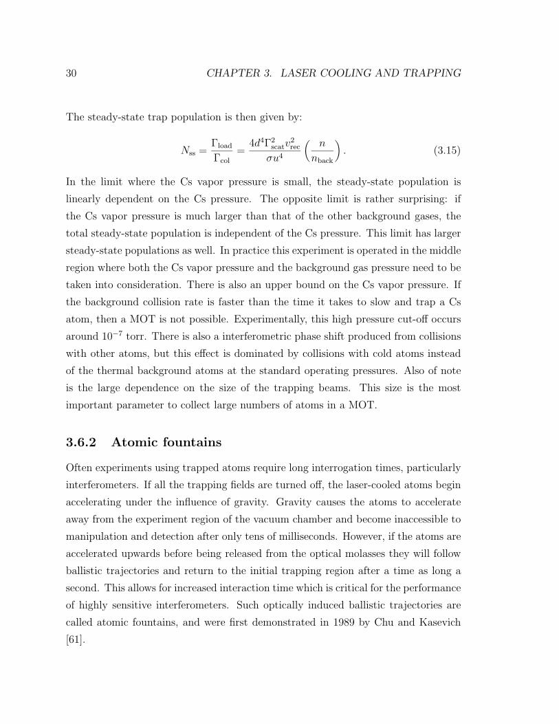
The atomic fountain is implemented as follows. After loading a MOT, the mag-
netic field is turned off, leaving the atoms confined in an optical molasses. If the
downward pointing beams are detuned further from resonance than the upward point-
ing beams, the downward pointing beams will transfer less momentum to the atoms
than the upward pointing beams, providing a net force upwards. This configuration
results in a molasses moving upwards at a velocity given by the frequency difference
between the upward and downward pointing beams. For the configuration shown in
Fig. 3.4a the velocity of the molasses is simply
v =δω
k(3.16)
for a frequency difference δω and an average wavevector k. This launching config-
uration has been shown to heat the atoms and is more difficult to work with than
the following scheme. The (1,1,1) MOT configuration4 shown in Fig. 3.4b does not
significantly heat the atoms and is more robust to beam pointing instabilities. The
velocity in this case is
v =δω
k sin(
π3
) . (3.17)
The extra factor in the denominator is a geometric factor accounting for the projection
of momenta onto the vertical axis. After the atoms are in the moving molasses, the
launching light can be shut off, and the atoms will follow ballistic trajectories under
the influence of gravity with the initial velocity of the moving molasses. Using such
an atomic fountain is an effective tool to dramatically increase interaction times for
cold atom experiments which require long interrogation times.
3.7 Two-photon stimulated Raman transitions
Raman transitions are a type of inelastic scattering of a light field by an atom.
Through the process, the atom gains or loses energy, and thus has its momentum
4The notation (1,0,0) and (1,1,1) is taken from crystal geometries in condensed matter physics.
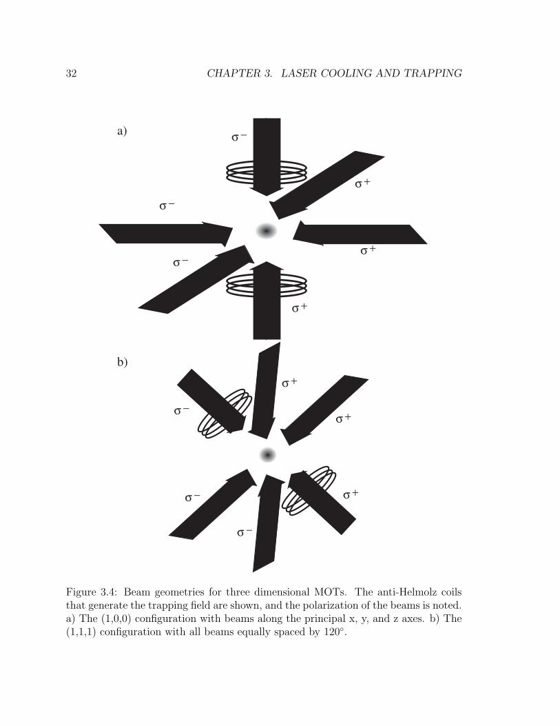
32 CHAPTER 3. LASER COOLING AND TRAPPING
σ −
σ −
σ −
σ −
σ −
σ −
σ +
σ +
σ +
σ +
σ +
σ +
a)
b)
Figure 3.4: Beam geometries for three dimensional MOTs. The anti-Helmolz coilsthat generate the trapping field are shown, and the polarization of the beams is noted.a) The (1,0,0) configuration with beams along the principal x, y, and z axes. b) The(1,1,1) configuration with all beams equally spaced by 120.
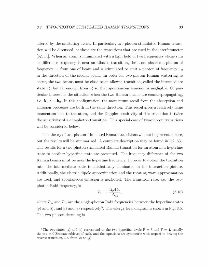
3.7. TWO-PHOTON STIMULATED RAMAN TRANSITIONS 33
altered by the scattering event. In particular, two-photon stimulated Raman transi-
tion will be discussed, as these are the transitions that are used in the interferometer
[62, 14]. When an atom is illuminated with a light field of two frequencies whose sum
or difference frequency is near an allowed transition, the atom absorbs a photon of
frequency ω1 from one of beam and is stimulated to emit a photon of frequency ω2
in the direction of the second beam. In order for two-photon Raman scattering to
occur, the two beams must be close to an allowed transition, called the intermediate
state |i〉, but far enough from |i〉 so that spontaneous emission is negligible. Of par-
ticular interest is the situation when the two Raman beams are counterpropagating,
i.e. k1 −k2. In this configuration, the momentum recoil from the absorption and
emission processes are both in the same direction. This recoil gives a relatively large
momentum kick to the atom, and the Doppler sensitivity of this transition is twice
the sensitivity of a one-photon transition. This special case of two-photon transitions
will be considered below.
The theory of two-photon stimulated Raman transitions will not be presented here,
but the results will be summarized. A complete description may be found in [52, 63].
The results for a two-photon stimulated Raman transition for an atom in a hyperfine
state to another hyperfine state are presented. The frequency difference of the two
Raman beams must be near the hyperfine frequency. In order to obtain the transition
rate, the intermediate state is adiabatically eliminated in the interaction picture.
Additionally, the electric dipole approximation and the rotating wave approximation
are used, and spontaneous emission is neglected. The transition rate, i.e. the two-
photon Rabi frequency, is
Ωeff =ΩgiΩie
∆eg
, (3.18)
where Ωgi and Ωie are the single-photon Rabi frequencies between the hyperfine states
|g〉 and |i〉, and |i〉 and |e〉 respectively5. The energy level diagram is shown in Fig. 3.5.
The two-photon detuning is
5The two states |g〉 and |e〉 correspond to the two hyperfine levels F = 3 and F = 4, usuallythe mF = 0 Zeeman sublevel of each, and the equations are symmetric with respect to driving thereverse transition, i.e. from |e〉 to |g〉.

34 CHAPTER 3. LASER COOLING AND TRAPPING
|i ⟩
|g ⟩
|e ⟩
k1 k2
∆
ωhf
∆eg
Figure 3.5: Energy level diagram for Raman transitions. The detuning ∆ of thevirtual state is large compared to the two photon Rabi frequency, but small comparedto the energy spacing between it and levels |e〉 and |g〉 (which is an optical transitionin this experiment). The two-photon detuning ∆eg is shown, and is usually set tozero for driving transitions.
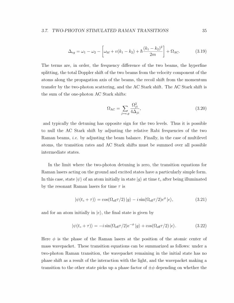
3.7. TWO-PHOTON STIMULATED RAMAN TRANSITIONS 35
∆eg = ω1 − ω2 −[ωhf + v(k1 − k2) + h
(k1 − k2)2
2m
]+ ΩAC. (3.19)
The terms are, in order, the frequency difference of the two beams, the hyperfine
splitting, the total Doppler shift of the two beams from the velocity component of the
atoms along the propagation axis of the beams, the recoil shift from the momentum
transfer by the two-photon scattering, and the AC Stark shift. The AC Stark shift is
the sum of the one-photon AC Stark shifts:
ΩAC =∑
j=e,g
Ω2ji
4∆ji
, (3.20)
and typically the detuning has opposite sign for the two levels. Thus it is possible
to null the AC Stark shift by adjusting the relative Rabi frequencies of the two
Raman beams, i.e. by adjusting the beam balance. Finally, in the case of multilevel
atoms, the transition rates and AC Stark shifts must be summed over all possible
intermediate states.
In the limit where the two-photon detuning is zero, the transition equations for
Raman lasers acting on the ground and excited states have a particularly simple form.
In this case, state |ψ〉 of an atom initially in state |g〉 at time t after being illuminated
by the resonant Raman lasers for time τ is
|ψ(t + τ)〉 = cos(Ωeffτ/2) |g〉 − i sin(Ωeffτ/2)eφ |e〉, (3.21)
and for an atom initially in |e〉, the final state is given by
|ψ(t + τ)〉 = −i sin(Ωeffτ/2)e−φ |g〉 + cos(Ωeffτ/2) |e〉. (3.22)
Here φ is the phase of the Raman lasers at the position of the atomic center of
mass wavepacket. These transition equations can be summarized as follows: under a
two-photon Raman transition, the wavepacket remaining in the initial state has no
phase shift as a result of the interaction with the light, and the wavepacket making a
transition to the other state picks up a phase factor of ±φ depending on whether the
36 CHAPTER 3. LASER COOLING AND TRAPPING
atom was initially in the ground or excited state.
To summarize, stimulated, two-photon Raman transitions are useful tools for co-
herent manipulation of atoms. They transfer relatively large momenta to atoms and
have high Doppler sensitivity. Also, the frequency difference of the two beams is the
important quantity in the detuning of the lasers. This means that each laser does not
have to be stabilized to a part in 1015, but rather that their frequency difference has
to be stabilized to the same sub-Hertz level, or only a part in 1010. Finally, there are
simple transition rules governing the atomic phase under a Raman transitions that
make interferometer phase calculations straightforward.
3.8 Atom detection
It is essential to be able to read out the populations of the atomic states following
an experiment. In a precision measurement this must be done as cleanly as possible.
The detection must be state-selective as well in the case of two state atom interfer-
ometers. There are several types of detection available for neutral atoms with low
energies: fluorescence, absorption, and dispersion detection. These detection methods
are described briefly here and are discussed in depth in section 5.7.
Fluorescent detection is the easiest detection scheme to implement. The atoms are
illuminated with light that is resonant or nearly-resonant to an optical transition. The
photons spontaneously emitted from the atoms are detected on some imaging device,
such as a photodiode, photo-multiplier tube, or a charge-coupled device camera. If
the light is tuned to a closed transition, i.e. the cooling transition for an atom in
the F = 4 state, then the atom will scatter many photons before the atom optically
pumps to a dark state via off-resonant excitations (the F = 3 state here). Under
typical experimental conditions for Cs atoms in the F = 4 state, using light tuned to
the cooling transition at I = Isat, about 1000 photons will be scattered from each atom
before it pumps into the F = 3 state and goes dark to the detection light. Atoms in
the F = 3 state usually must be first pumped into the F = 4 state with a repumper
before detection, as there is no closed transition from the F = 3 manifold.
Fluorescent detection scatters light into a solid angle of 4π steradian. If the
3.9. EXPERIMENT SYNOPSIS 37
solid angle that the detector (or the collection lens before the detector) subtends
is significantly smaller than this, then very few photons per atom will be detected.
These smaller signal levels can lead to problems with counting statistics and can be
limited by technical noise as well. To overcome this solid angle problem, which is often
limited by the fundamental geometry of the experiment, absorption detection may
be used. The principle of absorption detection is similar to fluorescence detection,
except that the intensity of the scattering beam is detected with a photodiode, and
the photons not scattered by the atoms are detected. In this way, essentially all
the scattered photons are detected (or more precisely the absence of the photons is
detected), and the detection statistics are improved, provided the shot noise from the
unabsorbed portion of the light is not too large.
The final detection method employed with ultra-cold atoms is a dispersive mea-
surement. This is similar to absorption except the complex part of the atoms’ index
of refraction is measured here, whereas absorption measures the real part. The dis-
persion of an off-resonant detection beam as it passes through the atoms is measured
by heterodyning it with a local oscillator. This method is primarily useful for dense
clouds of atoms with large refractive indices, such as BECs. For the relatively diffuse
clouds produced by atoms at MOT temperatures at low densities following atomic
fountains, this method produces small signals and is not suitable.
3.9 Experiment synopsis
Having described some of the basic tools of atom optics, it is now possible to describe
the gravity gradiometer experiment in more detail. First Cs atoms are cooled and
trapped from a thermal vapor at two spatially separated regions in two MOTs. Each
ensemble of cold atoms is then launched in an atomic fountain in a specially prepared
hyperfine state. During the fountain, the atoms are interrogated with a three pulse
π/2 − π − π/2 interferometer sequence consisting of stimulated two-photon Raman
transitions. The phase of the atoms following the interferometer is determined by
the atoms’ interaction with the interferometer laser fields as well as the free evolution
of the atom, both of which are influenced by the presence of gravity. Following the
38 CHAPTER 3. LASER COOLING AND TRAPPING
interferometer, the relative populations of the two hyperfine states are read out using a
sensitive detection scheme. The difference between the gravitationally induced phases
from the two ensembles of atoms is directly proportional to the gravity gradient.
Chapter 4
Atom Interferometry
It may seem obvious that the interferometer phase shift of an atom falling in a grav-
itational field is
φ = keff · gT 2, (4.1)
to first-order. After all, this phase is simply the total distance travelled by the atom
experiencing acceleration g in time T , gT 2/2, divided by the effective wavelength
of the interferometer light used to “measure the distance,” 1/keff = λ/2. It is not
obvious how this is related to an interferometer however. This chapter attempts to
explain the interferometer phase shift and to present several different techniques for
obtaining precise phase shift calculations. First an intuitive heuristic description is
given, followed by a discussion of the total interferometer phase. Each term of the
interferometer phase is discussed and calculated. Particular detail is given to the
phase shift from the free propagation of the atoms between interferometer pulses.
The application of these methods to nonuniform acceleration fields is described. The
limits and merits of each case are discussed. The fundamental assumptions made in
the starting point for these phase calculations are considered. Finally, the application
of these results to gravity gradiometers is discussed.
39
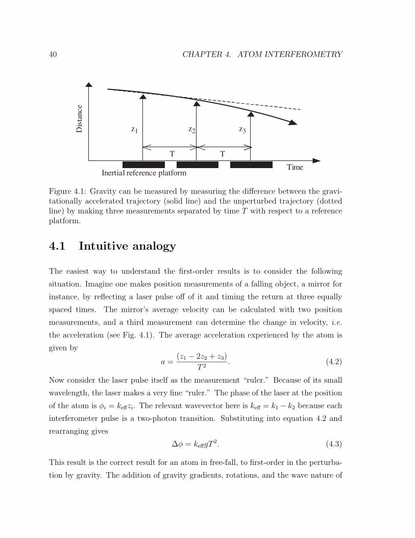
40 CHAPTER 4. ATOM INTERFEROMETRY
Inertial reference platform
z1
T T
Time
Dis
tanc
e
z2 z3
Figure 4.1: Gravity can be measured by measuring the difference between the gravi-tationally accelerated trajectory (solid line) and the unperturbed trajectory (dottedline) by making three measurements separated by time T with respect to a referenceplatform.
4.1 Intuitive analogy
The easiest way to understand the first-order results is to consider the following
situation. Imagine one makes position measurements of a falling object, a mirror for
instance, by reflecting a laser pulse off of it and timing the return at three equally
spaced times. The mirror’s average velocity can be calculated with two position
measurements, and a third measurement can determine the change in velocity, i.e.
the acceleration (see Fig. 4.1). The average acceleration experienced by the atom is
given by
a =(z1 − 2z2 + z3)
T 2. (4.2)
Now consider the laser pulse itself as the measurement “ruler.” Because of its small
wavelength, the laser makes a very fine “ruler.” The phase of the laser at the position
of the atom is φi = keffzi. The relevant wavevector here is keff = k1 − k2 because each
interferometer pulse is a two-photon transition. Substituting into equation 4.2 and
rearranging gives
∆φ = keffgT2. (4.3)
This result is the correct result for an atom in free-fall, to first-order in the perturba-
tion by gravity. The addition of gravity gradients, rotations, and the wave nature of
4.2. INTERFEROMETER DESCRIPTION 41
the atom complicates the situation. This gravitational phase shift is around 106 rad
for typical experimental parameters in the presence of Earth’s gravity. The goal of
gradiometry is the detect differences that are typically 10−8g (0.01 rad) or much less
between two such gravimeters.
4.2 Interferometer description
The interferometer is formed by three pulses, each driving a velocity-sensitive, two-
photon, stimulated Raman transition between two long-lived hyperfine ground states
[14]. The pulse sequence is a π/2−π−π/2 pulse sequence and is a modification of the
Ramsey separated oscillatory field sequence1 π/2 − π/2 [8]. With the atom initially
in the ground state |g〉 the first π/2 pulses puts the atom in a coherent superposition
between the ground and excited states. This pulse acts as a beamsplitter by trans-
ferring momentum hkeff to the wavepacket that makes the transition to the excited
state. In this interferometer there is a one-to-one correlation between internal states
and momentum states of the atom. The two wavepackets propagate freely, only influ-
enced by inertial forces, while drifting apart with relative momentum hkeff. At a time
T later, the second pulse, a π pulse, is applied. This pulse interchanges the ground
and excited states, while reversing their relative momenta. The two wavepackets then
drift back towards each other for time T . Finally, at time 2T after the first π/2 pulse,
the final π/2 pulse recombines the two wavepackets, interfering them. This sequence
is depicted in a recoil diagram in Fig. 4.2. During each pulse, the phase of the op-
tical field at the position of the atoms is imprinted on the internal state probability
amplitude of the atoms, as described in section 3.7. The probability of finding the
atom in a particular state following the interferometer depends on the relative phase
accrued by the two interfering wavepackets during the interferometer, and this phase
depends on the inertial forces experienced by the atom [16].
1The modification is necessary because the Raman sequence transfers non-negligible momentumto the atom, and the extra π pulse ensures the two wavepackets overlap at the end of the interfer-ometer.
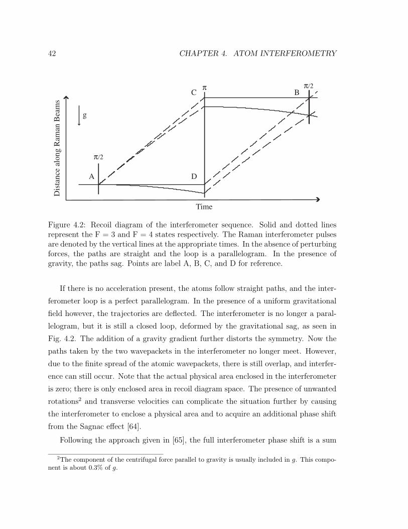
42 CHAPTER 4. ATOM INTERFEROMETRY
Time
Dis
tanc
e al
ong
Ram
an B
eam
s
π/2
π π/2
g
A
BC
D
Figure 4.2: Recoil diagram of the interferometer sequence. Solid and dotted linesrepresent the F = 3 and F = 4 states respectively. The Raman interferometer pulsesare denoted by the vertical lines at the appropriate times. In the absence of perturbingforces, the paths are straight and the loop is a parallelogram. In the presence ofgravity, the paths sag. Points are label A, B, C, and D for reference.
If there is no acceleration present, the atoms follow straight paths, and the inter-
ferometer loop is a perfect parallelogram. In the presence of a uniform gravitational
field however, the trajectories are deflected. The interferometer is no longer a paral-
lelogram, but it is still a closed loop, deformed by the gravitational sag, as seen in
Fig. 4.2. The addition of a gravity gradient further distorts the symmetry. Now the
paths taken by the two wavepackets in the interferometer no longer meet. However,
due to the finite spread of the atomic wavepackets, there is still overlap, and interfer-
ence can still occur. Note that the actual physical area enclosed in the interferometer
is zero; there is only enclosed area in recoil diagram space. The presence of unwanted
rotations2 and transverse velocities can complicate the situation further by causing
the interferometer to enclose a physical area and to acquire an additional phase shift
from the Sagnac effect [64].
Following the approach given in [65], the full interferometer phase shift is a sum
2The component of the centrifugal force parallel to gravity is usually included in g. This compo-nent is about 0.3% of g.
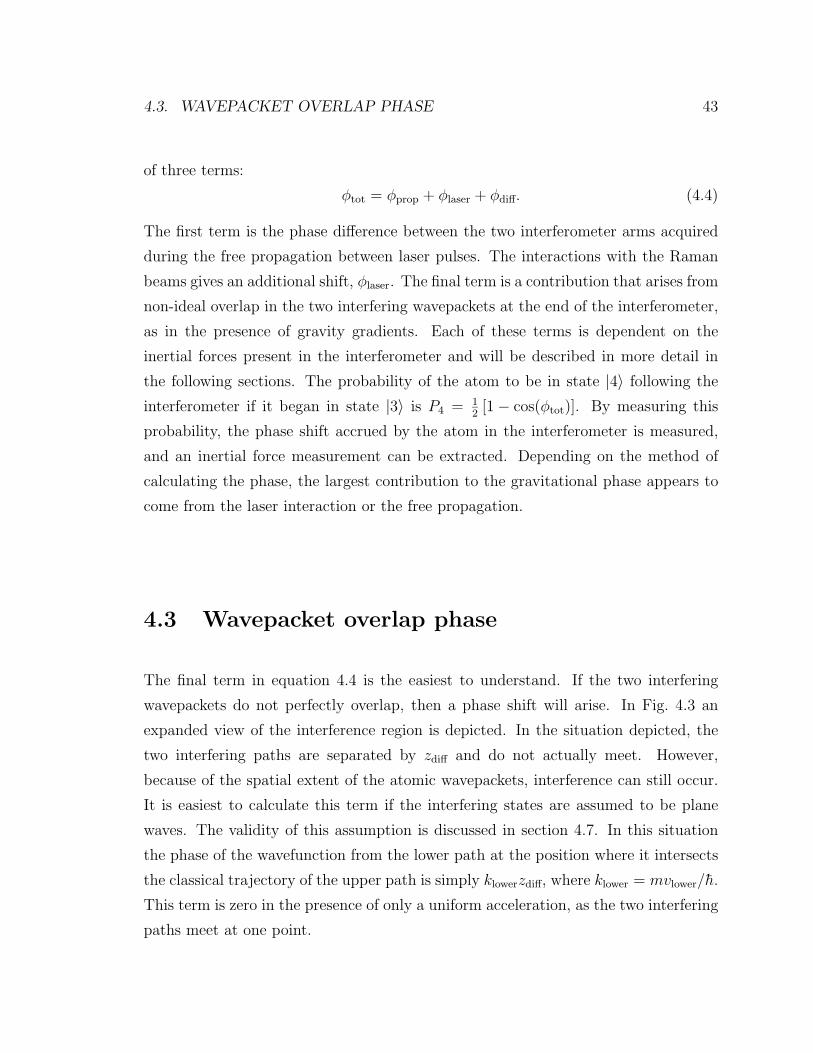
4.3. WAVEPACKET OVERLAP PHASE 43
of three terms:
φtot = φprop + φlaser + φdiff. (4.4)
The first term is the phase difference between the two interferometer arms acquired
during the free propagation between laser pulses. The interactions with the Raman
beams gives an additional shift, φlaser. The final term is a contribution that arises from
non-ideal overlap in the two interfering wavepackets at the end of the interferometer,
as in the presence of gravity gradients. Each of these terms is dependent on the
inertial forces present in the interferometer and will be described in more detail in
the following sections. The probability of the atom to be in state |4〉 following the
interferometer if it began in state |3〉 is P4 = 12[1 − cos(φtot)]. By measuring this
probability, the phase shift accrued by the atom in the interferometer is measured,
and an inertial force measurement can be extracted. Depending on the method of
calculating the phase, the largest contribution to the gravitational phase appears to
come from the laser interaction or the free propagation.
4.3 Wavepacket overlap phase
The final term in equation 4.4 is the easiest to understand. If the two interfering
wavepackets do not perfectly overlap, then a phase shift will arise. In Fig. 4.3 an
expanded view of the interference region is depicted. In the situation depicted, the
two interfering paths are separated by zdiff and do not actually meet. However,
because of the spatial extent of the atomic wavepackets, interference can still occur.
It is easiest to calculate this term if the interfering states are assumed to be plane
waves. The validity of this assumption is discussed in section 4.7. In this situation
the phase of the wavefunction from the lower path at the position where it intersects
the classical trajectory of the upper path is simply klowerzdiff, where klower = mvlower/h.
This term is zero in the presence of only a uniform acceleration, as the two interfering
paths meet at one point.
44 CHAPTER 4. ATOM INTERFEROMETRYD
ista
nce
alon
g R
aman
Bea
ms
Time
g π/2
zdiff
Figure 4.3: Recoil diagram showing the mismatch in paths zdiff after the interferometerin the presence of gravity gradients. Interference can still occur if zdiff is less than thecoherence length of the atomic wavepacket.
4.4 Laser phase
The contribution to the total phase in equation 4.4 from the laser-atom interactions
φlaser can be calculated from the rules for two-photon Raman transitions presented in
section 3.7. The total laser phase is the laser phase imparted to the top path minus
the phase imparted to the lower path. Assuming the atom initially starts in state |3〉,following the transition rules given in Eqs. 3.21 and 3.22 this phase is:
φlaser = φ1 − 2φ2 + φ3. (4.5)
The phases φi are the phases imprinted on the atom by the ith Raman pulses. For an
atom following a classical path in a uniform gravity field, each phase at time ti and
atomic center of mass position xi is:
φi = ωiti − keff·xi + φi = ωiti − 1
2keffgt
2i + φ
i . (4.6)
Here the trajectories and Raman beams are assumed to be parallel with g, ωi is the
frequency of the Raman lasers at the time of the ith pulse, and φi is the arbitrary
4.4. LASER PHASE 45
phase of the laser. Recall that keff = k1 − k2 2k1. Only the case of
t1 = 0
t2 = T (4.7)
t3 = 2T
is considered, i.e. an interferometer with pulses spaced equally by time T .
4.4.1 Frequency term
For a constant frequency ω the frequency terms in equation 4.6 cancel and equation 4.5
reduces to
φlaser = keffgT2 + ∆φ, (4.8)
where ∆φ = φ1−2φ
2+φ3. However, for typical experimental interaction times of 100
ms or more, the Doppler shift due to gravity is keffgT ∼ 1 MHz. This Doppler shift
is much larger than the typical two-photon Rabi frequency Ωeff ∼ 30 kHz. Thus if
the laser frequency is kept constant throughout the interferometer, the atoms quickly
Doppler shift out of resonance with the beams due to the acceleration of gravity.
Typically, to counteract this effect the frequency of the laser is linearly chirped at a
rate δω equal to the gravitational Doppler shift:
ω(t) = ω − δω(t− t1) = ω − keffg(t− t1). (4.9)
The frequency term then exactly offsets the gravitational phase term in equation 4.6
and φlaser = ∆φ. In other words, the frequency is chirped at exactly the same rate
as the atom is accelerating, and the atom sees wavefronts of constant phase in the
falling frame. The gravity information is contained in the precise knowledge of the
frequency chirp3. In theoretical discussions, including the rest of this chapter, this
frequency chirp is typically ignored as an experimental detail.
3For the given transitions in Cs, the chirp rate is 23 MHz/s. Frequency chirps of this rateare routine to generate precisely. Additionally, for a gradient measurement, the frequency chirp iscommon to both accelerometers and is not an issue.
46 CHAPTER 4. ATOM INTERFEROMETRY
4.4.2 Initial phase
The third term in φlaser, the initial laser phase, is now examined. If the Raman lasers
are temporally coherent across the time of the interferometer, then the initial phase
for each pulse will be the same, and ∆φ = 0. The temporal coherence length for a
single laser is 1/∆ν, the reciprocal of the linewidth, and is typically ∼ 1/300 kHz for
a commercial diode laser. However, for a two-photon process, what is important is
the temporal coherence of the difference frequency, not the absolute frequency. This
difference frequency is locked to a microwave source at the hyperfine frequency which
has a sub-Hertz linewidth. This linewidth translates into an effective coherence time
of significantly greater than a second, which is the timescale for the interferometer
pulses. If all frequency synthesizers used to generate the Raman pulses have typical
coherences and the pulses themselves are generated in a phase-continuous way, i.e. as
from a continuously chirped sine wave, then the initial laser phase contribution will
be zero still. In this situation, and in the absence of gravity gradients or rotations,
φdiff and φprop are zero4, and the total laser phase reduces to the naive model given
in equation 4.3, φtot = keffgT2.
However, if the reference platform on which the lasers are held is moving with
respect to the freely falling atoms, then ∆φ can be nonzero. If the reference platform
is moving with velocity v and acceleration5 a, then the phase for each pulse is φi =
k(v + ati)ti. The constant velocity term cancels, but the acceleration remains. This
is a manifestation of the equivalence principle. It is not possible to distinguish the
acceleration of the reference platform from gravitational acceleration using a local
measurement. Shot-to-shot variations in the platform acceleration appear in the
measurement as phase noise on the interferometer phase. For this reason, gravimetry
requires an ultra-stable reference platform. Gradiometry relaxes this constraint, as
discussed in section 4.8.
4φprop = 0 in the full, non-perturbative calculation for this case.5If the acceleration of the reference platform is not constant over the interferometer, then the
acceleration must be integrated to find the position of the platform at each time ti.
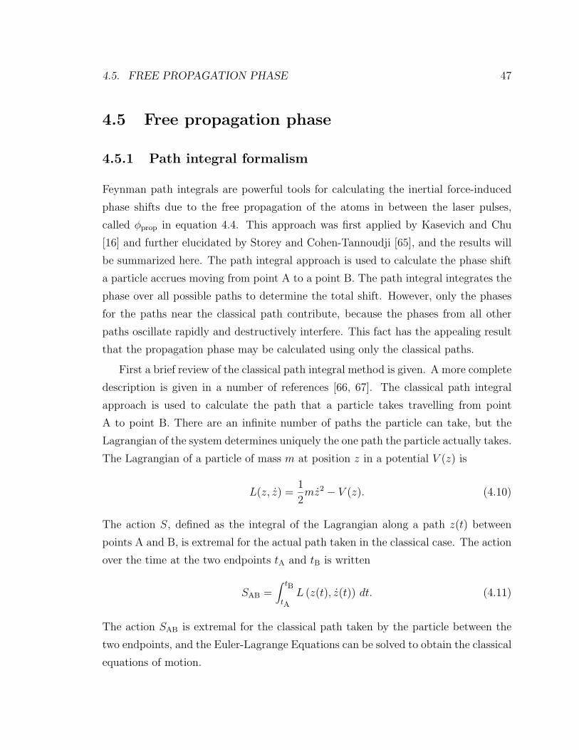
4.5. FREE PROPAGATION PHASE 47
4.5 Free propagation phase
4.5.1 Path integral formalism
Feynman path integrals are powerful tools for calculating the inertial force-induced
phase shifts due to the free propagation of the atoms in between the laser pulses,
called φprop in equation 4.4. This approach was first applied by Kasevich and Chu
[16] and further elucidated by Storey and Cohen-Tannoudji [65], and the results will
be summarized here. The path integral approach is used to calculate the phase shift
a particle accrues moving from point A to a point B. The path integral integrates the
phase over all possible paths to determine the total shift. However, only the phases
for the paths near the classical path contribute, because the phases from all other
paths oscillate rapidly and destructively interfere. This fact has the appealing result
that the propagation phase may be calculated using only the classical paths.
First a brief review of the classical path integral method is given. A more complete
description is given in a number of references [66, 67]. The classical path integral
approach is used to calculate the path that a particle takes travelling from point
A to point B. There are an infinite number of paths the particle can take, but the
Lagrangian of the system determines uniquely the one path the particle actually takes.
The Lagrangian of a particle of mass m at position z in a potential V (z) is
L(z, z) =1
2mz2 − V (z). (4.10)
The action S, defined as the integral of the Lagrangian along a path z(t) between
points A and B, is extremal for the actual path taken in the classical case. The action
over the time at the two endpoints tA and tB is written
SAB =∫ tB
tA
L (z(t), z(t)) dt. (4.11)
The action SAB is extremal for the classical path taken by the particle between the
two endpoints, and the Euler-Lagrange Equations can be solved to obtain the classical
equations of motion.
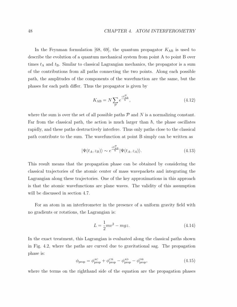
48 CHAPTER 4. ATOM INTERFEROMETRY
In the Feynman formulation [68, 69], the quantum propagator KAB is used to
describe the evolution of a quantum mechanical system from point A to point B over
times tA and tB. Similar to classical Lagrangian mechanics, the propagator is a sum
of the contributions from all paths connecting the two points. Along each possible
path, the amplitudes of the components of the wavefunction are the same, but the
phases for each path differ. Thus the propagator is given by
KAB = N∑P
eiSP
ABh , (4.12)
where the sum is over the set of all possible paths P and N is a normalizing constant.
Far from the classical path, the action is much larger than h, the phase oscillates
rapidly, and these paths destructively interfere. Thus only paths close to the classical
path contribute to the sum. The wavefunction at point B simply can be written as
|Ψ(tA, zB)〉 ∼ eiSP
ABh |Ψ(tA, zA)〉. (4.13)
This result means that the propagation phase can be obtained by considering the
classical trajectories of the atomic center of mass wavepackets and integrating the
Lagrangian along these trajectories. One of the key approximations in this approach
is that the atomic wavefunctions are plane waves. The validity of this assumption
will be discussed in section 4.7.
For an atom in an interferometer in the presence of a uniform gravity field with
no gradients or rotations, the Lagrangian is:
L =1
2mv2 −mgz. (4.14)
In the exact treatment, this Lagrangian is evaluated along the classical paths shown
in Fig. 4.2, where the paths are curved due to gravitational sag. The propagation
phase is:
φprop = φAC
prop + φCB
prop − φAD
prop − φDB
prop, (4.15)
where the terms on the righthand side of the equation are the propagation phases
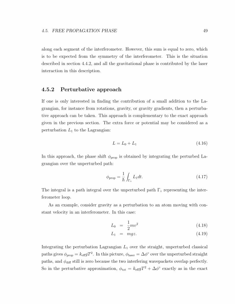
4.5. FREE PROPAGATION PHASE 49
along each segment of the interferometer. However, this sum is equal to zero, which
is to be expected from the symmetry of the interferometer. This is the situation
described in section 4.4.2, and all the gravitational phase is contributed by the laser
interaction in this description.
4.5.2 Perturbative approach
If one is only interested in finding the contribution of a small addition to the La-
grangian, for instance from rotations, gravity, or gravity gradients, then a perturba-
tive approach can be taken. This approach is complementary to the exact approach
given in the previous section. The extra force or potential may be considered as a
perturbation L1 to the Lagrangian:
L = L0 + L1 (4.16)
In this approach, the phase shift φprop is obtained by integrating the perturbed La-
grangian over the unperturbed path:
φprop =1
h
∫Γ
L1dt. (4.17)
The integral is a path integral over the unperturbed path Γ representing the inter-
ferometer loop.
As an example, consider gravity as a perturbation to an atom moving with con-
stant velocity in an interferometer. In this case:
L0 =1
2mv2 (4.18)
L1 = mgz. (4.19)
Integrating the perturbation Lagrangian L1 over the straight, unperturbed classical
paths gives φprop = keffgT2. In this picture, φlaser = ∆φ over the unperturbed straight
paths, and φdiff still is zero because the two interfering wavepackets overlap perfectly.
So in the perturbative approximation, φtot = keffgT2 + ∆φ exactly as in the exact
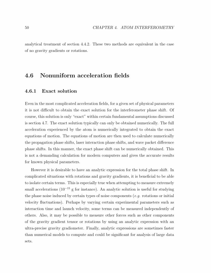
50 CHAPTER 4. ATOM INTERFEROMETRY
analytical treatment of section 4.4.2. These two methods are equivalent in the case
of no gravity gradients or rotations.
4.6 Nonuniform acceleration fields
4.6.1 Exact solution
Even in the most complicated acceleration fields, for a given set of physical parameters
it is not difficult to obtain the exact solution for the interferometer phase shift. Of
course, this solution is only “exact” within certain fundamental assumptions discussed
is section 4.7. The exact solution typically can only be obtained numerically. The full
acceleration experienced by the atom is numerically integrated to obtain the exact
equations of motion. The equations of motion are then used to calculate numerically
the propagation phase shifts, laser interaction phase shifts, and wave packet difference
phase shifts. In this manner, the exact phase shift can be numerically obtained. This
is not a demanding calculation for modern computers and gives the accurate results
for known physical parameters.
However it is desirable to have an analytic expression for the total phase shift. In
complicated situations with rotations and gravity gradients, it is beneficial to be able
to isolate certain terms. This is especially true when attempting to measure extremely
small accelerations (10−15 g for instance). An analytic solution is useful for studying
the phase noise induced by certain types of noise components (e.g. rotations or initial
velocity fluctuations). Perhaps by varying certain experimental parameters such as
interaction time and launch velocity, some terms can be measured independently of
others. Also, it may be possible to measure other forces such as other components
of the gravity gradient tensor or rotations by using an analytic expression with an
ultra-precise gravity gradiometer. Finally, analytic expressions are sometimes faster
than numerical models to compute and could be significant for analysis of large data
sets.
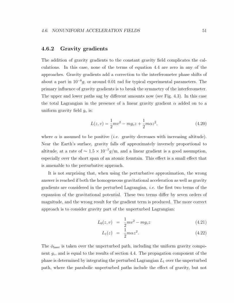
4.6. NONUNIFORM ACCELERATION FIELDS 51
4.6.2 Gravity gradients
The addition of gravity gradients to the constant gravity field complicates the cal-
culations. In this case, none of the terms of equation 4.4 are zero in any of the
approaches. Gravity gradients add a correction to the interferometer phase shifts of
about a part in 10−8g, or around 0.01 rad for typical experimental parameters. The
primary influence of gravity gradients is to break the symmetry of the interferometer.
The upper and lower paths sag by different amounts now (see Fig. 4.3). In this case
the total Lagrangian in the presence of a linear gravity gradient α added on to a
uniform gravity field g is:
L(z, v) =1
2mv2 −mgz +
1
2mαz2, (4.20)
where α is assumed to be positive (i.e. gravity decreases with increasing altitude).
Near the Earth’s surface, gravity falls off approximately inversely proportional to
altitude, at a rate of ∼ 1.5 × 10⁻⁷g/m, and a linear gradient is a good assumption,
especially over the short span of an atomic fountain. This effect is a small effect that
is amenable to the perturbative approach.
It is not surprising that, when using the perturbative approximation, the wrong
answer is reached if both the homogeneous gravitational acceleration as well as gravity
gradients are considered in the perturbed Lagrangian, i.e. the first two terms of the
expansion of the gravitational potential. These two terms differ by seven orders of
magnitude, and the wrong result for the gradient term is produced. The more correct
approach is to consider gravity part of the unperturbed Lagrangian:
L0(z, v) =1
2mv2 −mgz (4.21)
L1(z) =1
2mαz2. (4.22)
The φlaser is taken over the unperturbed path, including the uniform gravity compo-
nent g, and is equal to the results of section 4.4. The propagation component of the
phase is determined by integrating the perturbed Lagrangian L1 over the unperturbed
path, where the parabolic unperturbed paths include the effect of gravity, but not
52 CHAPTER 4. ATOM INTERFEROMETRY
that of the gravity gradient. Performing this integral gives:
φprop = αkeffT2
(7
12gT 2 − vT − z
). (4.23)
In this situation, the two interfering wavepackets do not overlap perfectly at the time
of the final π/2 pulse, as seen in Fig. 4.3. This wavepacket separation gives an extra
phase shift, and the total phase shift, to first order in α becomes:
φtot = keffgT 2 + αkeffT2
(7
12gT 2 − vT − z − h2
2mT
). (4.24)
In this equation, the acceleration experienced by the two wavepackets was integrated
over the two paths in order to determine their final separation and obtain φdiff. This
case of gravity plus a linear gravity gradient can be solved analytically. Taylor expand-
ing the analytic solution to first order in α yields the same expression as equation 4.24.
The perturbative approach works well for this case, giving good agreement with the
analytic solution; it is only in the presence of rotations as well that the perturbative
result begins to have difficulties.
4.6.3 Rotations
The presence of rotations vastly complicates the phase shift calculations. Rota-
tions deflect the trajectory of the wavepackets from the vertical and convert a one-
dimensional problem into a two- or three-dimensional problem. If the interferometer
encloses any physical area, as opposed to only enclosing area in the recoil diagram-
space, then a Sagnac phase shift due to the Coriolis acceleration will be included in
the interferometer phase shift [70]. Additionally, centrifugal forces contribute phase
shifts to the atoms in the presence of rotations. These phase shift are calculated
similarly to the above gravitational phase shift, and the resulting phase shift for a
rotation Ω is:
φrot = 2keff·(v ×Ω)T 2 + keff·(Ω×(Ω× r))T 2. (4.25)
4.7. LIMITATIONS TO THE THEORY 53
The first term is the Coriolis term, while the second is due to centrifugal acceleration.
Typically a perturbative approximation is used to calculate the influence of rotations
on the interferometer phase for a gravimeter or gradiometer, as the rotation phase
shifts are generally small in these configurations. The relative magnitudes of the
two rotation terms depends on the exact interferometer geometry, particularly the
alignment of the atomic fountain.
In the pursuit of the high precision measurements needed to test General Relativity
and seek new forces as described in section 2.3, the accuracy of the analytic results
of the perturbative method was examined. Several attempts have been made to
examine the higher order corrections [22, 71], but they fall short at around 10−10g.
Several colleagues performed a series of calculations designed to test the perturbative
result to higher orders using a Taylor expansion approach [72]. The approach was as
follows: in the rotating frame, i.e. the lab frame, the equations of motion were solved
analytically using only uniform gravity and rotations. The perturbative path integral
approach was then used to calculate the free propagation phase shift by integrating
the Lagrangian, including gravity gradients, over the equations of motion. This path
integral was carried out by Taylor expanding the Lagrangian and integrating over the
Taylor expanded equations of motion. This approach results in an analytic solution,
albeit a complicated one, that agrees with the exact numerical calculations to a part
per 1016 when the expansion is carried out to seventh order. This level is better than
even the anticipated performance for a space-based gradiometer (see section 8.2). In
this approach, higher order curvature is neglected, which contributes at about the
level of the last digit (which is where the second order gradient correction enters).
4.7 Limitations to the theory
The numerical solutions labelled as “exact” here are only accurate within the frame-
work of the approximations made in the theory. There are several fundamental as-
sumptions to the theory presented here, particularly to the path integral approach of
finding the free propagation phase, which bear a closer look. These approximations
are certainly sufficient for almost all practical gradient sensing applications, which
54 CHAPTER 4. ATOM INTERFEROMETRY
usually require precision no better than 10−10g. However for the ultra-precise tests
of General Relativity and searches for new physics discussed in section 2.3, some of
the approximations may not be sufficient.
One of the fundamental approximations to the path integral method is to approx-
imate the Gaussian atomic wavepackets as plane waves. To some degree it seems like
a very poor approximation to do this, and it is surprising that the method works as
well as it does. The reason for the success of the approximation is that the atomic
wavepackets are essentially plane waves within a Gaussian envelope. In fact, the
atomic wavepackets produced by the MOT are near Heisenberg-limited wavepackets.
Initially the MOT localizes the atom to < λ/2 and a temperature around 1µK, which
produces a wavepacket near the Heisenberg limit6. To determine fully the phase shifts
for Gaussian wavepackets, the approach is to integrate numerically the entire wave-
packet using the path integral method. Spreading of the Gaussian wavepacket must
be considered, as well as distortion to the presence of gravity gradients. This is a
difficult proposition and is only potentially a concern for precisions of the order of
< 10−15g.
In some gravitational fields the Lagrangian is not quadratic. Again, in this case,
the path integral approach will break down. This is not due to a limitation in the
theory of Storey and Cohen-Tannoudji, but rather in that of Feynman’s original
path integral theory. Feynman only proved the path integral approach to quantum
mechanics for quadratic Lagrangians [68]. It is conceivable that for complicated
gravitational potentials, the limit of only integrating along the classical path is not
valid. The problem might become a true “quantum problem” requiring integration
over a large number of non-classical paths. In this case, a direct numerical integration
of the Schrodinger equation is called for. It is unlikely any analytic solution exists for
this regime. Such a breakdown in the theory is only conceivable in the near-field limit
of large test masses close to the proof masses. In the far field limit, the gravitational
contribution to the Lagrangian is always quadratic (assuming a reference frame that
is at most slowly rotating).
6The full description of atoms in a MOT is a complicated proposition requiring solving the Fokker-Planck equation, but the approximation of Heisenberg-limited Gaussian wavepackets is a reasonableone.
4.8. APPLICATION TO GRADIOMETRY 55
Another approximation in the theory lies in the laser-atom interactions. In sec-
tion 3.7 the theory of stimulated Raman transitions was described using the short,
intense pulse limit. The length of the Raman pulses was neglected since it is typ-
ically four orders of magnitude shorter than the interferometer interrogation time.
For ultra-precise measurements, it is certainly called for to integrate the phase over
the envelope of the Raman pulses. Even more than this effect, the fundamental pro-
cess of the Raman transition needs to be studied. Questions regarding what happens
during the Raman transition need elucidating. During the transition itself, the atom
certainly behaves non-classically, and there is not a single point where momentum is
instantaneously imparted to the wavepackets. Such questions merit full integration
of the Schrodinger Equation.
4.8 Application to gradiometry
So far, the theory has been described only for single interferometer gravimeters. By
taking two spatially-separated interferometers and directly subtracting the interfer-
ometer phases, a phase proportional to the gravity gradient is obtained7. Explicitly,
the gradiometer phase shift is the difference of the total interferometer phase shifts
for the two gravimeters:
∆φ = φ(1)tot − φ
(2)tot, (4.26)
where 1 and 2 represent the two gravimeters. In the case of a linear gravity gradient
on top of a uniform gravity field with no rotations, this phase reduces to:
∆φ = keffT2α
(z(1) − z(2)
)+
(∆φ
(1) − ∆φ(2)
), (4.27)
where z(1) and z(2) are the initial positions of the two atom ensembles. This solution
is obtained considering the gravity gradient in each interferometer in the perturba-
tive limit. Note that φdiff drops out as it depends only on the gravity gradient at
each interferometer, and that gradient is assumed to be linear and constant here.
Additionally, the large first order gravity shift cancels as expected. The first term of
7This phase is modulo 2π but is typically less than 2π for most of the gravity gradients involved.
56 CHAPTER 4. ATOM INTERFEROMETRY
equation 4.27 is just the difference in gravity between the initial positions of the two
accelerometers and is usually written as keffδgT2.
The key virtue of gradiometers is manifested in the second term of equation 4.27.
As described in section 4.4.2, this term contains the acceleration noise induced by
vibrations of the reference platform (the optical table containing the Raman lasers)
which plagues gravimeters. However, because the same reference platform is used and
the same lasers simultaneously drive the two interferometers ∆φ(1)−∆φ
(2) = 0. In the
instance of perfect common-mode coupling of the two gravimeters, the gradiometer
is completely immune to reference platform noise. It is this immunity to vibrational
noise that makes gravity gradiometers the instruments of choice for mobile studies of
gravity and studies requiring extremely high precision.
Another important benefit of gradiometers is that several of the higher order
effects discussed in the previous section have a high degree of commonality between
the two gravimeters8, which lessens the constraints on the rigor of the calculations.
For instance, the second order curvature of the Earth’s field is only ∼ 10−6 Tzz over
1 m, and can be safely neglected if the measurement baseline is not too large and the
required instrument accuracy is less than this level. Other effects, such as changing
gravity due to tides, i.e. changing gravitational attraction due to the position of the
Sun and the moon, contribute to a gravimeter at 10−7g, but to a 10 m gradiometer
at 10−12g, and again this effect can be neglected for most applications.
Of final note is that the accuracy of the gravity gradiometer is limited by the
accuracy to which the separation between the two accelerometers is known. The
uncertainty of the spacing leads to an uncertainty in the gradient in a linear fashion.
However for the purposes of the measurements contained herein, video imaging of
the position of the atom ensembles is sufficient to locate them within the chambers
to around 0.1 mm, and the spacing between the chambers is measured to similar
accuracy. This is an uncertainty of approximately one part in 104, which is sufficient
for this dissertation.
8This is particularly true for far-field mass distributions and not necessarily the case for complexgravity fields typical of near-field masses.
Chapter 5
Experimental Apparatus
5.1 Apparatus overview
The apparatus consists of two laser cooled and trapped sources of Cs atoms in two
separate ultra-high vacuum (UHV) chambers. The atoms are launched on ballistic
trajectories and prepared in a particular internal state with optical and microwave
techniques before undergoing the interferometer sequence. Following the interferom-
eter sequence, atoms are detected using a normalizing detection method. The total
cycle time is 0.7 - 1.4 s, depending on the trap loading parameters. Each of these
stages is described below. In addition, the operation of an actively controlled vibra-
tion isolation system which is used to validate the data acquisition methodology is
described. Finally, the subsystem for generating microwaves is described. A picture
of the gravity gradiometer apparatus is shown in Fig. 5.1.
5.2 Vacuum system
5.2.1 Motivation for vacuum
Laser cooling and trapping experiments need to be performed in a region of UHV.
There are two main considerations that determine what level of vacuum is necessary:
loading of the MOT and coherence in the interferometer. The MOT is loaded from
57
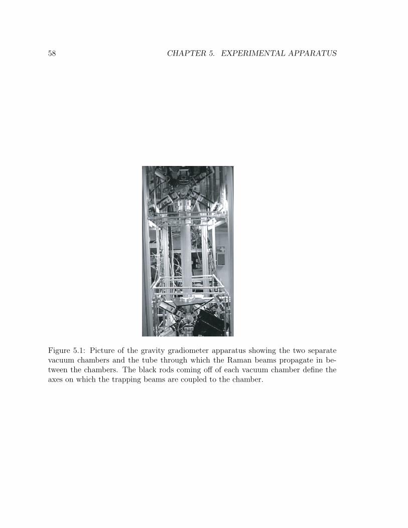
58 CHAPTER 5. EXPERIMENTAL APPARATUS
Figure 5.1: Picture of the gravity gradiometer apparatus showing the two separatevacuum chambers and the tube through which the Raman beams propagate in be-tween the chambers. The black rods coming off of each vacuum chamber define theaxes on which the trapping beams are coupled to the chamber.
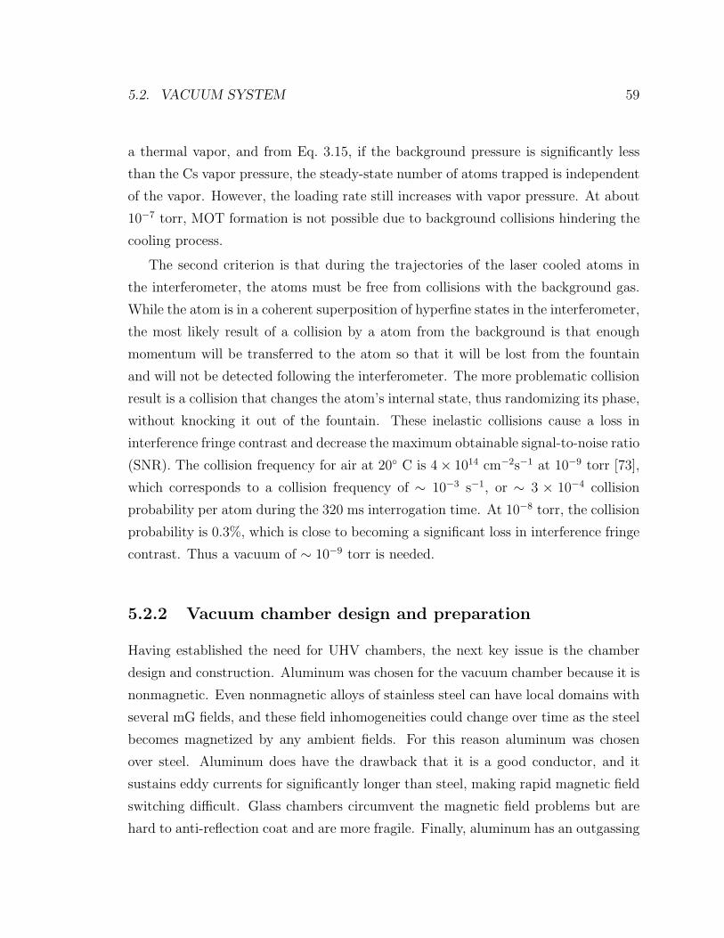
5.2. VACUUM SYSTEM 59
a thermal vapor, and from Eq. 3.15, if the background pressure is significantly less
than the Cs vapor pressure, the steady-state number of atoms trapped is independent
of the vapor. However, the loading rate still increases with vapor pressure. At about
10−7 torr, MOT formation is not possible due to background collisions hindering the
cooling process.
The second criterion is that during the trajectories of the laser cooled atoms in
the interferometer, the atoms must be free from collisions with the background gas.
While the atom is in a coherent superposition of hyperfine states in the interferometer,
the most likely result of a collision by a atom from the background is that enough
momentum will be transferred to the atom so that it will be lost from the fountain
and will not be detected following the interferometer. The more problematic collision
result is a collision that changes the atom’s internal state, thus randomizing its phase,
without knocking it out of the fountain. These inelastic collisions cause a loss in
interference fringe contrast and decrease the maximum obtainable signal-to-noise ratio
(SNR). The collision frequency for air at 20 C is 4× 1014 cm−2s−1 at 10−9 torr [73],
which corresponds to a collision frequency of ∼ 10−3 s−1, or ∼ 3 × 10⁻⁴ collision
probability per atom during the 320 ms interrogation time. At 10−8 torr, the collision
probability is 0.3%, which is close to becoming a significant loss in interference fringe
contrast. Thus a vacuum of ∼ 10−9 torr is needed.
5.2.2 Vacuum chamber design and preparation
Having established the need for UHV chambers, the next key issue is the chamber
design and construction. Aluminum was chosen for the vacuum chamber because it is
nonmagnetic. Even nonmagnetic alloys of stainless steel can have local domains with
several mG fields, and these field inhomogeneities could change over time as the steel
becomes magnetized by any ambient fields. For this reason aluminum was chosen
over steel. Aluminum does have the drawback that it is a good conductor, and it
sustains eddy currents for significantly longer than steel, making rapid magnetic field
switching difficult. Glass chambers circumvent the magnetic field problems but are
hard to anti-reflection coat and are more fragile. Finally, aluminum has an outgassing
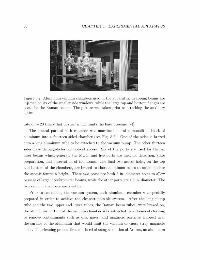
60 CHAPTER 5. EXPERIMENTAL APPARATUS
Figure 5.2: Aluminum vacuum chambers used in the apparatus. Trapping beams areinjected on six of the smaller side windows, while the large top and bottom flanges areports for the Raman beams. The picture was taken prior to attaching the auxiliaryoptics.
rate of ∼ 20 times that of steel which limits the base pressure [74].
The central part of each chamber was machined out of a monolithic block of
aluminum into a fourteen-sided chamber (see Fig. 5.2). One of the sides is brazed
onto a long aluminum tube to be attached to the vacuum pump. The other thirteen
sides have through-holes for optical access. Six of the ports are used for the six
laser beams which generate the MOT, and five ports are used for detection, state
preparation, and observation of the atoms. The final two access holes, on the top
and bottom of the chambers, are brazed to short aluminum tubes to accommodate
the atomic fountain height. These two ports are both 3 in. diameter holes to allow
passage of large interferometer beams, while the other ports are 1.5 in. diameter. The
two vacuum chambers are identical.
Prior to assembling the vacuum system, each aluminum chamber was specially
prepared in order to achieve the cleanest possible system. After the long pump
tube and the two upper and lower tubes, the Raman beam tubes, were brazed on,
the aluminum portion of the vacuum chamber was subjected to a chemical cleaning
to remove contaminants such as oils, gases, and magnetic particles trapped near
the surface of the aluminum that would limit the vacuum or cause stray magnetic
fields. The cleaning process first consisted of using a solution of Ardrox, an aluminum
5.2. VACUUM SYSTEM 61
penetrant, for 15 min. at 140 F to remove certain magnetic materials. Next, after a
high-pressure rinsing with water, the chamber was soaked in an aluminum pickle for
∼ 30 s to further clean the chamber. Following another rinsing, a 3 min. soak in 30%
nitric acid removed any remaining surface contaminants. Finally, the chambers were
rinsed with several successively more pure baths of high-pressure heated de-ionized
water. These steps were necessary to achieve the lowest possible base pressure and
obtain the least magnetic chamber possible using aluminum. Finally a coating of
Vac-Seal, a commercial UHV sealant, was applied to the outside of each brazed joint
in order to seal a few small micro-leaks.
Following the rigorous chamber cleaning, the sealing of the vacuum chamber is
accomplished as follows. An anti-reflection coated glass window seals each port by
means of an indium seal1. Each indium seal consists of a length of 1 mm diameter
indium wire formed into a ring slightly smaller than the diameter of the window. The
vacuum seal is formed simply by tightening the window down using an aluminum
retaining ring placed on top of the window. A mylar spacer ring is placed between the
retaining ring and the window to evenly distribute the force applied by the retaining
ring in order to keep the window from shattering. The aluminum bolts used to tighten
the retaining ring need only be tightened about one quarter turn past finger tight to
flatten the indium and make a tight seal. Indium seals can always be tightened further
when the vacuum chamber is tested for leaks.
Prior to evacuating the chamber, the Cs reservoir is prepared and attached to the
chamber. A glass ampoule containing 5 g of Cs is placed inside a narrow vacuum tube
whose inner diameter is barely large enough to accommodate the ampoule. This tube
is attached to a glass tube to be used as the temperature controlled reservoir, called
the cold finger. This assembly is evacuated with a turbo-molecular pump, baked for
several days at ∼ 200 C to remove gases trapped on the walls of the assembly, and
then sealed off from the pump. The Cs ampoule is broken by squeezing the narrow
tube containing it with a C-clamp until the glass shatters. The tip of the cold finger
is cooled to ∼ −30 C and the rest of the chamber is kept heated in order to collect
1For these windows, the surface quality of each window is only λ/4, as the wavefront distortionof the trapping beams is not as critical as the Raman lasers.
62 CHAPTER 5. EXPERIMENTAL APPARATUS
the Cs in the cold finger. After maintaining these temperatures for several days, all
the Cs accumulates in the cold finger, and the cold finger is valved-off and attached
to the aluminum vacuum chamber on one of the five side ports not used for the MOT
laser beams.
5.2.3 Chamber evacuation
The chamber is sealed and evacuated with a 25 l/s noble diode ion pump (Varian
9115050) attached to the end of the long aluminum pump tube. The pump tube is
long to place the magnet for the ion pump as far as possible from the interferometer
region of the chamber. The chamber is first evacuated with a turbo-molecular pump
backed by an oil-free diaphragm pump. Then the chamber is heated for one week to
degas the chamber walls. The aluminum parts of the chamber are baked at ∼ 100 C
(60 below the melting point of indium), and the steel portions of the chamber are
heated to 250 C. Following the bake-out, the ion pump is turned on, the chamber is
valved-off from the external pumps, and the base pressure falls below 5× 10⁻¹⁰ torr,
using the ion pump current as a pressure gauge. The pressure slowly rises to an
equilibrium pressure of ∼ 9× 10⁻¹⁰ torr due to outgassing of the aluminum chamber.
This base pressure is sufficient to not limit the MOT loading or the interferometer
fringe contrast.
Finally, the temperature of the Cs cold finger is brought to 10 C, and the valve
to the main chamber is opened. It takes about a day for the Cs partial pressure to
build up enough to load a MOT with sufficiently large numbers, because the Cs vapor
adsorbs onto the clean chamber walls until a monolayer has built up. The Cs partial
pressure is adjusted by either control of the cold finger temperature or by adjusting
the valve between the cold finger and the central chamber.
It should be noted that the positioning of the cold finger is critical. If the cold
finger is too far away from the central chamber, i.e. at the end of the long pump tube
near the vacuum pump, it takes a long time (greater than a week) for the pressure in
the trapping region to become large enough to form a MOT. This long time is because
the entire length of the pump tube must be coated with a monolayer of Cs, and the
5.3. LASER SYSTEM 63
bulk of the Cs gets pumped by the ion pump first. Ion pumps are not designed
to pump large concentrations of metal vapors like Cs. Therefore, placing the cold
finger near the pump will ultimately cause filaments of Cs to form between the anode
and cathode of the ion pump, causing a leakage current to flow, giving an erroneous
pressure reading and limiting the pump lifetime and speed. Baking the pump again
or applying a high voltage of ∼ 20 kV to the pump will remove these filaments, but
this process cannot be extended indefinitely without shortening the life of the pump.
Therefore, the cold finger is placed directly on the vacuum chamber as close to the
trapping region and as far away from the ion pump as possible. Additionally, the
inside of the pump tube is coated with graphite, which increases the adsorption of Cs
because of its large surface area, thereby increasing the lifetime of the pump.
5.3 Laser system
The laser system for cooling, trapping, state preparation, and atom detection consists
of a frequency stabilized master laser and several power amplifiers. Several configura-
tions based on different types of lasers were used. This section discusses the relative
merits of the various laser configurations used and also describes the frequency control
and light delivery elements common to all of the laser systems employed2.
5.3.1 Master laser
In order to obtain a source of cold atoms with minimal fluctuations, the master laser
must be frequency stabilized and have a narrow intrinsic linewidth. In the proof-
of-principle gradiometer experiment, a distributed Bragg reflector (DBR) laser (SDL
5712) was the master laser. In subsequent experiments an external cavity, grating-
stabilized laser (New Focus Vortex) replaced the DBR. The master laser frequency
must be near the F = 4 → F′ = 5, so the master laser is locked several hundred
MHz below this frequency in order to accommodate the frequency shifts necessary
for dynamic frequency control.
2For a detailed description of many of the standard optical elements used in atomic physicsexperiments see [75, 76] for instance.
64 CHAPTER 5. EXPERIMENTAL APPARATUS
The master laser is frequency stabilized to an atomic resonance in Cs vapor us-
ing a modulation transfer saturated spectroscopy lock [77]. The lock setup is the
same as was used in [70]. A small amount of light (∼ 1 mW) is picked off from
the master laser and sent to the locking optics. This beam further is split into two
beams: the pump and the probe beams for the saturation lock. The pump beam is
double-passed through an 80 MHz acousto-optic modulator (AOM, Isomet 1205C).
A Hewlett Packard 8770 arbitrary waveform generator (AWG) generates a radio fre-
quency (rf) frequency modulated (FM) waveform that drives the AOM. The pump
beam then propagates through a 3 in. glass cell containing Cs vapor. The probe
beam counterpropagates through the Cs cell collinear with the pump beam, and the
FM on the pump beam is translated into amplitude modulation (AM) on the probe
beam near the narrow atomic resonances. The AM probe is detected on a photodiode
(Thorlabs FDS-100) and demodulated using a lock-in amplifier (Stanford Research
Systems SRS810). The frequency is actively stabilized to one of the resonances, using
proportional, integral, and differential (PID) feedback to the laser controller.
Originally, a DBR laser was the master laser. This laser was locked to the 4/5
crossover resonance of the F = 4 → F′ = 5 transition using an AOM frequency of
72 MHz, with a modulation frequency of 50 kHz and a modulation depth of ∼ 8 MHz.
The intrinsic linewidth of the DBR was 3 MHz. The DBR was also particularly
sensitive to optical feedback. All lasers in the experiment use double-stage optical
isolators (Optics for Research IOT-2.7-852-LP) which provide 60 dB of isolation from
back reflections. However the small amount of light that is backscattered from the
anti-reflection coated front window of the isolator is enough feedback to create a cavity
and perturb the DBR frequency. For this reason the isolator is slightly misaligned,
and an aluminum tie-rod is attached to the isolator and the laser mount in order to
stabilize the length of the cavity formed by backscattering and to minimize changes
in the frequency shifts from feedback.
In work subsequent to the proof-of-principle work, a Vortex grating stabilized laser
replaced the DBR as the master laser. Because of its extended cavity, the Vortex has
a linewidth of 300 kHz, ten times narrower than that of the DBR. The Vortex laser
is located in the neighboring lab and is locked to the same Cs resonance as the DBR
5.3. LASER SYSTEM 65
was. The locked laser has a stability of 1 kHz/√
Hz. Light from the Vortex laser
is coupled into a 20 m polarization maintaining (PM) optical fiber and delivered to
the gradiometer lab. This light then injection locks the DBR laser at an identical
frequency as when the DBR was independently locked [78]. The injection-locked DBR
takes on the spectral properties of the Vortex laser which seeds it, thereby reducing
its linewidth significantly [79]. The more stable master laser reduces the shot-to-shot
rms number fluctuations of the MOTs by a factor of five to a SNR of 200:1. In
addition, frequency induced noise during the detection of the atoms following the
interferometer is greatly reduced.
5.3.2 Laser amplifiers
The MOTs require higher laser powers than the master provides, necessitating the
use of amplifier lasers to generate sufficient power for cooling and trapping. The
amplifier lasers are all injection locked with the master laser in a master oscillator-
power amplifier configuration. The injection locks transfer the frequency stability of
the master laser, without addition of extra frequency or intensity noise [79]. Before
injecting the slave lasers, the master laser is split in two, and each half if sent through
a double-passed AOM. These AOMs are the principal frequency-control AOMs for
the trapping and detection beams, and they allow differential frequency control for
the two amplifier lasers, one for the upward-pointing set of trapping beams and one
for the downward-pointing set of trapping beams. Additionally, two different types of
amplifiers were used, tapered amplifiers and standard single-mode amplifier diodes,
and their relative merits are discussed here.
Tapered amplifiers
Tapered amplifiers are 500 mW laser diodes (SDL 8630E). By using a tapered gain
region, the gain does not saturate as in standard rectangular gain regions, and higher
output powers are achievable [80]. Because of the taper, the amplifier output is highly
elliptical, ∼ 100 : 1 aspect ratio. A 2.8 mm aspheric lens is used to collimate the
output in one dimension, and a 35 mm cylindrical lens is used to collimate the other
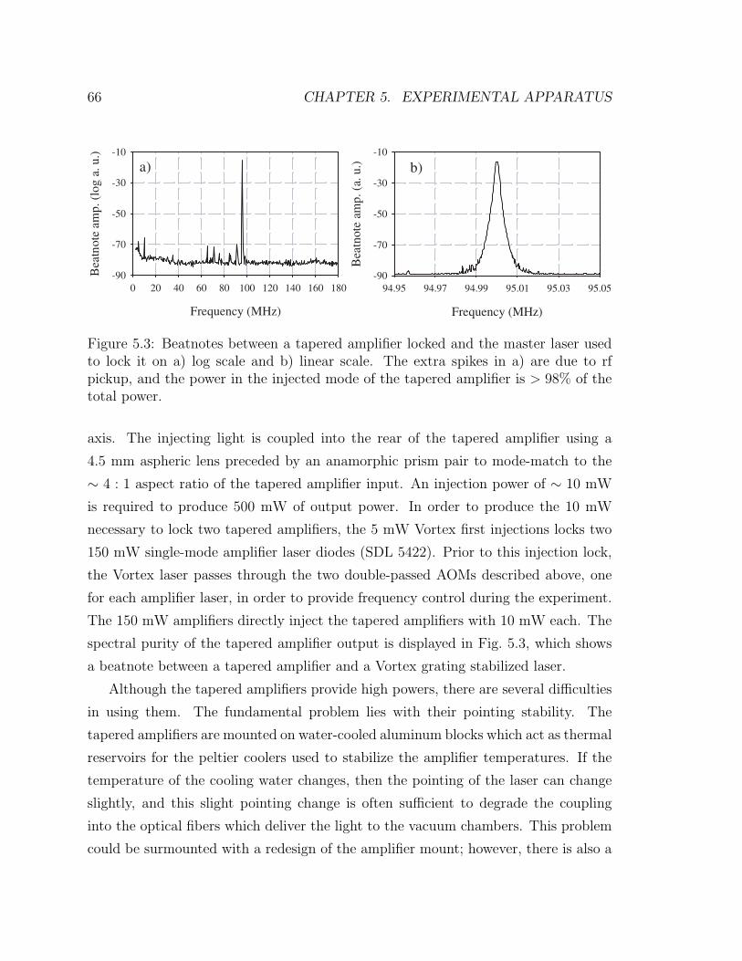
66 CHAPTER 5. EXPERIMENTAL APPARATUS
Frequency (MHz)
0 20 40 60 80 100 120 140 160 180
Bea
tnot
e am
p. (
log
a. u
.)
-90
-70
-50
-30
-10
Frequency (MHz)
94.95 94.97 94.99 95.01 95.03 95.05
Bea
tnot
e am
p. (
a. u
.)
-90
-70
-50
-30
-10
a) b)
Figure 5.3: Beatnotes between a tapered amplifier locked and the master laser usedto lock it on a) log scale and b) linear scale. The extra spikes in a) are due to rfpickup, and the power in the injected mode of the tapered amplifier is > 98% of thetotal power.
axis. The injecting light is coupled into the rear of the tapered amplifier using a
4.5 mm aspheric lens preceded by an anamorphic prism pair to mode-match to the
∼ 4 : 1 aspect ratio of the tapered amplifier input. An injection power of ∼ 10 mW
is required to produce 500 mW of output power. In order to produce the 10 mW
necessary to lock two tapered amplifiers, the 5 mW Vortex first injections locks two
150 mW single-mode amplifier laser diodes (SDL 5422). Prior to this injection lock,
the Vortex laser passes through the two double-passed AOMs described above, one
for each amplifier laser, in order to provide frequency control during the experiment.
The 150 mW amplifiers directly inject the tapered amplifiers with 10 mW each. The
spectral purity of the tapered amplifier output is displayed in Fig. 5.3, which shows
a beatnote between a tapered amplifier and a Vortex grating stabilized laser.
Although the tapered amplifiers provide high powers, there are several difficulties
in using them. The fundamental problem lies with their pointing stability. The
tapered amplifiers are mounted on water-cooled aluminum blocks which act as thermal
reservoirs for the peltier coolers used to stabilize the amplifier temperatures. If the
temperature of the cooling water changes, then the pointing of the laser can change
slightly, and this slight pointing change is often sufficient to degrade the coupling
into the optical fibers which deliver the light to the vacuum chambers. This problem
could be surmounted with a redesign of the amplifier mount; however, there is also a
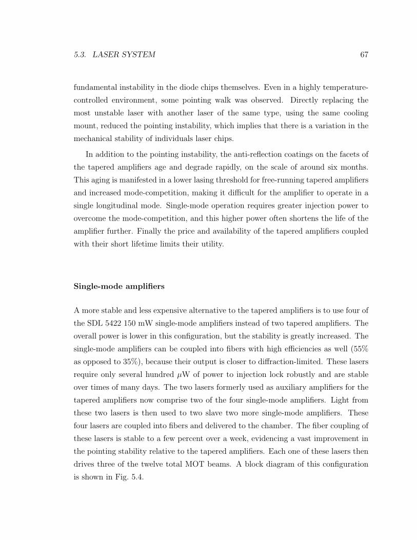
5.3. LASER SYSTEM 67
fundamental instability in the diode chips themselves. Even in a highly temperature-
controlled environment, some pointing walk was observed. Directly replacing the
most unstable laser with another laser of the same type, using the same cooling
mount, reduced the pointing instability, which implies that there is a variation in the
mechanical stability of individuals laser chips.
In addition to the pointing instability, the anti-reflection coatings on the facets of
the tapered amplifiers age and degrade rapidly, on the scale of around six months.
This aging is manifested in a lower lasing threshold for free-running tapered amplifiers
and increased mode-competition, making it difficult for the amplifier to operate in a
single longitudinal mode. Single-mode operation requires greater injection power to
overcome the mode-competition, and this higher power often shortens the life of the
amplifier further. Finally the price and availability of the tapered amplifiers coupled
with their short lifetime limits their utility.
Single-mode amplifiers
A more stable and less expensive alternative to the tapered amplifiers is to use four of
the SDL 5422 150 mW single-mode amplifiers instead of two tapered amplifiers. The
overall power is lower in this configuration, but the stability is greatly increased. The
single-mode amplifiers can be coupled into fibers with high efficiencies as well (55%
as opposed to 35%), because their output is closer to diffraction-limited. These lasers
require only several hundred µW of power to injection lock robustly and are stable
over times of many days. The two lasers formerly used as auxiliary amplifiers for the
tapered amplifiers now comprise two of the four single-mode amplifiers. Light from
these two lasers is then used to two slave two more single-mode amplifiers. These
four lasers are coupled into fibers and delivered to the chamber. The fiber coupling of
these lasers is stable to a few percent over a week, evidencing a vast improvement in
the pointing stability relative to the tapered amplifiers. Each one of these lasers then
drives three of the twelve total MOT beams. A block diagram of this configuration
is shown in Fig. 5.4.
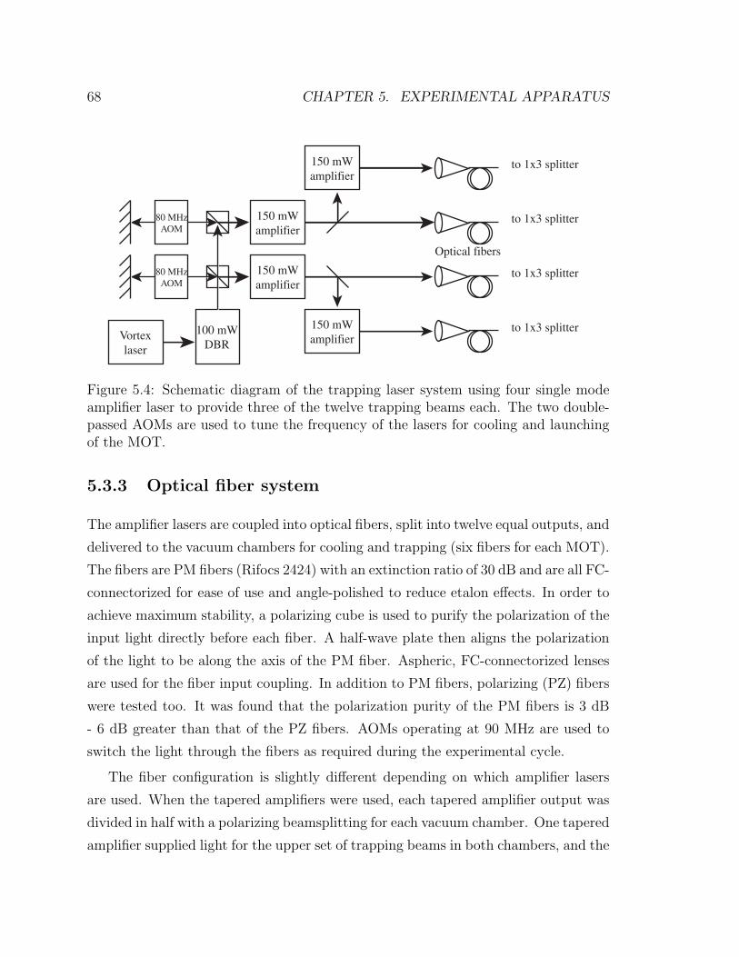
68 CHAPTER 5. EXPERIMENTAL APPARATUS
150 mWamplifier
80 MHzAOM
Optical fibers
100 mWDBR
Vortexlaser
80 MHzAOM
150 mWamplifier
150 mWamplifier
150 mWamplifier
to 1x3 splitter
to 1x3 splitter
to 1x3 splitter
to 1x3 splitter
Figure 5.4: Schematic diagram of the trapping laser system using four single modeamplifier laser to provide three of the twelve trapping beams each. The two double-passed AOMs are used to tune the frequency of the lasers for cooling and launchingof the MOT.
5.3.3 Optical fiber system
The amplifier lasers are coupled into optical fibers, split into twelve equal outputs, and
delivered to the vacuum chambers for cooling and trapping (six fibers for each MOT).
The fibers are PM fibers (Rifocs 2424) with an extinction ratio of 30 dB and are all FC-
connectorized for ease of use and angle-polished to reduce etalon effects. In order to
achieve maximum stability, a polarizing cube is used to purify the polarization of the
input light directly before each fiber. A half-wave plate then aligns the polarization
of the light to be along the axis of the PM fiber. Aspheric, FC-connectorized lenses
are used for the fiber input coupling. In addition to PM fibers, polarizing (PZ) fibers
were tested too. It was found that the polarization purity of the PM fibers is 3 dB
- 6 dB greater than that of the PZ fibers. AOMs operating at 90 MHz are used to
switch the light through the fibers as required during the experimental cycle.
The fiber configuration is slightly different depending on which amplifier lasers
are used. When the tapered amplifiers were used, each tapered amplifier output was
divided in half with a polarizing beamsplitting for each vacuum chamber. One tapered
amplifier supplied light for the upper set of trapping beams in both chambers, and the
5.4. LASER COOLED ATOMIC SOURCES 69
other supplied light for the lower set of trapping beams. In this way, identical light
was used for the MOTs in each chamber, which provided a high degree of common-
mode behavior between the two MOTs. After being split in two, each amplifier laser
was further split into three equal outputs using a fiber beamsplitter system. The fiber
splitters (Optics for Research Fiberbench system) consist of a polarizer to purify the
polarization after the input fiber, half-wave plates and calcite polarizers to divide the
beam into three equal outputs, and half-wave plates to align the polarization to the
fiber. These fiber splitters are all low-profile optics mounted on a small steel base
and have excellent stability (a few percent drift over several months). When the four
separate 150 mW lasers are used to power the MOTs, each laser is coupled into a PM
fiber and then into a three-way splitter. Each laser powers either the top set of three
beams or the bottom set of three beams for one of the two MOTs.
5.4 Laser cooled atomic sources
The main purpose of the quiet, stable laser system is to to obtain a bright source
of cold atoms with minimal fluctuations in number. The trapping beams from the
twelve fibers are delivered to the two vacuum chambers and are allowed to propagate
uncollimated to the two MOTs. The beams first pass through a polarizing cube to
purify the polarization and a quarter-wave plate to give the appropriate helicity for
trapping. The MOTs are in the (1,1,1) configuration, i.e. with three beams pointing
downward and three beams pointing upward. The polarizations of the beams are
σ+ − σ− for opposing beams. By not collimating the beams, the beam size limit
imposed by the window apertures was circumvented. Using uncollimated beams for
the MOTs gives a factor of two improvement in total number of atoms trapped versus
collimated beams. The approximate beam waist at the trapping position is 2.5 cm
(1/e2), and the intensity is about 1.2 Isat per beam. The trapping beams are detuned
8 MHz to the red of the F = 4 → F′ = 5 cooling transition.
The MOTs are loaded from a thermal vapor of Cs. The Cs reservoir in the
cold finger is maintained at ∼ 10 C by a thermoelectric cooler. The exact Cs partial
pressure is maintained by operating with the cold finger valve partially open to control
70 CHAPTER 5. EXPERIMENTAL APPARATUS
the flow of Cs to the trapping region. The optimal vapor pressure is chosen by opening
the valve until the number of atoms detected after the fountain ceases to increase.
If opened further, the increased vapor pressure reduces the number of atoms in the
MOT due to collisions with untrapped atoms during the atomic fountain. At around
this vapor pressure, collisions start to decrease interferometer contrast as well. With
optimal vapor pressure and optimized loading parameters, the traps contain about
2 × 10⁸ atoms in each MOT.
After loading the MOTs from a thermal vapor for 1 s, the molasses beam detun-
ing is increased to 20 MHz in order to compress the MOTs. Then the cold atoms
are launched in ballistic trajectories in atomic fountains. The trapping quadrupole
magnetic fields are turned off prior to launching. Because the vacuum chambers are
aluminum, the atoms must be held in the 20 MHz detuned optical molasses for 30 ms
while the eddy currents from the field switching damp out3. Following this holding
period, for each MOT, the frequency of the upper three molasses beams are ramped
down by 1 MHz over 5 ms using the double-passed AOM for frequency control, while
the frequency of the lower three beams is ramped up by an equal amount. This fre-
quency ramp smoothly transfers the atoms to an optical molasses moving at 1.5 m/s
(see Fig. 5.5). This ramp is necessary to transfer all atoms to the moving frame,
as a discontinuous jump into the moving frame leaves a significant portion of the
atoms behind. To cool the atoms to a final temperature of 2.3 µK, the frequency
of the trapping beams is stepped down to about 40 MHz detuned, still in a moving
molasses, and the intensity is ramped down to half intensity in 1 ms, held for 0.5 ms,
and ramped completely off in 0.5 ms more. All of the frequency and intensity ramps
are accomplished using direct digital synthesis from the Hewlett Packard HP8770A
AWGs and are highly stable. Following this launching and cooling phase, the cold
atoms move freely in a 320 ms, 12 cm high fountain during which they are prepared
in a special state and then interrogated by the interferometer sequence.
3In retrospect, a chamber constructed out of titanium alloy or glass would have solved thisproblem without sacrificing the magnetic purity of aluminum. However, precision machined titaniumis expensive and glass is difficult to anti-reflection coat in the required chamber geometry. Futuredesigns most likely will employ different materials.
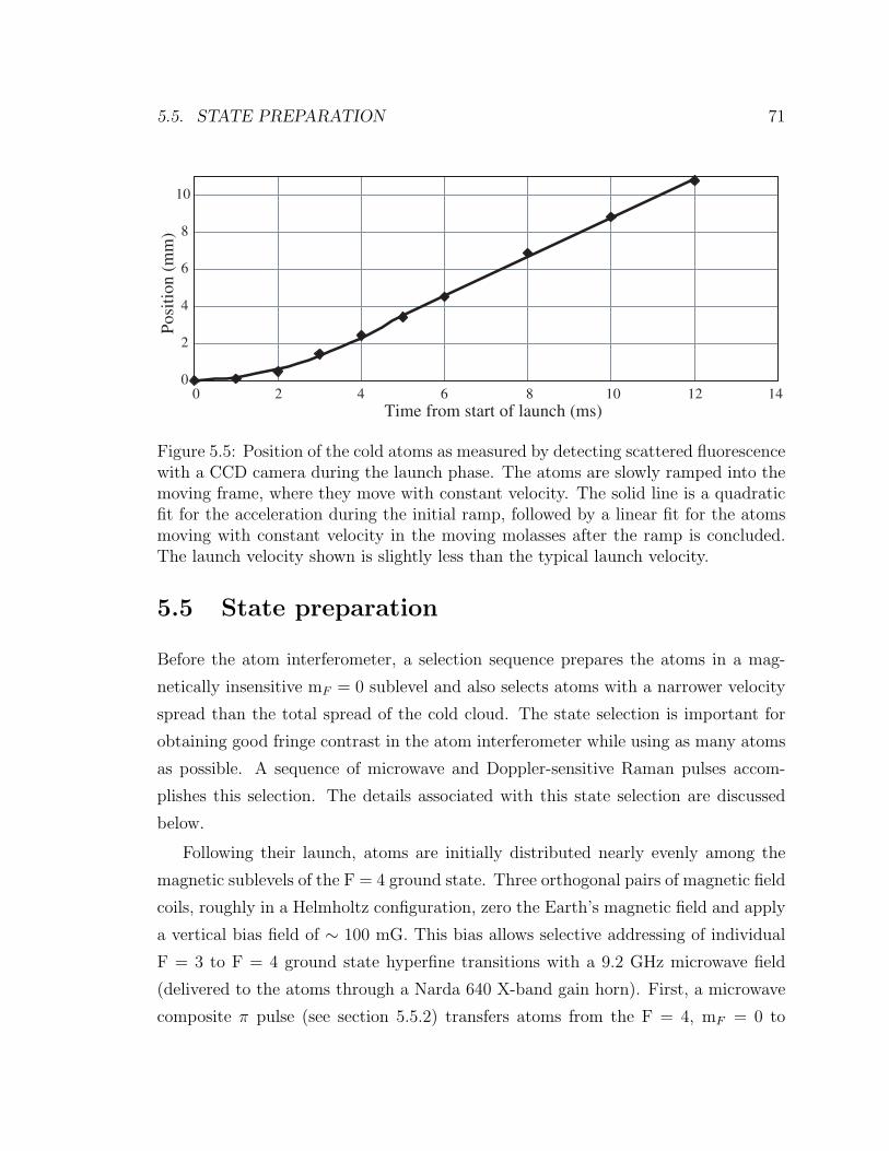
5.5. STATE PREPARATION 71
0
2
4
6
8
10
10 12 14
Pos
itio
n (m
m)
Time from start of launch (ms)0 2 4 6 8
Figure 5.5: Position of the cold atoms as measured by detecting scattered fluorescencewith a CCD camera during the launch phase. The atoms are slowly ramped into themoving frame, where they move with constant velocity. The solid line is a quadraticfit for the acceleration during the initial ramp, followed by a linear fit for the atomsmoving with constant velocity in the moving molasses after the ramp is concluded.The launch velocity shown is slightly less than the typical launch velocity.
5.5 State preparation
Before the atom interferometer, a selection sequence prepares the atoms in a mag-
netically insensitive mF = 0 sublevel and also selects atoms with a narrower velocity
spread than the total spread of the cold cloud. The state selection is important for
obtaining good fringe contrast in the atom interferometer while using as many atoms
as possible. A sequence of microwave and Doppler-sensitive Raman pulses accom-
plishes this selection. The details associated with this state selection are discussed
below.
Following their launch, atoms are initially distributed nearly evenly among the
magnetic sublevels of the F = 4 ground state. Three orthogonal pairs of magnetic field
coils, roughly in a Helmholtz configuration, zero the Earth’s magnetic field and apply
a vertical bias field of ∼ 100 mG. This bias allows selective addressing of individual
F = 3 to F = 4 ground state hyperfine transitions with a 9.2 GHz microwave field
(delivered to the atoms through a Narda 640 X-band gain horn). First, a microwave
composite π pulse (see section 5.5.2) transfers atoms from the F = 4, mF = 0 to
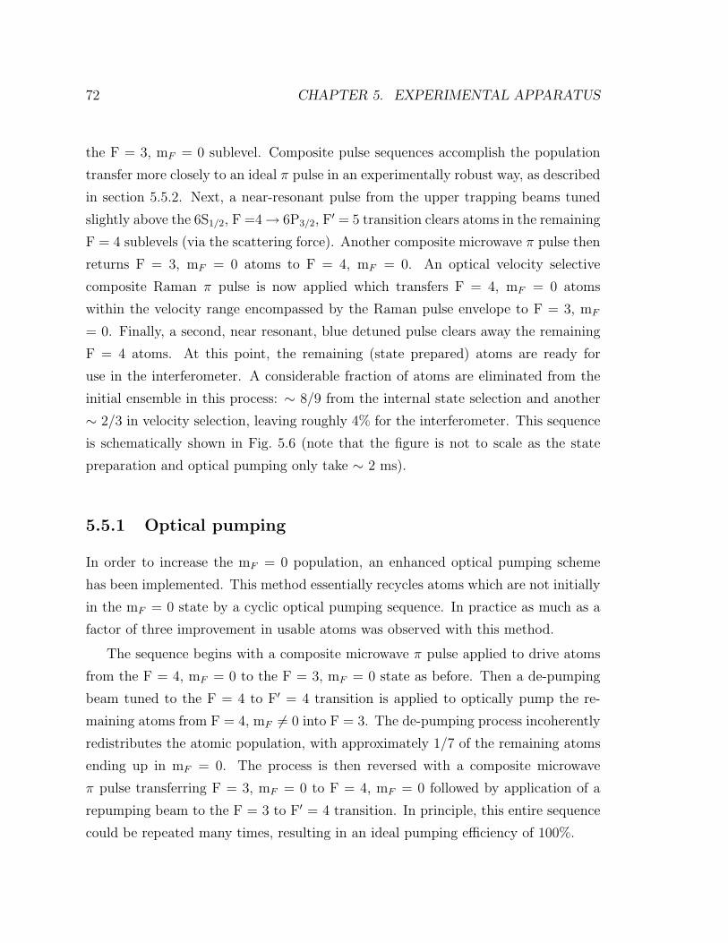
72 CHAPTER 5. EXPERIMENTAL APPARATUS
the F = 3, mF = 0 sublevel. Composite pulse sequences accomplish the population
transfer more closely to an ideal π pulse in an experimentally robust way, as described
in section 5.5.2. Next, a near-resonant pulse from the upper trapping beams tuned
slightly above the 6S1/2, F =4 → 6P3/2, F′ = 5 transition clears atoms in the remaining
F = 4 sublevels (via the scattering force). Another composite microwave π pulse then
returns F = 3, mF = 0 atoms to F = 4, mF = 0. An optical velocity selective
composite Raman π pulse is now applied which transfers F = 4, mF = 0 atoms
within the velocity range encompassed by the Raman pulse envelope to F = 3, mF
= 0. Finally, a second, near resonant, blue detuned pulse clears away the remaining
F = 4 atoms. At this point, the remaining (state prepared) atoms are ready for
use in the interferometer. A considerable fraction of atoms are eliminated from the
initial ensemble in this process: ∼ 8/9 from the internal state selection and another
∼ 2/3 in velocity selection, leaving roughly 4% for the interferometer. This sequence
is schematically shown in Fig. 5.6 (note that the figure is not to scale as the state
preparation and optical pumping only take ∼ 2 ms).
5.5.1 Optical pumping
In order to increase the mF = 0 population, an enhanced optical pumping scheme
has been implemented. This method essentially recycles atoms which are not initially
in the mF = 0 state by a cyclic optical pumping sequence. In practice as much as a
factor of three improvement in usable atoms was observed with this method.
The sequence begins with a composite microwave π pulse applied to drive atoms
from the F = 4, mF = 0 to the F = 3, mF = 0 state as before. Then a de-pumping
beam tuned to the F = 4 to F′ = 4 transition is applied to optically pump the re-
maining atoms from F = 4, mF = 0 into F = 3. The de-pumping process incoherently
redistributes the atomic population, with approximately 1/7 of the remaining atoms
ending up in mF = 0. The process is then reversed with a composite microwave
π pulse transferring F = 3, mF = 0 to F = 4, mF = 0 followed by application of a
repumping beam to the F = 3 to F′ = 4 transition. In principle, this entire sequence
could be repeated many times, resulting in an ideal pumping efficiency of 100%.
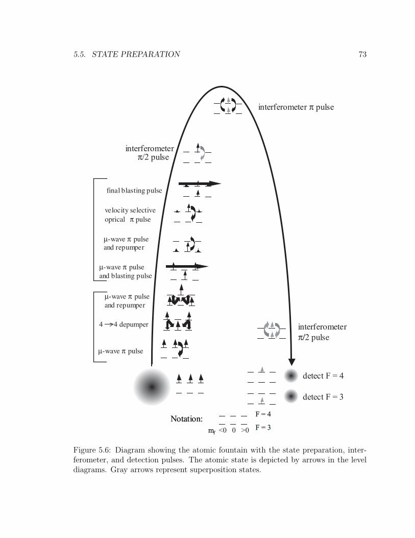
5.5. STATE PREPARATION 73
Notation:F = 4
F = 3mf <0 0 >0
Notation:F = 4
F = 3mf
µ-wave π pulse and blasting pulse
µ-wave π pulse
4 4 depumper
µ-wave π pulse and repumper
velocity selectiveoprical π pulse
µ-wave π pulse and repumper
final blasting pulse
interferometer π/2 pulse
interferometer π pulse
interferometer π/2 pulse
detect F = 4
detect F = 3
Figure 5.6: Diagram showing the atomic fountain with the state preparation, inter-ferometer, and detection pulses. The atomic state is depicted by arrows in the leveldiagrams. Gray arrows represent superposition states.
74 CHAPTER 5. EXPERIMENTAL APPARATUS
In practice, inefficiency of the microwave pulses (see section 5.5.2), heating due to
spontaneous emission in the pumping sequence, and the availability of only a finite
amount of time to execute the sequence limit the process efficiency. We realize a factor
of three improvement with just one cycle of the sequence described in the previous
paragraph.
For vapor cell loaded traps there is another effect which limits the overall efficiency
by the presence of the background atomic vapor. In this case, the de-pumping photons
can excite atoms in the background vapor which then can emit light at the repumping
frequency as they spontaneously decay. These rescattered photons then redistribute
atoms in the F = 3, mF = 0 state to other mF = 0 states. Thus there is a trade-
off between background vapor pressure (which sets the loading rate) and the overall
efficiency of the pumping scheme (which works best at low vapor pressure). For the
operating parameters of this experiment, the optical pumping typically improves the
usable number of atoms by a factor of 1.5 - 2. Finally, it is noted that this method
substantially increases shot-to-shot atom number fluctuations (from 200:1 to 60:1).
However, the normalized detection method is able to effectively suppress the impact
of these fluctuations on the interferometer signals. It is not understood what drives
the increased noise.
5.5.2 Composite pulse techniques
The above state preparation methods work best with efficient coherent population
transfer between F = 3 and F = 4 states. Less than unit transfer efficiency during
a standard π pulse between the ground states can result from an inhomogeneous
Rabi frequency of the microwave or optical pulse seen by the atoms, as well as by
detunings due to the velocity spread of the atoms. In this apparatus, the microwave
π pulses are typically only 80% efficient due to inhomogeneous field strengths across
the atom clouds (since the microwave transitions are driven with horns placed outside
the vacuum chamber). Furthermore, the state selection and optical pumping require
a series of one optical and four microwave π pulses in the two separate chambers.
With the current system, it is difficult to match the pulse conditions for all pairs of
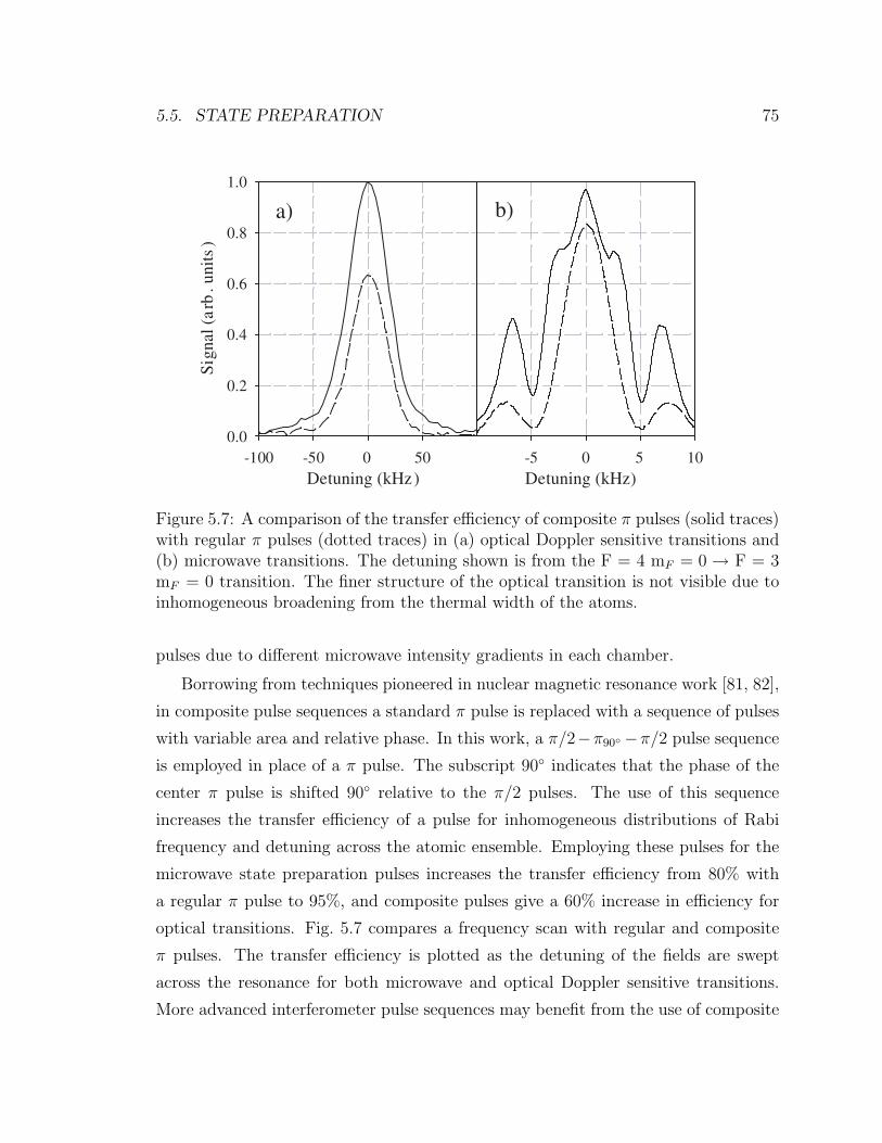
5.5. STATE PREPARATION 75
Detuning (kHz)-100 -50 0 50
Sig
nal (
arb
. uni
ts)
0.0
0.2
0.4
0.6
0.8
1.0
Detuning (kHz)-5 0 5 10
a) b)
Figure 5.7: A comparison of the transfer efficiency of composite π pulses (solid traces)with regular π pulses (dotted traces) in (a) optical Doppler sensitive transitions and(b) microwave transitions. The detuning shown is from the F = 4 mF = 0 → F = 3mF = 0 transition. The finer structure of the optical transition is not visible due toinhomogeneous broadening from the thermal width of the atoms.
pulses due to different microwave intensity gradients in each chamber.
Borrowing from techniques pioneered in nuclear magnetic resonance work [81, 82],
in composite pulse sequences a standard π pulse is replaced with a sequence of pulses
with variable area and relative phase. In this work, a π/2−π90 −π/2 pulse sequence
is employed in place of a π pulse. The subscript 90 indicates that the phase of the
center π pulse is shifted 90 relative to the π/2 pulses. The use of this sequence
increases the transfer efficiency of a pulse for inhomogeneous distributions of Rabi
frequency and detuning across the atomic ensemble. Employing these pulses for the
microwave state preparation pulses increases the transfer efficiency from 80% with
a regular π pulse to 95%, and composite pulses give a 60% increase in efficiency for
optical transitions. Fig. 5.7 compares a frequency scan with regular and composite
π pulses. The transfer efficiency is plotted as the detuning of the fields are swept
across the resonance for both microwave and optical Doppler sensitive transitions.
More advanced interferometer pulse sequences may benefit from the use of composite
76 CHAPTER 5. EXPERIMENTAL APPARATUS
pulses for the optical pulses (see Fig. 5.7) but are not employed at the moment (see
section 7.2.2).
In comparison with the adiabatic rapid passage technique (ARP), where the de-
tuning of the laser is swept across the resonance rapidly so that the state vector
follows adiabatically [51], composite pulses are easier to implement experimentally
and require less time (or total pulse area) to achieve efficient transfer. For example,
it is found that approximately 5π total time (here time is referenced to the time to
drive a π pulse at the resonant Rabi frequency) is needed for ARP to achieve results
similar to those achieved with only 2π time for the composite sequence. Addition-
ally, ARP gives significantly more spontaneous emission for optical pulses due to the
increased length.
5.6 Atom interferometer
This section describes the operation of the atom interferometer and the directly re-
lated subsystems. The generation of the Raman lasers is detailed, as well as their
delivery to the atoms. A technique to remove systematics based on the reversal of
the propagation vector of the Raman beams is presented. The rationale behind the
specific Raman beam operating parameters is discussed. Finally, the operation of the
interferometer itself is described.
5.6.1 Raman lasers
As the acceleration-induced phase shifts depend critically on the phase and wavevector
associated with the laser beams used to drive stimulated Raman transitions, possible
contributions of laser frequency noise to the relative stabilities of the interferometer
signals is analyzed. The constraints on laser frequency stability are considered here,
and then the Raman laser system which was designed to meet these constraints is
described.
In the gradiometer geometry, the two ensembles are separated by ∼ 1.4 m. The
Raman fields propagate in an asymmetric way to these ensembles as seen in Fig. 5.8.
5.6. ATOM INTERFEROMETER 77
The rationale behind the asymmetric design is given in section 5.6.2. Consider the
propagation paths of the optical fields following the beamsplitting optic which sepa-
rates the two Raman fields. The beam of frequency ω1 propagates roughly x11 0.3 m
before it passes through the first ensemble of atoms, while it propagates roughly x21 1.7 m before it passes through the second ensemble. On the other hand, the beam of
frequency ω2 propagates x12 3.7 m before it passes through the first ensemble, while
it propagates x22 2.3 m before it passes through the second ensemble.
If the laser frequencies drift on a time scale short compared to the interrogation
time T between pulses, an asymmetric phase shift will be read into the atomic coher-
ences due to this path asymmetry. For example, suppose the laser frequency jitter
is δω, while the differential path length travelled by the Raman lasers for the two
ensembles is
0 ≡ (effective path to ensemble 1) − (effective path to ensemble 2)
= (x12 − x11) − (x22 − x21) 2.8m. (5.1)
This frequency noise leads to differential phase noise of δφlaser ∼ (k0)(δω/ω). For a
target interference SNR of 1000:1, δφlaser < 1 mrad. For our parameters, this implies
δω < 2π × 20 kHz.
In order to achieve frequency stability at this level, a second Vortex laser is used
as the master laser for the Raman laser system. This laser is locked to the 6S1/2, F
= 3 → 6P3/2, F′ = 2 crossover resonance (also via modulation transfer spectroscopy)
using several AOMs to offset the frequency to obtain the desired Raman detuning.
The lock is maintained through the use of a digital signal processor (DSP, Spectrum
Signal Indy TMS320C32). The DSP processes the lock error signal through a highpass
and lowpass channel, each operating at a sampling rate of 25 kHz. The high and low
frequency channels are divided to provide feedback to the laser current and to the
cavity piezo element respectively. Due to the presence of long term drift in the piezo
element a third, very low frequency channel is provided through a GPIB command
to the laser controller, which allows the laser to stay locked over several days. The
measured stability of the laser is comparable to that of the master laser used for
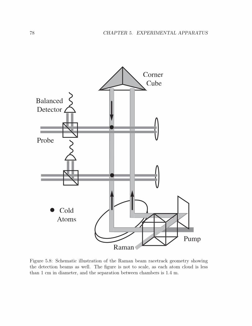
78 CHAPTER 5. EXPERIMENTAL APPARATUS
BalancedDetector
Corner Cube
RamanRamanPump
Probe
ColdAtoms
Figure 5.8: Schematic illustration of the Raman beam racetrack geometry showingthe detection beams as well. The figure is not to scale, as each atom cloud is lessthan 1 cm in diameter, and the separation between chambers is 1.4 m.
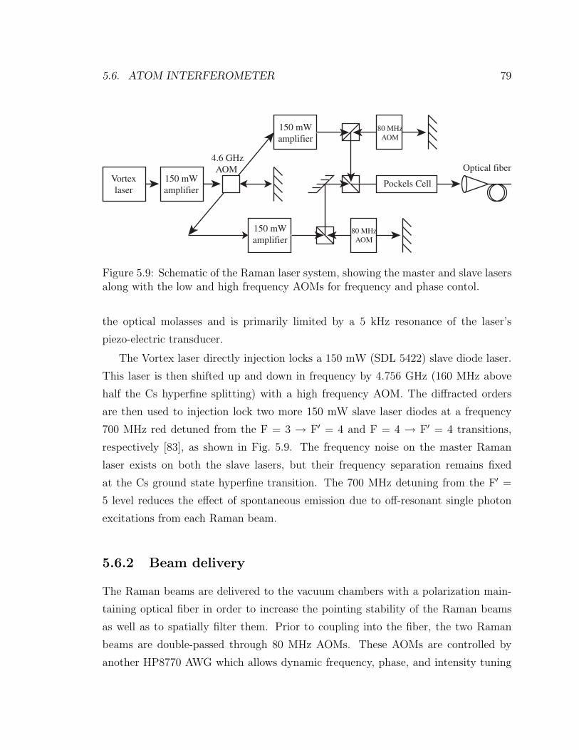
5.6. ATOM INTERFEROMETER 79
4.6 GHz AOM
150 mWamplifier
150 mWamplifier
80 MHzAOM
80 MHzAOM
Pockels Cell
Optical fiber150 mWamplifier
Vortexlaser
Figure 5.9: Schematic of the Raman laser system, showing the master and slave lasersalong with the low and high frequency AOMs for frequency and phase contol.
the optical molasses and is primarily limited by a 5 kHz resonance of the laser’s
piezo-electric transducer.
The Vortex laser directly injection locks a 150 mW (SDL 5422) slave diode laser.
This laser is then shifted up and down in frequency by 4.756 GHz (160 MHz above
half the Cs hyperfine splitting) with a high frequency AOM. The diffracted orders
are then used to injection lock two more 150 mW slave laser diodes at a frequency
700 MHz red detuned from the F = 3 → F′ = 4 and F = 4 → F′ = 4 transitions,
respectively [83], as shown in Fig. 5.9. The frequency noise on the master Raman
laser exists on both the slave lasers, but their frequency separation remains fixed
at the Cs ground state hyperfine transition. The 700 MHz detuning from the F′ =
5 level reduces the effect of spontaneous emission due to off-resonant single photon
excitations from each Raman beam.
5.6.2 Beam delivery
The Raman beams are delivered to the vacuum chambers with a polarization main-
taining optical fiber in order to increase the pointing stability of the Raman beams
as well as to spatially filter them. Prior to coupling into the fiber, the two Raman
beams are double-passed through 80 MHz AOMs. These AOMs are controlled by
another HP8770 AWG which allows dynamic frequency, phase, and intensity tuning
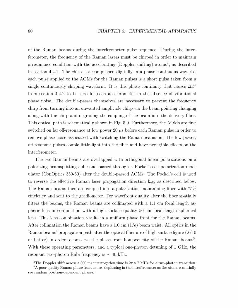
80 CHAPTER 5. EXPERIMENTAL APPARATUS
of the Raman beams during the interferometer pulse sequence. During the inter-
ferometer, the frequency of the Raman lasers must be chirped in order to maintain
a resonance condition with the accelerating (Doppler shifting) atoms4, as described
in section 4.4.1. The chirp is accomplished digitally in a phase-continuous way, i.e.
each pulse applied to the AOMs for the Raman pulses is a short pulse taken from a
single continuously chirping waveform. It is this phase continuity that causes ∆φ
from section 4.4.2 to be zero for each accelerometer in the absence of vibrational
phase noise. The double-passes themselves are necessary to prevent the frequency
chirp from turning into an unwanted amplitude chirp via the beam pointing changing
along with the chirp and degrading the coupling of the beam into the delivery fiber.
This optical path is schematically shown in Fig. 5.9. Furthermore, the AOMs are first
switched on far off-resonance at low power 20 µs before each Raman pulse in order to
remove phase noise associated with switching the Raman beams on. The low power,
off-resonant pulses couple little light into the fiber and have negligible effects on the
interferometer.
The two Raman beams are overlapped with orthogonal linear polarizations on a
polarizing beamsplitting cube and passed through a Pockel’s cell polarization mod-
ulator (ConOptics 350-50) after the double-passed AOMs. The Pockel’s cell is used
to reverse the effective Raman laser propagation direction keff, as described below.
The Raman beams then are coupled into a polarization maintaining fiber with 75%
efficiency and sent to the gradiometer. For wavefront quality after the fiber spatially
filters the beams, the Raman beams are collimated with a 1.1 cm focal length as-
pheric lens in conjunction with a high surface quality 50 cm focal length spherical
lens. This lens combination results in a uniform phase front for the Raman beams.
After collimation the Raman beams have a 1.0 cm (1/e) beam waist. All optics in the
Raman beams’ propagation path after the optical fiber are of high surface figure (λ/10
or better) in order to preserve the phase front homogeneity of the Raman beams5.
With these operating parameters, and a typical one-photon detuning of 1 GHz, the
resonant two-photon Rabi frequency is ∼ 40 kHz.
4The Doppler shift across a 300 ms interrogation time is 2π×7 MHz for a two-photon transition.5A poor quality Raman phase front causes dephasing in the interferometer as the atoms essentially
see random position-dependent phases.
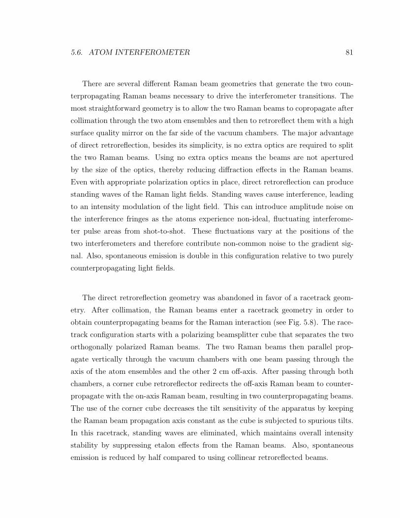
5.6. ATOM INTERFEROMETER 81
There are several different Raman beam geometries that generate the two coun-
terpropagating Raman beams necessary to drive the interferometer transitions. The
most straightforward geometry is to allow the two Raman beams to copropagate after
collimation through the two atom ensembles and then to retroreflect them with a high
surface quality mirror on the far side of the vacuum chambers. The major advantage
of direct retroreflection, besides its simplicity, is no extra optics are required to split
the two Raman beams. Using no extra optics means the beams are not apertured
by the size of the optics, thereby reducing diffraction effects in the Raman beams.
Even with appropriate polarization optics in place, direct retroreflection can produce
standing waves of the Raman light fields. Standing waves cause interference, leading
to an intensity modulation of the light field. This can introduce amplitude noise on
the interference fringes as the atoms experience non-ideal, fluctuating interferome-
ter pulse areas from shot-to-shot. These fluctuations vary at the positions of the
two interferometers and therefore contribute non-common noise to the gradient sig-
nal. Also, spontaneous emission is double in this configuration relative to two purely
counterpropagating light fields.
The direct retroreflection geometry was abandoned in favor of a racetrack geom-
etry. After collimation, the Raman beams enter a racetrack geometry in order to
obtain counterpropagating beams for the Raman interaction (see Fig. 5.8). The race-
track configuration starts with a polarizing beamsplitter cube that separates the two
orthogonally polarized Raman beams. The two Raman beams then parallel prop-
agate vertically through the vacuum chambers with one beam passing through the
axis of the atom ensembles and the other 2 cm off-axis. After passing through both
chambers, a corner cube retroreflector redirects the off-axis Raman beam to counter-
propagate with the on-axis Raman beam, resulting in two counterpropagating beams.
The use of the corner cube decreases the tilt sensitivity of the apparatus by keeping
the Raman beam propagation axis constant as the cube is subjected to spurious tilts.
In this racetrack, standing waves are eliminated, which maintains overall intensity
stability by suppressing etalon effects from the Raman beams. Also, spontaneous
emission is reduced by half compared to using collinear retroreflected beams.
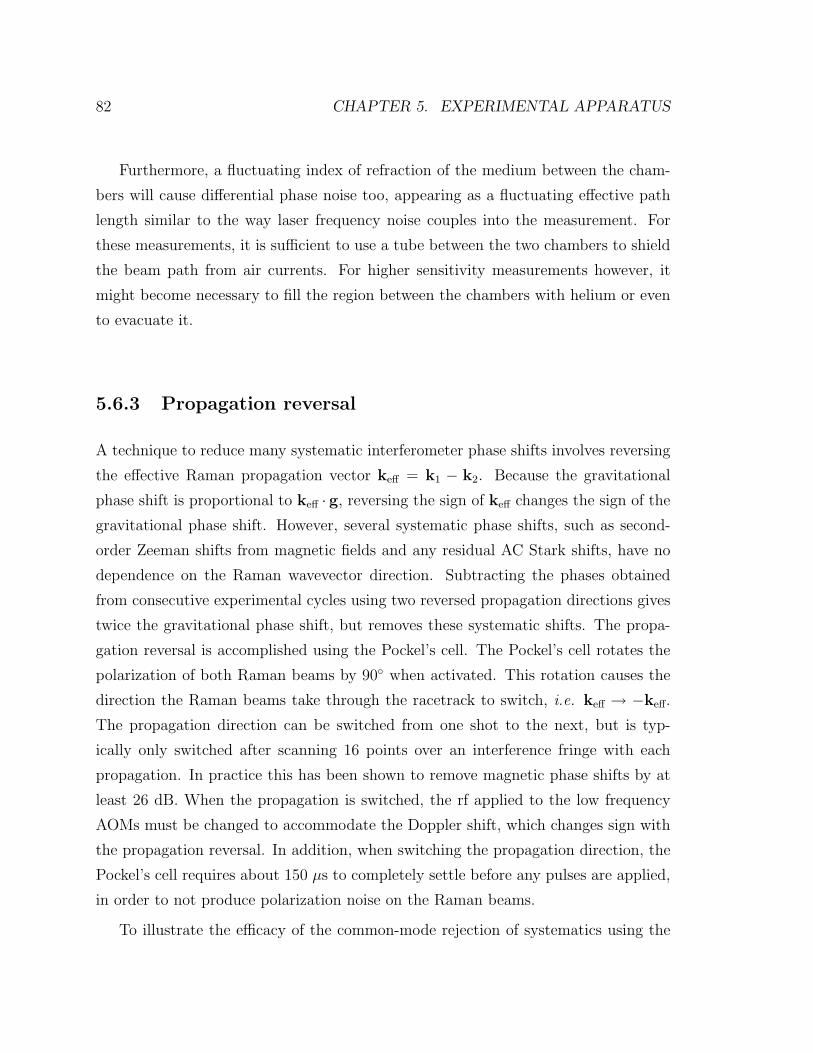
82 CHAPTER 5. EXPERIMENTAL APPARATUS
Furthermore, a fluctuating index of refraction of the medium between the cham-
bers will cause differential phase noise too, appearing as a fluctuating effective path
length similar to the way laser frequency noise couples into the measurement. For
these measurements, it is sufficient to use a tube between the two chambers to shield
the beam path from air currents. For higher sensitivity measurements however, it
might become necessary to fill the region between the chambers with helium or even
to evacuate it.
5.6.3 Propagation reversal
A technique to reduce many systematic interferometer phase shifts involves reversing
the effective Raman propagation vector keff = k1 − k2. Because the gravitational
phase shift is proportional to keff · g, reversing the sign of keff changes the sign of the
gravitational phase shift. However, several systematic phase shifts, such as second-
order Zeeman shifts from magnetic fields and any residual AC Stark shifts, have no
dependence on the Raman wavevector direction. Subtracting the phases obtained
from consecutive experimental cycles using two reversed propagation directions gives
twice the gravitational phase shift, but removes these systematic shifts. The propa-
gation reversal is accomplished using the Pockel’s cell. The Pockel’s cell rotates the
polarization of both Raman beams by 90 when activated. This rotation causes the
direction the Raman beams take through the racetrack to switch, i.e. keff → −keff.
The propagation direction can be switched from one shot to the next, but is typ-
ically only switched after scanning 16 points over an interference fringe with each
propagation. In practice this has been shown to remove magnetic phase shifts by at
least 26 dB. When the propagation is switched, the rf applied to the low frequency
AOMs must be changed to accommodate the Doppler shift, which changes sign with
the propagation reversal. In addition, when switching the propagation direction, the
Pockel’s cell requires about 150 µs to completely settle before any pulses are applied,
in order to not produce polarization noise on the Raman beams.
To illustrate the efficacy of the common-mode rejection of systematics using the
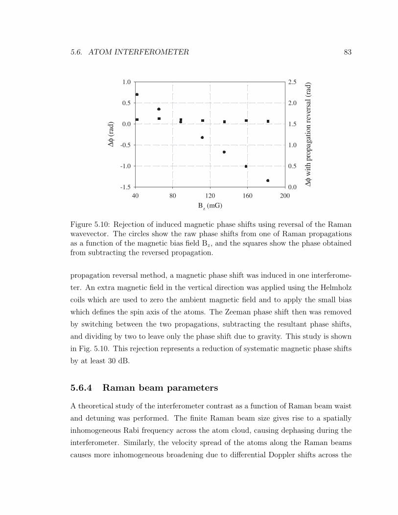
5.6. ATOM INTERFEROMETER 83
Bz (mG)40 80 120 160 200
∆φ (
rad)
-1.5
-1.0
-0.5
0.0
0.5
1.0
∆φ w
ith p
ropa
gatio
n re
vers
al (
rad)
0.0
0.5
1.0
1.5
2.0
2.5
Figure 5.10: Rejection of induced magnetic phase shifts using reversal of the Ramanwavevector. The circles show the raw phase shifts from one of Raman propagationsas a function of the magnetic bias field Bz, and the squares show the phase obtainedfrom subtracting the reversed propagation.
propagation reversal method, a magnetic phase shift was induced in one interferome-
ter. An extra magnetic field in the vertical direction was applied using the Helmholz
coils which are used to zero the ambient magnetic field and to apply the small bias
which defines the spin axis of the atoms. The Zeeman phase shift then was removed
by switching between the two propagations, subtracting the resultant phase shifts,
and dividing by two to leave only the phase shift due to gravity. This study is shown
in Fig. 5.10. This rejection represents a reduction of systematic magnetic phase shifts
by at least 30 dB.
5.6.4 Raman beam parameters
A theoretical study of the interferometer contrast as a function of Raman beam waist
and detuning was performed. The finite Raman beam size gives rise to a spatially
inhomogeneous Rabi frequency across the atom cloud, causing dephasing during the
interferometer. Similarly, the velocity spread of the atoms along the Raman beams
causes more inhomogeneous broadening due to differential Doppler shifts across the
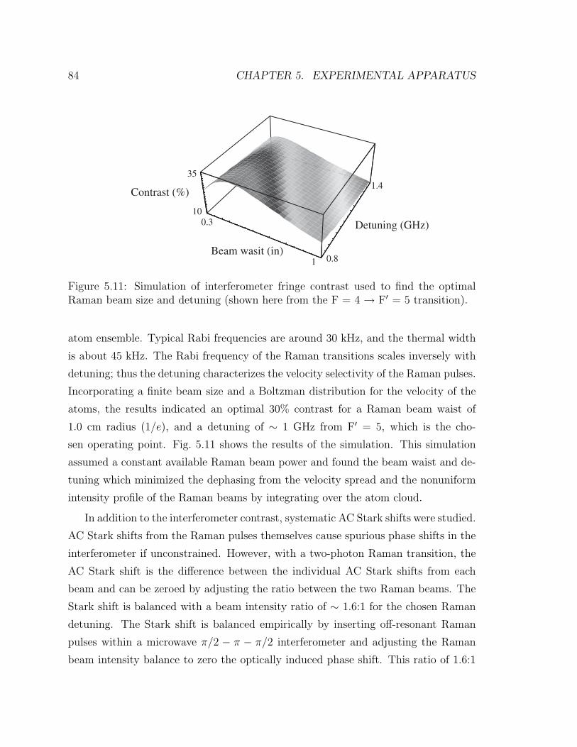
84 CHAPTER 5. EXPERIMENTAL APPARATUS
Detuning (GHz)
Beam wasit (in)
Contrast (%)
10
35
0.8
1.4
1
0.3
Figure 5.11: Simulation of interferometer fringe contrast used to find the optimalRaman beam size and detuning (shown here from the F = 4 → F′ = 5 transition).
atom ensemble. Typical Rabi frequencies are around 30 kHz, and the thermal width
is about 45 kHz. The Rabi frequency of the Raman transitions scales inversely with
detuning; thus the detuning characterizes the velocity selectivity of the Raman pulses.
Incorporating a finite beam size and a Boltzman distribution for the velocity of the
atoms, the results indicated an optimal 30% contrast for a Raman beam waist of
1.0 cm radius (1/e), and a detuning of ∼ 1 GHz from F′ = 5, which is the cho-
sen operating point. Fig. 5.11 shows the results of the simulation. This simulation
assumed a constant available Raman beam power and found the beam waist and de-
tuning which minimized the dephasing from the velocity spread and the nonuniform
intensity profile of the Raman beams by integrating over the atom cloud.
In addition to the interferometer contrast, systematic AC Stark shifts were studied.
AC Stark shifts from the Raman pulses themselves cause spurious phase shifts in the
interferometer if unconstrained. However, with a two-photon Raman transition, the
AC Stark shift is the difference between the individual AC Stark shifts from each
beam and can be zeroed by adjusting the ratio between the two Raman beams. The
Stark shift is balanced with a beam intensity ratio of ∼ 1.6:1 for the chosen Raman
detuning. The Stark shift is balanced empirically by inserting off-resonant Raman
pulses within a microwave π/2 − π − π/2 interferometer and adjusting the Raman
beam intensity balance to zero the optically induced phase shift. This ratio of 1.6:1
5.7. DETECTION SYSTEM 85
for the chosen Raman detuning agrees well with theoretical predictions.
5.6.5 Interferometer operation
The gradiometer is typically operated in its most sensitive configuration with the
interferometer pulses at a spacing of T = 150 ms. The interferometer time can be
lengthened to as much as T = 157.5 ms, but care must be taken to avoid driving
transitions at the apex of the atomic fountain. At this point, the atoms have zero
velocity, and Doppler sensitive transitions are degenerate with Doppler insensitive
transitions which can be driven due to small amounts of polarization impurity in the
Raman beams. The maximum interferometer time is limited by the vacuum cham-
ber size which constrains the fountain height to 12 cm. Following the three-pulse
interferometer sequence, the population distribution of the atoms in each ensemble is
measured using the method described in section 5.7. In order to obtain interference
fringes and extract the gravitationally-induced phase shift, the phase of an interfer-
ometer pulse needs to be scanned. The scanning is accomplished digitally with the
AWG by scanning the phase of the rf waveform applied to the low frequency AOMs
in the Raman beam paths. Any of the pulses can be scanned to produce fringes; typ-
ically the first pulse is scanned. This phase scanning is in addition to the frequency
chirp to counteract the Doppler shift applied during the pulse. Typically the phase
is scanned over 2π rad in 16 points. The number of points is kept small to limit drift
of signal amplitude and fringe contrast. Within a period shorter than the drift time,
the length of a scan is not important, as the noise behaves as a white noise source.
5.7 Detection system
5.7.1 Background
In order to realize a sensitive gravity gradiometer, the atoms must be detected with
high precision following the interferometer. Standard techniques for atom detection
include measuring scattered fluorescence or absorption. Both these techniques require
careful stabilization of the amplitude and frequency of the probe light to achieve a high
86 CHAPTER 5. EXPERIMENTAL APPARATUS
SNR. Fluorescence detection can be hampered by significant scattered light from the
background thermal vapor, although it can achieve quantum projection (shot noise)
limited performance under the right conditions [84]. In this experiment fluorescence
detection of cold atoms was limited to a SNR of 300:1 by photon shot-noise from light
scattered by background atoms in the vapor-cell trap due to the small solid angle of of
light scattered by the cold atoms collected by the detection system. Using FM probe
light in fluorescence detection suppresses the background signal, but does not improve
the photon shot-noise limited SNR. Using absorption of the probe beam effectively
collects the entire amount of light scattered from the cold atoms and overcomes this
noise source. However, due to the large background of unabsorbed light, absorption
detection places very tight constraints on probe amplitude and frequency stability.
Use of a FM probe (in a Pound-Drever-Hall configuration [85]) eases these constraints,
but residual amplitude modulation6 (RAM) at the 10−5 level limited the SNR to 100:1.
In order to overcome these limits, a balanced, modulation transfer detection system
was designed to eliminate background vapor noise as well as to maximize the SNR
limit from the cold atoms.
Balanced detection makes use of the fact that the experiment requires detection
of atoms in a coherent superposition of two internal atomic states following an atom
interferometer, i.e. detection of population differences. Common-mode suppression
of technical noise sources arising from laser amplitude and frequency noise is made
possible by detecting population differences. In the method described below, fol-
lowing the interferometer, the two states are spatially separated using light induced
forces, which also projects the coherent superposition onto a statistical mixture of
atoms in each of the two states. After the spatial separation, the absorption of two
near resonant probe beams (each derived from the same laser) is measured on a bal-
anced photodetector (where the photocurrents from two matched photodiodes are
subtracted before amplification). In the case of equal populations between the two
atomic states, this simultaneous differential detection produces a null signal, with
high immunity to frequency or intensity noise from the laser.
6Residual amplitude modulation occurs due to etalon effects affecting the frequency modulatedsidebands differentially, leading to amplitude modulation.
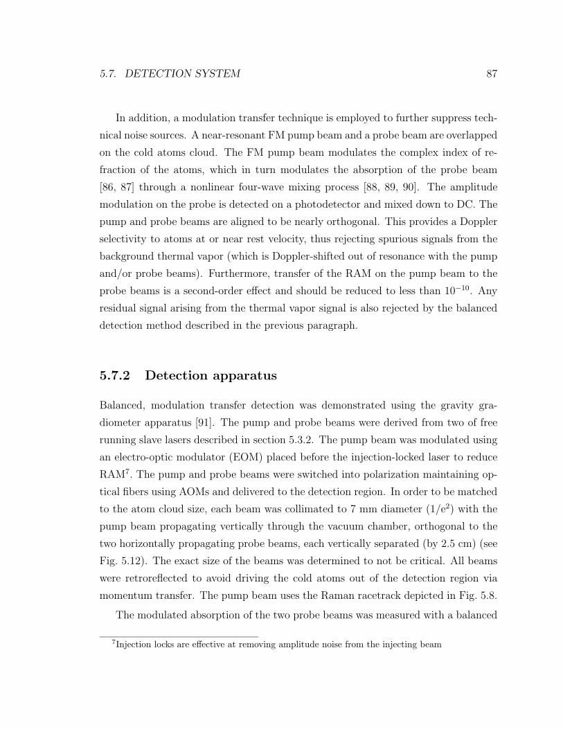
5.7. DETECTION SYSTEM 87
In addition, a modulation transfer technique is employed to further suppress tech-
nical noise sources. A near-resonant FM pump beam and a probe beam are overlapped
on the cold atoms cloud. The FM pump beam modulates the complex index of re-
fraction of the atoms, which in turn modulates the absorption of the probe beam
[86, 87] through a nonlinear four-wave mixing process [88, 89, 90]. The amplitude
modulation on the probe is detected on a photodetector and mixed down to DC. The
pump and probe beams are aligned to be nearly orthogonal. This provides a Doppler
selectivity to atoms at or near rest velocity, thus rejecting spurious signals from the
background thermal vapor (which is Doppler-shifted out of resonance with the pump
and/or probe beams). Furthermore, transfer of the RAM on the pump beam to the
probe beams is a second-order effect and should be reduced to less than 10−10. Any
residual signal arising from the thermal vapor signal is also rejected by the balanced
detection method described in the previous paragraph.
5.7.2 Detection apparatus
Balanced, modulation transfer detection was demonstrated using the gravity gra-
diometer apparatus [91]. The pump and probe beams were derived from two of free
running slave lasers described in section 5.3.2. The pump beam was modulated using
an electro-optic modulator (EOM) placed before the injection-locked laser to reduce
RAM7. The pump and probe beams were switched into polarization maintaining op-
tical fibers using AOMs and delivered to the detection region. In order to be matched
to the atom cloud size, each beam was collimated to 7 mm diameter (1/e2) with the
pump beam propagating vertically through the vacuum chamber, orthogonal to the
two horizontally propagating probe beams, each vertically separated (by 2.5 cm) (see
Fig. 5.12). The exact size of the beams was determined to not be critical. All beams
were retroreflected to avoid driving the cold atoms out of the detection region via
momentum transfer. The pump beam uses the Raman racetrack depicted in Fig. 5.8.
The modulated absorption of the two probe beams was measured with a balanced
7Injection locks are effective at removing amplitude noise from the injecting beam
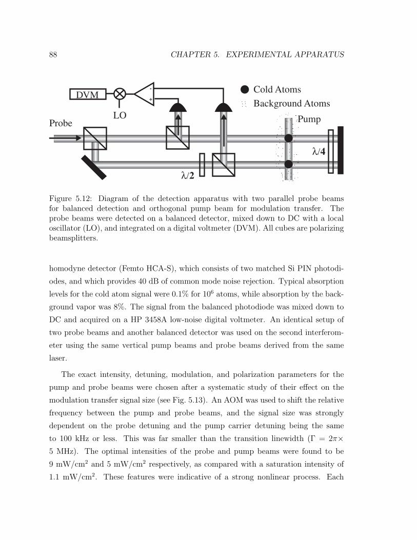
88 CHAPTER 5. EXPERIMENTAL APPARATUS
+
-
λ/4
λ/2
Probe Pump
Background Atoms
Cold Atoms
LO
DVM
Figure 5.12: Diagram of the detection apparatus with two parallel probe beamsfor balanced detection and orthogonal pump beam for modulation transfer. Theprobe beams were detected on a balanced detector, mixed down to DC with a localoscillator (LO), and integrated on a digital voltmeter (DVM). All cubes are polarizingbeamsplitters.
homodyne detector (Femto HCA-S), which consists of two matched Si PIN photodi-
odes, and which provides 40 dB of common mode noise rejection. Typical absorption
levels for the cold atom signal were 0.1% for 106 atoms, while absorption by the back-
ground vapor was 8%. The signal from the balanced photodiode was mixed down to
DC and acquired on a HP 3458A low-noise digital voltmeter. An identical setup of
two probe beams and another balanced detector was used on the second interferom-
eter using the same vertical pump beams and probe beams derived from the same
laser.
The exact intensity, detuning, modulation, and polarization parameters for the
pump and probe beams were chosen after a systematic study of their effect on the
modulation transfer signal size (see Fig. 5.13). An AOM was used to shift the relative
frequency between the pump and probe beams, and the signal size was strongly
dependent on the probe detuning and the pump carrier detuning being the same
to 100 kHz or less. This was far smaller than the transition linewidth (Γ = 2π×5 MHz). The optimal intensities of the probe and pump beams were found to be
9 mW/cm2 and 5 mW/cm2 respectively, as compared with a saturation intensity of
1.1 mW/cm2. These features were indicative of a strong nonlinear process. Each
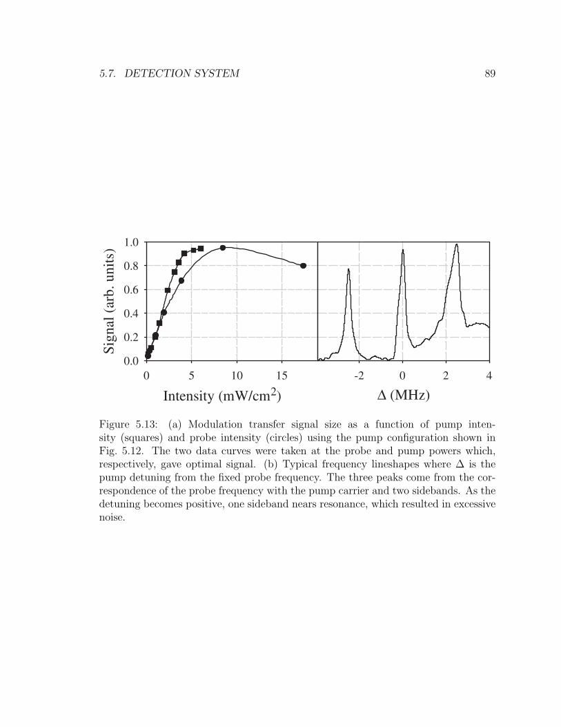
5.7. DETECTION SYSTEM 89
Intensity (mW/cm2)
0 5 10 15
Sign
al (
arb.
uni
ts)
0.0
0.2
0.4
0.6
0.8
1.0
∆ (MHz)-2 0 2 4
Figure 5.13: (a) Modulation transfer signal size as a function of pump inten-sity (squares) and probe intensity (circles) using the pump configuration shown inFig. 5.12. The two data curves were taken at the probe and pump powers which,respectively, gave optimal signal. (b) Typical frequency lineshapes where ∆ is thepump detuning from the fixed probe frequency. The three peaks come from the cor-respondence of the probe frequency with the pump carrier and two sidebands. As thedetuning becomes positive, one sideband nears resonance, which resulted in excessivenoise.
90 CHAPTER 5. EXPERIMENTAL APPARATUS
sideband contained 20% of the total power. The probe beams and the pump beam
carrier were detuned 6.5 MHz red of the 6S1/2, F = 4 → 6P3/2, F = 5 transition.
A 2.5 MHz modulation frequency was chosen based on theoretical predictions of
maximal signal with a modulation frequency of Γ/2 [86]; experimentally this value
was optimal as well. The optimum polarizations for the pump and probe beams were
σ+ and linear respectively.
The pump and probe beams had a kinetic effect on the cold atoms which could be
exploited to obtain long interrogation times. Because the beams were retroreflected
and red-detuned, they formed a two-dimensional optical molasses. The molasses
slowed and stopped atoms returning from the fountain while confining them along
the second axis as well. For this geometry, atoms in the 6S1/2, F = 4 state optically
pumped to the 6S1/2, F = 3 level via off-resonant excitations with a time constant of
4.6 ms. With the addition of a repumping beam, the time constant was extended to
16 ms, here limited by heating of atoms along the unconstrained axis. Alternatively,
the motion along all three axes could be constrained by using frequency modulated
molasses beams as the pump beams. In this configuration, detection times as long as
50 ms were achieved. However, in situations where there is significant phase noise,
such as in a gravimeter, it is not possible to remain centered on a fringe, and this
form of balanced detection with FM molasses beams is not suitable. More explicitly,
if the signal is not perfectly balanced, thereby rejecting fluctuations in atom number,
a different approach must be taken to remove the number fluctuations.
Using the pump configuration shown in Fig. 5.12, a two pulse detection sequence
was used in order to measure the total number of atoms as well as the difference
signal. First atoms in the F = 4 state were detected in the upper probe beam. These
atoms were stopped by a 2-D molasses consisting of the vertically oriented pump
beam and one of the horizontally oriented probe beams. Atoms in the F = 3 state
continued to fall. After 7 ms the F = 3 atoms were centered in the lower probe beam.
A repumper then pumped all atoms to the F = 4 state, and the differential signal was
detected. This signal consisted of the difference between the original F = 4 atoms
in the upper probe beam and the repumped F = 3 atoms in the lower. The total
atom number was inferred from a combination of the signals from the two detections
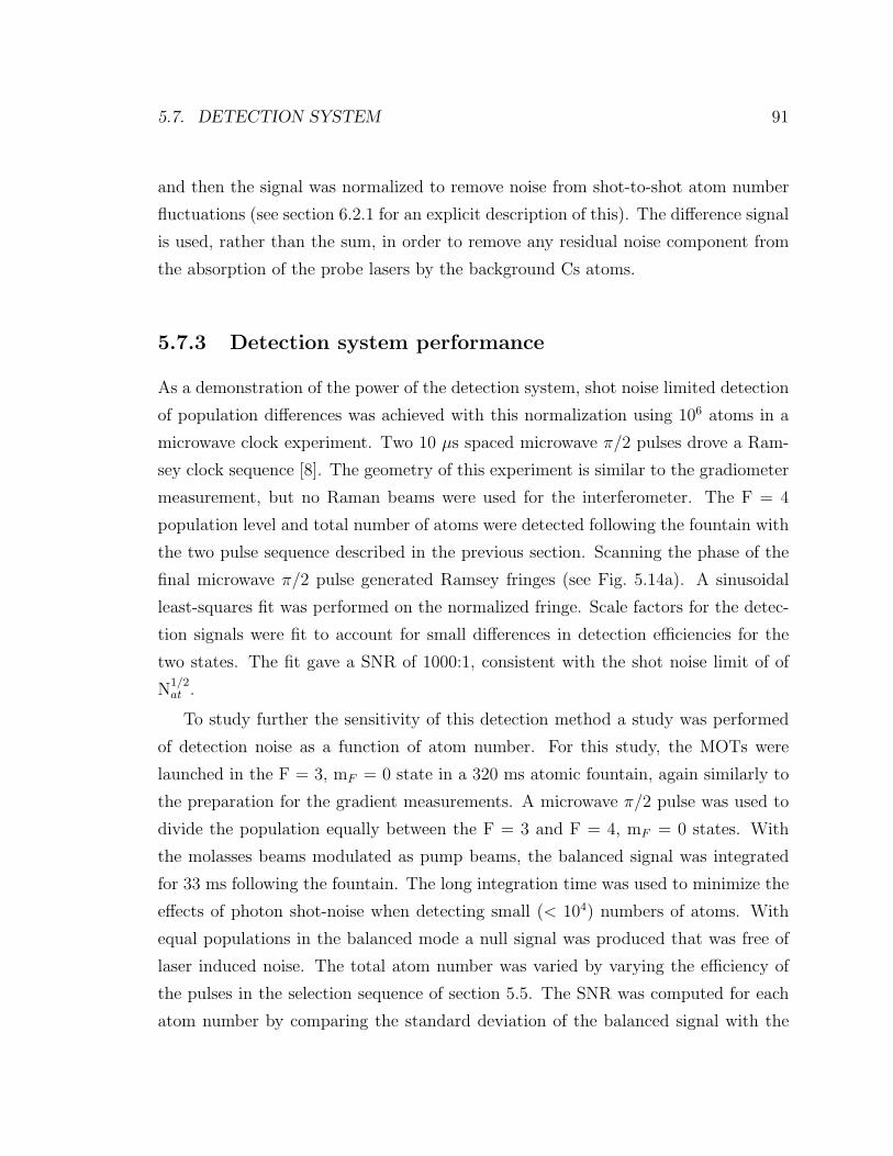
5.7. DETECTION SYSTEM 91
and then the signal was normalized to remove noise from shot-to-shot atom number
fluctuations (see section 6.2.1 for an explicit description of this). The difference signal
is used, rather than the sum, in order to remove any residual noise component from
the absorption of the probe lasers by the background Cs atoms.
5.7.3 Detection system performance
As a demonstration of the power of the detection system, shot noise limited detection
of population differences was achieved with this normalization using 106 atoms in a
microwave clock experiment. Two 10 µs spaced microwave π/2 pulses drove a Ram-
sey clock sequence [8]. The geometry of this experiment is similar to the gradiometer
measurement, but no Raman beams were used for the interferometer. The F = 4
population level and total number of atoms were detected following the fountain with
the two pulse sequence described in the previous section. Scanning the phase of the
final microwave π/2 pulse generated Ramsey fringes (see Fig. 5.14a). A sinusoidal
least-squares fit was performed on the normalized fringe. Scale factors for the detec-
tion signals were fit to account for small differences in detection efficiencies for the
two states. The fit gave a SNR of 1000:1, consistent with the shot noise limit of of
N1/2at .
To study further the sensitivity of this detection method a study was performed
of detection noise as a function of atom number. For this study, the MOTs were
launched in the F = 3, mF = 0 state in a 320 ms atomic fountain, again similarly to
the preparation for the gradient measurements. A microwave π/2 pulse was used to
divide the population equally between the F = 3 and F = 4, mF = 0 states. With
the molasses beams modulated as pump beams, the balanced signal was integrated
for 33 ms following the fountain. The long integration time was used to minimize the
effects of photon shot-noise when detecting small (< 104) numbers of atoms. With
equal populations in the balanced mode a null signal was produced that was free of
laser induced noise. The total atom number was varied by varying the efficiency of
the pulses in the selection sequence of section 5.5. The SNR was computed for each
atom number by comparing the standard deviation of the balanced signal with the
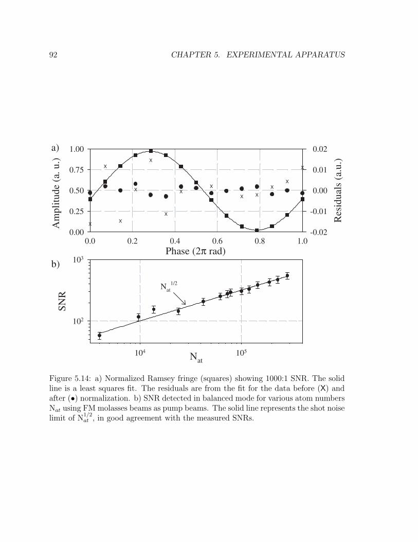
92 CHAPTER 5. EXPERIMENTAL APPARATUS
Phase (2π rad)0.0 0.2 0.4 0.6 0.8 1.0
Am
plitu
de (
a. u
.)
0.00
0.25
0.50
0.75
1.00
Res
idua
ls (
a.u.
)
-0.02
-0.01
0.00
0.01
0.02
X
X
X
X
X
X
X
XX
XX X
XX
X
a)
b)
Nat1/2
Nat104 105
SNR
102
103
Figure 5.14: a) Normalized Ramsey fringe (squares) showing 1000:1 SNR. The solidline is a least squares fit. The residuals are from the fit for the data before (X) andafter (•) normalization. b) SNR detected in balanced mode for various atom numbersNat using FM molasses beams as pump beams. The solid line represents the shot noiselimit of N
1/2at , in good agreement with the measured SNRs.
5.7. DETECTION SYSTEM 93
peak signal from all the atoms in one state (i.e. the maximally imbalanced signal).
The measured SNRs agree well with shot noise limited detection (N1/2at ) as shown in
Fig. 5.14b.
The peak performance of the modulation transfer method was exhibited with an
ensemble of ∼ 107 atoms, launched in the F = 4 state, but not state selected into
the mF = 0 sub-level. Normalizing the ensemble by detecting it with the two pulse
sequence yielded an SNR of 2350:1. Without normalization, the shot-to-shot atom
number fluctuations limited the SNR to 200:1.
Common-mode noise rejection ratios were measured for both laser amplitude and
frequency noise as well as atom number fluctuations by deliberately inducing these
noise sources. Balanced detection rejected these noise sources at the 40 dB, 24 dB
and 27 dB levels respectively. The laser amplitude noise rejection of 40 dB (dc -
10 MHz) was limited only by the balancing of the balanced photodiode pair. Fre-
quency noise rejection was characterized by driving high frequency noise at 2.5 kHz
during a shortened detection pulse8 as well as by making low frequency changes to
the pump and probe beams together in the balanced detection. Both tests showed
similar results. With this noise rejection, we inferred that atom shot noise limited
performance could be achieved for atom numbers up to 1010 atoms, corresponding
to an inferred maximum achievable SNR of 105:1. On the other hand, photon shot
noise placed a lower limit on the operating range of ∼ 103 detected atoms. Below
this atom number, the photon shot noise began to become larger than the atom shot
noise limit.
5.7.4 Noise analysis
The amplitude of the modulated absorption signal at the photodiode is about 0.8 pW
per atom. The detection photodiodes have noise-equivalent powers corresponding
to a 60 atom detection sensitivity in the 4.6 ms measurement window. The digital
voltmeters that acquire the signal from the photodiodes are only slightly noisier with
a noise floor corresponding to a 100 atom minimum detectable signal. The largest
8The detection pulse was shortened to avoid averaging the high frequency noise.
94 CHAPTER 5. EXPERIMENTAL APPARATUS
contribution to the intrinsic noise comes from the detection light itself. Because
absorption detection is used and the absorption is a small component of the total
light, there is a substantial amount of unabsorbed light, > 99%, striking the detector.
Shot noise on the number of photons incident on the detector during the integration
window is the leading intrinsic noise source. The shot noise power is 0.25 nW, resulting
in a minimum detectable signal of ∼ 300 atoms. This noise dominates the technical
noise sources, and it is this noise component that begins to limit the SNR for low
atom numbers.
There is also a noise component of similar size due to a small number of atoms
in undesired states which survive the state preparation. Slight changes in laser fre-
quency and selection pulse efficiency during the state preparation cause this number
to fluctuate. However, this background noise is common between the two chambers
and is also suppressed by the balanced detection method.
To summarize, the noise of the detection system allows detection of transition
probability following the interferometers at the atom shot-noise limit when there are
at least ∼ 105 atoms contributing to the signal. Below this level, the SNR decreases
linearly with number of atoms detected. These noise limits are discussed in the
context of the overall instrument sensitivity in section 6.3.
5.8 Vibration isolation subsystem
At the most sensitive gradiometer operation, vibration phase noise is large9, and a
data analysis method capable of extracting phase information in the presence of large
common-mode phase noise must be employed (see section 6.2). However, in order to
verify the validity of such an algorithm, a vibration isolation system was constructed
to remove most of the vibration-induced phase noise from the interference fringes.
With this reduction in phase noise, a straightforward least squares fit algorithm also
can be used to reduce the data and compare analysis methods.
9A moderately quiet unfloated optical table in a “standard” lab has a residual vibration level ofup to 10−5 g which can amount to phase noise of π rad.
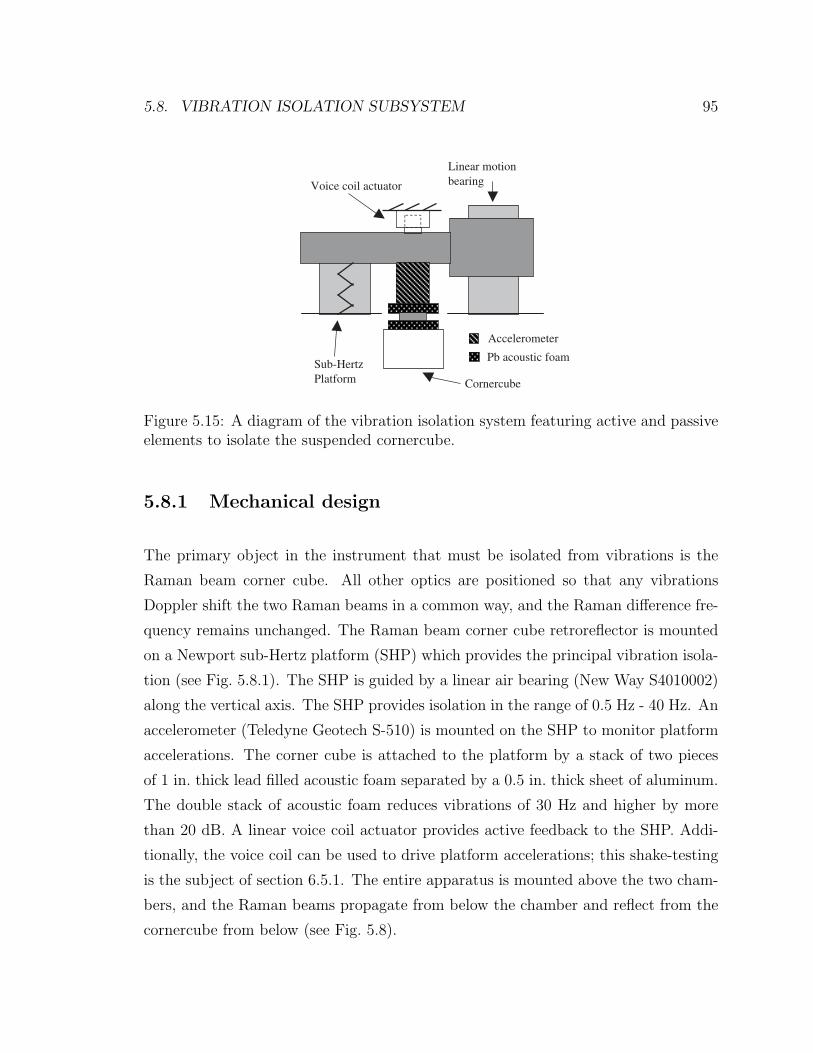
5.8. VIBRATION ISOLATION SUBSYSTEM 95
Voice coil actuator
Sub-HertzPlatform Cornercube
Accelerometer
Pb acoustic foam
Linear motionbearing
Figure 5.15: A diagram of the vibration isolation system featuring active and passiveelements to isolate the suspended cornercube.
5.8.1 Mechanical design
The primary object in the instrument that must be isolated from vibrations is the
Raman beam corner cube. All other optics are positioned so that any vibrations
Doppler shift the two Raman beams in a common way, and the Raman difference fre-
quency remains unchanged. The Raman beam corner cube retroreflector is mounted
on a Newport sub-Hertz platform (SHP) which provides the principal vibration isola-
tion (see Fig. 5.8.1). The SHP is guided by a linear air bearing (New Way S4010002)
along the vertical axis. The SHP provides isolation in the range of 0.5 Hz - 40 Hz. An
accelerometer (Teledyne Geotech S-510) is mounted on the SHP to monitor platform
accelerations. The corner cube is attached to the platform by a stack of two pieces
of 1 in. thick lead filled acoustic foam separated by a 0.5 in. thick sheet of aluminum.
The double stack of acoustic foam reduces vibrations of 30 Hz and higher by more
than 20 dB. A linear voice coil actuator provides active feedback to the SHP. Addi-
tionally, the voice coil can be used to drive platform accelerations; this shake-testing
is the subject of section 6.5.1. The entire apparatus is mounted above the two cham-
bers, and the Raman beams propagate from below the chamber and reflect from the
cornercube from below (see Fig. 5.8).
96 CHAPTER 5. EXPERIMENTAL APPARATUS
5.8.2 DSP servo system
The active servo system for the SHP platform is now described. The active feedback
loop starts with the accelerometer to monitor vibrations. The accelerometer output
is processed by a DSP (Spectrum Signal Indy TMS320C32), which is used to filter
digitally the accelerometer input (as described below) and generate the feedback error
signal. The feedback signal, after being buffered by a voltage amplifier, closes the
feedback loop by driving the voice coil mounted between the SHP and the platform
support. We apply the following digital filters in processing the accelerometer signal.
First, a lag filter with a bandwidth of 1 Hz to 80 Hz rolls off the feedback below the
accelerometer’s 100 Hz high frequency cut-off. Next, a second lag filter with identical
bandwidth is used to make the gain roll-off second order. Finally, two lead filters are
applied to keep the system from oscillating at low frequency near the closed-loop SHP
resonance of 0.03 Hz, which is also close to the internal high pass frequency of the
accelerometer. The two lead filters have bandwidths of 38 mHz - 200 Hz and 380 mHz
- 200 Hz respectively. The total gain of all four filters is 1600. This work is similar
in concept to that reported in Ref. [92]. The transfer functions of the SHP-voice
coil system as well as the filter transfer functions and discrete implementation of the
digital loops are contained in Appendix B.
Using this servo, the vibrations were reduced to near the noise floor of the ac-
celerometer (10−8 g/Hz1/2) over a bandwidth of 40 mHz - 25 Hz. Higher frequencies
are passively attenuated by the acoustic foam. The power spectral density of the
vibrations is plotted in Fig. 5.16. With the addition of the vibration isolation system,
phase noise from accelerations of the corner cube is reduced to less the 1 rad, and least
squares sinusoidal fits may be performed on the fringes for the longest interrogation
times.
5.9 Microwave generation
The generation and delivery of the 9.2 GHz microwave field is briefly described here.
The microwave field is coupled to the atoms through rf horns attached to viewports

5.9. MICROWAVE GENERATION 97
0 Hz 100
10-5g
10-6g
10-7g
10-8g
Acc
eler
atio
n a)
b)c)
Figure 5.16: Power spectral density of the vibrations of the platform, as measured bythe on-board accelerometer. a) Freely floated platform. b) Actively servoed platform.c) Predicted level of vibration for the cornercube mounted on the acoustic foam.
on the MOT chambers. The microwave frequency is tied to a 10 MHz reference,
temperature stabilized, master crystal oscillator (Oscilloquartz OCXO, stability of
1.4× 10⁻¹³ in 1 s). The reference oscillator drives a 100 MHz phase locked oscillator
(PLO, Wenzel 500-0732) which is the input to a Microlambda (MLPE 1162) 9.2 GHz
PLO. The rf is mixed in a single sideband mixer with an ∼ 7.4 MHz signal from an
AWG which is also phase locked to the reference oscillator. The AWG is used to
scan the rf frequency and phase. The mixer output is amplified up to ∼ 1 W and
sent to the horns. The rf power is controlled by the AWG output, and the relative
power to the two chambers can be adjusted with appropriate attenuation in the two
paths. Coupling the microwaves into the chambers by simply directing the horns
towards the MOTs is not an optimal approach. The microwave field is complex in
the chamber due to reflections from the chamber. Across the cloud of atoms, there
is often a significant phase and amplitude variation in the microwave field. However,
the solution to this, construction of an optimized cavity, is hardly optimal either, as
it would restrict optical access to the atoms.
A microwave π/2 - π/2 clock experiment [8] is performed as a diagnostic to check
the phase noise performance of our oscillators and the noise performance of our detec-
tion system. Detection of microwave clock fringes with 1000:1 SNR was shown using
98 CHAPTER 5. EXPERIMENTAL APPARATUS
the normalized detection as described in section 5.7.3 [91]. This SNR is at the atom
shot noise limit for the fountain with no velocity selection (∼ 106 atoms/shot).
Chapter 6
Results
This chapter first details the initials results of the gradiometer, a measurement of the
Earth’s gravity gradient, in section 6.1. Following the implementation of the atomic
fountain and the sensitive detection scheme described in section 5.7, new levels of
sensitivity were achieved [93]. With this enhanced sensitivity, considerable effort
was devoted to the problem of extracting phase information from the two coupled
interference fringes, particularly in the presence of large amounts of common-mode,
vibration-induced phase noise. A thorough discussion of the data analysis routines
employed is given in section 6.2. Using these data extraction methods an analysis of
the sensitivity and accuracy is performed in section 6.3 and 6.4 respectively. Finally,
section 6.5 details studies of the gradiometer in the presence of a noisy reference
platform.
6.1 Proof-of-principle results
The initial measurement performed was a measurement of the Earth’s gravitational
gradient over a 1.1 m baseline [19]. In order to verify that the phase difference
between interference fringes was indeed due to a gravity gradient, the change in the
Earth’s field between the two accelerometers was measured. In this initial experiment,
the MOTs were constructed out of three pairs of retroreflected beams. With this
configuration launching the atoms was not possible, so the total interaction time was
99
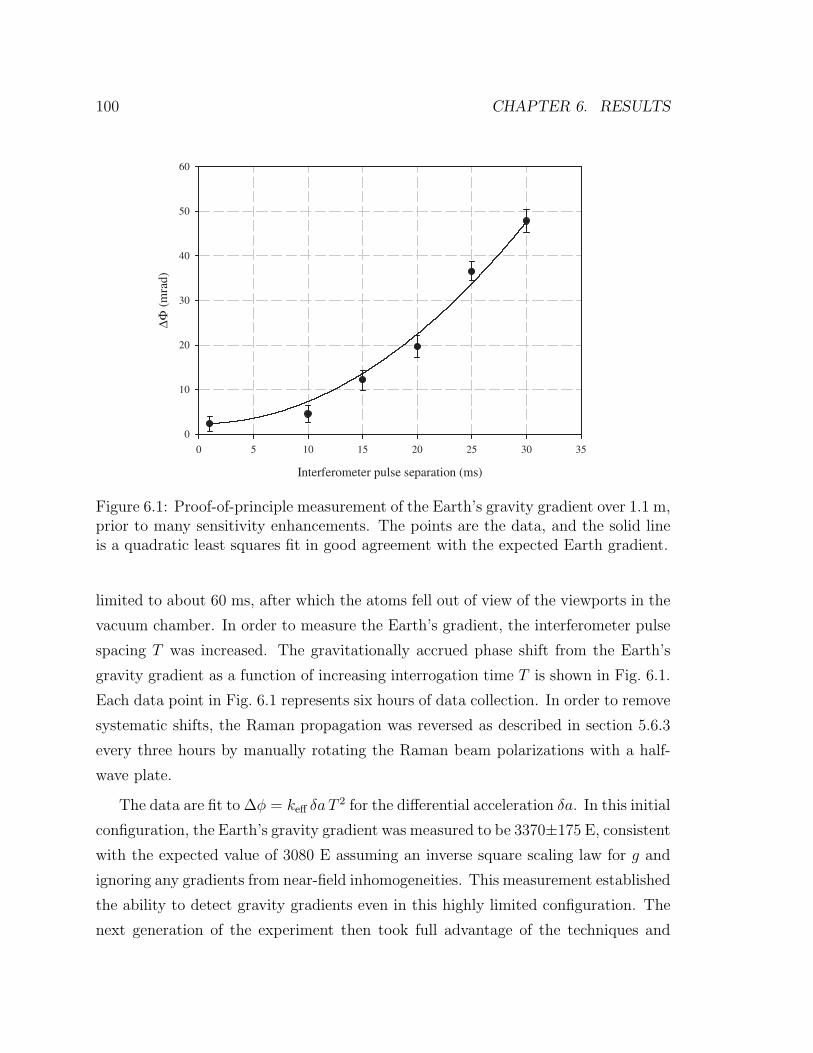
100 CHAPTER 6. RESULTS
Interferometer pulse separation (ms)
0 5 10 15 20 25 30 35
∆Φ (m
rad)
0
10
20
30
40
50
60
Figure 6.1: Proof-of-principle measurement of the Earth’s gravity gradient over 1.1 m,prior to many sensitivity enhancements. The points are the data, and the solid lineis a quadratic least squares fit in good agreement with the expected Earth gradient.
limited to about 60 ms, after which the atoms fell out of view of the viewports in the
vacuum chamber. In order to measure the Earth’s gradient, the interferometer pulse
spacing T was increased. The gravitationally accrued phase shift from the Earth’s
gravity gradient as a function of increasing interrogation time T is shown in Fig. 6.1.
Each data point in Fig. 6.1 represents six hours of data collection. In order to remove
systematic shifts, the Raman propagation was reversed as described in section 5.6.3
every three hours by manually rotating the Raman beam polarizations with a half-
wave plate.
The data are fit to ∆φ = keff δa T2 for the differential acceleration δa. In this initial
configuration, the Earth’s gravity gradient was measured to be 3370±175 E, consistent
with the expected value of 3080 E assuming an inverse square scaling law for g and
ignoring any gradients from near-field inhomogeneities. This measurement established
the ability to detect gravity gradients even in this highly limited configuration. The
next generation of the experiment then took full advantage of the techniques and
6.2. SIGNAL EXTRACTION 101
experimental apparatus described in Chapter 5 to vastly improve the sensitivity and
stability [93].
6.2 Signal extraction
Equally important to the experimental apparatus and the data collection itself is the
signal extraction technique. For this reason different methods of extracting phase
information from the interference fringes were investigated. In order to appreciate
the virtues of the best method, which is based on fitting ellipses to the data, all
methods investigated are described here. The simplest of these methods is nonlinear
least squares sine fitting. This method is the least applicable to noisy data however.
A Gaussian elimination routine is a simple method for dealing with data with high
phase noise, but it can give misleading results if care is not taken and is only suitable
within a small phase range. Fitting the data using a circle fitting method offers
the substantial benefit that it is utterly immune to common-mode phase noise, but
the circle method gives a systematic shift for large relative phase shifts. The most
robust fitting method is a method based on fitting ellipses to the data to extract
the gradiometer phase, and this is the only fitting method that performs well with
nearly all interferometric phases. The methodology is described in this section, and
the experimental figures are given in section 6.3.
6.2.1 Normalization
Before describing the phase extraction methods, the normalization procedure used in
all methods is detailed here. The loading of a vapor cell MOT is a stochastic process,
and even a MOT constructed from highly stable laser beams and magnetic fields will
have number fluctuations. In order to eliminate noise from this fluctuating number
of atoms contributing to the interferometer from shot-to-shot, a normalization is
performed for each interferometer signal based on the two-pulse detection sequence
described in section 5.7. The goal of the normalization is primarily to remove atom
number fluctuations, but also to remove any residual noise from the detection process
102 CHAPTER 6. RESULTS
itself (such as from laser frequency and intensity drifts). After each interferometer
cycle (which represents one gradient measurement) two samples are acquired in each
accelerometer: signals proportional to the F = 4 population and to the differential
population, i.e. proportional to the number of atoms in F = 4 minus the number of
atoms in F = 3. The two samples are combined to infer the total number of atoms
present in the interferometer during each experimental cycle. Let S(1)1 and S
(2)1 be the
signals from the two detection pulses in the first chamber1. S(1)1 is proportional to the
number of atoms in the F = 4 state, and S(2)1 is proportional to the number of atoms
in the F = 4 state minus the number in the F = 3 state, with constants modifying
each state due to small inefficiencies in the detection. The quantity N α S(1)1 − cS
(2)1
then is proportional to the total number of atoms detected in both states, where c
is a constant containing the detection inefficiencies. Dividing the F = 4 interference
fringe produces a normalized signal that is proportional to the transition probability
only:
S1 =S(1)1
Nα
S(1)1
S(1)1 − cS
(2)1
. (6.1)
Performing this normalization removes number fluctuations from the F = 4 interfer-
ence fringe2.
6.2.2 Interference fringe fitting
As described in section 5.6.5, the phase of the final interferometer pulse is scanned
electronically. The most straightforward method of extracting gravity gradient infor-
mation is to determine the gravitationally induced phase shifts in each atom ensemble
by performing least squares sinusoidal fits on the observed interference fringes for each
chamber. This fitting is possible when vibration-induced phase noise is approximately
less than 1 rad. The gravity gradient is obtained by subtracting the two phase shifts
1The same normalization procedure is applied to the second chamber, but with slightly adjustedproportionality constants.
2It is important to note that shot-to-shot number fluctuations are not equivalent to shot noise.Shot noise arises from the statistics of projecting the superposition state of the interferometer ontothe two basis states during the detection. Shot-to-shot number fluctuations primarily come fromnoise on the trapping lasers.
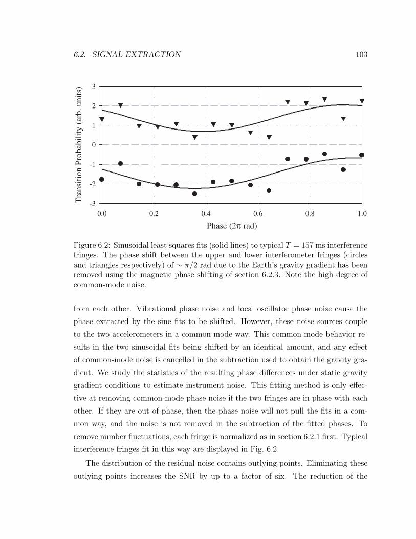
6.2. SIGNAL EXTRACTION 103
Phase (2π rad)
0.0 0.2 0.4 0.6 0.8 1.0
Tra
nsit
ion
Prob
abil
ity
(arb
. uni
ts)
-3
-2
-1
0
1
2
3
Figure 6.2: Sinusoidal least squares fits (solid lines) to typical T = 157 ms interferencefringes. The phase shift between the upper and lower interferometer fringes (circlesand triangles respectively) of ∼ π/2 rad due to the Earth’s gravity gradient has beenremoved using the magnetic phase shifting of section 6.2.3. Note the high degree ofcommon-mode noise.
from each other. Vibrational phase noise and local oscillator phase noise cause the
phase extracted by the sine fits to be shifted. However, these noise sources couple
to the two accelerometers in a common-mode way. This common-mode behavior re-
sults in the two sinusoidal fits being shifted by an identical amount, and any effect
of common-mode noise is cancelled in the subtraction used to obtain the gravity gra-
dient. We study the statistics of the resulting phase differences under static gravity
gradient conditions to estimate instrument noise. This fitting method is only effec-
tive at removing common-mode phase noise if the two fringes are in phase with each
other. If they are out of phase, then the phase noise will not pull the fits in a com-
mon way, and the noise is not removed in the subtraction of the fitted phases. To
remove number fluctuations, each fringe is normalized as in section 6.2.1 first. Typical
interference fringes fit in this way are displayed in Fig. 6.2.
The distribution of the residual noise contains outlying points. Eliminating these
outlying points increases the SNR by up to a factor of six. The reduction of the
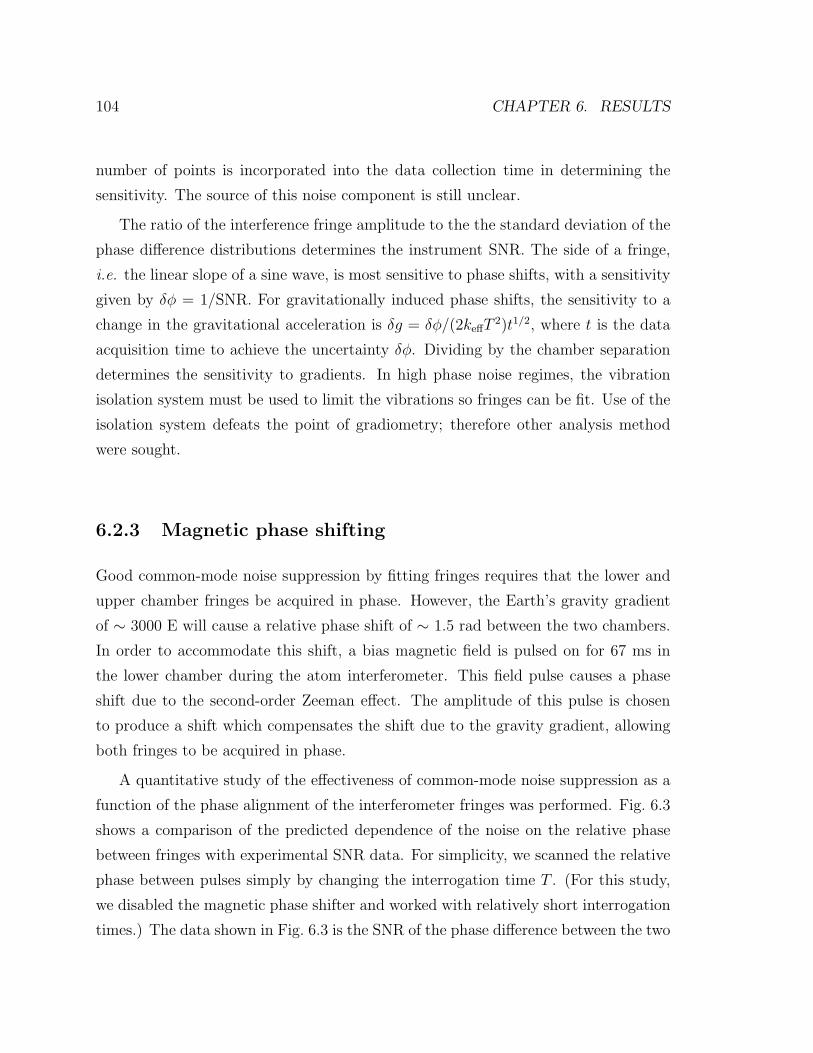
104 CHAPTER 6. RESULTS
number of points is incorporated into the data collection time in determining the
sensitivity. The source of this noise component is still unclear.
The ratio of the interference fringe amplitude to the the standard deviation of the
phase difference distributions determines the instrument SNR. The side of a fringe,
i.e. the linear slope of a sine wave, is most sensitive to phase shifts, with a sensitivity
given by δφ = 1/SNR. For gravitationally induced phase shifts, the sensitivity to a
change in the gravitational acceleration is δg = δφ/(2keffT2)t1/2, where t is the data
acquisition time to achieve the uncertainty δφ. Dividing by the chamber separation
determines the sensitivity to gradients. In high phase noise regimes, the vibration
isolation system must be used to limit the vibrations so fringes can be fit. Use of the
isolation system defeats the point of gradiometry; therefore other analysis method
were sought.
6.2.3 Magnetic phase shifting
Good common-mode noise suppression by fitting fringes requires that the lower and
upper chamber fringes be acquired in phase. However, the Earth’s gravity gradient
of ∼ 3000 E will cause a relative phase shift of ∼ 1.5 rad between the two chambers.
In order to accommodate this shift, a bias magnetic field is pulsed on for 67 ms in
the lower chamber during the atom interferometer. This field pulse causes a phase
shift due to the second-order Zeeman effect. The amplitude of this pulse is chosen
to produce a shift which compensates the shift due to the gravity gradient, allowing
both fringes to be acquired in phase.
A quantitative study of the effectiveness of common-mode noise suppression as a
function of the phase alignment of the interferometer fringes was performed. Fig. 6.3
shows a comparison of the predicted dependence of the noise on the relative phase
between fringes with experimental SNR data. For simplicity, we scanned the relative
phase between pulses simply by changing the interrogation time T . (For this study,
we disabled the magnetic phase shifter and worked with relatively short interrogation
times.) The data shown in Fig. 6.3 is the SNR of the phase difference between the two
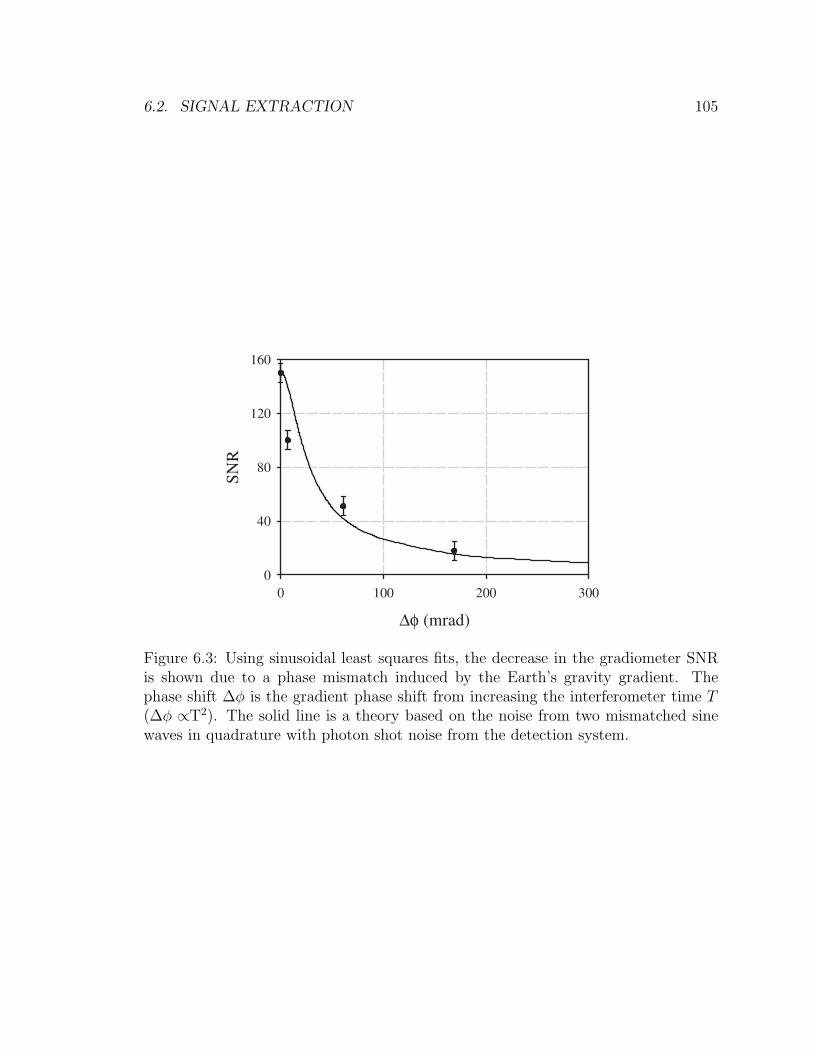
6.2. SIGNAL EXTRACTION 105
∆φ (mrad)
0 100 200 300
SNR
0
40
80
120
160
Figure 6.3: Using sinusoidal least squares fits, the decrease in the gradiometer SNRis shown due to a phase mismatch induced by the Earth’s gravity gradient. Thephase shift ∆φ is the gradient phase shift from increasing the interferometer time T(∆φ ∝T2). The solid line is a theory based on the noise from two mismatched sinewaves in quadrature with photon shot noise from the detection system.

106 CHAPTER 6. RESULTS
fringes obtained by performing least squares fits as described above on a set of inter-
ference fringes. The prediction is the simulated SNR of the phase difference between
two phase-mismatched sine functions with phase noise added. The predicted SNR
is added in quadrature with uncorrelated detection noise noise in order to compare
the simulation with experimental data in this curve. As shown, the data is in good
agreement with the theory, demonstrating the need for the magnetic phase shifting
pulse with this analysis routine.
One concern is that by adding an extra bias field, absolute accuracy and long-term
stability will be sacrificed. To study this, the stability of the bias field used in the
magnetic shifter has also been studied. High frequency noise on this bias field could
lead to extra phase noise on the gravity gradient signals as well. This noise has been
investigated by applying a bias pulse in a microwave clock π/2-π/2 experiment and
comparing the SNR for a weak pulse (phase shift ∼ 1.2 rad) and a strong field pulse
(phase shift ∼ 67 rad). For the large phase shift, no extra phase noise or drift is seen
at a fractional uncertainty in the phase of less than 3× 10⁻⁶. This implies that for a
1 rad shift, the bias pulse contributes noise at a level below 8 × 10⁻¹³g. However, it
is certain that at some level below this, the stability level is not sufficient for making
ultra-precise measurements. For such measurements, adding possible systematics like
a magnetic field is undesirable.
6.2.4 Gaussian elimination reduction
In the case where phase noise is greater than 1 rad, the noise renders it impossible
to characterize instrument noise using the least squares method described above.
In the most sensitive modes of operation, the vibrations of the reference platform
induced phase noise much larger than this level. A different analysis technique can
be performed in this regime, using a point-by-point analysis. After collection of
the gradiometer data, the normalization algorithm is applied to remove common
amplitude fluctuations in each chamber. After removing amplitude noise, a cross-
chamber normalization is performed to reject phase noise that is primarily vibration-
induced.
6.2. SIGNAL EXTRACTION 107
The details of this noise analysis procedure are as follows. The two interferometer
fringes are first normalized using the procedure of section 6.2.1. To remove common
phase noise between the two chambers, a series of experimental cycles is taken (typ-
ically 16), and a least squares minimization (via Gaussian elimination) is performed
on the quantity (S1 − αS2 − β)2 where S1 and S2 are the shot-by-shot normalized
F = 4 population levels from the two interferometers. The fit constants α and β
are used to compensate for possible differences in interference contrast between the
two accelerometers. The rationale behind this analysis method is that in the limit of
small relative phase shift ∆φ, the difference between the two fringes is:
sin(φ) − sin(φ + ∆φ) ∆φ cos(φ). (6.2)
Even more appealing, at the zero crossing of the sine waves when φ = 0 or π, this
difference reduces to just ∆φ. Thus with this method, the phase shift is directly
proportional to the offset β used to perform the Gaussian elimination. This method
is ideally employed not by scanning fringes, but by acquiring data only on the side of
a fringe (which is difficult to do in a high phase noise environment).
The residuals of the Gaussian elimination procedure are used to estimate instru-
ment noise, as show in Fig. 6.4. Again, this distribution is non-Gaussian, and outlying
points are discarded to obtain SNR and short-term sensitivity estimates. However,
the Gaussian elimination routine is an unsatisfying data reduction method. If the
relative efficiencies of the detection pulses changes, it is possible to be misled by the
data analysis. Because of the nature of the signal acquisition and the subtraction, if
care is not taken with the analysis, it is possible to obtain artificially small residuals,
producing an erroneously high SNR. Finally it requires the addition of a bias field
(as described in section 6.2.3) to operate at a nearly perfectly in-phase condition to
obtain good common-mode suppression between the two chambers.

108 CHAPTER 6. RESULTS
Phase (2π rad)
0.0 0.2 0.4 0.6 0.8 1.0
Sig
nal (
arb.
uni
ts)
-0.2
-0.1
0.0
0.1
0.2
Figure 6.4: Gradiometer interference fringes with T = 157.5 ms. Squares and circlesrepresent the normalized upper and lower chamber fringes respectively, after compen-sating for contrast differences between the chambers. Triangles show the lower cham-ber residual signals after reducing the data using the Gaussian elimination methodsection 6.2.4.
6.2.5 Circle fitting
An innovative method for extracting the phase from the gradiometer relies on the
trigonometric relationship between two coupled sinusoids3. If the data S1 and S2 are
two sinusoids, sin(θ) and cos(θ + ∆φ), out of phase by approximately π/2 rad, i.e.
∆φ is small, then the data lies approximately on a circle of radius r when plotted
as the interference fringe for one accelerometer versus the other. The virtue of this
method is that it is totally immune to common-mode phase noise; the data points
always lie on the circle, no matter what the phase noise is, as long as it is common
to both interferometers. The radius of the circle is defined as:
r2 ≡ S21 + S2
2 = sin2(θ) + cos2(θ + ∆φ) 1. (6.3)
3This method is applicable for any system of coupled sinusoids with an appropriate phase rela-tionship of ∼ π/2 rad.
6.2. SIGNAL EXTRACTION 109
Simplifying and rearranging this equation leads to:
r2 − 1 = sin(4θ + 2∆φ) sin(∆φ). (6.4)
Experimentally, the angle θ is extracted for each point using the relationship:
θ′ = tan−1(S2
S1
), (6.5)
where θ′ = 2θ due to the range of tan−1. It is then straightforward to extract the
phase from equation 6.4, by either performing a least squares fit to the function
∆φ = sin−1
(r2 − 1
sin(2θ′)
)(6.6)
or by using a computationally faster Fourier analysis4 by multiplying both sides of
equation 6.4 by sin(2θ′) and summing over all θ′:
∆φ =
∑θ′
(r2 − 1)sin(2θ′)∑θ′
sin2(2θ′). (6.7)
The key approximation in this approach is sin(4θ + 2∆φ) sin(4θ), which is only
true in the limit of small ∆φ.
To summarize, in the limit of two sinusoids out of phase by nearly π/2 rad, the
data lies close to a circle when plotted as one sinusoid versus the other. The deviations
from a perfect circle are due to slight phase deviations from π/2 and are sensitive
to small phase shifts. Fitting these deviations allows for extraction of the phase
difference between the chambers. Before fitting, the data is normalized using the
two detection pulses as described in section 6.2.1. Then a circle is fit to the data to
normalize it to the unit circle; this fit is performed merely to adjust the scaling and
offset parameters for each fringe. For the typical parameters in this experiment the
gravity gradient of the Earth conveniently causes a shift of ∼ π/2 rad between the two
4The Fourier approach only works in the limit of a large number of points that sample uniformlyover the circle.
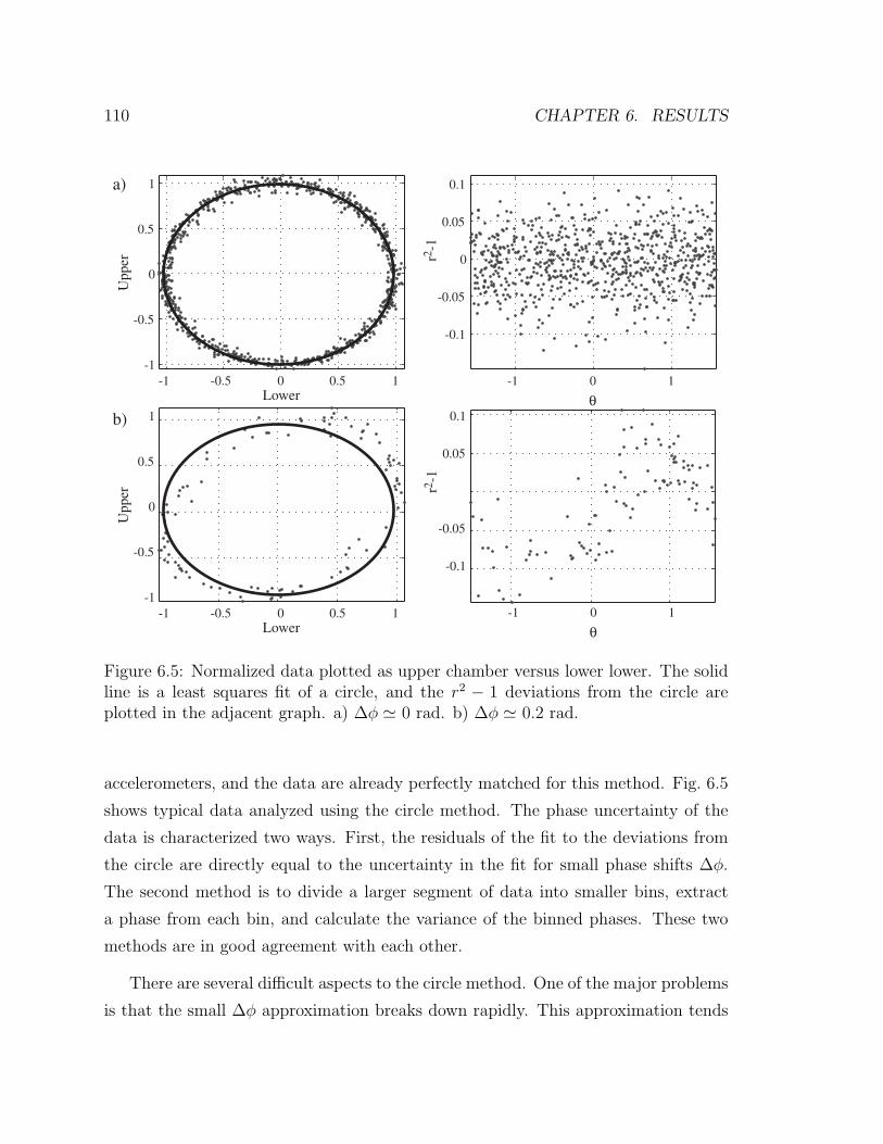
110 CHAPTER 6. RESULTS
0
-1 0 1
-0.1
-0.05
0.05
0.1
r2-1
θ-1 -0.5 0 0.5 1
-1
-0.5
0
0.5
1
Lower
Upp
er
-1 -0.5 0 0.5 1-1
-0.5
0
0.5
1
Lower
Upp
er
-1 0 1
-0.1
-0.05
0.05
0.1r2
-1
θ
a)
b)
Figure 6.5: Normalized data plotted as upper chamber versus lower lower. The solidline is a least squares fit of a circle, and the r2 − 1 deviations from the circle areplotted in the adjacent graph. a) ∆φ 0 rad. b) ∆φ 0.2 rad.
accelerometers, and the data are already perfectly matched for this method. Fig. 6.5
shows typical data analyzed using the circle method. The phase uncertainty of the
data is characterized two ways. First, the residuals of the fit to the deviations from
the circle are directly equal to the uncertainty in the fit for small phase shifts ∆φ.
The second method is to divide a larger segment of data into smaller bins, extract
a phase from each bin, and calculate the variance of the binned phases. These two
methods are in good agreement with each other.
There are several difficult aspects to the circle method. One of the major problems
is that the small ∆φ approximation breaks down rapidly. This approximation tends
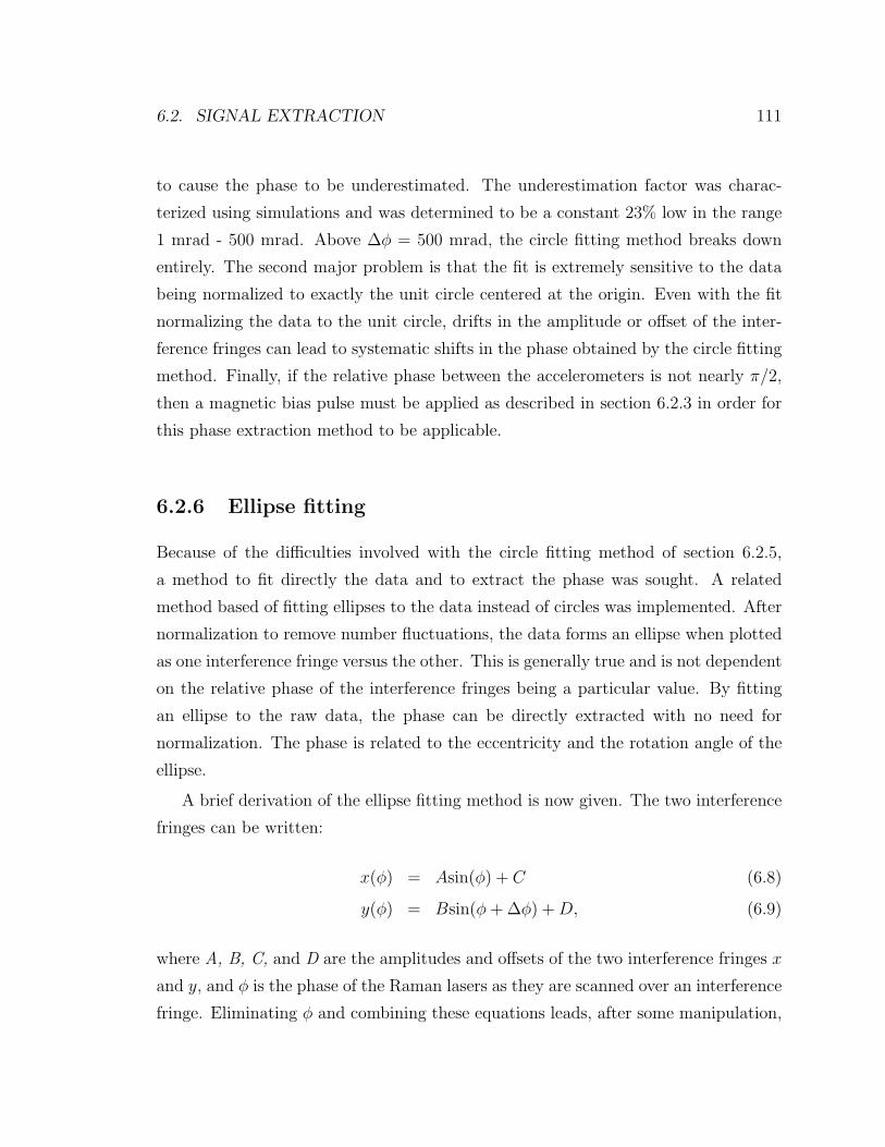
6.2. SIGNAL EXTRACTION 111
to cause the phase to be underestimated. The underestimation factor was charac-
terized using simulations and was determined to be a constant 23% low in the range
1 mrad - 500 mrad. Above ∆φ = 500 mrad, the circle fitting method breaks down
entirely. The second major problem is that the fit is extremely sensitive to the data
being normalized to exactly the unit circle centered at the origin. Even with the fit
normalizing the data to the unit circle, drifts in the amplitude or offset of the inter-
ference fringes can lead to systematic shifts in the phase obtained by the circle fitting
method. Finally, if the relative phase between the accelerometers is not nearly π/2,
then a magnetic bias pulse must be applied as described in section 6.2.3 in order for
this phase extraction method to be applicable.
6.2.6 Ellipse fitting
Because of the difficulties involved with the circle fitting method of section 6.2.5,
a method to fit directly the data and to extract the phase was sought. A related
method based of fitting ellipses to the data instead of circles was implemented. After
normalization to remove number fluctuations, the data forms an ellipse when plotted
as one interference fringe versus the other. This is generally true and is not dependent
on the relative phase of the interference fringes being a particular value. By fitting
an ellipse to the raw data, the phase can be directly extracted with no need for
normalization. The phase is related to the eccentricity and the rotation angle of the
ellipse.
A brief derivation of the ellipse fitting method is now given. The two interference
fringes can be written:
x(φ) = Asin(φ) + C (6.8)
y(φ) = Bsin(φ + ∆φ) + D, (6.9)
where A, B, C, and D are the amplitudes and offsets of the two interference fringes x
and y, and φ is the phase of the Raman lasers as they are scanned over an interference
fringe. Eliminating φ and combining these equations leads, after some manipulation,
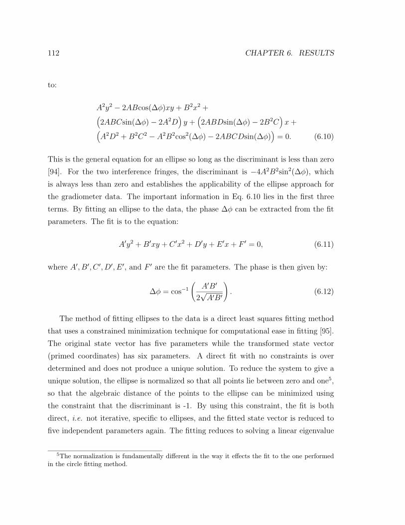
112 CHAPTER 6. RESULTS
to:
A2y2 − 2ABcos(∆φ)xy + B2x2 +(2ABCsin(∆φ) − 2A2D
)y +
(2ABDsin(∆φ) − 2B2C
)x +(
A2D2 + B2C2 − A2B2cos2(∆φ) − 2ABCDsin(∆φ))
= 0. (6.10)
This is the general equation for an ellipse so long as the discriminant is less than zero
[94]. For the two interference fringes, the discriminant is −4A2B2sin2(∆φ), which
is always less than zero and establishes the applicability of the ellipse approach for
the gradiometer data. The important information in Eq. 6.10 lies in the first three
terms. By fitting an ellipse to the data, the phase ∆φ can be extracted from the fit
parameters. The fit is to the equation:
A′y2 + B′xy + C ′x2 + D′y + E ′x + F ′ = 0, (6.11)
where A′, B′, C ′, D′, E ′, and F ′ are the fit parameters. The phase is then given by:
∆φ = cos−1
(A′B′
2√A′B′
). (6.12)
The method of fitting ellipses to the data is a direct least squares fitting method
that uses a constrained minimization technique for computational ease in fitting [95].
The original state vector has five parameters while the transformed state vector
(primed coordinates) has six parameters. A direct fit with no constraints is over
determined and does not produce a unique solution. To reduce the system to give a
unique solution, the ellipse is normalized so that all points lie between zero and one5,
so that the algebraic distance of the points to the ellipse can be minimized using
the constraint that the discriminant is -1. By using this constraint, the fit is both
direct, i.e. not iterative, specific to ellipses, and the fitted state vector is reduced to
five independent parameters again. The fitting reduces to solving a linear eigenvalue
5The normalization is fundamentally different in the way it effects the fit to the one performedin the circle fitting method.
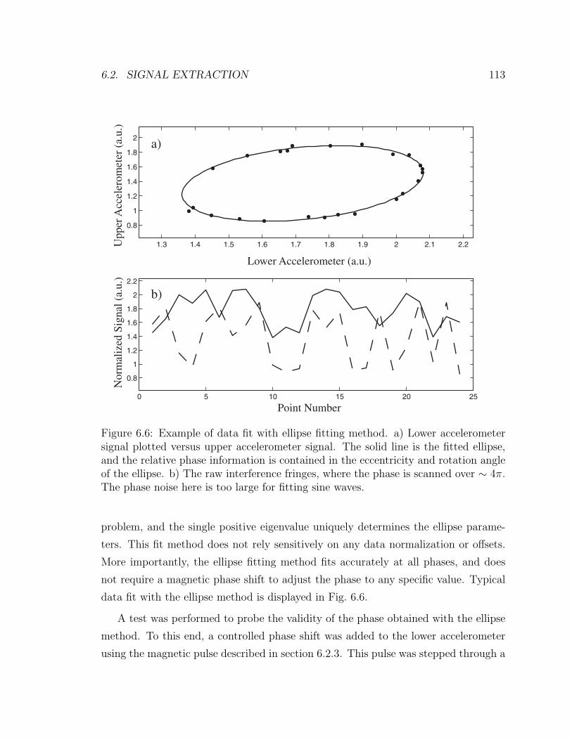
6.2. SIGNAL EXTRACTION 113
1.3 1.4 1.5 1.6 1.7 1.8 1.9 2 2.1 2.2
0.8
1
1.2
1.4
1.6
1.8
2
0 5 10 15 20 25
0.8
1
1.2
1.4
1.6
1.8
2
2.2
Lower Accelerometer (a.u.)
Upp
er A
ccel
erom
eter
(a.
u.)
Point Number
Nor
mal
ized
Sig
nal (
a.u.
)
a)
b)
Figure 6.6: Example of data fit with ellipse fitting method. a) Lower accelerometersignal plotted versus upper accelerometer signal. The solid line is the fitted ellipse,and the relative phase information is contained in the eccentricity and rotation angleof the ellipse. b) The raw interference fringes, where the phase is scanned over ∼ 4π.The phase noise here is too large for fitting sine waves.
problem, and the single positive eigenvalue uniquely determines the ellipse parame-
ters. This fit method does not rely sensitively on any data normalization or offsets.
More importantly, the ellipse fitting method fits accurately at all phases, and does
not require a magnetic phase shift to adjust the phase to any specific value. Typical
data fit with the ellipse method is displayed in Fig. 6.6.
A test was performed to probe the validity of the phase obtained with the ellipse
method. To this end, a controlled phase shift was added to the lower accelerometer
using the magnetic pulse described in section 6.2.3. This pulse was stepped through a

114 CHAPTER 6. RESULTS
Applied magnetic phase shift (rad)0 2 4 6 8
Fitte
d ph
ase
shif
t (ra
d)
0.0
0.5
1.0
1.5
2.0
2.5
3.0
Figure 6.7: Relative phase extracted from T = 150 ms interference fringes using theellipse fitting routine. The relative phase was varied with a magnetic field pulse.
range of phases and the phase extracted from the ellipse method was compared with
the expected phase. The expected phase shift was calibrated by measuring the shift
produced by an applied magnetic phase shift (measured using an identical magnetic
field pulse in a microwave π/2−π/2 clock experiment) and fitting the resultant phase
shift using the ellipse method. The results of this calibration are shown in Fig. 6.7.
The ellipse fitted phases are a linear function of the expected phases (modulo π and
an overall sign due to the cos−1 in equation 6.12) except for interesting features near
the phases 0 and π rad. It appears as if the phase “rolls off” near these values. It
is easy to understand why this is. Near 0 and π rad, the two fringes are in phase or
completely out of phase, and the ellipse becomes so eccentric it is essentially a line6.
With a small amount of amplitude noise, the ellipse will never actually become a line,
and the ellipse fit will never produce a phase extremely close to these phases for data
with noise. In this limited situation, the ellipse fitting method is not appropriate,
or a bias magnetic field must be applied to shift away from this area. However over
the bulk of the range of phases, the ellipse method performs accurately. One other
disadvantage of the ellipse fitting method is that it is sensitive to extreme outliers
6At exactly these phase values, with no noise, there is a singularity in the fitting routine, butthis is a technical detail and not experimentally observable.
6.2. SIGNAL EXTRACTION 115
outside of the ellipse; these points will strongly pull the fit. However, it is not difficult
to reject these wild points.
The phase uncertainty of the phase extracted with this method is calculated using
a distance metric. After the eigenvalue problem is solved to obtain the fit constants
for equation 6.10, then the data is inserted into the left-hand side of the equation
using the fit constants. This value is a distance metric from the fitted ellipse, and
the phase uncertainty of the ellipse is related to the square root of the average of the
distance metrics over all point in the fit. It is not obvious how the distance metric
is specifically related to the phase uncertainty of the fit. To study this, simulations
were performed using simulated interference fringes with common phase noise and
non-common amplitude noise of up to 10%, which is even larger than the residual
noise of the actual data. It was found that the distance metric overestimates the noise
by ∼ 50%, but fits the phase accurately unless the non-common noise is extremely
large. Again, to verify this analysis, a large section of data was binned into smaller
bins and the variance of the phase extracted from each bin was calculated. These two
methods agree well with each other.
6.2.7 Summary of data extraction methods
Under the appropriate circumstances, all four data extraction methods are capable
of extracting the correct phase shifts. When each extraction technique is employed
in its optimal operating environment, all give similar SNRs and long-term drift per-
formance. However, due to the misleading results obtained using the circle fitting
method and Gaussian elimination, they are no longer employed. The method of fit-
ting fringes is always unambiguous, but it is not always effective at removing common
phase noise, nor is it even able to fit properly in high phase noise situations. The
ellipse fitting method is the method of choice in terms of both accuracy and computa-
tional speed. It is the only fitting method that can extract phases at nearly all relative
phases and is not sensitive to common-mode phase noise at any position. For these
reasons it is the predominant fitting method currently employed in the gradiometer.
As this method was pioneered towards the end of the work presented herein, much
116 CHAPTER 6. RESULTS
of the data analysis was performed using the fringe fitting and Gaussian elimination
methods.
6.3 Sensitivity characterization
Each interference fringe is typically recorded with sixteen consecutive cycles of the
experiment. The number of points per scan is kept small to decrease sensitivity to
long term drifts in signal amplitude and contrast. The source of such drifts include
fluctuations in laser power and drifts in the Cs vapor pressure in the vacuum chambers.
The normalized data reduction methods described in section 6.2 are performed on
the data. The three high phase noise methods of data extraction all agree well
with each other, particularly for short-term sensitivity. The resulting observed SNR
is typically 150:1. This corresponds to a differential accelerometer performance of
4 × 10⁻⁸ m/s2/Hz1/2, or ∼ 4 × 10⁻⁹ g/Hz1/2. Scaling this to a 10 m baseline gives
an inferred gradient sensitivity of 4 E/Hz1/2. Figs. 6.4, 6.5, and 6.6 all show typical
high sensitivity fringes in the upper and lower chamber for a T = 150 ms - 157.5 ms
interferometer. The fringe contrast is typically ∼ 33%.
Fig. 6.8 compares interference phase scans with the reference platform rigidly
attached to the optical table (∼ 10−5g acceleration noise) with the reference platform
servoed using the vibration isolation system. We can use the data acquired under
servoed conditions (e.g. Fig. 6.8b) to provide an independent check on the observed
SNR, by performing the least-squares fitting analysis detailed in section 6.2.2, and
comparing it with the high phase noise analysis methods for data acquired without
the servo (e.g. Fig. 6.8a). We find that all approaches yield consistent noise estimates
when operated optimally. However, as noted above, when the fitting methods are not
in their optimal conditions, then inaccuracies can result. The ellipse fitting method
is the most suitable method, based on its accuracy, simplicity, and computational
speed, for data which does not have egregious outliers, as is the case with the typical
gradiometer data.
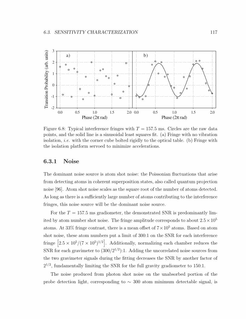
6.3. SENSITIVITY CHARACTERIZATION 117
Phase (2π rad)0.0 0.5 1.0 1.5 2.0
Phase (2π rad)0.0 0.5 1.0 1.5 2.0
Tran
sitio
n Pr
obab
ility
(arb
. uni
ts)
-2
-1
0
1
2
3a) b)
Figure 6.8: Typical interference fringes with T = 157.5 ms. Circles are the raw datapoints, and the solid line is a sinusoidal least squares fit. (a) Fringe with no vibrationisolation, i.e. with the corner cube bolted rigidly to the optical table. (b) Fringe withthe isolation platform servoed to minimize accelerations.
6.3.1 Noise
The dominant noise source is atom shot noise: the Poissonian fluctuations that arise
from detecting atoms in coherent superposition states, also called quantum projection
noise [96]. Atom shot noise scales as the square root of the number of atoms detected.
As long as there is a sufficiently large number of atoms contributing to the interference
fringes, this noise source will be the dominant noise source.
For the T = 157.5 ms gradiometer, the demonstrated SNR is predominantly lim-
ited by atom number shot noise. The fringe amplitude corresponds to about 2.5×10⁵
atoms. At 33% fringe contrast, there is a mean offset of 7×10⁵ atoms. Based on atom
shot noise, these atom numbers put a limit of 300:1 on the SNR for each interference
fringe[2.5 × 10⁵/(7 × 105)1/2
]. Additionally, normalizing each chamber reduces the
SNR for each gravimeter to (300/21/2):1. Adding the uncorrelated noise sources from
the two gravimeter signals during the fitting decreases the SNR by another factor of
21/2, fundamentally limiting the SNR for the full gravity gradiometer to 150:1.
The noise produced from photon shot noise on the unabsorbed portion of the
probe detection light, corresponding to ∼ 300 atom minimum detectable signal, is
118 CHAPTER 6. RESULTS
approximately at the 800:1 level for each individual fringe, giving about a 400:1 limit
after the normalization and differential phase extraction of the two fringes. This
means that photon shot noise does not impose a substantial SNR limit for the current
number of atoms, but it would become significant for reduced atom numbers.
6.3.2 Proof-of-principle mass detection
In order to demonstrate further the sensitivity of the gravity gradiometer, measure-
ment of the gradient of a nearby object was performed. With the sensitivity improved
beyond the proo-of-principle results of section 6.1, a measurement of the gravity gra-
dient from small test masses has been made [93]. For this measurement, eight lead
bricks (∼ 12.5 kg each) were placed symmetrically near the lower accelerometer, ∼0.2 m from the apex of the atomic fountain. The calculated acceleration from this
configuration of mass was 8.2 × 10⁻⁹g. The results of this measurement are shown
in Fig. 6.9. Using the Gaussian elimination method of data reduction, the steps in
the phase as the lead is place near the chamber and then removed again are clear.
The measured acceleration is 8.1 ± 2.1 × 10⁻⁹g which agrees well with the expected
phase shift. Because the mass is a crude mass, the expected phase is only calculated
to about 25%.
6.4 Accuracy estimation
6.4.1 Tidal measurement
To demonstrate accelerometer (hence gradiometer) accuracy, the accelerometer out-
puts were monitored over extended periods of time. As in [97] the daily fluctuations
in the measured acceleration due to gravity induced by the motion of the Sun and
Moon are observed. Fig. 6.10 shows data from one accelerometer taken over a period
of several days compared to the Tamura 87 tide model [98]. The only free parameter
in this fit is an overall phase offset. From this data set, we constrain the accelerometer
phase offset to better than 10−9g over the two day measurement cycle. Subsequent
measurements, taken several weeks later, resulted in a similar determination of the
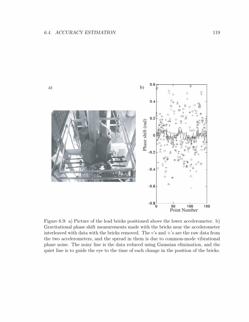
6.4. ACCURACY ESTIMATION 119
a) b)
Point Number
Phas
e sh
ift (
rad)
Figure 6.9: a) Picture of the lead bricks positioned above the lower accelerometer. b)Gravitational phase shift measurements made with the bricks near the accelerometerinterleaved with data with the bricks removed. The ’s and +’s are the raw data fromthe two accelerometers, and the spread in them is due to common-mode vibrationalphase noise. The noisy line is the data reduced using Gaussian elimination, and thequiet line is to guide the eye to the time of each change in the position of the bricks.
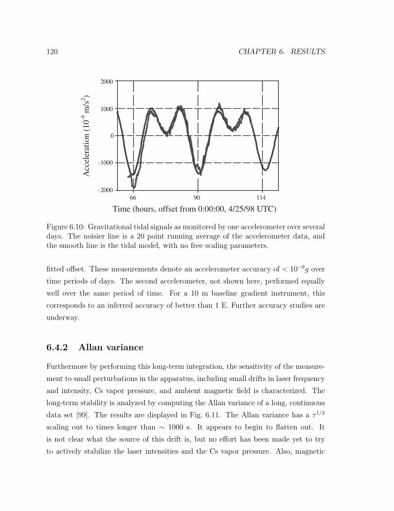
120 CHAPTER 6. RESULTS
Acc
eler
atio
n (1
0-9 m
/s2 )
Time (hours, offset from 0:00:00, 4/25/98 UTC)
-2000
-1000
0
1000
2000
66 90 114
Figure 6.10: Gravitational tidal signals as monitored by one accelerometer over severaldays. The noisier line is a 20 point running average of the accelerometer data, andthe smooth line is the tidal model, with no free scaling parameters.
fitted offset. These measurements denote an accelerometer accuracy of < 10−9g over
time periods of days. The second accelerometer, not shown here, performed equally
well over the same period of time. For a 10 m baseline gradient instrument, this
corresponds to an inferred accuracy of better than 1 E. Further accuracy studies are
underway.
6.4.2 Allan variance
Furthermore by performing this long-term integration, the sensitivity of the measure-
ment to small perturbations in the apparatus, including small drifts in laser frequency
and intensity, Cs vapor pressure, and ambient magnetic field is characterized. The
long-term stability is analyzed by computing the Allan variance of a long, continuous
data set [99]. The results are displayed in Fig. 6.11. The Allan variance has a τ 1/2
scaling out to times longer than ∼ 1000 s. It appears to begin to flatten out. It
is not clear what the source of this drift is, but no effort has been made yet to try
to actively stabilize the laser intensities and the Cs vapor pressure. Also, magnetic
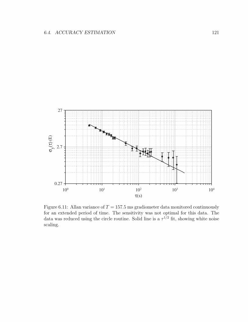
6.4. ACCURACY ESTIMATION 121
τ(s)100 101 102 103 104
σ y(τ)
27
2.7
0.27
(E)
Figure 6.11: Allan variance of T = 157.5 ms gradiometer data monitored continuouslyfor an extended period of time. The sensitivity was not optimal for this data. Thedata was reduced using the circle routine. Solid line is a τ 1/2 fit, showing white noisescaling.

122 CHAPTER 6. RESULTS
Figure 6.12: The precision lead tests masses for the G measurement before beingplaced near the accelerometers and suspended above the lower accelerometer.
shielding might reduce this long-term drift.
6.4.3 Gravitational constant measurement
In order to investigate further the instrument stability as well as to perform one of the
scientifically interesting measurements discussed in section 2.3, a proof-of-principle
measurement of the gravitational constant has been initiated. The concept of this
experiment is to measure the gravitational field of a well-characterized test mass as
it is brought close to one of the accelerometers in the gradiometer. To this goal,
there are two key aspects to the measurement: the precision to which the test mass
is characterized and the stability of the experiment over the time needed to measure
the test mass to the desired precision.
It is not a trivial matter to obtain a test mass with a uniform density and precise
dimensions, particularly one that is suitable for the geometry of the experiment. For
our measurements of G, the tests masses are 20 14 in. diameter open bore ultra-pure
lead cylinders, each 1 in. high (see Fig. 6.12). The open bore is just large enough to
allow the Raman beams to pass through when the lead cylinders are placed above the
lower accelerometer. The lead is specified to be 99.99% pure. Each lead disc weighs
about 50 lbs and can be measured accurately to greater than a part per 104 using a
calibrated scale. The tolerances on the dimensions are all such that the volume of the
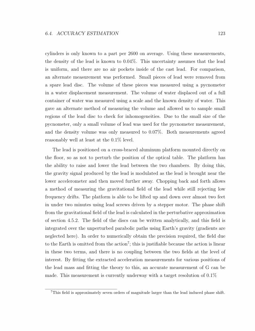
6.4. ACCURACY ESTIMATION 123
cylinders is only known to a part per 2600 on average. Using these measurements,
the density of the lead is known to 0.04%. This uncertainty assumes that the lead
is uniform, and there are no air pockets inside of the cast lead. For comparison,
an alternate measurement was performed. Small pieces of lead were removed from
a spare lead disc. The volume of these pieces was measured using a pycnometer
in a water displacement measurement. The volume of water displaced out of a full
container of water was measured using a scale and the known density of water. This
gave an alternate method of measuring the volume and allowed us to sample small
regions of the lead disc to check for inhomogeneities. Due to the small size of the
pycnometer, only a small volume of lead was used for the pycnometer measurement,
and the density volume was only measured to 0.07%. Both measurements agreed
reasonably well at least at the 0.1% level.
The lead is positioned on a cross-braced aluminum platform mounted directly on
the floor, so as not to perturb the position of the optical table. The platform has
the ability to raise and lower the lead between the two chambers. By doing this,
the gravity signal produced by the lead is modulated as the lead is brought near the
lower accelerometer and then moved further away. Chopping back and forth allows
a method of measuring the gravitational field of the lead while still rejecting low
frequency drifts. The platform is able to be lifted up and down over almost two feet
in under two minutes using lead screws driven by a stepper motor. The phase shift
from the gravitational field of the lead is calculated in the perturbative approximation
of section 4.5.2. The field of the discs can be written analytically, and this field is
integrated over the unperturbed parabolic paths using Earth’s gravity (gradients are
neglected here). In order to numerically obtain the precision required, the field due
to the Earth is omitted from the action7; this is justifiable because the action is linear
in these two terms, and there is no coupling between the two fields at the level of
interest. By fitting the extracted acceleration measurements for various positions of
the lead mass and fitting the theory to this, an accurate measurement of G can be
made. This measurement is currently underway with a target resolution of 0.1%
7This field is approximately seven orders of magnitude larger than the lead induced phase shift.
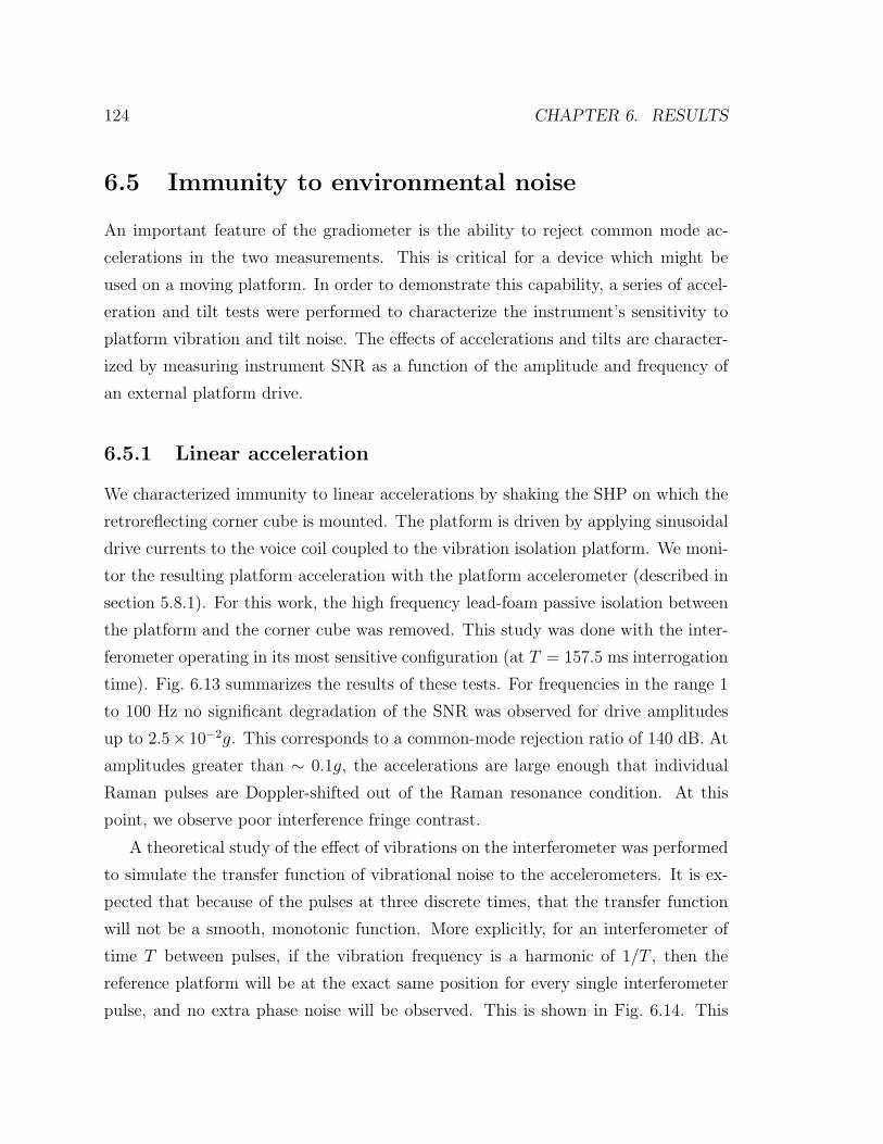
124 CHAPTER 6. RESULTS
6.5 Immunity to environmental noise
An important feature of the gradiometer is the ability to reject common mode ac-
celerations in the two measurements. This is critical for a device which might be
used on a moving platform. In order to demonstrate this capability, a series of accel-
eration and tilt tests were performed to characterize the instrument’s sensitivity to
platform vibration and tilt noise. The effects of accelerations and tilts are character-
ized by measuring instrument SNR as a function of the amplitude and frequency of
an external platform drive.
6.5.1 Linear acceleration
We characterized immunity to linear accelerations by shaking the SHP on which the
retroreflecting corner cube is mounted. The platform is driven by applying sinusoidal
drive currents to the voice coil coupled to the vibration isolation platform. We moni-
tor the resulting platform acceleration with the platform accelerometer (described in
section 5.8.1). For this work, the high frequency lead-foam passive isolation between
the platform and the corner cube was removed. This study was done with the inter-
ferometer operating in its most sensitive configuration (at T = 157.5 ms interrogation
time). Fig. 6.13 summarizes the results of these tests. For frequencies in the range 1
to 100 Hz no significant degradation of the SNR was observed for drive amplitudes
up to 2.5× 10⁻²g. This corresponds to a common-mode rejection ratio of 140 dB. At
amplitudes greater than ∼ 0.1g, the accelerations are large enough that individual
Raman pulses are Doppler-shifted out of the Raman resonance condition. At this
point, we observe poor interference fringe contrast.
A theoretical study of the effect of vibrations on the interferometer was performed
to simulate the transfer function of vibrational noise to the accelerometers. It is ex-
pected that because of the pulses at three discrete times, that the transfer function
will not be a smooth, monotonic function. More explicitly, for an interferometer of
time T between pulses, if the vibration frequency is a harmonic of 1/T , then the
reference platform will be at the exact same position for every single interferometer
pulse, and no extra phase noise will be observed. This is shown in Fig. 6.14. This
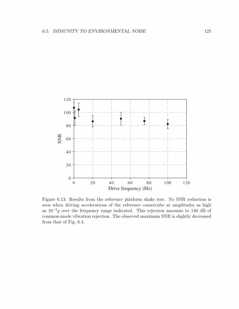
6.5. IMMUNITY TO ENVIRONMENTAL NOISE 125
0 20 40 60 80 100 1200
20
40
60
80
100
120
Drive frequency (Hz)
SNR
Figure 6.13: Results from the reference platform shake test. No SNR reduction isseen when driving accelerations of the reference cornercube at amplitudes as highas 10−2g over the frequency range indicated. This rejection amounts to 140 dB ofcommon-mode vibration rejection. The observed maximum SNR is slightly decreasedfrom that of Fig. 6.4.
126 CHAPTER 6. RESULTS
Vibration Frequency (Hz)
0.01 0.1 1 10
Ave
rage
Pha
se N
oise
(ar
b. u
nits
)
0.0001
0.001
0.01
0.1
1
10
100
1000
Figure 6.14: Average vibrational phase noise of a given frequency for an interferometerof time T = 153 ms as a function of a platform’s vibrations at discrete frequenciesand a fixed amplitude.
6.5. IMMUNITY TO ENVIRONMENTAL NOISE 127
simulation was performed by using the theory of section 4.4 to calculate the phase
shift induced by a platform acceleration a = asin(ωt). The resulting phase noise was
averaged over the relative phase of the driving signal with the interferometer pulse
timing. The impact of vibrational noise falls off as 1/ω2. It was found that if vibra-
tions of a specific, well-defined frequency are present, then it should be possible to
remove their effect entirely by choosing an interferometer time to alias the vibrations.
6.5.2 Rotation
Tilts of the Raman interferometer beams are expected to degrade the sensitivity of
the measurement. In order to study the effects of small tilt displacements, the optical
table on which the gradiometer apparatus was mounted was floated using commercial
pneumatic legs (Newport I-2000). Tilt motions were driven with an appropriately
placed voice coil and characterized using a tilt meter (Applied Geomechanics 755-
1129; specified resolution of 1 µrad, 20 Hz bandwidth). The rotation vector associated
with the tilt motion was in a plane perpendicular to the Raman propagation axis,
and the center of rotation was approximately 2 m for the accelerometers. Fig. 6.15
shows observed SNR versus maximum tilt amplitude for different driving frequencies.
Gaussian elimination was used to reduce this data. At higher frequencies, the massive
optical table could not be driven with large tilt amplitudes, and the data could not
be extended past 10 µrad.
Both centrifugal and Coriolis forces lead to a degradation in instrument sensitivity.
A rotation Ω generates a centrifugal acceleration R Ω2, where R is the distance of
one accelerometer from the center of rotation. For two accelerometers separated by
distance δR, the differential acceleration is δR Ω2, while the acceleration gradient is
Ω2. For our operating parameters, we expect this mechanism to begin to degrade the
SNR at Ω ∼ 10−4 rad/s. However, full loss in SNR is not expected until Ω ∼ 10−3
rad/s for this mechanism, much higher than the rotation rates employed in this study.
However, the Coriolis force leads to a loss in fringe contrast. In this case, the source
transverse velocity spread of δv ∼ 3 cm/s leads to an interference phase spread of
δφ ∼ 2keffδvΩT 2. At Ω ∼ 10−4, δφ ∼ 1 rad, a full loss in contrast is expected. This
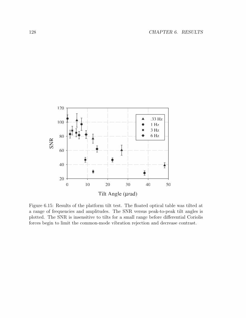
128 CHAPTER 6. RESULTS
Tilt Anggle (µµrad)
0 10 20 30 40 50
SNR
20
40
60
80
10
120
.33 Hz1 Hz3 Hz6 Hz
Figure 6.15: Results of the platform tilt test. The floated optical table was tilted ata range of frequencies and amplitudes. The SNR versus peak-to-peak tilt angles isplotted. The SNR is insensitive to tilts for a small range before differential Coriolisforces begin to limit the common-mode vibration rejection and decrease contrast.
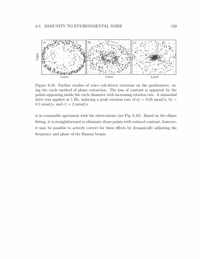
6.5. IMMUNITY TO ENVIRONMENTAL NOISE 129
Lower
Upp
er
Lower Lower
a) b) c)
Figure 6.16: Further studies of voice coil-driven rotations on the gradiometer, us-ing the circle method of phase extraction. The loss of contrast is apparent by thepoints appearing inside the circle diameter with increasing rotation rate. A sinusoidaldrive was applied at 1 Hz, inducing a peak rotation rate of a) ∼ 0.05 mrad/s, b) ∼0.5 mrad/s, and c) ∼ 2 mrad/s.
is in reasonable agreement with the observations (see Fig. 6.16). Based on the ellipse
fitting, it is straightforward to eliminate those points with reduced contrast, however,
it may be possible to actively correct for these effects by dynamically adjusting the
frequency and phase of the Raman beams.
Chapter 7
Discussion
Improvements to the gradiometer have allowed a new level of sensitivity and accuracy
to be reached. The new results demonstrate this performance and also probe impor-
tant technical aspects of the device which allow strong suppression of vibrational
noise. In this section, limitations of the current device are discussed. A method
of enhancing the sensitivity with the use of multiple Raman pulses is described and
demonstrated. Additionally, a comparison is made with several different types of atom
interferometers capable of sensing gradients. Finally, several different configurations
for measuring the full gradient tensor are described.
7.1 Performance Limits
7.1.1 SNR limits
For the T = 157.5 ms gradiometer, the demonstrated SNR is predominantly limited
by atom number shot noise. With the current signal levels, the photon shot noise
limit from unabsorbed light is close as well. The fringe amplitude corresponds to
about 2.5× 10⁵ atoms, and at the typical 33% fringe contrast, there is a mean offset
of 7 × 10⁵ atoms. Based on atom shot noise, these atom numbers put a limit of
300:1 on the SNR for each interference fringe[2.5 × 10⁵/(7 × 105)1/2
]. Additionally,
adding in the uncorrelated noise from a second trace by normalizing each chamber
130
7.1. PERFORMANCE LIMITS 131
reduces the SNR for each gravimeter to (300/21/2):1. Simultaneously using the two
gravimeter signals to produce a gradient signal decreases the SNR by another factor
of 21/2, fundamentally limiting the SNR for the full gravity gradiometer to 150:1.
This places an upper limit on the sensitivity for a 10 m device of 4 E/Hz1/2, when
the data collection time (typically 1.4 s per shot) and wild data point reduction are
included. The noise produced from photon shot noise on the unabsorbed portion of
the probe detection light, ∼ 325 atom minimum detectable signal, is approximately
at the 800:1 level for each individual fringe, giving about a 400:1 limit after the
normalization and subtraction of the two fringes. This means that photon shot noise
does not impose a substantial SNR limit for the current number of atoms, but it
would become significant for reduced atom numbers.
Improvements to the system could further increase the sensitivity. A larger num-
ber of atoms in the interferometer may be possible with improved optical pumping
techniques in the state selection or possibly starting with colder atoms to lessen the
loss of signal due to ballistic expansion. An increase of four times in the atom num-
ber would correspond to an increase in sensitivity to 2 E/Hz1/2. Additionally, use of
the molasses beams to stop and hold the atoms during detection may make longer
integration possible, which should further reduce the background noise on the signal.
With a ten times longer detection integration, photon shot noise would be reduced
by a factor of three, which would make the photon shot noise negligible even with
fewer atoms. Another promising approach is the use of multiple pulse interferometers
which have been demonstrated [100]. Multiples pulses result in larger momentum
transfer to the atoms which leverages the sensitivity up. This technique is described
in section 7.2.1. Extending an interferometer with 6hk wavepacket splitting to the
current setup with a T = 157.5 ms interferometer would push the sensitivity below 1
E/Hz1/2, when used in conjunction with greater atom numbers.
7.1.2 Rotations
Another, less fundamental, potential problem with the gradiometer concerns rota-
tions. Rotations are detrimental to the gradiometer’s performance for several reasons.
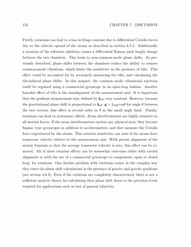
132 CHAPTER 7. DISCUSSION
Firstly, rotations can lead to a loss in fringe contrast due to differential Coriolis forces
due to the velocity spread of the atoms as described in section 6.5.2. Additionally
a rotation of the reference platform causes a differential Raman path length change
between the two chambers. This leads to non-common-mode phase shifts. As pre-
viously described, phase shifts between the chambers reduce the ability to remove
common-mode vibrations, which limits the sensitivity in the presence of tilts. This
effect could be accounted for by accurately measuring the tilts, and calculating the
tilt-induced phase shifts. In this manner, the common mode vibrational rejection
could be regained using a commercial gyroscope in an open-loop fashion. Another
harmful effect of tilts is the misalignment of the measurement axis. It is important
that the gradient measurement axis, defined by keff, stay constant. However, because
the gravitational phase shift is proportional to keff ·g = keffg cosθ for angle θ between
the two vectors, this effect is second order in θ in the small angle limit. Finally,
rotations can lead to systematic offsets. Atom interferometers are highly sensitive to
all inertial forces. If the atom interferometers enclose any physical area, they become
Sagnac type gyroscopes in addition to accelerometers, and they measure the Coriolis
force experienced by the atoms. This rotation sensitivity can arise if the atoms have
transverse velocity relative to the measurement axis. With precise alignment of the
atomic fountain so that the average transverse velocity is zero, this effect can be re-
moved. All of these rotation effects can be somewhat overcome either with careful
alignment or with the use of a commercial gyroscope to compensate, open or closed
loop, for rotations. One further problem with rotations comes in the complex way
they enter the phase shift calculations in the presence of gravity and gravity gradients
(see section 4.6.3). Even if the rotations are completely characterized, there is not a
sufficient analytic theory for calculating their phase shift down to the precision levels
required for applications such as test of general relativity.
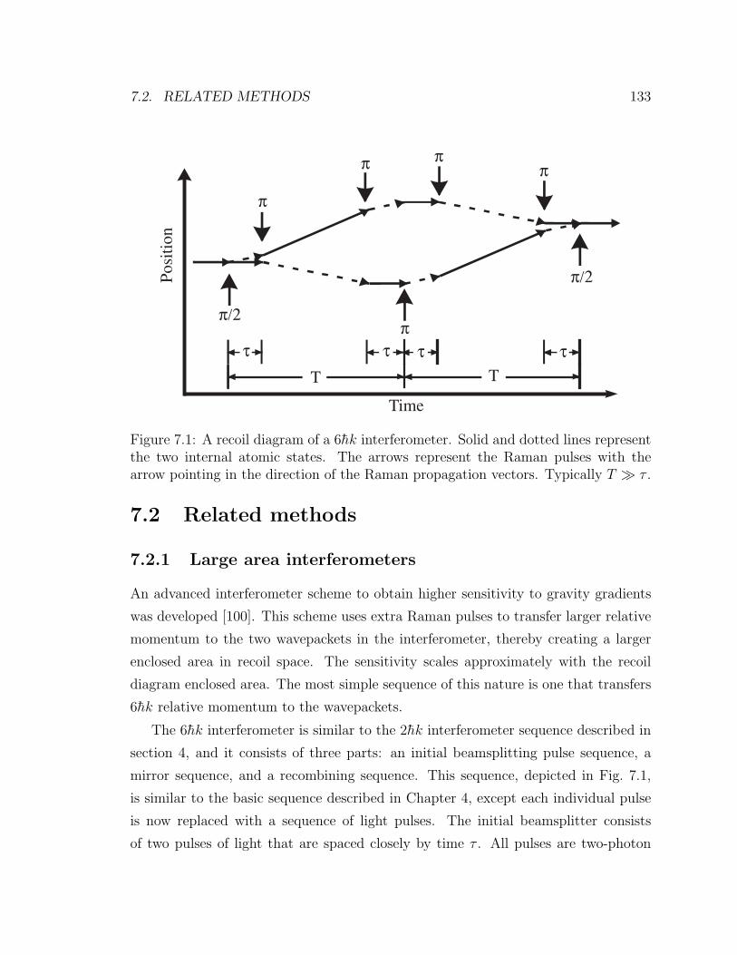
7.2. RELATED METHODS 133
Posi
tion
TT
π
π
ππ
π
π/2
π/2
τ τ τ τ
Time
Figure 7.1: A recoil diagram of a 6hk interferometer. Solid and dotted lines representthe two internal atomic states. The arrows represent the Raman pulses with thearrow pointing in the direction of the Raman propagation vectors. Typically T τ .
7.2 Related methods
7.2.1 Large area interferometers
An advanced interferometer scheme to obtain higher sensitivity to gravity gradients
was developed [100]. This scheme uses extra Raman pulses to transfer larger relative
momentum to the two wavepackets in the interferometer, thereby creating a larger
enclosed area in recoil space. The sensitivity scales approximately with the recoil
diagram enclosed area. The most simple sequence of this nature is one that transfers
6hk relative momentum to the wavepackets.
The 6hk interferometer is similar to the 2hk interferometer sequence described in
section 4, and it consists of three parts: an initial beamsplitting pulse sequence, a
mirror sequence, and a recombining sequence. This sequence, depicted in Fig. 7.1,
is similar to the basic sequence described in Chapter 4, except each individual pulse
is now replaced with a sequence of light pulses. The initial beamsplitter consists
of two pulses of light that are spaced closely by time τ . All pulses are two-photon
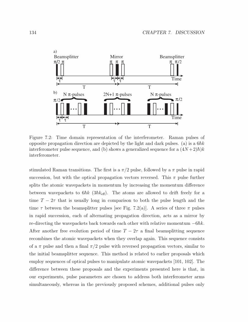
134 CHAPTER 7. DISCUSSION
//2 π π π π π /2
τ τ
π
τ
MirrorBeamsplitter Beamsplitter
T T
Time
π
π //2
τ τ
2N+1 π-pulses N π-pulsesN π-pulses
T T
Time
π//2 b)
a)
Figure 7.2: Time domain representation of the interferometer. Raman pulses ofopposite propagation direction are depicted by the light and dark pulses. (a) is a 6hkinterferometer pulse sequence, and (b) shows a generalized sequence for a (4N+2)h)kinterferometer.
stimulated Raman transitions. The first is a π/2 pulse, followed by a π pulse in rapid
succession, but with the optical propagation vectors reversed. This π pulse further
splits the atomic wavepackets in momentum by increasing the momentum difference
between wavepackets to 6hk (3hkeff). The atoms are allowed to drift freely for a
time T − 2τ that is usually long in comparison to both the pulse length and the
time τ between the beamsplitter pulses [see Fig. 7.2(a)]. A series of three π pulses
in rapid succession, each of alternating propagation direction, acts as a mirror by
re-directing the wavepackets back towards each other with relative momentum −6hk.
After another free evolution period of time T − 2τ a final beamsplitting sequence
recombines the atomic wavepackets when they overlap again. This sequence consists
of a π pulse and then a final π/2 pulse with reversed propagation vectors, similar to
the initial beamsplitter sequence. This method is related to earlier proposals which
employ sequences of optical pulses to manipulate atomic wavepackets [101, 102]. The
difference between these proposals and the experiments presented here is that, in
our experiments, pulse parameters are chosen to address both interferometer arms
simultaneously, whereas in the previously proposed schemes, additional pulses only
7.2. RELATED METHODS 135
address one arm of the interferometer at a time.
To derive the acceleration induced phase shift for the 6hk interferometer, the
rules outlined in section 3.7 for two-photon stimulated Raman transitions are applied
similarly to section 4.4. Performing this calculation for the seven pulse sequence gives:
∆φ = [φ(t1) + 2φ(t2)] − 2 [φ(t3) + φ(t4) + φ(t5)] + [2φ(t6) + φ(t7)] . (7.1)
The three quantities in brackets correspond to the phase imparted to the atoms by the
initial beamsplitting pulses, the mirror pulses and the recombining pulses respectively.
Here ti is the time of the ith pulse, and φ(ti) = keff ·x(ti)+φi are the effective phases of
the laser fields at the positions x(ti). The positions x(ti) are evaluated with respect
to the classical trajectories associated with the atomic wavepackets, and φi is the
phase reference for the ith pulse and is taken to be zero for these calculations (see
section 4.4.2). Finally, the smaller terms in the total phase from the free propagation
of the atoms and the final wavepacket overlap are neglected here1. This expression
simplifies to:
∆φ = 3keff · gT 2 − 4keff · gTτ. (7.2)
In our geometry, this becomes:
∆φ 6kgT 2 − 8kgTτ, (7.3)
where keff 2k. This shift is approximately three times the phase shift expected from
a π/2 − π − π/2 pulse sequence for long interrogation times T . The area enclosed
by interfering wavepacket trajectories has increased by the same factor2. It is stated
without proof that the sensitivity of a Raman pulse-type interferometer scales linearly
with recoil diagram area, to first order.
The Raman propagation vector reversal is achieved by means of the Pockels cell.
Adjusting the voltage applied to the Pockels cell simultaneously rotates the polar-
ization of the orthogonally polarized Raman beams. This is done exactly as in the
1These two terms are treated exactly as in the 2hk case.2There is no physical area enclosed, only area in the recoil diagram.
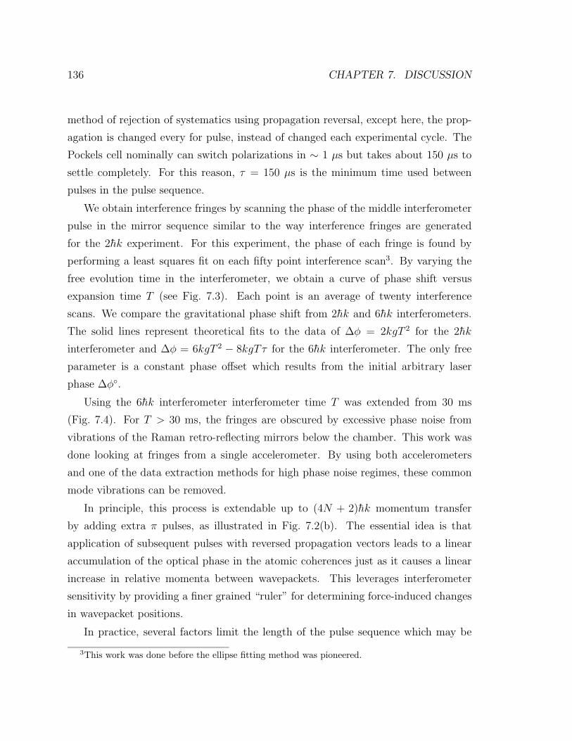
136 CHAPTER 7. DISCUSSION
method of rejection of systematics using propagation reversal, except here, the prop-
agation is changed every for pulse, instead of changed each experimental cycle. The
Pockels cell nominally can switch polarizations in ∼ 1 µs but takes about 150 µs to
settle completely. For this reason, τ = 150 µs is the minimum time used between
pulses in the pulse sequence.
We obtain interference fringes by scanning the phase of the middle interferometer
pulse in the mirror sequence similar to the way interference fringes are generated
for the 2hk experiment. For this experiment, the phase of each fringe is found by
performing a least squares fit on each fifty point interference scan3. By varying the
free evolution time in the interferometer, we obtain a curve of phase shift versus
expansion time T (see Fig. 7.3). Each point is an average of twenty interference
scans. We compare the gravitational phase shift from 2hk and 6hk interferometers.
The solid lines represent theoretical fits to the data of ∆φ = 2kgT 2 for the 2hk
interferometer and ∆φ = 6kgT 2 − 8kgTτ for the 6hk interferometer. The only free
parameter is a constant phase offset which results from the initial arbitrary laser
phase ∆φ.
Using the 6hk interferometer interferometer time T was extended from 30 ms
(Fig. 7.4). For T > 30 ms, the fringes are obscured by excessive phase noise from
vibrations of the Raman retro-reflecting mirrors below the chamber. This work was
done looking at fringes from a single accelerometer. By using both accelerometers
and one of the data extraction methods for high phase noise regimes, these common
mode vibrations can be removed.
In principle, this process is extendable up to (4N + 2)hk momentum transfer
by adding extra π pulses, as illustrated in Fig. 7.2(b). The essential idea is that
application of subsequent pulses with reversed propagation vectors leads to a linear
accumulation of the optical phase in the atomic coherences just as it causes a linear
increase in relative momenta between wavepackets. This leverages interferometer
sensitivity by providing a finer grained “ruler” for determining force-induced changes
in wavepacket positions.
In practice, several factors limit the length of the pulse sequence which may be
3This work was done before the ellipse fitting method was pioneered.
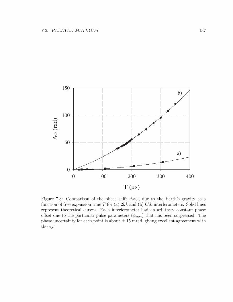
7.2. RELATED METHODS 137
T (µs)
0 100 200 300 400
∆φ (
rad )
0
50
100
150b)
a)
Figure 7.3: Comparison of the phase shift ∆φtot due to the Earth’s gravity as afunction of free expansion time T for (a) 2hk and (b) 6hk interferometers. Solid linesrepresent theoretical curves. Each interferometer had an arbitrary constant phaseoffset due to the particular pulse parameters (φlaser) that has been surpressed. Thephase uncertainty for each point is about ± 15 mrad, giving excellent agreement withtheory.
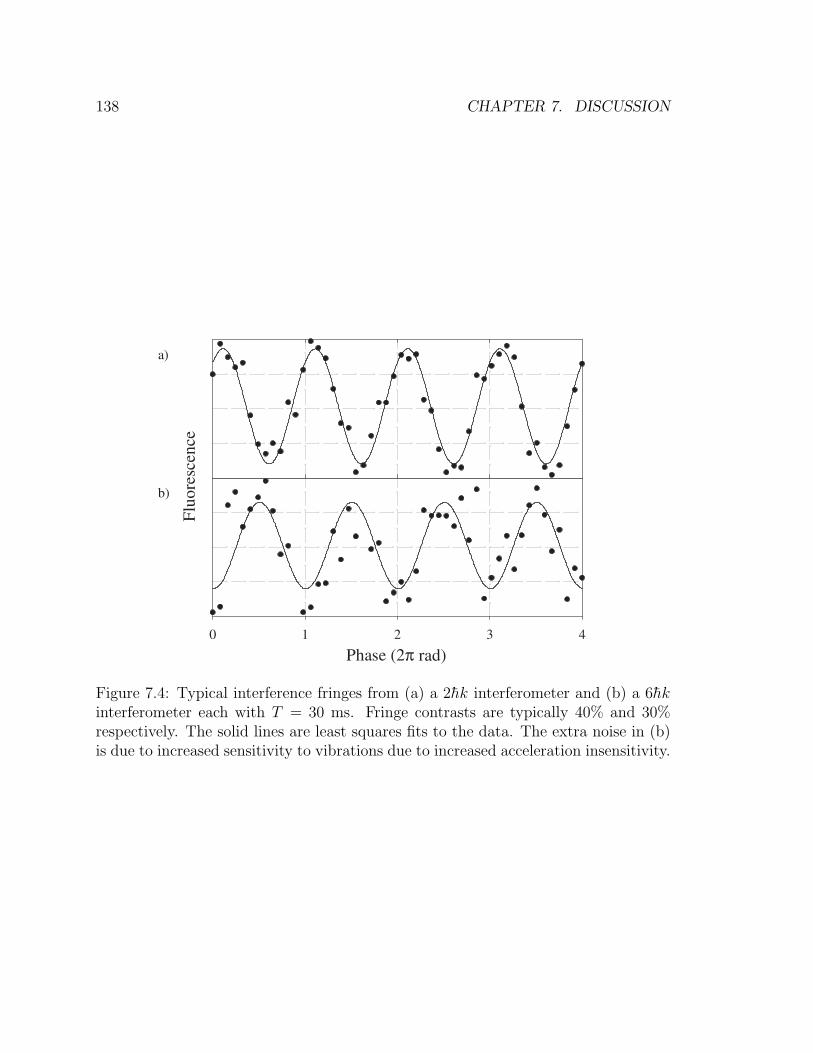
138 CHAPTER 7. DISCUSSION
Phase (2π rad)0 1 2 3 4
Flu
ores
cenc
e
a)
b)
Figure 7.4: Typical interference fringes from (a) a 2hk interferometer and (b) a 6hkinterferometer each with T = 30 ms. Fringe contrasts are typically 40% and 30%respectively. The solid lines are least squares fits to the data. The extra noise in (b)is due to increased sensitivity to vibrations due to increased acceleration insensitivity.
7.2. RELATED METHODS 139
used. First, spontaneous emission during the Raman transitions due to weak coupling
to the allowed single-photon transitions to the intermediate state homogenously de-
phases the atomic coherence and places a lower limit on the optical detuning for the
Raman pulses. This places an upper limit on the two-photon Rabi frequency, thereby
limiting the velocity class of atoms selected by the pulses. For our parameters, we
experience 1% spontaneous emission for each π pulse. Second, the Gaussian spa-
tial profile of the Raman beams leads to an inhomogeneous distribution of effective
Rabi frequencies. This introduces a spread in pulse area across the atomic spatial
distribution and ultimately limits the ensemble transfer efficiency of each π pulse.
Additionally, the frequency selectivity of the interrogating pulses limits the number
of pulses in the sequence, as the linewidth of each pulse needs to accommodate the
differential Doppler shifts in the transition frequencies due to the recoil momentum
imparted to the atomic wavepackets by previous pulses. Finally, due to the ineffi-
ciencies mentioned, less than perfectly efficient pulses can lead to a superposition of
interferometers, e.g . wavepackets following both a 2hk and a 6hk loop at the same
time, resulting in an averaging of the phase shifts for the two interferometer loops.
We are exploring methods to overcome the above limitations to realize high mo-
mentum transfer atom optics. There do not appear to be any serious barriers to
realization of momentum transfers greater than 10hk. Such high momentum beam-
splitters would offer new levels of sensitivity for atom interferometer based precision
measurements.
7.2.2 Interferometer comparisons
There have been several investigations of gravimeters with different types of atom in-
terferometers. These include atom interferometers based on multiple pulse techniques
using stimulated Raman transitions (see section 7.2.1), Bragg scattering, diffraction in
the Raman-Nath regime, adiabatic transfer, and the AC Josephson effect with Bose-
Einstein condensates (BEC). The advantages and disadvantages of each technique
will be discussed here.
The 6hk interferometer should prove to be a sensitive gradient sensing tool. This
140 CHAPTER 7. DISCUSSION
method might be extended even further using special sequences of composite pulses
(see section 5.5.2). The benefits of using composite pulses in this context would be
an large range of selected velocities for a fixed Rabi frequency and robust suppression
of spatial inhomogeneities in Rabi frequency (which arise due to the spatial intensity
profile of the gaussian Raman laser beams). For example, consider the following se-
quence. A high efficiency composite microwave pulse could be used for the initial π/2
pulse. Next a composite optical π pulse gives the wavepackets 4hk momentum split-
ting, and after a long drift time two composite π pulses redirect the wavepackets back
towards each other. Finally, a last composite optical pulse and another composite mi-
crowave pulse recombine the wavepackets to complete the interferometer. Because it
uses coupled composite pulses, simulations have shown that this interferometer could
result in extremely high contrast interference fringes due to its increased insensitivity
to inhomogeneous broadening.
Bragg scattering-based interferometers diffract atoms from standing waves of laser
light. As in the light-pulse interferometers, these interactions can be configured as
atom optic beamsplitters and mirrors [103]. The primary virtue of Bragg scattering
interferometers is that the atoms always remain in the same internal state. The
effects of many systematic phase shifts such as Zeeman shifts and AC Stark shifts are
reduced, since the wavepackets in each arm of the interferometer experience symmetric
phase shifts due to these effects. In comparison, the Raman method requires the use of
propagation vector reversal techniques to gain immunity to these possible systematics.
Furthermore, high-order Bragg diffraction can be used to create large-area, high-
sensitivity instruments. However, high-order Bragg processes only operate efficiently
over a relatively narrow range of initial atomic velocities (significantly less than a
photon recoil velocity). This severely constrains the fraction of atoms which can
contribute to the interference signal, and thus the sensitivity drops due to small atom
counting rates. On the other hand, BEC or atom laser sources may eventually produce
extremely bright atomic beams (having excellent velocity collimation) [55, 104]. In
this case, Bragg processes may become a competitive choice for interferometer sensors,
however it is unlikely that robust condensates will be developed in the near future.
7.2. RELATED METHODS 141
A gravimeter based on diffraction in the Raman-Nath regime has also been demon-
strated [105]. In this interferometer, short, intense pulses of highly focused light are
applied to the atom. Because of the short pulse and tight focus, atoms are diffracted
into a large spread of momentum states, with many multiples of 2hk present. Two
Raman-Nath pulses are used to construct the interferometer, and because of the wide
spread of momentum, many different interfering paths exist. Some of these paths
overlap and interfere after an echo time, which determines the sensitivity to gravita-
tional phase shifts. The many paths increase the finesse of the interference fringes and
provide greater ability to resolve phase shifts than for single path interferometers for
identical SNRs. This sensitivity scales with increasing echo time. However, Raman-
Nath diffraction populates many higher lying momentum states that do not contribute
to the closed interferometer paths, which decreases the interferometer contrast and
limits the SNR by limiting the counting statistics. A comparison is given between
the gravitational phase shift in a Raman interferometer and a Raman-Nath interfer-
ometer, based on the theoretical treatment in [105]. For equal total interferometer
time (N + 1)T , the ratio of of the Raman-Nath phase shift, keff · gT 2N(N + 1)/2 for
the N th echo, to the Raman phase shift, keff ·gT 2(N +1)2/4, is given by 2N/(N +1).
The maximum theoretical interferometer contrast is used as a weighting factor here:
100% for Raman interferometers and for Raman-Nath devices the maximum of JN and
JN+1 for the N th echo where JN is a first order Bessel function. Because of the severe
drop in contrast for Raman-Nath beamsplitters, the maximum effective momentum
transfer is only approximately 0.5hk when after the decreased counting statistics are
included, which is twelve times less sensitive than a 6hk Raman-type interferometer.
Additionally, if the shot noise from the atoms in momentum states not contributing
to the signal is considered, the Raman-Nath interferometer is 42 times less sensitive
than a 6hk Raman interferometer. This relative sensitivity becomes even worse for
higher order Raman beamsplitters, e.g. 10hk and higher. Even with an ultra-cold
source, sensitive Raman-Nath gravimeters and gradiometers seem infeasible.
Adiabatic transfer recently has been used in a proof-of-principle demonstration of a
possible large-area interferometer [106]. In this approach, atoms are put into coherent
superpositions of two states using a microwave pulse. Momentum is transferred to one
142 CHAPTER 7. DISCUSSION
state in this superposition by adiabatically transferring it from the mF = 0 sublevel
to the highest (or lowest) lying mF level [51]. Adiabatic transfer is used subsequently
to manipulate and ultimately to overlap the wavepackets. A final microwave pulse
is then used to interfere these wavepackets. This method can transfer up to 2mF hk
momentum to one arm of the interferometer. The primary limitation to the utility of
this method is that the adiabatic transfer populates magnetic field sensitive sublevels.
This makes the interferometer sensitive to Zeeman shifts, e.g. a 1 mG difference in
field between two 150 ms interferometers in a gradiometer produces a phase change
of ∼ 30 rad, which is similar in size to a change of 2.5 × 10⁻⁶g. While such an
interferometer may demonstrate a high sensitivity, it remains to be seen whether it
can achieve high accuracy.
Finally, the AC Josephson effect in arrays of Bose-Einstein condensed atoms [107]
has been used to make a proof-of-principle gravity measurement. In this approach,
condensate atoms tunnel from an array of vertically spaced lattice sites. Atoms tun-
nelling from different sites subsequently interfere. The resulting interference pattern
is a periodic train of atom pulses whose frequency depends on the strength of the
gravitational potential. This frequency can be measured with high accuracy using
conventional atom detection techniques. A major technological drawback to this
technique is the need for Bose-Einstein condensed atomic sources, which still are dif-
ficult to produce and not suitable for a portable apparatus. Also, the time required
to condense atoms is typically in excess of 30 s, which results in a low instrument
bandwidth. However, if techniques to produce robust, BEC atom sources improve,
this method may become viable for future instruments.
7.2.3 Multi-loop interferometers
There are several Raman-pulse based schemes which can be used for direct gravity
gradient measurements. The simplest of these is the double-loop, or figure-eight,
interferometer which was first proposed in [12]. This geometry can be easily achieved
in the light-pulse method by inserting an extra π pulse into the light-pulse sequence.
Instead of applying a π/2 pulse for the third pulse, the two atomic wavepackets are
7.2. RELATED METHODS 143
allowed to pass through each other and form a second loop [see Fig. 7.5b]. Next
a second π pulse redirects the wavepackets to close the second loop, and a final
π/2 pulse interferes the wavepackets. This pulse sequence directly produces a phase
shift proportional to the the gravity gradient by essentially performing a coherent
subtraction of two spatially, and temporally, separated gravity measurements (one
for each loop). Following the pulse rules presented in section 4.4, the double-loop
phase shift is given by:
∆φ φ(t1) − 2φ(t2) + 2φ(t3) − φ(t4), (7.4)
where φ(ti) is the phase of the ith Raman pulse at the position of the atomic wave-
packet at time ti. Evaluating this phase, assuming a linear gravitational gradient
g(z) = g + αz along the sensitive axis, gives:
∆φ 8kgαT 4, (7.5)
where g is the gravitational component along the Raman wavevector at the atoms’
initial position and α is the linear gradient. This formula is valid for an interferometer
in the first half of a fountain of length 8T and for αz′ g where z′ is the total height
of the fountain.
One problem with this approach is that, for a given fountain height, the double-
loop interferometer is maximally sensitive when the interferometer occurs in only one
half of the fountain. If the interferometer spans the whole fountain time, i.e. is
symmetric about the fountain’s peak, then the gravity signal from each loop will be
identical, resulting in no phase shift. Thus, to obtain gradient sensitivity, the double-
loop must be used only in the first half or the second half of the fountain, which
severely constrains the possible instrument sensitivity. (This means the maximum
interaction time for our fountain is T = 39 ms, resulting in 3000 times less sensitivity
to gradients as compared with two single loop interferometer which are separated
by 10 m.) In addition to this sensitivity limit, it is difficult to make the gradiometer
baseline arbitrarily large and there is no common-mode vibration rejection, since each
of the two acceleration measurements which comprise the gravity gradient signal are
144 CHAPTER 7. DISCUSSION
Time
(a)
Dis
tance
Alo
ng R
aman
Las
er B
eam
s
(c)
(b)
(1+ 2 )T (1+ 2 )T
π π/2
π/2π
T T
π/2 πT 2T
π π/2π/2 π πT
T
T
π/2
Figure 7.5: Recoil diagrams for various interferometer sequences. Solid and dottedlines represent the F = 3 and F = 4 states respectively. The time of the Raman pulsesis denoted by the vertical arrows. a) Single-loop accelerometer. b) Double-loop (figureeight) gradiometer. c) Triple-loop gradiometer.
7.2. RELATED METHODS 145
made at differing times.
A slight modification of the double-loop method allows full use of the fountain
interaction time, resulting in a three-fold increase in sensitivity from a double-loop
interferometer in an apparatus of equivalent size. This modified sequence uses an
extra π pulse in a π/2 − π − π − π − π/2 sequence, which creates a triple-loop
interferometer as seen in Fig. 7.5(c). The phase shift is:
∆φ φ(t1) − 2φ(t2) + 2φ(t3) − 2φ(t4) + φ(t5), (7.6)
which reduces to:
∆φ (
17
3+ 4
√2)kgαT 4, (7.7)
again assuming a linear gradient and an interferometer that now spans the entire
fountain time, (8 + 4√
2)T . This interferometer may be symmetrically spaced about
the fountain’s apex, so that the maximal interrogation time is T = 46 ms for our
fountain. Typical interference fringes from a triple loop interferometer are shown
in Fig. 7.6. The 10 m single-loop, two chamber gradiometer still is 1000 times more
sensitive due to its larger baseline and longer effective interrogation time. In addition,
the triple-loop gradiometer, like the double-loop, does not provide vibration rejection,
has a limited baseline, and is only slightly less sensitive to magnetic fields.
7.2.4 Curvature measurements
Two multiple-loop gradiometers may be used in conjunction to measure the second
moment of the gravity field, in a configuration similar to that used to measure the
gradient with two single loop interferometers, except with a triple-loop interferometer
performed on each atom ensemble. In this case, the triple-loop gradient phase shifts
obtained from two spatially separated atomic ensembles are subtracted to obtain the
second order curvature of the gravitational field. This device does have immunity
to spurious vibrational noise because measurements are made simultaneously with
respect to a common platform. Proof-of-principle data is shown in Fig. 7.6. Measure-
ment of the second moment of the gravitational field allows differentiation between
146 CHAPTER 7. DISCUSSION
Phase (2π rad)
0 1 2 3 4
Tra
nsiti
on p
roba
bilit
y (a
rb. u
nits
)
0.0
0.5
1.0
1.5
2.0
Figure 7.6: Typical interference fringes from T = 44 ms triple-loop interferometersin the lower and upper chamber. The solid lines are least squares fits, and the phasedifference between the two fringes represents a measurement of the second momentof the gravitational field.
massive, distant objects and less massive, nearby objects that a gradiometer could
not distinguish.
A more direct and sensitive way to characterize the second order moment is to
operate simultaneously three single-loop accelerometers spaced equidistantly along a
single axis. The difference between gradients obtained by differencing the first and
second accelerometer outputs from the second to third accelerometer outputs gives
a second moment measurement. This device should have the same benefits as the
previous device and would be significantly more sensitive. The disadvantage of such
a system is the added size and complexity of a third accelerometer.
7.2.5 Multi-axis gradiometers
Lastly, it is desirable to measure the entire gravity gradient tensor rather than just
a single component as the gradiometer presented here does. By doing so, the gravity
field may be more thoroughly characterized, and a better picture of the surrounding
7.2. RELATED METHODS 147
Figure 7.7: Configuration of four accelerometers for a full gradient tensor measure-ment. Two of the Raman beam paths, each defining a single tensor componentmeasurement, are shown with the arrows.
mass distribution can be obtained. There are several such accelerometer configura-
tions that would be capable of measuring the full tensor. Recall, from section 2.1, that
there are only five independent components to the gravity gradient tensor, and thus
only five orthogonal gradient measurements need to be performed for full knowledge
of the tensor.
The most straightforward configuration for measuring the full gravity gradient
tensor requires four accelerometers in a tetrahedral pattern as shown in Fig. 7.7.
The wavevector of the Raman beams defines the sensitive axis as well as the axis
to which the spatial derivative is taken. By making five measurements with the
Raman beams oriented along different axes of the tetrahedron, five different gradient
tensor components can be measured, and thus the entire tensor know. Some of the
individual gradient measurements measure a combination of two components, but
each component can be separated by combining the five measurements. The Raman
beam measurement axis can be alternated between the different atom ensembles by
coupling the light into different fibers. The beams could be switched between the
fibers using a combination of AOMs or electro-optic prisms to route the beams. As
with the single axis device, the multi-axis gradiometer can have arbitrarily large
baselines. In the case where a stable inertial platform is available, this configuration
148 CHAPTER 7. DISCUSSION
can be simplified. In this instance, it is possible to make a full gradient tensor
measurement using only three accelerometers. This is only the case if all Raman beam
launching optics mounted to different parts of the stable platform vibrate together.
This configuration can save on the size and cost of a full tensor system.
Finally, there are more speculative methods that may be able to measure multiple
components of the gravity gradient tensor. One such method method relies on the
complete theory from Chapter 4. Included in this theory would have to be all possible
acceleration terms, including transverse gravitational accelerations and gradients, as
well as rotations. If a sufficient analytic approximation for the inertial force induced
phase shift can be found, then it may be possible to access individual terms in the
analytic expansion of the phase by varying physical parameters of the experiment.
For instance, a specific component of the gravity field might be contained in a term
that could be amplified by adjusting the interferometer time and launch velocity,
as well as perhaps inducing known rotations. It is nontrivial to derive an analytic
approximation that agrees well with the exact solution, so this approach might not be
possible. Additionally, such effects might be too small to make precise measurements
in reasonable integration times.
Chapter 8
Conclusion
We have demonstrated a precise and accurate gravity gradiometer based on light-pulse
atom interference techniques. In addition, it is the first realization of an absolute
gradiometer. The gradiometer has a differential sensitivity of 4 × 10⁻⁹ g in 1 s,
or in gradient units 4 E/√
Hz. The accuracy of the device has been shown to be
< 1 E. As verification of the sensitivity, the gravity gradient due to a small test
mass was measured. A series of tests to characterize the gradiometer in the presence
of reference platform rotations and linear accelerations was performed. A high SNR
detection system based on balanced, modulation transfer detection was constructed to
achieve the high SNRs required for precision gradiometry. A number of data reduction
methods were investigated, and an innovative method based on fitting ellipses to the
data was pioneered. This section briefly describes possible apparatus upgrades for
the gradiometer, including sensitivity and accuracy enhancements. Finally, the high
sensitivity and stability of the gravity gradiometer make possible a number of precision
measurements, several of which are discussed here.
8.1 Future enhancements
The current sensitivity is primarily limited by shot noise on the number of atoms
contributing to the signal. In order to improve this limit, the number of atoms
participating in the interferometer and being detected must be increased. At the
149
150 CHAPTER 8. CONCLUSION
present time only a small number of atoms are contributing to the signal. Although a
relatively large number of atoms is trapped (∼ 108) only a few times 105 contribute the
interference fringes. The inefficiencies are threefold. The optical pumping sequence
is not efficient, a considerable number of atoms are lost in the atomic fountain itself,
and the interference fringe contrast coupled with the velocity selection step limit the
signal size even more. Improving the signal levels is expected to improve the overall
sensitivity in a direct way.
These inefficiencies all have straightforward solutions conceptually, but the solu-
tions are not easy to implement. Improvements in the optical pumping could result
in more atoms in the desired internal state. Such improvements might include an
increase in the efficiency of each state preparation pulse, a reduction of rescattering
from the thermal background atoms by reducing the vapor pressure, or an altogether
different optical pumping scheme. The use of colder atom sources would solve a
number of problems. Notably, it would produce more atoms in the detection volume
following the atomic fountain by limiting the thermal expansion of the atomic clouds
during the fountain. Additionally, because the transverse spatial extent of the clouds
would be smaller, the atoms would see a more uniform intensity profile from the
Raman beams across the cloud, which would lead to higher fringe contrast. Finally,
the fringe contrast would rise due to the narrower longitudinal velocity spread caus-
ing less inhomogeneous broadening. This longitudinal narrowing might alleviate the
need for the velocity preselection step, again resulting in greater numbers of atoms
contributing to the signal. Such an ultra-cold fountain source has been demonstrated
based on Raman sideband cooling in a two-dimensional lattice [108, 109, 110]. Addi-
tionally, increasing the Raman laser power would allow for larger Rabi frequencies or
larger Raman beams, both of which would lead to contrast gains similar to cooling
the atoms further.
Multiple pulse interferometers (> 2hk) are a promising route to higher sensitivity.
Extending the proof-of-principle results for the 6hk interferometer of section 7.2.1
to higher momentum and demonstrating high SNRs for these interferometers would
linearly increase the sensitivity to gradients, provided that care is taken to avoid the
admixture of 2hk interferometer components as well. Additionally special sequences
8.2. FUTURE MEASUREMENTS 151
involving the advanced pulse techniques described in section 5.5.2 could enable high
contrast, large-area interferometers. The simulated sequence described in section 7.2.2
appears to be a promising route to high sensitivity gradient sensing. With a com-
bination of all of these improvements, a sensitivity of < 1 E/√
Hz seems feasible
(< 7 × 10⁻¹⁰ g/√
Hz per accelerometer).
Such a high sensitivity gravity gradiometer mandates a thorough study of its ac-
curacy. The current measurement of the gravitational constant provides one such
test of accuracy. However, because of the uncertainty in G, this characterization may
not be sufficient for ultra-precise measurements. The same holds true for additional
comparison with tidal models. Further characterization of accuracy might be best ac-
complished by comparison with other absolute gravity gradiometers. A second gravity
gradiometer unit is being constructed, and this device could be used to verify the ac-
curacy of the original gradiometer. Furthermore, the accuracy of the gradiometer is
limited by the precise knowledge of the distance between the two atom ensembles.
There are several steps that could be taken that might increase the stability of the
device, based on the philosophy that stabilizing as much as possible in the apparatus
would lessen any long-term drift which may be present. Actively stabilizing the in-
tensity of all the beams, including the trapping beams, detection beams, and Raman
beams would limit any potential fluctuations due to effect such as drifts of the launch
velocity, initial trap position, and Raman beam parameters. Finally, incorporation
of magnetic shielding would limit phase fluctuations from the second-order Zeeman
shift in the interferometer.
8.2 Future measurements
Currently underway is the measurement of the gravitational constant discussed in sec-
tion 6.4.3. The precision of the experiment is sufficient to make a part-per-thousand
measurement of the G in several days. The current limit to the measurement is the
accuracy of the test mass as well as the untested accuracy of the gradiometer at the
necessary levels. Several systematic effects are limiting the accuracy. The key effect
is magnetic field-induced phase shifts from the magnetic field of the platform used
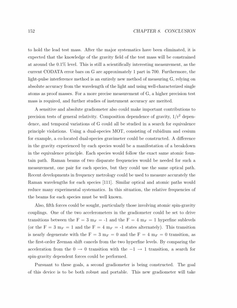
152 CHAPTER 8. CONCLUSION
to hold the lead test mass. After the major systematics have been eliminated, it is
expected that the knowledge of the gravity field of the test mass will be constrained
at around the 0.1% level. This is still a scientifically interesting measurement, as the
current CODATA error bars on G are approximately 1 part in 700. Furthermore, the
light-pulse interference method is an entirely new method of measuring G, relying on
absolute accuracy from the wavelength of the light and using well-characterized single
atoms as proof masses. For a more precise measurement of G, a higher precision test
mass is required, and further studies of instrument accuracy are merited.
A sensitive and absolute gradiometer also could make important contributions to
precision tests of general relativity. Composition dependence of gravity, 1/r2 depen-
dence, and temporal variations of G could all be studied in a search for equivalence
principle violations. Using a dual-species MOT, consisting of rubidium and cesium
for example, a co-located dual-species gravimeter could be constructed. A difference
in the gravity experienced by each species would be a manifestation of a breakdown
in the equivalence principle. Each species would follow the exact same atomic foun-
tain path. Raman beams of two disparate frequencies would be needed for such a
measurement, one pair for each species, but they could use the same optical path.
Recent developments in frequency metrology could be used to measure accurately the
Raman wavelengths for each species [111]. Similar optical and atomic paths would
reduce many experimental systematics. In this situation, the relative frequencies of
the beams for each species must be well known.
Also, fifth forces could be sought, particularly those involving atomic spin-gravity
couplings. One of the two accelerometers in the gradiometer could be set to drive
transitions between the F = 3 mF = -1 and the F = 4 mF = 1 hyperfine sublevels
(or the F = 3 mF = 1 and the F = 4 mF = -1 states alternately). This transition
is nearly degenerate with the F = 3 mF = 0 and the F = 4 mF = 0 transition, as
the first-order Zeeman shift cancels from the two hyperfine levels. By comparing the
acceleration from the 0 → 0 transition with the −1 → 1 transition, a search for
spin-gravity dependent forces could be performed.
Pursuant to these goals, a second gradiometer is being constructed. The goal
of this device is to be both robust and portable. This new gradiometer will take
8.2. FUTURE MEASUREMENTS 153
advantage of compact optics and a simplified system to achieve similar sensitivities in
a significantly smaller package. The portable gradiometer could then be used in field
tests to characterize gravity gradients from environmental mass anomalies such as
oil and minerals and subsurface structures. Additionally, it should be noted that the
performance of a gravity gradiometer in a microgravity environment would be greatly
enhanced due to the larger available interrogation time (φtot α T 2) without need
for an atomic fountain, and measurements as small as 10−15 g would be accessible.
Such a high sensitivity device would be ideal for tests of fundamental theories or for
high altitude measurements of gradients from terrain features at the Earth’s surface.
Finally, in order to perform such long interrogation time measurements, the theory
of gravitationally and rotationally-induced phase shifts in light-pulse interferometers
needs to be refined. Based on its demonstrated sensitivity and accuracy, however,
the gravity gradiometer appears poised to make important scientific contributions.
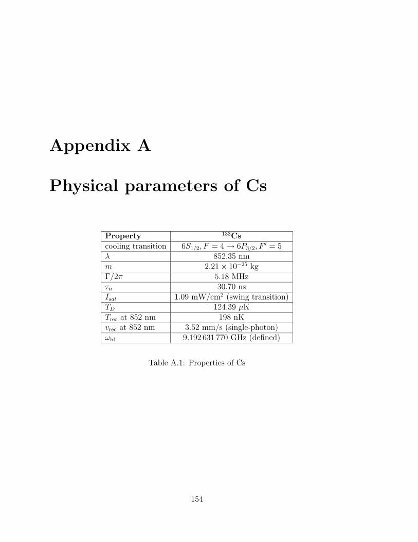
Appendix A
Physical parameters of Cs
Property 133Cscooling transition 6S1/2, F = 4 → 6P3/2, F
′ = 5λ 852.35 nmm 2.21 × 10⁻²⁵ kgΓ/2π 5.18 MHzτn 30.70 nsIsat 1.09 mW/cm2 (swing transition)TD 124.39 µKTrec at 852 nm 198 nKvrec at 852 nm 3.52 mm/s (single-photon)ωhf 9.192 631 770 GHz (defined)
Table A.1: Properties of Cs
154
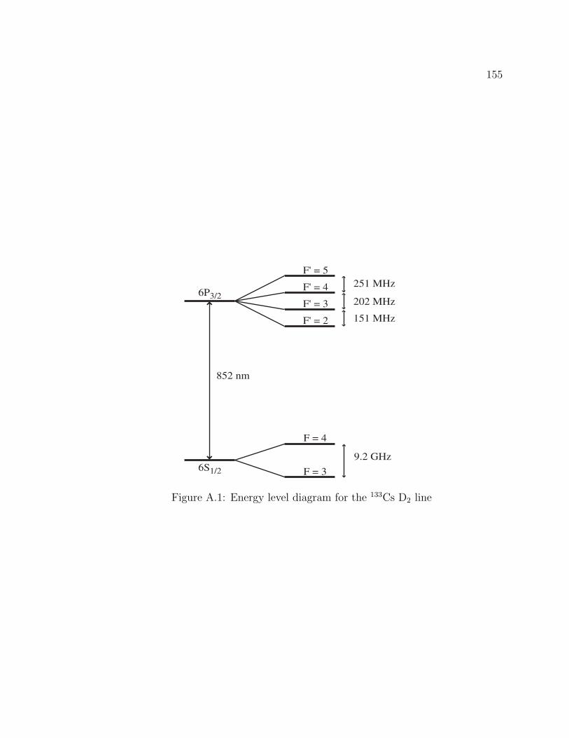
155
F' = 2
F' = 3
F' = 4
F' = 5
F = 3
F = 4
9.2 GHz
251 MHz
202 MHz
151 MHz
6P3/2
6S1/2
852 nm
Figure A.1: Energy level diagram for the 133Cs D2 line
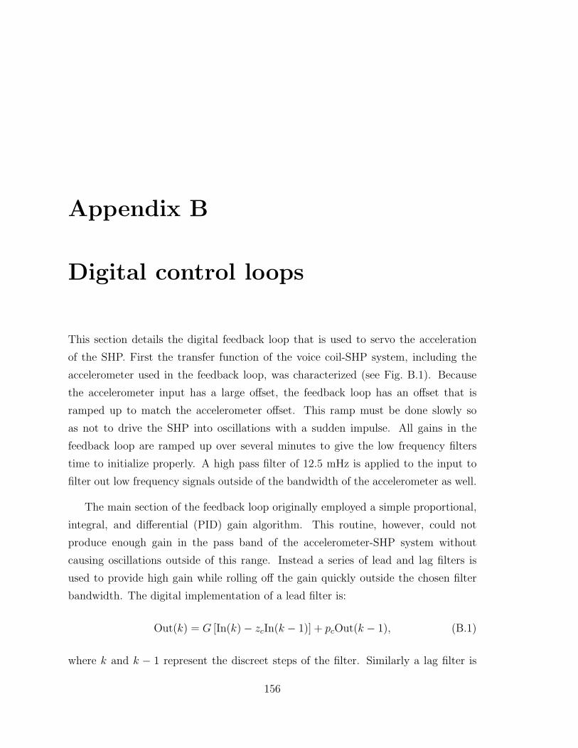
Appendix B
Digital control loops
This section details the digital feedback loop that is used to servo the acceleration
of the SHP. First the transfer function of the voice coil-SHP system, including the
accelerometer used in the feedback loop, was characterized (see Fig. B.1). Because
the accelerometer input has a large offset, the feedback loop has an offset that is
ramped up to match the accelerometer offset. This ramp must be done slowly so
as not to drive the SHP into oscillations with a sudden impulse. All gains in the
feedback loop are ramped up over several minutes to give the low frequency filters
time to initialize properly. A high pass filter of 12.5 mHz is applied to the input to
filter out low frequency signals outside of the bandwidth of the accelerometer as well.
The main section of the feedback loop originally employed a simple proportional,
integral, and differential (PID) gain algorithm. This routine, however, could not
produce enough gain in the pass band of the accelerometer-SHP system without
causing oscillations outside of this range. Instead a series of lead and lag filters is
used to provide high gain while rolling off the gain quickly outside the chosen filter
bandwidth. The digital implementation of a lead filter is:
Out(k) = G [In(k) − zcIn(k − 1)] + pcOut(k − 1), (B.1)
where k and k − 1 represent the discreet steps of the filter. Similarly a lag filter is
156
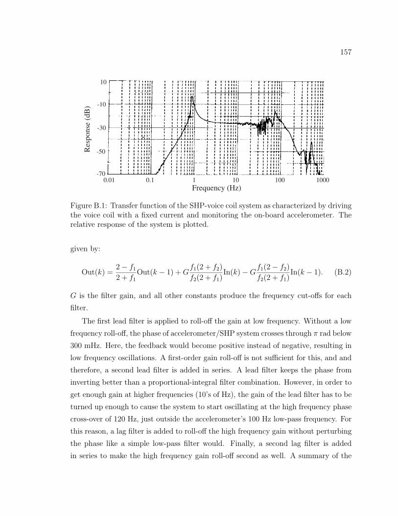
157
Frequency (Hz)
Res
pons
e (d
B)
10
-10
-30
-50
-700.01 0.1 1 10 100 1000
Figure B.1: Transfer function of the SHP-voice coil system as characterized by drivingthe voice coil with a fixed current and monitoring the on-board accelerometer. Therelative response of the system is plotted.
given by:
Out(k) =2 − f12 + f1
Out(k − 1) + Gf1(2 + f2)
f2(2 + f1)In(k) −G
f1(2 − f2)
f2(2 + f1)In(k − 1). (B.2)
G is the filter gain, and all other constants produce the frequency cut-offs for each
filter.
The first lead filter is applied to roll-off the gain at low frequency. Without a low
frequency roll-off, the phase of accelerometer/SHP system crosses through π rad below
300 mHz. Here, the feedback would become positive instead of negative, resulting in
low frequency oscillations. A first-order gain roll-off is not sufficient for this, and and
therefore, a second lead filter is added in series. A lead filter keeps the phase from
inverting better than a proportional-integral filter combination. However, in order to
get enough gain at higher frequencies (10’s of Hz), the gain of the lead filter has to be
turned up enough to cause the system to start oscillating at the high frequency phase
cross-over of 120 Hz, just outside the accelerometer’s 100 Hz low-pass frequency. For
this reason, a lag filter is added to roll-off the high frequency gain without perturbing
the phase like a simple low-pass filter would. Finally, a second lag filter is added
in series to make the high frequency gain roll-off second as well. A summary of the
158 APPENDIX B. DIGITAL CONTROL LOOPS
bandwidths and gains is found in Table B.1.
Filter Bandwidth GainLead 1 38 mHz - 200 Hz 1Lead 2 380 mHz - 200 Hz 1Lag 1 1 Hz - 80 Hz 200Lag 2 1 Hz - 80 Hz 80
Table B.1: Vibration isolation system filter bandwidths and gains.
A comparison of the lead/lag filter combination with a digital PID filter is given in
Fig B.2. The lead/lag filter combination keeps the phase constant over a larger range,
allowing the gain to be increased without driving oscillations at the phase crossover
points. Additionally, it rolls the gain off faster at low frequency.
Phas
e (r
ad)
0
π
−π
Frequency (Hz)0.01 1 1000.1 10 1000
Frequency (Hz)0.01 1 1000.1 10 1000
Gai
n (l
og a
rb. u
nits
)
0
20
40
60
80
b)
a)
a)
b)
Figure B.2: Gain and phase for a a) PID filter and b) lead/lag filter combination.
Bibliography
[1] A. Einstein, “Uber den Einfluss der Schwerkraft auf die Ausbreitung des
Lichtes,” Annalen der Physik (Leipzig) 35, 898–908 (1911).
[2] T. W. Hansch and A. L. Schawlow, “Cooling of gases by laser radiation,” Opt.
Commun. 13, 68 (1975).
[3] D. Wineland and W. Itano, Phys. Rev. A 20, 1521 (1979).
[4] W. Phillips and H. Metcalf, “Laser deceleration of an atomic beam,” Phys. Rev.
Lett. 48, 596–599 (1982).
[5] S. Chu, L. Hollberg, J. E. Bjorkholm, A. Cable and A. Ashkin, “3-Dimensional
viscous confinement and cooling of atoms by resonance radiation pressure,”
Phys. Rev. Lett. 55, 48–51 (1985).
[6] E. L. Raab, M. Prentiss, A. Cable, S. Chu and D. E. Pritchard, “Trapping of
neutral sodium atoms with radiation pressure,” Phys. Rev. Lett. 59, 2631–4
(1987).
[7] The Royal Swedish Academy of Sciences, Press Release: The 1997 Nobel Prize
in Physics (1997).
[8] N. F. Ramsey, Phys. Rev. 78, 695–9 (1950).
[9] R. Colella, A. W. Overhauser and S. A. Werner, “Observation of gravitationally
induced quantum interference,” Phys. Rev. Lett. 34, 1472–4 (1975).
159

160 BIBLIOGRAPHY
[10] S. A. Werner, J.-L. Staudenmann and R. Colella, “Effect of Earth’s rotation
on the quantum mechanical phase of the neutron,” Phys. Rev. Lett. 42, 1103–6
(1979).
[11] S. Altshuler and L. M. Frantz, “Matter wave interferometric apparatus,” U.S.
Patent 3761721 (1973).
[12] J. F. Clauser, “Ultra-high sensitivity accelerometers and gyroscopes using neu-
tral atom matter-wave interferometry,” Physica B 151, 262–72 (1988).
[13] D. W. Keith, C. R. Ekstrom, Q. A. Turchette and D. E. Pritchard, “An inter-
ferometer for atoms,” Phys. Rev. Lett. 66, 2693–6 (1991).
[14] M. Kasevich and S. Chu, “Atomic interferometry using stimulated Raman tran-
sitions,” Phys. Rev. Lett. 67, 181–4 (1991).
[15] F. Riehle, T. Kisters, A. Witte, J. Helmcke and C. J. Borde, “Optical Ramsey
spectroscopy in a rotating frame: Sagnac effect in a matter-wave interferome-
ter,” Phys. Rev. Lett. 67, 177–80 (1991).
[16] M. Kasevich and S. Chu, “Measurement of the gravitational acceleration of an
atom with a light-pulse atom interferometer,” Appl. Phys. B 54, 321–32 (1992).
[17] T. L. Gustavson, P. Bouyer and M. A. Kasevich, “Precision rotation measure-
ments with an atom interferometer gyroscope,” Phys. Rev. Lett. 78, 2046–9
(1997).
[18] A. Peters, K. Y. Chung, B. Young, J. Hensley and S. Chu, “Precision atom
interferometry,” Philos. Trans. Roy. Soc. A 355, 2223–33 (1997).
[19] M. J. Snadden, J. M. McGuirk, P. Bouyer, K. G. Haritos and M. A. Kasevich,
“Measurement of the Earth’s gravity gradient with an atom interferometer-
based gravity gradiometer,” Phys. Rev. Lett. 81, 971–4 (1998).
[20] Lorand Eotvos Virtual Museum, http://www.elgi.hu/museum.
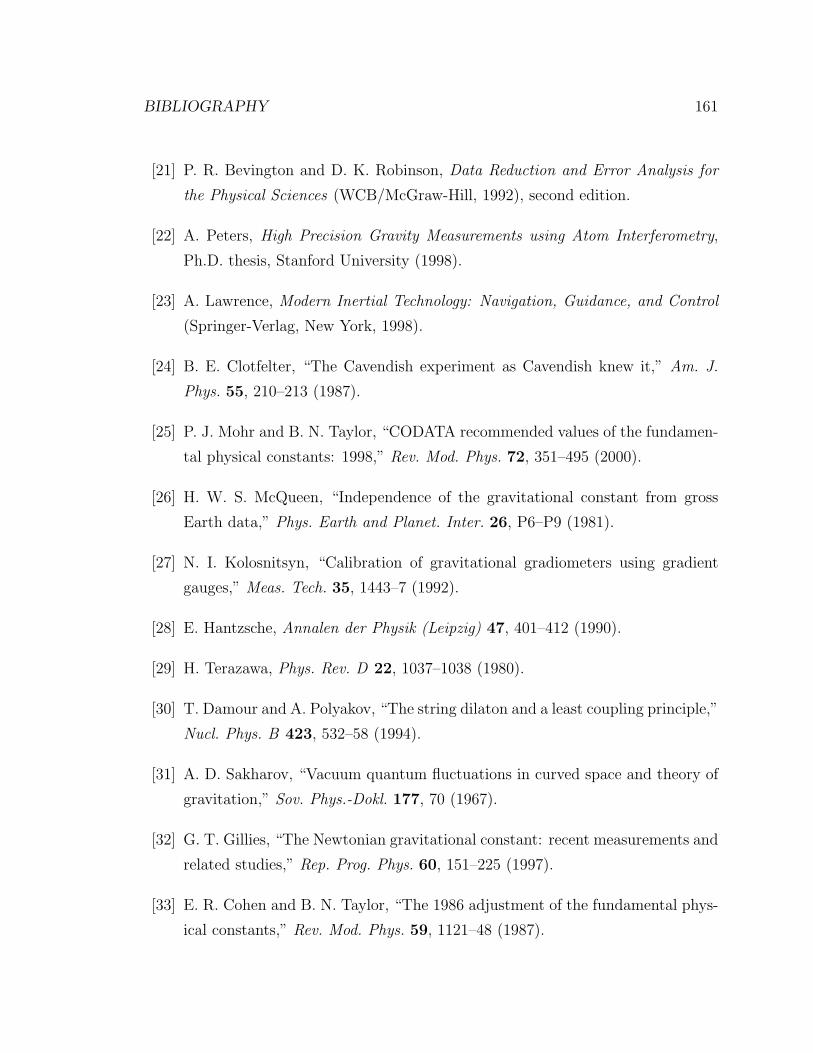
BIBLIOGRAPHY 161
[21] P. R. Bevington and D. K. Robinson, Data Reduction and Error Analysis for
the Physical Sciences (WCB/McGraw-Hill, 1992), second edition.
[22] A. Peters, High Precision Gravity Measurements using Atom Interferometry,
Ph.D. thesis, Stanford University (1998).
[23] A. Lawrence, Modern Inertial Technology: Navigation, Guidance, and Control
(Springer-Verlag, New York, 1998).
[24] B. E. Clotfelter, “The Cavendish experiment as Cavendish knew it,” Am. J.
Phys. 55, 210–213 (1987).
[25] P. J. Mohr and B. N. Taylor, “CODATA recommended values of the fundamen-
tal physical constants: 1998,” Rev. Mod. Phys. 72, 351–495 (2000).
[26] H. W. S. McQueen, “Independence of the gravitational constant from gross
Earth data,” Phys. Earth and Planet. Inter. 26, P6–P9 (1981).
[27] N. I. Kolosnitsyn, “Calibration of gravitational gradiometers using gradient
gauges,” Meas. Tech. 35, 1443–7 (1992).
[28] E. Hantzsche, Annalen der Physik (Leipzig) 47, 401–412 (1990).
[29] H. Terazawa, Phys. Rev. D 22, 1037–1038 (1980).
[30] T. Damour and A. Polyakov, “The string dilaton and a least coupling principle,”
Nucl. Phys. B 423, 532–58 (1994).
[31] A. D. Sakharov, “Vacuum quantum fluctuations in curved space and theory of
gravitation,” Sov. Phys.-Dokl. 177, 70 (1967).
[32] G. T. Gillies, “The Newtonian gravitational constant: recent measurements and
related studies,” Rep. Prog. Phys. 60, 151–225 (1997).
[33] E. R. Cohen and B. N. Taylor, “The 1986 adjustment of the fundamental phys-
ical constants,” Rev. Mod. Phys. 59, 1121–48 (1987).
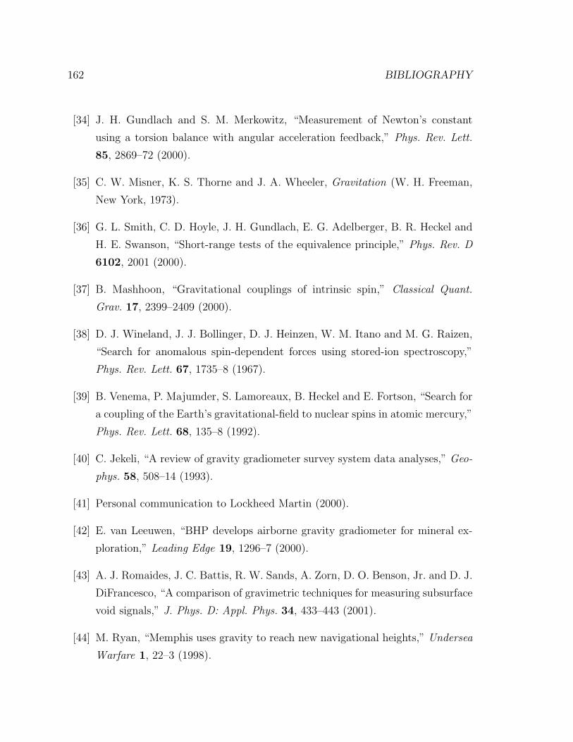
162 BIBLIOGRAPHY
[34] J. H. Gundlach and S. M. Merkowitz, “Measurement of Newton’s constant
using a torsion balance with angular acceleration feedback,” Phys. Rev. Lett.
85, 2869–72 (2000).
[35] C. W. Misner, K. S. Thorne and J. A. Wheeler, Gravitation (W. H. Freeman,
New York, 1973).
[36] G. L. Smith, C. D. Hoyle, J. H. Gundlach, E. G. Adelberger, B. R. Heckel and
H. E. Swanson, “Short-range tests of the equivalence principle,” Phys. Rev. D
6102, 2001 (2000).
[37] B. Mashhoon, “Gravitational couplings of intrinsic spin,” Classical Quant.
Grav. 17, 2399–2409 (2000).
[38] D. J. Wineland, J. J. Bollinger, D. J. Heinzen, W. M. Itano and M. G. Raizen,
“Search for anomalous spin-dependent forces using stored-ion spectroscopy,”
Phys. Rev. Lett. 67, 1735–8 (1967).
[39] B. Venema, P. Majumder, S. Lamoreaux, B. Heckel and E. Fortson, “Search for
a coupling of the Earth’s gravitational-field to nuclear spins in atomic mercury,”
Phys. Rev. Lett. 68, 135–8 (1992).
[40] C. Jekeli, “A review of gravity gradiometer survey system data analyses,” Geo-
phys. 58, 508–14 (1993).
[41] Personal communication to Lockheed Martin (2000).
[42] E. van Leeuwen, “BHP develops airborne gravity gradiometer for mineral ex-
ploration,” Leading Edge 19, 1296–7 (2000).
[43] A. J. Romaides, J. C. Battis, R. W. Sands, A. Zorn, D. O. Benson, Jr. and D. J.
DiFrancesco, “A comparison of gravimetric techniques for measuring subsurface
void signals,” J. Phys. D: Appl. Phys. 34, 433–443 (2001).
[44] M. Ryan, “Memphis uses gravity to reach new navigational heights,” Undersea
Warfare 1, 22–3 (1998).
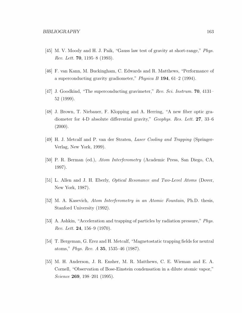
BIBLIOGRAPHY 163
[45] M. V. Moody and H. J. Paik, “Gauss law test of gravity at short-range,” Phys.
Rev. Lett. 70, 1195–8 (1993).
[46] F. van Kann, M. Buckingham, C. Edwards and R. Matthews, “Performance of
a superconducting gravity gradiometer,” Physica B 194, 61–2 (1994).
[47] J. Goodkind, “The superconducting gravimeter,” Rev. Sci. Instrum. 70, 4131–
52 (1999).
[48] J. Brown, T. Niebauer, F. Klopping and A. Herring, “A new fiber optic gra-
diometer for 4-D absolute differential gravity,” Geophys. Res. Lett. 27, 33–6
(2000).
[49] H. J. Metcalf and P. van der Straten, Laser Cooling and Trapping (Springer-
Verlag, New York, 1999).
[50] P. R. Berman (ed.), Atom Interferometry (Academic Press, San Diego, CA,
1997).
[51] L. Allen and J. H. Eberly, Optical Resonance and Two-Level Atoms (Dover,
New York, 1987).
[52] M. A. Kasevich, Atom Interferometry in an Atomic Fountain, Ph.D. thesis,
Stanford University (1992).
[53] A. Ashkin, “Acceleration and trapping of particles by radiation pressure,” Phys.
Rev. Lett. 24, 156–9 (1970).
[54] T. Bergeman, G. Erez and H. Metcalf, “Magnetostatic trapping fields for neutral
atoms,” Phys. Rev. A 35, 1535–46 (1987).
[55] M. H. Anderson, J. R. Ensher, M. R. Matthews, C. E. Wieman and E. A.
Cornell, “Observation of Bose-Einstein condensation in a dilute atomic vapor,”
Science 269, 198–201 (1995).

164 BIBLIOGRAPHY
[56] P. D. Lett, R. N. Watts, C. I. Westbrook, W. D. Phillips, P. L. Gould and H. J.
Metcalf, “Observation of atoms laser cooled below the Doppler limit,” Phys.
Rev. Lett. 61, 169–72 (1988).
[57] J. Dalibard and C. Cohen-Tannoudji, “Laser cooling below the Doppler limit
by polarization gradients: Simple theoretical models,” J. Opt. Soc. Am. B 6,
2023–45 (1989).
[58] P. J. Ungar, D. S. Weiss, E. Riis and S. Chu, “Optical molasses and multilevel
atoms: Theory,” J. Opt. Soc. Am. B 6, 2058–71 (1989).
[59] W. Wing, “On neutral particle trapping in quasistatic electromagnetic fields,”
Prog. Quant. Elect. 8, 181–99 (1984).
[60] K. E. Gibble, S. Kasapi and S. Chu, “Improved magnetooptic trapping in a
vapor cell,” Opt. Lett. 17, 526–8 (1992).
[61] M. A. Kasevich, E. Riis, S. Chu and R. G. Devoe, “RF spectroscopy in an
atomic fountain,” Phys. Rev. Lett. 63, 612–6 (1989).
[62] M. Kasevich, D. S. Weiss, E. Riis, K. Moler, S. Kasapi and S. Chu, “Atomic
velocity selection using stimulated Raman transitions,” Phys. Rev. Lett. 66,
2297–300 (1991).
[63] K. Moler, D. S. Weiss, M. Kasevich and S. Chu, “Theoretical analysis of
velocity-selective Raman transitions,” Phys. Rev. A 45, 342–8 (1992).
[64] M. Sagnac, C. R. Acad. Sci. 157, 708 (1913).
[65] H. Stolzenberg, S. Becker, G. Bollen et al., “Accurate mass determination of
short-lived isotopes by a tandem Penning-trap mass spectrometer,” Phys. Rev.
Lett. 65, 3104–7 (1990).
[66] A. L. Fetter and J. D. Walecka, Theoretical Mechanics of Particles and Continua
(Addison Wesley, 1980).
[67] H. Goldstein, Classical Mechanics (Addison Wesley, 1980), second edition.
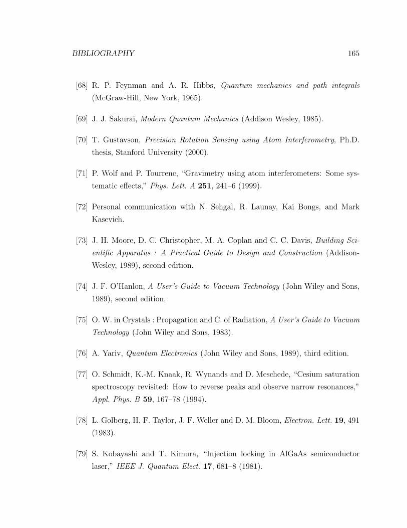
BIBLIOGRAPHY 165
[68] R. P. Feynman and A. R. Hibbs, Quantum mechanics and path integrals
(McGraw-Hill, New York, 1965).
[69] J. J. Sakurai, Modern Quantum Mechanics (Addison Wesley, 1985).
[70] T. Gustavson, Precision Rotation Sensing using Atom Interferometry, Ph.D.
thesis, Stanford University (2000).
[71] P. Wolf and P. Tourrenc, “Gravimetry using atom interferometers: Some sys-
tematic effects,” Phys. Lett. A 251, 241–6 (1999).
[72] Personal communication with N. Sehgal, R. Launay, Kai Bongs, and Mark
Kasevich.
[73] J. H. Moore, D. C. Christopher, M. A. Coplan and C. C. Davis, Building Sci-
entific Apparatus : A Practical Guide to Design and Construction (Addison-
Wesley, 1989), second edition.
[74] J. F. O’Hanlon, A User’s Guide to Vacuum Technology (John Wiley and Sons,
1989), second edition.
[75] O. W. in Crystals : Propagation and C. of Radiation, A User’s Guide to Vacuum
Technology (John Wiley and Sons, 1983).
[76] A. Yariv, Quantum Electronics (John Wiley and Sons, 1989), third edition.
[77] O. Schmidt, K.-M. Knaak, R. Wynands and D. Meschede, “Cesium saturation
spectroscopy revisited: How to reverse peaks and observe narrow resonances,”
Appl. Phys. B 59, 167–78 (1994).
[78] L. Golberg, H. F. Taylor, J. F. Weller and D. M. Bloom, Electron. Lett. 19, 491
(1983).
[79] S. Kobayashi and T. Kimura, “Injection locking in AlGaAs semiconductor
laser,” IEEE J. Quantum Elect. 17, 681–8 (1981).
166 BIBLIOGRAPHY
[80] J. N. Walpole, “Semiconductor amplifiers and lasers with tapered gain regions,”
28, 623–45 (1996).
[81] A. Abragam, The Principles of Nuclear Magnetism (Oxford Univ. Press, 1961).
[82] M. H. Levitt, “Composite pulses,” Prog. NMR Spect. 18, 61–122 (1986).
[83] P. Bouyer, T. L. Gustavson, K. G. Haritos and M. A. Kasevich, “Microwave
signal generation with optical injection locking,” Opt. Lett. 21, 1502–4 (1996).
[84] G. Santarelli, P. Laurent, P. Lemonde et al., “Quantum projection noise in an
atomic fountain: a high stability cesium frequency standard,” Phys. Rev. Lett.
82, 4619–22 (1999).
[85] R. W. P. Drever, J. L. Hall, F. V. Kowalski et al., “Laser phase and frequency
stabilization using an optical-resonator,” Appl. Phys. B 31, 97–105 (1983).
[86] J. S. Shirley, “Modulation transfer processes in optical heterodyne saturation
spectroscopy,” Opt. Lett. 7, 537–9 (1982).
[87] J. J. Synder, R. K. Raj, D. Bloch and M. Ducloy, “High-sensitivity non-linear
spectroscopy using a frequency-offset pump,” Opt. Lett. 5, 163–5 (1980).
[88] D. Bloch and M. Ducloy, “Theory of saturated line shapes in phase-conjugate
emission by resonant degenerate four-wave mixing in Doppler broadened three-
level systems,” J. Opt. Soc. Am. 73, 635–46 (1983).
[89] M. A. Kramer, R. W. Boyd, L. W. Hillman and C. R. Stroud, Jr., “Propagation
of modulated optical fields through saturable-absorbing media: a general theory
of modulation spectroscopy,” Opt. Lett. 5, 163–5 (1980).
[90] B. Do, J. Cha, D. S. Elliot and S. Smith, “Degenerate phase-conjugate four-
wave mixing in a nearly Doppler-free two-level atomic medium,” Phys. Rev. A
58, 3089–98 (1998).
[91] J. M. McGuirk, G. T. Foster, J. B. Fixler and M. A. Kasevich, “Low-noise
detection of ultracold atoms,” Opt. Lett. 26, 364–6 (2001).
BIBLIOGRAPHY 167
[92] A. P. J. M. Hensley and S. Chu, “Active low frequency vibration isolation,”
Rev. Sci. Instrum. 70, 2735–41 (1999).
[93] J. M. McGuirk, G. T. Foster, J. B. Fixler, M. J. Snadden and M. A. Kasevich,
“Sensitive absolute gravity gradiometery using atom interferometry,” (2001). In
preparation.
[94] W. H. Bay (ed.), CRC Standard Mathematical Tables and Formulae (CRC
Press, Boca Raton, 1991), 29th edition.
[95] A. W. Fitzgibbon, M. Pilu and R. B. Fisher, “Direct least squares fitting of
ellipses,” IEEE Trans. on Patt. Anal. and Mach. Intell. 21, 476–80 (1999).
[96] W. M. Itano, J. C. Bollinger, J. M. Gilligan et al., “Quantum projection noise -
population fluctuations in two-level systems,” Phys. Rev. A 47, 3554–70 (1993).
[97] A. Peters, K. Y. Chung and S. Chu, “Measurement of gravitational acceleration
by dropping atoms,” Nature 400, 849–52 (1999).
[98] Y. Tamura, Bulletin d’Informations Marees Terrestres 99, 6813 (1987).
[99] D. W. Allan, N. Ashby and C. C. Hodge, “The science of timekeeping,” Appli-
cation Note 1289, Hewlett-Packard (1997).
[100] J. M. McGuirk, M. J. Snadden and M. A. Kasevich, “Large area light-pulse
atom interferometry,” Phys. Rev. Lett. 85, 4498–501 (2000).
[101] B. Young, M. Kasevich and S. Chu, “Precision atom interferometry with light
pulses,” in Berman [50], pp. 363–406.
[102] C. J. Borde, “Matter-wave interferometers: A synthetic approach,” in Berman
[50], pp. 257–92.
[103] D. M. Giltner, R. W. McGowan and S. A. Lee, “Atom interferometer based
on Bragg scattering from standing light waves,” Phys. Rev. Lett. 75, 2638–41
(1995).
168 BIBLIOGRAPHY
[104] I. Bloch, T. W. Hansch and T. Esslinger, “Atom laser with a cw output coupler,”
Phys. Rev. Lett. 82, 3008–11 (1999).
[105] S. B. Cahn, A. Kumarakrishnan, U. Shim, T. Sleator, P. R. Berman and B. Du-
betsky, “Time-domain de Broglie wave interferometry,” Phys. Rev. Lett. 79,
784–7 (1997).
[106] P. D. Featonby, G. S. Summy, C. L. Webb et al., “Separated-path Ramsey atom
interferometer,” Phys. Rev. Lett. 81, 495–9 (1998).
[107] B. P. Anderson and M. A. Kasevich, “Macroscopic quantum interference from
atomic tunnel arrays,” Science 282, 1686–9 (1998).
[108] D. L. Haycock, S. E. Hamann, G. Klose and P. S. Jessen, “Atom trapping in
deeply bound states of a far-off-resonance optical lattice,” Phys. Rev. A 55,
R3991–4 (1998).
[109] A. J. Kerman, V. Vuletic, C. Chen and S. Chu, “Beyond optical molasses: 3D
Raman sideband cooling of atomic cesium to high phase-space density,” Phys.
Rev. Lett. 83, 439–42 (2000).
[110] P. Treutlein, K. Y. Chung and S. Chu, “High-brightness atom source for atomic
fountains,” Phys. Rev. A 63 (2001).
[111] R. Holzwarth, T. Udem, T. W. Hansch, J. C. Knight, W. J. Wadsworth and
P. S. J. Russel, “Optical frequency sythesizer for precision spectroscopy,” Opt.
Lett. 5, 163–5 (1980).


![Airborne Gravity Gradiometry in the Search for Mineral Deposits … · Airborne Gravity Gradiometry in the Search for Mineral Deposits Dransfield, M. [1] _____ 1. BHP Billiton ABSTRACT](https://img.pdfslide.us/doc/110x75/5c7950e809d3f2c9458c185e/airborne-gravity-gradiometry-in-the-search-for-mineral-deposits-airborne-gravity.jpg)


![Airborne Gravity Gradiometry in the Search for Mineral Deposits · 2015-12-14 · Airborne Gravity Gradiometry in the Search for Mineral Deposits Dransfield, M. [1] 1. BHP Billiton](https://img.pdfslide.us/doc/110x75/5e9ffa54bed7367cd454cf0a/airborne-gravity-gradiometry-in-the-search-for-mineral-deposits-2015-12-14-airborne.jpg)