Embed Size (px)
Citation preview
a project by
M.Bussieck (GAMS), F. Fiand (GAMS)
October 2017
2017 INFORMS Annual Meeting – Houston, Texas October 22-25
High Performance Computing with GAMS
2
• Motivation & Project Overview
• Parallel Interior Point Solver PIPS-IPM
• GAMS/PIPS-IPM Solver Link
– Model Annotation
– Distributed Model Generation
• Computational Experiments
• Summary & Outlook
Outline

Motivation
4
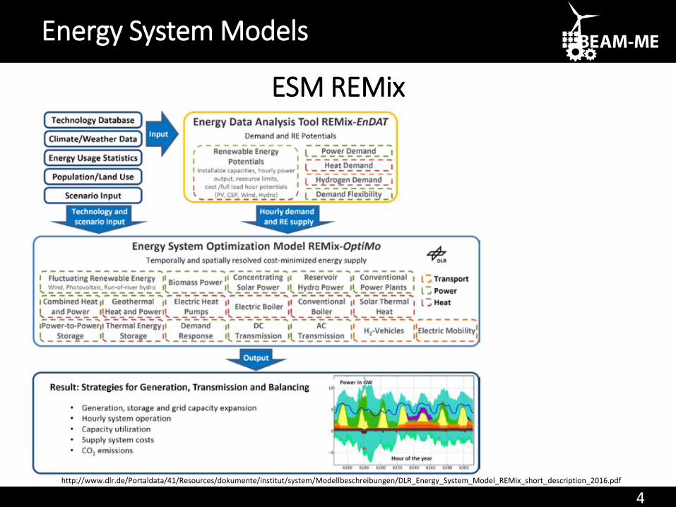
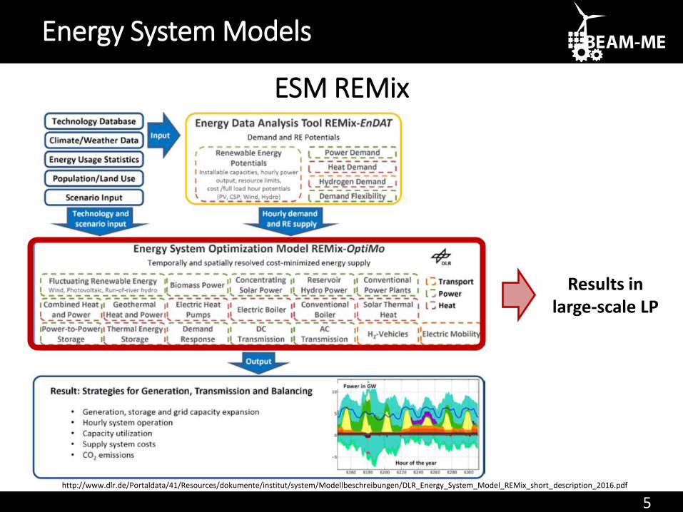
ESM REMix
Energy System Models
http://www.dlr.de/Portaldata/41/Resources/dokumente/institut/system/Modellbeschreibungen/DLR_Energy_System_Model_REMix_short_description_2016.pdf
5
ESM REMix
Energy System Models
http://www.dlr.de/Portaldata/41/Resources/dokumente/institut/system/Modellbeschreibungen/DLR_Energy_System_Model_REMix_short_description_2016.pdf
Results in large-scale LP
6
• Energy system models (ESM) have to increase in complexity to provide valuable quantitative insights for policy makers and industry:
– Uncertainty
– Large shares of renewable energies
– Complex underlying electricity systems
• Challenge:
– Increasing complexity makes solving ESM more and more difficult
Need for new solution approaches
Motivation
7
• Energy system models (ESM) have to increase in complexity to provide valuable quantitative insights for policy makers and industry:
– Uncertainty
– Large shares of renewable energies
– Complex underlying electricity systems
• Challenge:
– Increasing complexity makes solving ESM more and more difficult
Need for new solution approaches
Motivation
8
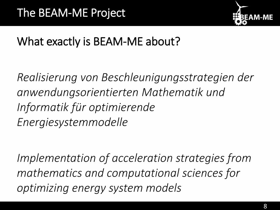
What exactly is BEAM-ME about?
Realisierung von Beschleunigungsstrategien der anwendungsorientierten Mathematik und Informatik für optimierendeEnergiesystemmodelle
Implementation of acceleration strategies from mathematics and computational sciences for optimizing energy system models
The BEAM-ME Project
9
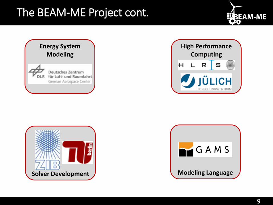
The BEAM-ME Project cont.
Energy System Modeling
Modeling Language
High Performance Computing
Solver Development
Parallel Interior Point Solver PIPS-IPM
11
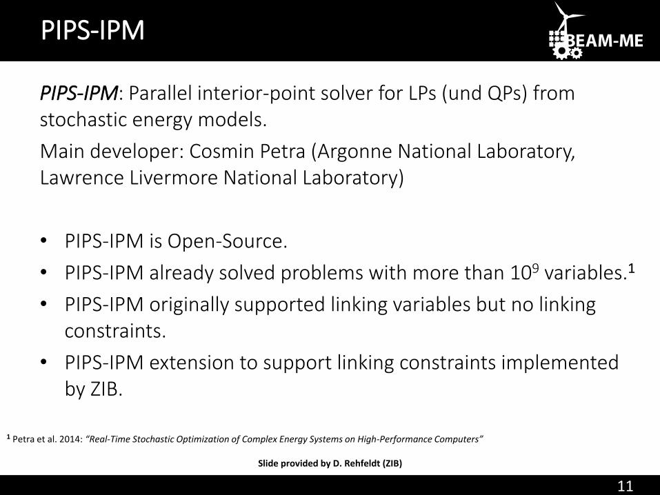
PIPS-IPM: Parallel interior-point solver for LPs (und QPs) from stochastic energy models.
Main developer: Cosmin Petra (Argonne National Laboratory, Lawrence Livermore National Laboratory)
• PIPS-IPM is Open-Source.
• PIPS-IPM already solved problems with more than 109 variables.1
• PIPS-IPM originally supported linking variables but no linking constraints.
• PIPS-IPM extension to support linking constraints implemented by ZIB.
PIPS-IPM
1 Petra et al. 2014: “Real-Time Stochastic Optimization of Complex Energy Systems on High-Performance Computers”
Slide provided by D. Rehfeldt (ZIB)
12
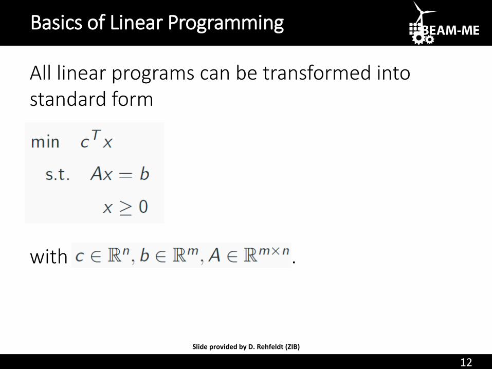
All linear programs can be transformed into standard form
with .
Basics of Linear Programming
Slide provided by D. Rehfeldt (ZIB)
13
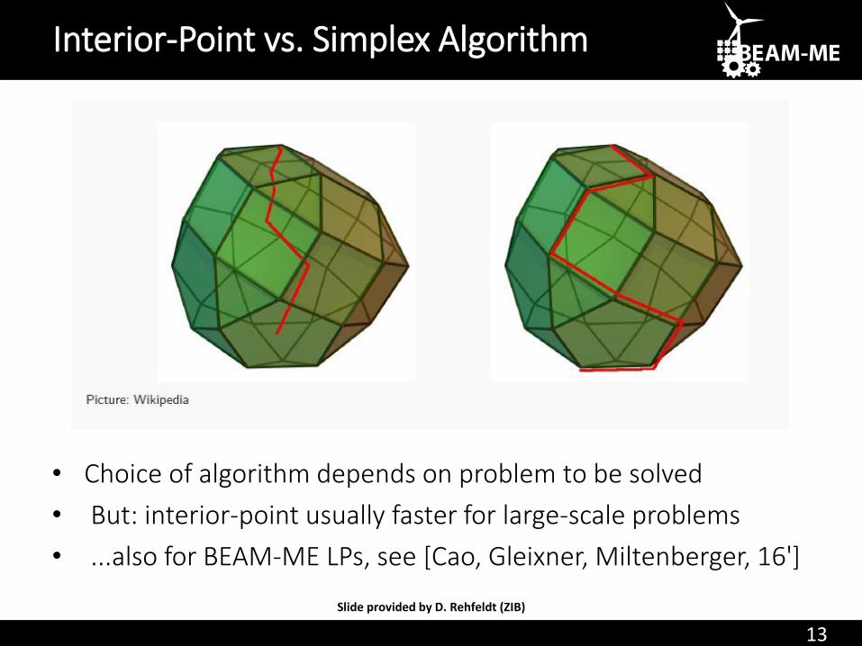
Interior-Point vs. Simplex Algorithm
• Choice of algorithm depends on problem to be solved
• But: interior-point usually faster for large-scale problems
• ...also for BEAM-ME LPs, see [Cao, Gleixner, Miltenberger, 16']
Slide provided by D. Rehfeldt (ZIB)
14
Primal Dual Interior Point Method cont.
Slide provided by D. Rehfeldt (ZIB)
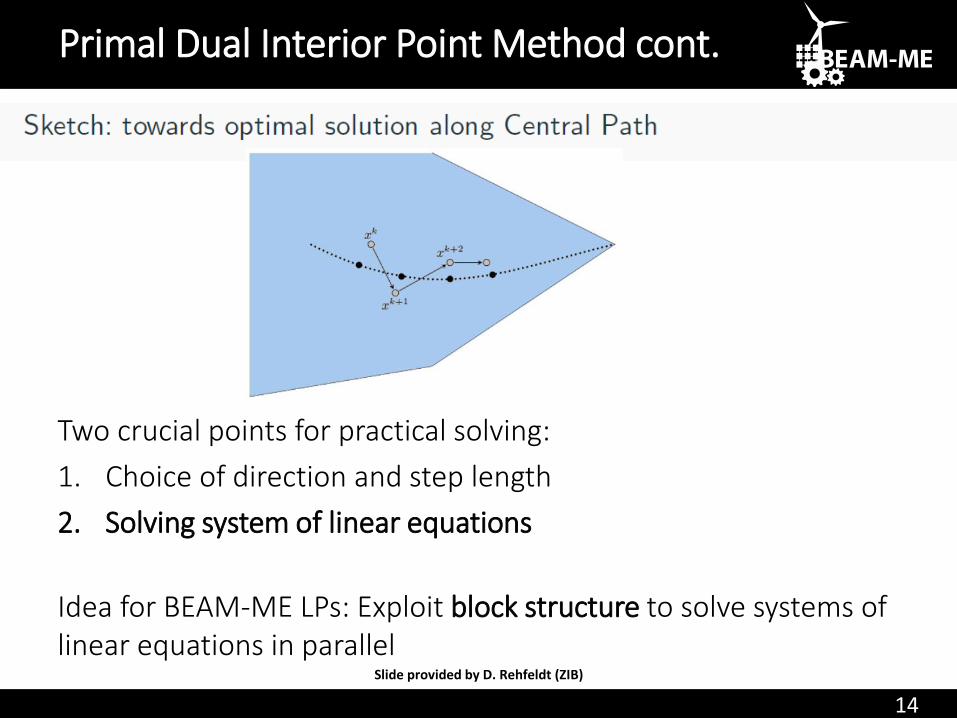
Two crucial points for practical solving:
1. Choice of direction and step length
2. Solving system of linear equations
Idea for BEAM-ME LPs: Exploit block structure to solve systems of linear equations in parallel
15
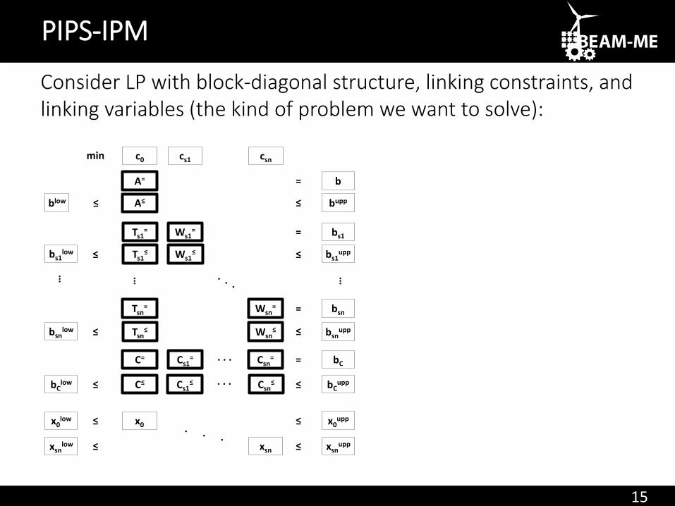
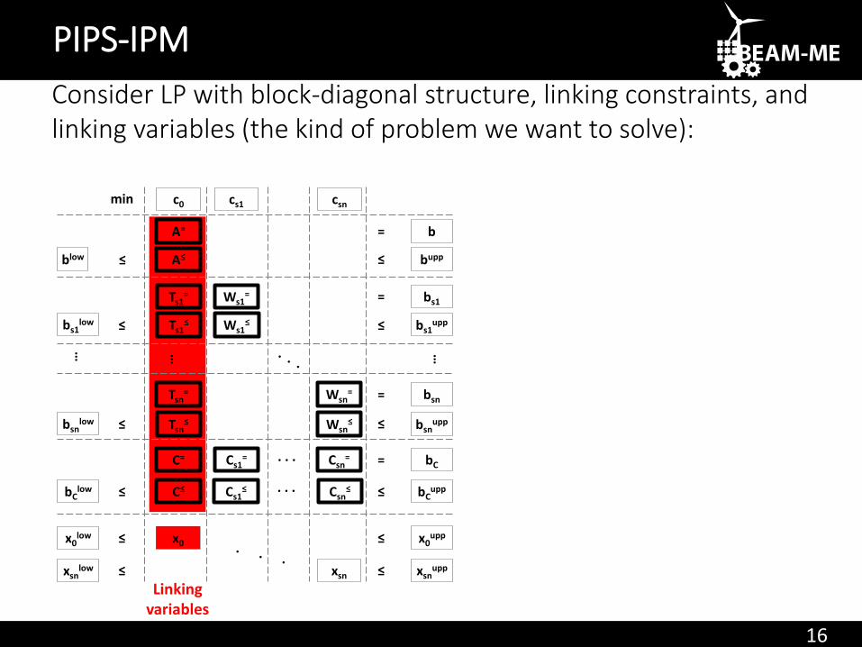
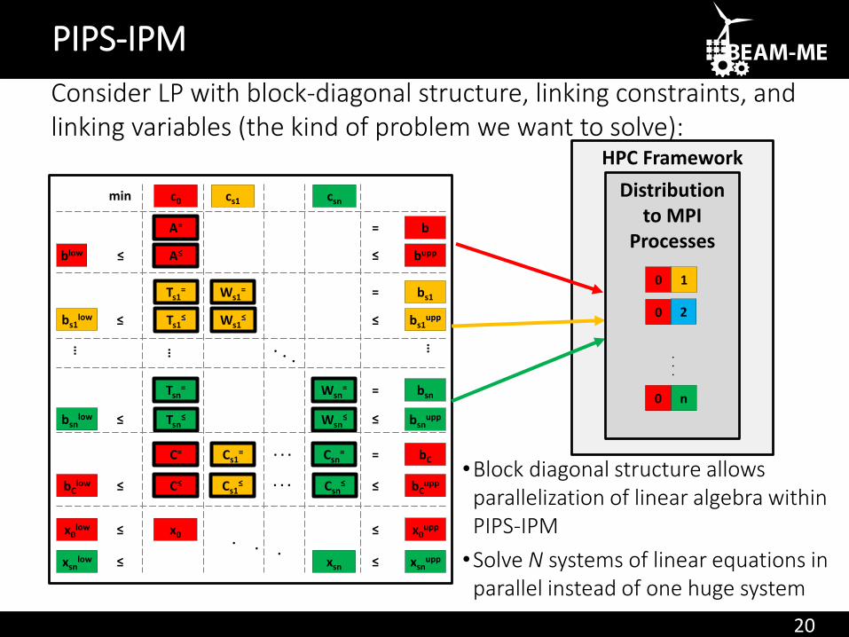
Consider LP with block-diagonal structure, linking constraints, and linking variables (the kind of problem we want to solve):
PIPS-IPM
A= b
buppA≤blow ≤ ≤
=
Ts1= Ws1
= bs1=
Tsn= Wsn
= bsn=
… …
c0 cs1 csn
Tsn≤ Wsn
≤ bsnuppbsn
low ≤ ≤
Ts1≤ Ws1
≤ bs1uppbs1
low ≤ ≤
C= Csn= = bCCs1
= . . .
C≤ Csn≤ ≤≤ bC
uppbClow Cs1
≤ . . .
min
x0 ≤≤x0low x0
upp
xsn ≤≤xsnlow xsn
upp
…
16
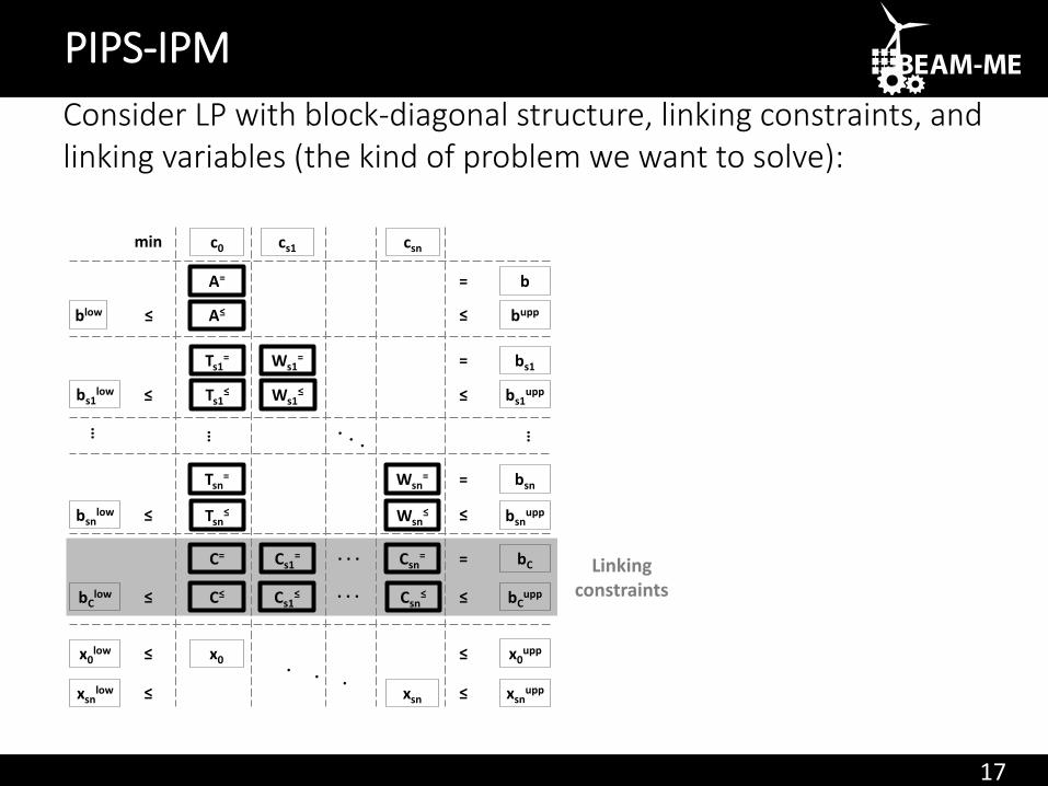
Consider LP with block-diagonal structure, linking constraints, and linking variables (the kind of problem we want to solve):
PIPS-IPM
A= b
buppA≤blow ≤ ≤
=
Ts1= Ws1
= bs1=
Tsn= Wsn
= bsn=
… …
c0 cs1 csn
Tsn≤ Wsn
≤ bsnuppbsn
low ≤ ≤
Ts1≤ Ws1
≤ bs1uppbs1
low ≤ ≤
C= Csn= = bCCs1
= . . .
C≤ Csn≤ ≤≤ bC
uppbClow Cs1
≤ . . .
min
x0 ≤≤x0low x0
upp
xsn ≤≤xsnlow xsn
upp
…
Linking variables
17
Linking constraints
Consider LP with block-diagonal structure, linking constraints, and linking variables (the kind of problem we want to solve):
PIPS-IPM
A= b
buppA≤blow ≤ ≤
=
Ts1= Ws1
= bs1=
Tsn= Wsn
= bsn=
… …
c0 cs1 csn
Tsn≤ Wsn
≤ bsnuppbsn
low ≤ ≤
Ts1≤ Ws1
≤ bs1uppbs1
low ≤ ≤
C= Csn= = bCCs1
= . . .
C≤ Csn≤ ≤≤ bC
uppbClow Cs1
≤ . . .
min
x0 ≤≤x0low x0
upp
xsn ≤≤xsnlow xsn
upp
…
18
Recourse decision blocks
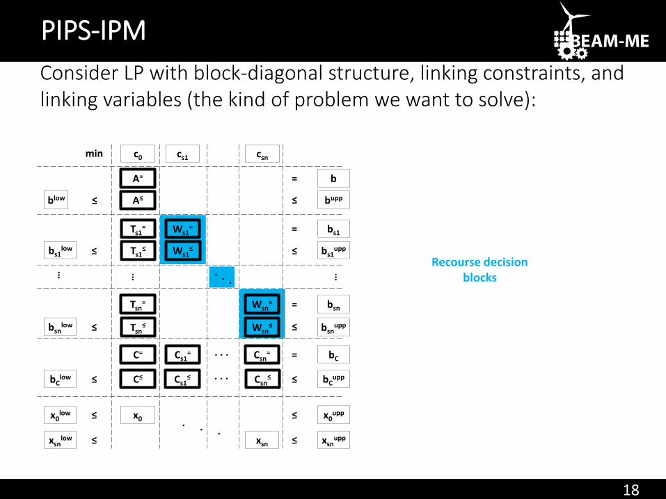
Consider LP with block-diagonal structure, linking constraints, and linking variables (the kind of problem we want to solve):
PIPS-IPM
A= b
buppA≤blow ≤ ≤
=
Ts1= Ws1
= bs1=
Tsn= Wsn
= bsn=
… …
c0 cs1 csn
Tsn≤ Wsn
≤ bsnuppbsn
low ≤ ≤
Ts1≤ Ws1
≤ bs1uppbs1
low ≤ ≤
C= Csn= = bCCs1
= . . .
C≤ Csn≤ ≤≤ bC
uppbClow Cs1
≤ . . .
min
x0 ≤≤x0low x0
upp
xsn ≤≤xsnlow xsn
upp
…
19
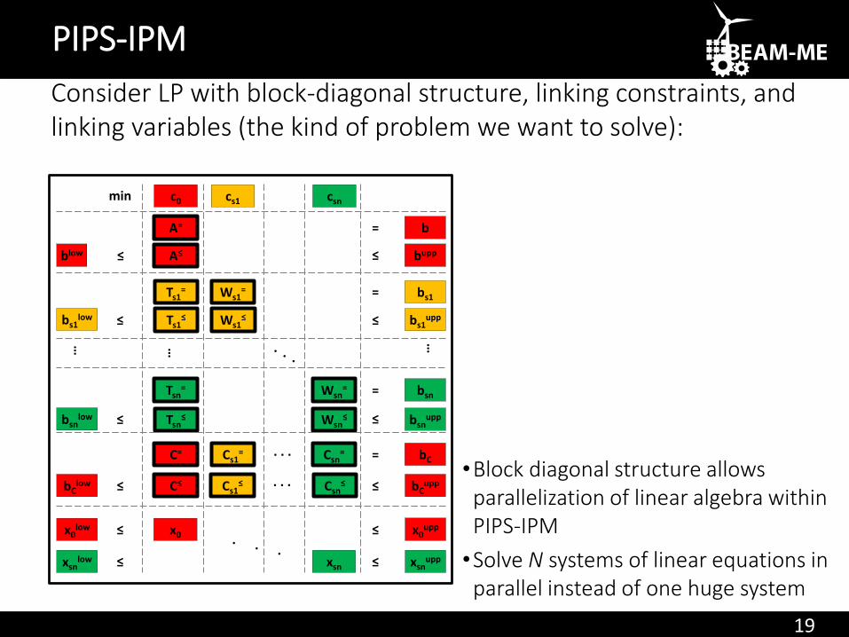
Consider LP with block-diagonal structure, linking constraints, and linking variables (the kind of problem we want to solve):
PIPS-IPM
A= b
buppA≤blow ≤ ≤
=
Ts1= Ws1
= bs1=
Tsn= Wsn
= bsn=
… …
c0 cs1 csn
Tsn≤ Wsn
≤ bsnuppbsn
low ≤ ≤
Ts1≤ Ws1
≤ bs1uppbs1
low ≤ ≤
C= Csn= = bCCs1
= . . .
C≤ Csn≤ ≤≤ bC
uppbClow Cs1
≤ . . .
min
x0 ≤≤x0low x0
upp
xsn ≤≤xsnlow xsn
upp
…
•Block diagonal structure allows parallelization of linear algebra within PIPS-IPM
•Solve N systems of linear equations in parallel instead of one huge system
20
HPC Framework
Consider LP with block-diagonal structure, linking constraints, and linking variables (the kind of problem we want to solve):
PIPS-IPM
A= b
buppA≤blow ≤ ≤
=
Ts1= Ws1
= bs1=
Tsn= Wsn
= bsn=
… …
c0 cs1 csn
Tsn≤ Wsn
≤ bsnuppbsn
low ≤ ≤
Ts1≤ Ws1
≤ bs1uppbs1
low ≤ ≤
C= Csn= = bCCs1
= . . .
C≤ Csn≤ ≤≤ bC
uppbClow Cs1
≤ . . .
min
x0 ≤≤x0low x0
upp
xsn ≤≤xsnlow xsn
upp
…
•Block diagonal structure allows parallelization of linear algebra within PIPS-IPM
•Solve N systems of linear equations in parallel instead of one huge system
Distribution to MPI
Processes
0 1
n
. . .
0 2
0

GAMS/PIPS-IPM Solver Link
Model Annotation
22
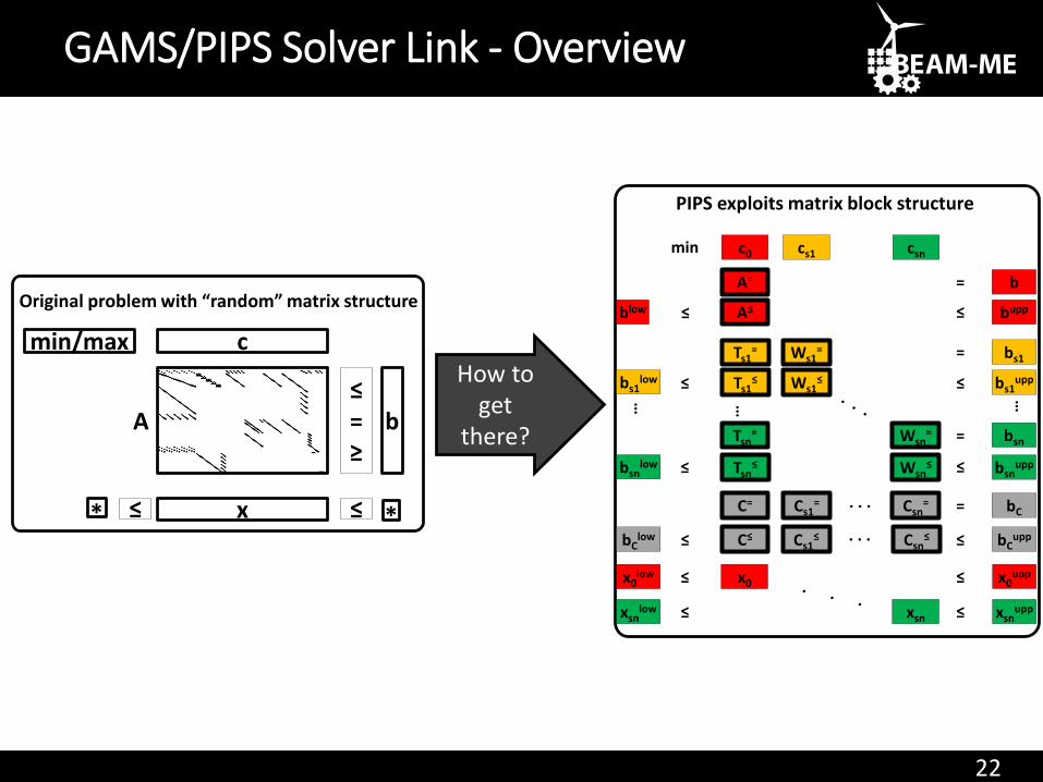
GAMS/PIPS Solver Link - Overview
How to get
there?b
≤= ≥
cmin/max
x ≤ *
A
Original problem with “random” matrix structure
≤*
PIPS exploits matrix block structure
A= b
buppA≤blow ≤ ≤
=
Ts1= Ws1
= bs1=
Tsn= Wsn
= bsn=
… …
c0 cs1 csn
Tsn≤ Wsn
≤ bsnuppbsn
low ≤ ≤
Ts1≤ Ws1
≤ bs1uppbs1
low ≤ ≤
C= Csn= = bCCs1
= . . .
C≤ Csn≤ ≤≤ bC
uppbClow Cs1
≤ . . .
min
x0 ≤≤x0low x0
upp
xsn ≤≤xsnlow xsn
upp
…
23
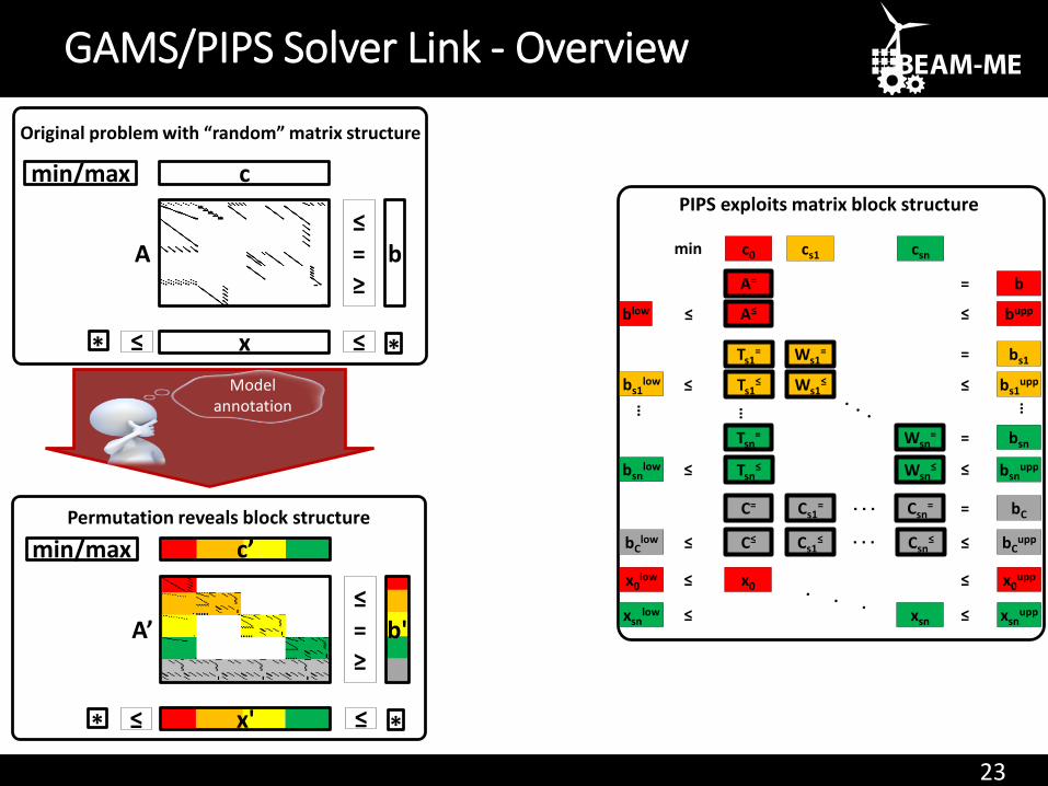
GAMS/PIPS Solver Link - Overview
b≤= ≥
cmin/max
x ≤ *
A
Original problem with “random” matrix structure
≤*
PIPS exploits matrix block structure
A= b
buppA≤blow ≤ ≤
=
Ts1= Ws1
= bs1=
Tsn= Wsn
= bsn=
… …
c0 cs1 csn
Tsn≤ Wsn
≤ bsnuppbsn
low ≤ ≤
Ts1≤ Ws1
≤ bs1uppbs1
low ≤ ≤
C= Csn= = bCCs1
= . . .
C≤ Csn≤ ≤≤ bC
uppbClow Cs1
≤ . . .
min
x0 ≤≤x0low x0
upp
xsn ≤≤xsnlow xsn
upp
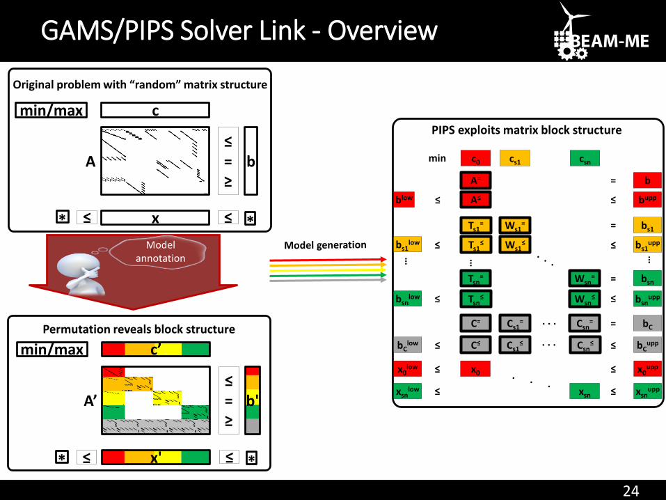
…Model
annotation
b'≤= ≥
c’min/max
x'
A’
Permutation reveals block structure
≤* ≤ *
24
GAMS/PIPS Solver Link - Overview
b≤= ≥
cmin/max
x ≤ *
A
Original problem with “random” matrix structure
≤*
PIPS exploits matrix block structure
A= b
buppA≤blow ≤ ≤
=
Ts1= Ws1
= bs1=
Tsn= Wsn
= bsn=
… …
c0 cs1 csn
Tsn≤ Wsn
≤ bsnuppbsn
low ≤ ≤
Ts1≤ Ws1
≤ bs1uppbs1
low ≤ ≤
C= Csn= = bCCs1
= . . .
C≤ Csn≤ ≤≤ bC
uppbClow Cs1
≤ . . .
min
x0 ≤≤x0low x0
upp
xsn ≤≤xsnlow xsn
upp
…Model
annotation
b'≤= ≥
c’min/max
x'
A’
Permutation reveals block structure
≤* ≤ *
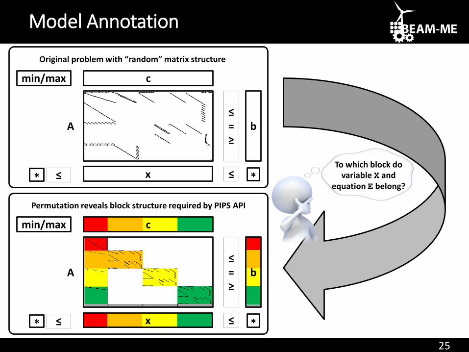
25
Model Annotation
b≤= ≥
cmin/max
x ≤ *
A
Original problem with “random” matrix structure
≤*
b≤= ≥
cmin/max
x ≤ *
A
Permutation reveals block structure required by PIPS API
≤*
To which block do variable X and
equation E belong?
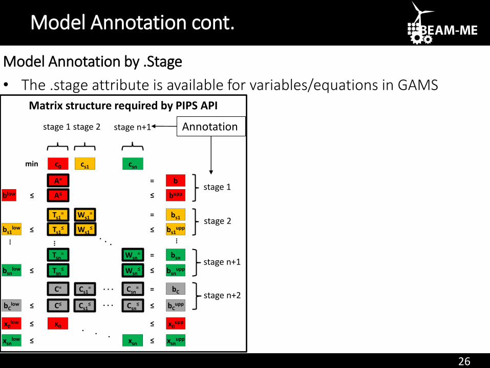
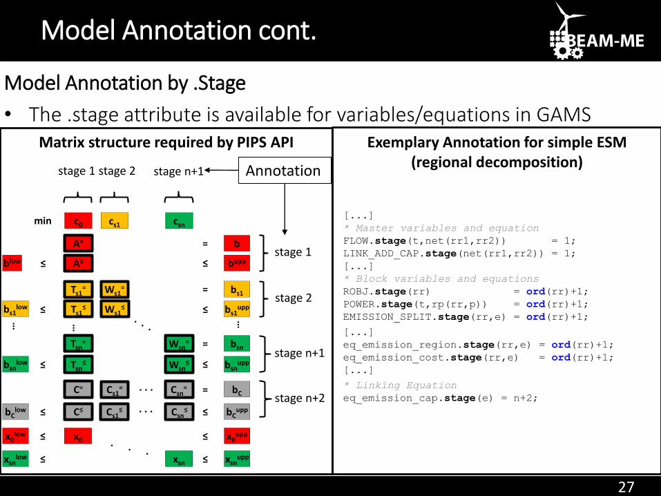
26
Model Annotation by .Stage
• The .stage attribute is available for variables/equations in GAMS
stage 1A= b
buppA≤blow ≤ ≤
=
Ts1= Ws1
= bs1=
Tsn= Wsn
= bsn=
… …
c0 cs1 csn
Tsn≤ Wsn
≤ bsnuppbsn
low ≤ ≤
Ts1≤ Ws1
≤ bs1uppbs1
low ≤ ≤
C= Csn= = bCCs1
= . . .
C≤ Csn≤ ≤≤ bC
uppbClow Cs1
≤ . . .
min
x0 ≤≤x0low x0
upp
xsn ≤≤xsnlow xsn
upp
…
stage 2
stage n+1
stage n+2
stage 1 stage 2 stage n+1
Matrix structure required by PIPS API
Annotation
Model Annotation cont.
27
Model Annotation by .Stage
• The .stage attribute is available for variables/equations in GAMS
stage 1A= b
buppA≤blow ≤ ≤
=
Ts1= Ws1
= bs1=
Tsn= Wsn
= bsn=
… …
c0 cs1 csn
Tsn≤ Wsn
≤ bsnuppbsn
low ≤ ≤
Ts1≤ Ws1
≤ bs1uppbs1
low ≤ ≤
C= Csn= = bCCs1
= . . .
C≤ Csn≤ ≤≤ bC
uppbClow Cs1
≤ . . .
min
x0 ≤≤x0low x0
upp
xsn ≤≤xsnlow xsn
upp
…
stage 2
stage n+1
stage n+2
stage 1 stage 2 stage n+1
Matrix structure required by PIPS API
Annotation
Exemplary Annotation for simple ESM(regional decomposition)
[...]
* Master variables and equation
FLOW.stage(t,net(rr1,rr2)) = 1;
LINK_ADD_CAP.stage(net(rr1,rr2)) = 1;
[...]
* Block variables and equations
ROBJ.stage(rr) = ord(rr)+1;
POWER.stage(t,rp(rr,p)) = ord(rr)+1;
EMISSION_SPLIT.stage(rr,e) = ord(rr)+1;
[...]
eq_emission_region.stage(rr,e) = ord(rr)+1;
eq_emission_cost.stage(rr,e) = ord(rr)+1;
[...]
* Linking Equation
eq_emission_cap.stage(e) = n+2;
Model Annotation cont.
28
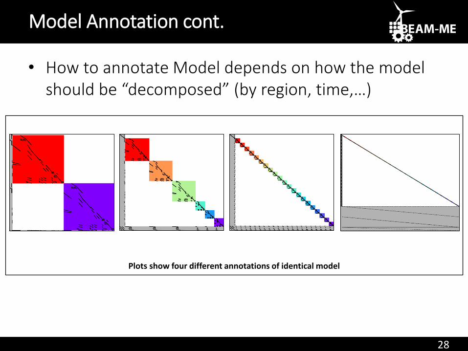
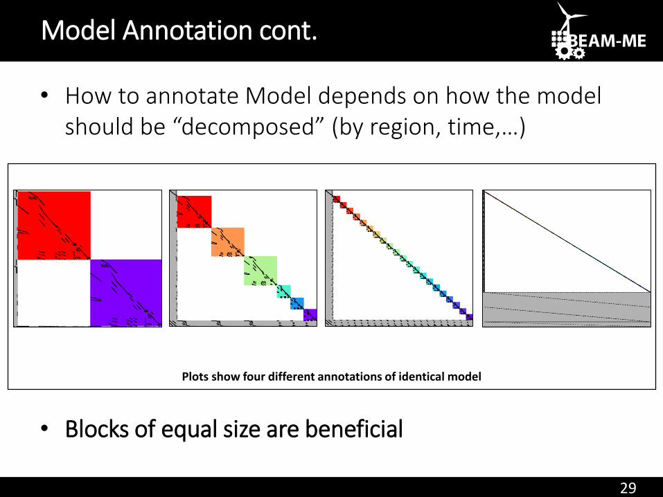
• How to annotate Model depends on how the model should be “decomposed” (by region, time,…)
Model Annotation cont.
Plots show four different annotations of identical model
29
• How to annotate Model depends on how the model should be “decomposed” (by region, time,…)
• Blocks of equal size are beneficial
Model Annotation cont.
Plots show four different annotations of identical model
GAMS/PIPS Solver Link
Distributed Model Generation
31
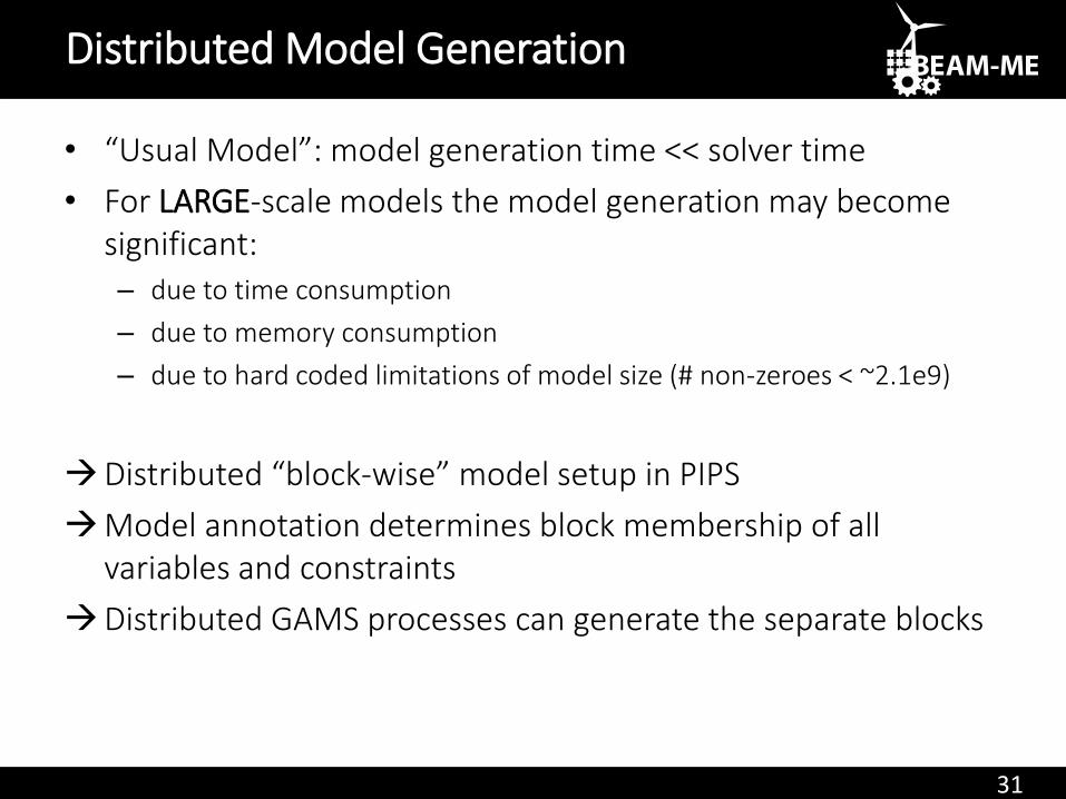
• “Usual Model”: model generation time << solver time
• For LARGE-scale models the model generation may become significant:– due to time consumption
– due to memory consumption
– due to hard coded limitations of model size (# non-zeroes < ~2.1e9)
Distributed “block-wise” model setup in PIPS
Model annotation determines block membership of all variables and constraints
Distributed GAMS processes can generate the separate blocks
Distributed Model Generation
32
Distributed Model Generation cont.
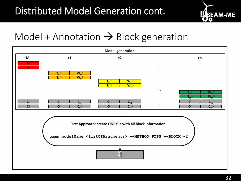
Model + Annotation Block generationModel generation
A=
A≤
C=
C≤
Ts1= Ws1
=
Ts1≤ Ws1
≤
C= Cs1=
C≤ Cs1≤
Ts2= Ws2
=
Ts2≤ Ws2
≤
C= Cs2=
C≤ Cs2≤
Tsn= Wsn
=
Tsn≤ Wsn
≤
C= Csn=
C≤ Csn≤
. . .
. . .
M r1 r2 rn
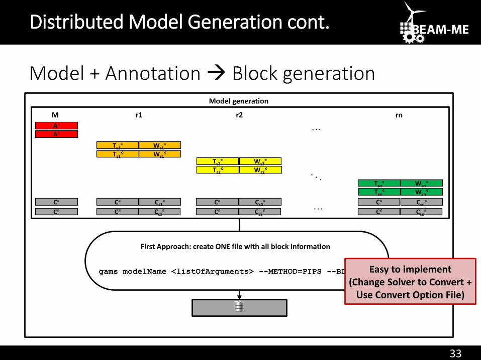
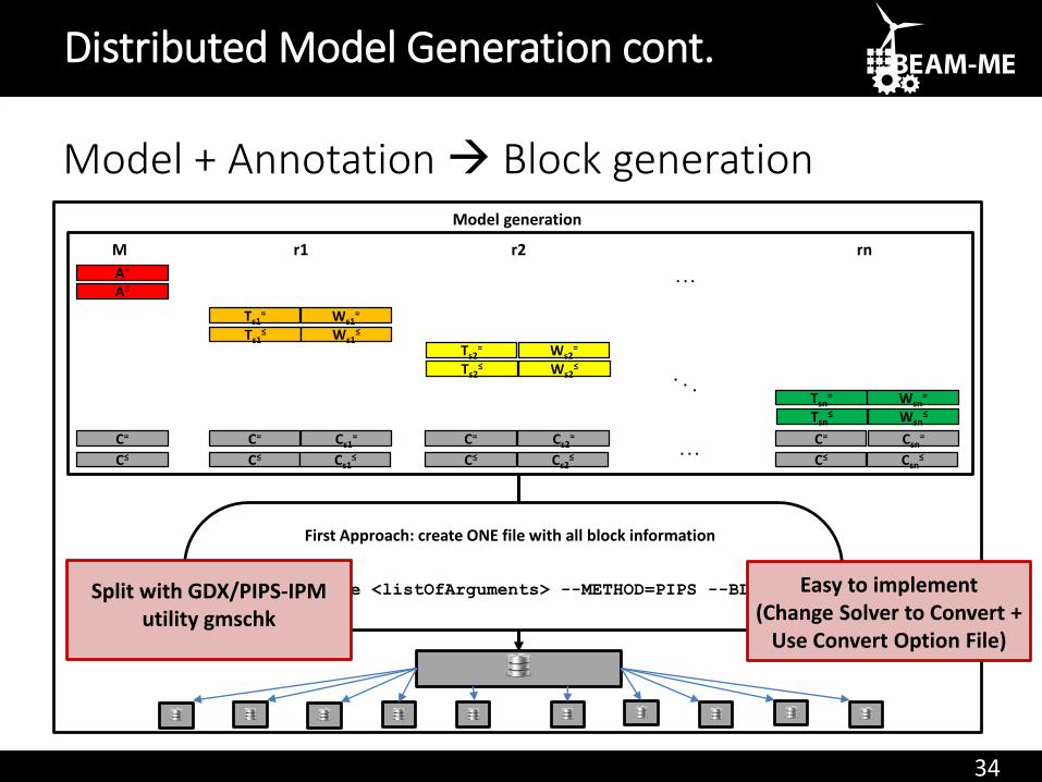
gams modelName <listOfArguments> --METHOD=PIPS --BLOCK=-2
First Approach: create ONE file with all block information
33
Distributed Model Generation cont.
Model + Annotation Block generationModel generation
A=
A≤
C=
C≤
Ts1= Ws1
=
Ts1≤ Ws1
≤
C= Cs1=
C≤ Cs1≤
Ts2= Ws2
=
Ts2≤ Ws2
≤
C= Cs2=
C≤ Cs2≤
Tsn= Wsn
=
Tsn≤ Wsn
≤
C= Csn=
C≤ Csn≤
. . .
. . .
M r1 r2 rn
gams modelName <listOfArguments> --METHOD=PIPS --BLOCK=-2
First Approach: create ONE file with all block information
Easy to implement (Change Solver to Convert +
Use Convert Option File)
34
Distributed Model Generation cont.
Model + Annotation Block generationModel generation
A=
A≤
C=
C≤
Ts1= Ws1
=
Ts1≤ Ws1
≤
C= Cs1=
C≤ Cs1≤
Ts2= Ws2
=
Ts2≤ Ws2
≤
C= Cs2=
C≤ Cs2≤
Tsn= Wsn
=
Tsn≤ Wsn
≤
C= Csn=
C≤ Csn≤
. . .
. . .
M r1 r2 rn
gams modelName <listOfArguments> --METHOD=PIPS --BLOCK=-2
First Approach: create ONE file with all block information
Easy to implement (Change Solver to Convert +
Use Convert Option File)
Split with GDX/PIPS-IPM utility gmschk
35
Distributed Model Generation cont.
Model + Annotation Block generationModel generation
A=
A≤
C=
C≤
Ts1= Ws1
=
Ts1≤ Ws1
≤
C= Cs1=
C≤ Cs1≤
Ts2= Ws2
=
Ts2≤ Ws2
≤
C= Cs2=
C≤ Cs2≤
Tsn= Wsn
=
Tsn≤ Wsn
≤
C= Csn=
C≤ Csn≤
. . .
. . .
M r1 r2 rn
. . .
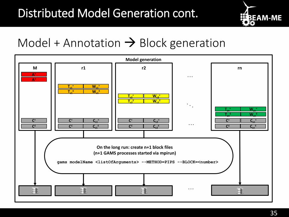
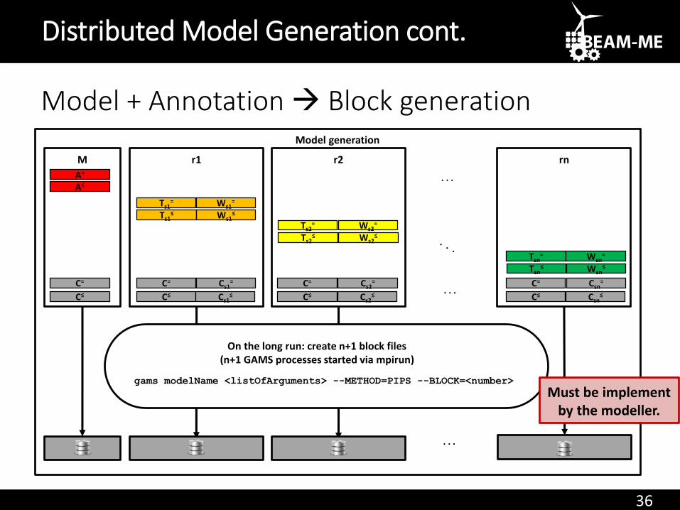
gams modelName <listOfArguments> --METHOD=PIPS --BLOCK=<number>
On the long run: create n+1 block files (n+1 GAMS processes started via mpirun)
36
Distributed Model Generation cont.
Model + Annotation Block generationModel generation
A=
A≤
C=
C≤
Ts1= Ws1
=
Ts1≤ Ws1
≤
C= Cs1=
C≤ Cs1≤
Ts2= Ws2
=
Ts2≤ Ws2
≤
C= Cs2=
C≤ Cs2≤
Tsn= Wsn
=
Tsn≤ Wsn
≤
C= Csn=
C≤ Csn≤
. . .
. . .
M r1 r2 rn
. . .
gams modelName <listOfArguments> --METHOD=PIPS --BLOCK=<number>
On the long run: create n+1 block files (n+1 GAMS processes started via mpirun)
Must be implement by the modeller.
Computational Experiments
38
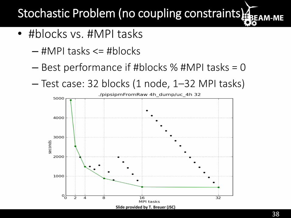
• #blocks vs. #MPI tasks
– #MPI tasks <= #blocks
– Best performance if #blocks % #MPI tasks = 0
– Test case: 32 blocks (1 node, 1–32 MPI tasks)
Stochastic Problem (no coupling constraints)
Slide provided by T. Breuer (JSC)
39
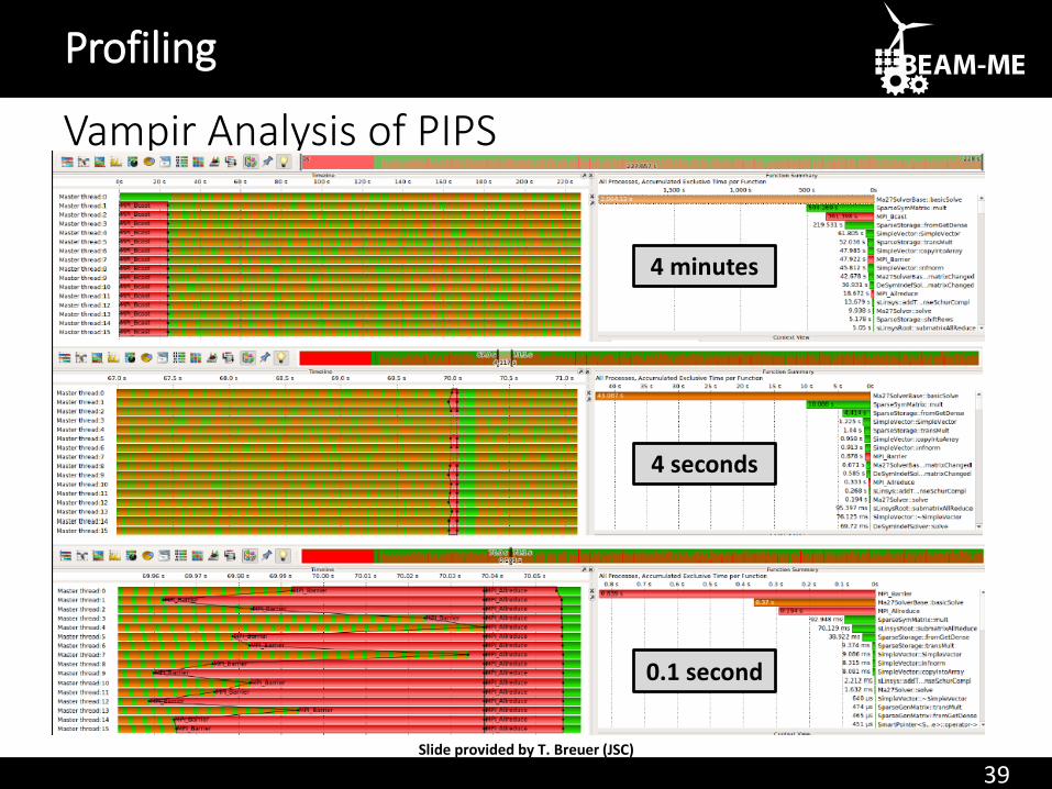
Vampir Analysis of PIPS
Profiling
Slide provided by T. Breuer (JSC)
4 minutes
4 seconds
0.1 second
40
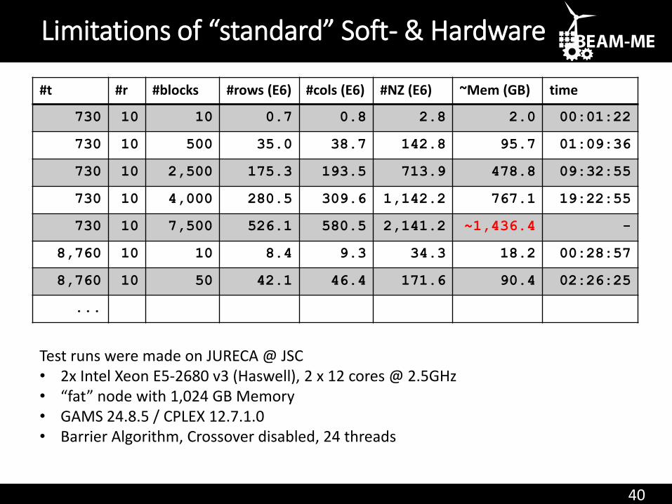
Limitations of “standard” Soft- & Hardware
#t #r #blocks #rows (E6) #cols (E6) #NZ (E6) ~Mem (GB) time
730 10 10 0.7 0.8 2.8 2.0 00:01:22
730 10 500 35.0 38.7 142.8 95.7 01:09:36
730 10 2,500 175.3 193.5 713.9 478.8 09:32:55
730 10 4,000 280.5 309.6 1,142.2 767.1 19:22:55
730 10 7,500 526.1 580.5 2,141.2 ~1,436.4 -
8,760 10 10 8.4 9.3 34.3 18.2 00:28:57
8,760 10 50 42.1 46.4 171.6 90.4 02:26:25
...
Test runs were made on JURECA @ JSC• 2x Intel Xeon E5-2680 v3 (Haswell), 2 x 12 cores @ 2.5GHz• “fat” node with 1,024 GB Memory• GAMS 24.8.5 / CPLEX 12.7.1.0• Barrier Algorithm, Crossover disabled, 24 threads

Summary & Outlook
42
• PIPS-IPM
– Change(d) linear solver from MA27 (default) to PARDISO SC
– Improve numerical stability
– Implement (structure-preserving, parallel?) preprocessing
• GAMS/PIPS-IPM Link
– Integrate model generation and solution into one user friendly process
– Better user control of GAMS/PIPS• options (algorithmic, limits, tolerances)
• Annotation can be adapted for other Decomposition approaches (e.g. CPLEX Benders)
• GAMS-MPI/Embedded Code:
– Implementation of Benders Decomposition in GAMS for ESM using the GAMS embedded code facility with Python package mpi4py to work with MPI (see talk of L. Westermann, Tuesday, Oct 24, 10:30 - 12:00track TB74 - room 372C)
• Apply developed methods to several other large-scale ESM in Model Experiment: BALMOREL, DIMENSION, …
Summary & Outlook
43
Project BEAM-ME
a project by