High organic inputs explain shallow and deep SOC storage

Biogeosciences, 15, 297–317, 2018https://doi.org/10.5194/bg-15-297-2018© Author(s) 2018. This work is distributed underthe Creative Commons Attribution 3.0 License.

High organic inputs explain shallow and deep SOC storage ina long-term agroforestry system – combining experimentaland modeling approachesRémi Cardinael1,2,3,4, Bertrand Guenet5, Tiphaine Chevallier1, Christian Dupraz6, Thomas Cozzi2, and Claire Chenu2

1Eco&Sols, IRD, CIRAD, INRA, Montpellier SupAgro, Univ. Montpellier, Montpellier, France2AgroParisTech, UMR Ecosys, Avenue Lucien Brétignières, 78850 Thiverval-Grignon, France3CIRAD, UPR AIDA, 34398 Montpellier, France4AIDA, Univ Montpellier, CIRAD, Montpellier, France5Laboratoire des Sciences du Climat et de l’Environnement, UMR CEA-CNRS-UVSQ, CE L’Orme des Merisiers,91191 Gif-Sur-Yvette, France6System, INRA, CIRAD, Montpellier SupAgro, Univ. Montpellier, Montpellier, France

Correspondence: Rémi Cardinael ([email protected])

Received: 4 April 2017 – Discussion started: 12 April 2017Revised: 1 December 2017 – Accepted: 4 December 2017 – Published: 15 January 2018

Abstract. Agroforestry is an increasingly popular farmingsystem enabling agricultural diversification and providingseveral ecosystem services. In agroforestry systems, soil or-ganic carbon (SOC) stocks are generally increased, but it isdifficult to disentangle the different factors responsible forthis storage. Organic carbon (OC) inputs to the soil may belarger, but SOC decomposition rates may be modified ow-ing to microclimate, physical protection, or priming effectfrom roots, especially at depth. We used an 18-year-old sil-voarable system associating hybrid walnut trees (Juglans re-gia × nigra) and durum wheat (Triticum turgidum L. subsp.durum) and an adjacent agricultural control plot to quantifyall OC inputs to the soil – leaf litter, tree fine root senescence,crop residues, and tree row herbaceous vegetation – and mea-sured SOC stocks down to 2 m of depth at varying distancesfrom the trees. We then proposed a model that simulates SOCdynamics in agroforestry accounting for both the whole soilprofile and the lateral spatial heterogeneity. The model wascalibrated to the control plot only.

Measured OC inputs to soil were increased by about 40 %(+ 1.11 tCha−1 yr−1) down to 2 m of depth in the agro-forestry plot compared to the control, resulting in an addi-tional SOC stock of 6.3 tCha−1 down to 1 m of depth. How-ever, most of the SOC storage occurred in the first 30 cmof soil and in the tree rows. The model was strongly val-idated, properly describing the measured SOC stocks and

distribution with depth in agroforestry tree rows and alleys.It showed that the increased inputs of fresh biomass to soilexplained the observed additional SOC storage in the agro-forestry plot. Moreover, only a priming effect variant of themodel was able to capture the depth distribution of SOCstocks, suggesting the priming effect as a possible mecha-nism driving deep SOC dynamics. This result questions thepotential of soils to store large amounts of carbon, especiallyat depth. Deep-rooted trees modify OC inputs to soil, a pro-cess that deserves further study given its potential effects onSOC dynamics.

1 Introduction

Agroforestry systems are complex agroecosystems combin-ing trees and crops or pastures within the same field (Nair,1985, 1993; Somarriba, 1992). More precisely, silvoarablesystems associate parallel tree rows with annual crops. Somestudies showed that these systems could be very productive,with a land equivalent ratio (Mead and Willey, 1980) reach-ing up to 1.3 (Graves et al., 2007). Silvoarable systems maytherefore produce up to 30 % more marketable biomass onthe same area of land compared to crops and trees grownseparately. This performance can be explained by a better use

Published by Copernicus Publications on behalf of the European Geosciences Union.

298 R. Cardinael et al.: Modeling SOC dynamics in agroforestry

of water, nutrients, and light by the agroecosystem through-out the year. Trees grown in silvoarable systems usually growfaster than the same trees grown in forest ecosystems becauseof their lower density and because they also benefit fromcrop fertilization (Balandier and Dupraz, 1999; Chaudhryet al., 2003; Chifflot et al., 2006). In temperate regions, farm-ers usually grow one crop per year, and this association oftrees can extend the growing period on the field scale, espe-cially when winter crops are intercropped with trees havinga late bud break (Burgess et al., 2004). However, after severalyears, a decrease in crop yield can be observed in mature andhighly dense plantations, especially close to the trees, due tocompetition between crops and trees for light, water, and nu-trients (Burgess et al., 2004; Dufour et al., 2013; Yin and He,1997).

Part of the additional biomass produced in agroforestry isused for economical purposes, such as timber or fruit pro-duction. Leaves, tree fine roots, pruning residues, and theherbaceous vegetation growing in the tree rows will usuallyreturn to the soil, contributing to a higher input of organiccarbon (OC) to the soil compared to an agricultural field (Pe-ichl et al., 2006).

In such systems, the observed soil organic carbon (SOC)stocks are also generally higher compared to cropland (Al-brecht and Kandji, 2003; Kim et al., 2016; Lorenz and Lal,2014). Cardinael et al. (2017) measured a mean SOC stockaccumulation rate of 0.24 (0.09–0.46) tCha−1 yr−1 at 0–30 cm of depth in several silvoarable systems compared toagricultural plots in France. Higher SOC stocks were alsofound in Canadian agroforestry systems, but measured onlyto 20 cm of depth (Bambrick et al., 2010; Oelbermann et al.,2004; Peichl et al., 2006).

To our knowledge, we are still not able to disentangle thefactors responsible for such a higher SOC storage. This SOCstorage might be due to higher OC inputs, but it could also befavored by a modification of the SOC decomposition owingto a change in SOC physical protection (Haile et al., 2010)and/or in soil temperature and moisture.

The introduction of trees in an agricultural field modifiesthe amount, but also the distribution, of fresh organic car-bon (FOC) input to the soil both vertically and horizontally(Bambrick et al., 2010; Howlett et al., 2011; Peichl et al.,2006). FOC inputs from the trees decrease with increasingdistance from the trunk and with soil depth (Moreno et al.,2005). In contrast, crop yield usually increases with increas-ing distance from the trees (Dufour et al., 2013; Li et al.,2008). Therefore, the proportions of FOC coming from boththe crop residues and the trees change with distance from thetrees, soil depth, and time.

Tree fine roots (diameter≤ 2 mm) are the most active partof root systems (Eissenstat and Yanai, 1997) and play a majorrole in carbon cycling. In silvoarable systems, tree fine rootdistribution within the soil profile is strongly modified dueto competition with the crop, inducing a deeper rooting com-pared to trees grown in forest ecosystems (Cardinael et al.,

2015a; Mulia and Dupraz, 2006). Deep soil layers may there-fore receive significant OC inputs from fine root mortalityand exudates. Root carbon has a higher mean residence timein the soil compared to shoot carbon (Kätterer et al., 2011;Rasse et al., 2006), presumably because root residues arepreferentially stabilized within microaggregates or adsorbedto clay particles. Moreover, temperature and moisture con-ditions are more buffered in the subsoil than in the topsoil.The microbial biomass is also smaller at depth (Eilers et al.,2012; Fierer et al., 2003), and the spatial segregation withorganic matter is larger (Salomé et al., 2010), resulting inlower decomposition rates. Deep root carbon input in the soilcould therefore contribute to SOC storage with high meanresidence times. However, some studies showed that addingFOC – a source of energy for microorganisms – to the subsoilenhanced the decomposition of stabilized carbon, a processcalled the “priming effect” (Fontaine et al., 2007). The prim-ing effect is stronger when induced by labile molecules likeroot exudates than by root litter coming from the decompo-sition of dead roots (Shahzad et al., 2015). Therefore, the neteffect of deep roots on SOC stocks has to be assessed, espe-cially in silvoarable systems.

Models are crucial as they allow virtual experiments tobest design and understand complex processes in these sys-tems (Luedeling et al., 2016). Several models have been de-veloped to simulate interactions for light, water, and nutrientsbetween trees and crops (Charbonnier et al., 2013; Duursmaand Medlyn, 2012; van Noordwijk and Lusiana, 1999; Tal-bot, 2011) or to predict tree growth and crop yield in agro-forestry systems (Graves et al., 2010; van der Werf et al.,2007). However, none of these models are designed to sim-ulate SOC dynamics in agroforestry systems and they aretherefore not useful to estimate SOC storage. Oelbermannand Voroney (2011) evaluated the ability of the CENTURYmodel (Parton et al., 1987) to predict SOC stocks in trop-ical and temperate agroforestry systems, but with a single-layer modeling approach (0–20 cm). The approach of mod-eling a single topsoil layer assumes that deep SOC does notplay an active role in carbon cycling, while it was shown thatdeep soil layers contain important amounts of SOC (Jobbagyand Jackson, 2000) and that part of this deep SOC could cy-cle on decadal timescales due to root inputs or dissolved or-ganic carbon transport (Baisden and Parfitt, 2007; Koarashiet al., 2012). The need to take into account deep soil lay-ers when modeling SOC dynamics is now well recognizedin the scientific community (Baisden et al., 2002; Elzeinand Balesdent, 1995), and several models have been pro-posed (Braakhekke et al., 2011; Guenet et al., 2013; Kovenet al., 2013; Taghizadeh-Toosi et al., 2014; Ahrens et al.,2015). Using vertically discretized soils is particularly im-portant when modeling the impact of agroforestry systemson SOC stocks, but to our knowledge, vertically spatializedSOC models have not yet been tested for these systems.

The aims of this study were then twofold: (i) to pro-pose a model of soil C dynamics in agroforestry systems

Biogeosciences, 15, 297–317, 2018 www.biogeosciences.net/15/297/2018/

R. Cardinael et al.: Modeling SOC dynamics in agroforestry 299

able to account for both vertical and lateral spatial hetero-geneities and (ii) to test whether variations in fresh organiccarbon (FOC) input could explain increased SOC stocks bothusing experimental data and model runs.

For this, we first compiled data on FOC inputs to thesoil obtained in an 18-year-old agroforestry plot and in anagricultural control plot in southern France, in which SOCstocks have been recently quantified to 2 m of depth (Cardi-nael et al., 2015b). FOC inputs comprised tree fine roots, treeleaf litter, and aboveground and belowground biomass of thecrop and of the herbaceous vegetation in the tree rows. Wecompiled recently published data for FOC inputs (Cardinaelet al., 2015a; Germon et al., 2016) and measured the others(Table 1).

We then modified a two-pool model proposed by Guenetet al. (2013) to create a spatialized model over depth anddistance from the tree, the CARBOSAF model (soil organicCARBOn dynamics in Silvoarable AgroForestry systems).Based on data acquired since the tree planting in 1995 (cropyield, tree growth) and on FOC inputs, we modeled SOC dy-namics to 2 m of depth in both the silvoarable and agricul-tural control plot. We evaluated the model against measuredSOC stocks along the profile and used this opportunity to testthe importance of the priming effect (PE) for deep soil C dy-namics in a silvoarable system. The performance of the two-pool model including PE was also compared with a modelversion including three OC pools.

2 Materials and methods

2.1 Study site

The experimental site is located at the Restinclières Es-tate in Prades-le-Lez, 15 km north of Montpellier, France(longitude 04◦01′ E, latitude 43◦43′ N, elevation 54 ma.s.l.).The climate is subhumid Mediterranean with an averagetemperature of 15.4 ◦C and an average annual rainfall of973 mm (years 1995–2013). The soil is a silty and carbon-ated (pH= 8.2) deep alluvial Fluvisol (IUSS Working GroupWRB, 2007). In February 1995, a 4.6 ha silvoarable agro-forestry plot was established with the planting of hybrid wal-nut trees (Juglans regia × nigra cv. NG23) at a densityof 192 treesha−1 but later thinned to 110 treesha−1. Treeswere planted at 13 m× 4m spacing, and tree rows are east–west oriented. The cultivated alleys are 11 m wide. The re-maining part of the plot (1.4 ha) was kept as an agricul-tural control plot. Since the tree planting, the agroforestryalleys and the control plot have been managed in the sameway. The associated crop is durum wheat most of the time(Triticum turgidum L. subsp. durum), except in 1998, 2001,and 2006 when rapeseed (Brassica napus L.) was cultivatedand in 2010, and 2013 when pea (Pisum sativum L.) wascultivated. The soil is ploughed to a depth of 0.2 m beforesowing, and the wheat crop is fertilized with an average of

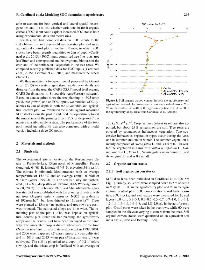
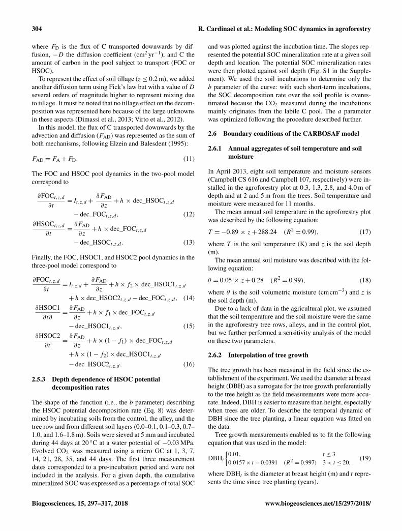
Figure 1. Soil organic carbon content in both the agroforestry andagricultural control plot. Associated errors are standard errors. N =93 in the control, N = 40 in the agroforestry tree row, N = 60 inthe agroforestry alley. Data from Cardinael et al. (2015b).

120 kgNha−1 yr−1. Crop residues (wheat straw) are also ex-ported, but about 25 % remains on the soil. Tree rows arecovered by spontaneous herbaceous vegetation. Two suc-cessive herbaceous vegetation types occur during the year,one in summer and one in winter. The summer vegetation ismainly composed of Avena fatua L. and is 1.5 m tall. In win-ter, the vegetation is a mix of Achillea millefolium L., Gal-ium aparine L., Vicia L., Ornithogalum umbellatum L., andAvena fatua L. and is 0.2 m tall.

2.2 Organic carbon stocks

2.2.1 Soil organic carbon stocks

SOC data have been published in Cardinael et al. (2015b;Fig. 1). Briefly, soil cores were sampled down to 2 m of depthin May 2013, 100 in the agroforestry plot, and 93 in the agri-cultural control plot. SOC concentrations, soil bulk densi-ties, SOC stocks, and soil texture were measured for 10 soillayers (0.0–0.1, 0.1–0.3, 0.3–0.5, 0.5–0.7, 0.7–1.0, 1.0–1.2,1.2–1.4, 1.4–1.6, 1.6–1.8, and 1.8–2.0 m). In the agroforestryplot, 40 soil cores were taken in the tree rows, while 60 weresampled in the alleys at varying distances from the trees. Soilorganic carbon stocks were quantified on an equivalent soilmass basis (Ellert and Bettany, 1995).

www.biogeosciences.net/15/297/2018/ Biogeosciences, 15, 297–317, 2018


Table 1. Synthesis of the different field and laboratory data available or measured and their sources.

Description of the data Source

Soil texture, bulk densities, SOC stocks Cardinael et al. (2015b)Soil temperature and soil moisture MeasuredTree growth (DBH) MeasuredTree wood density Talbot (2011)Tree fine root biomass Cardinael et al. (2015a)Tree fine root turnover Germon et al. (2016)Crop yield and crop ABG biomass Dufour et al. (2013) and measuredCrop root biomass Prieto et al. (2015) and measuredTree row herbaceous vegetation – ABG biomass MeasuredTree row herbaceous vegetation – root biomass MeasuredBiomass carbon concentrations MeasuredPotential decomposition rate of roots Prieto et al. (2016)HSOC potential decomposition rate Measured

DBH: diameter at breast height; ABG: aboveground; OC: organic carbon; HSOC: humified soil organic carbon.

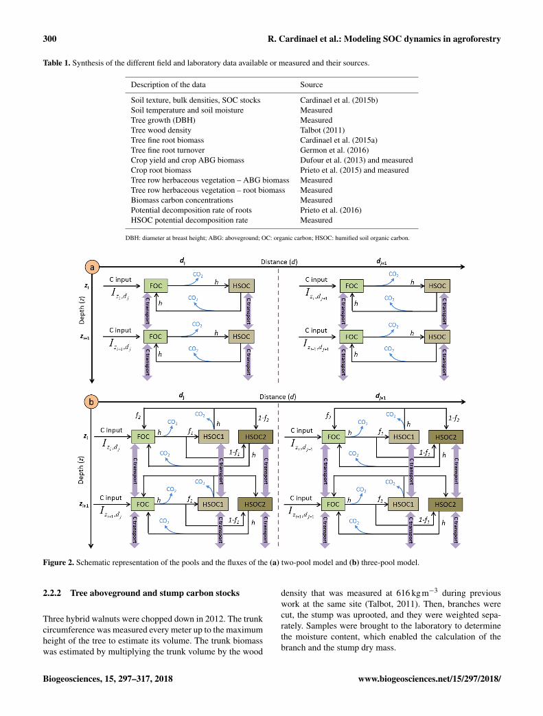
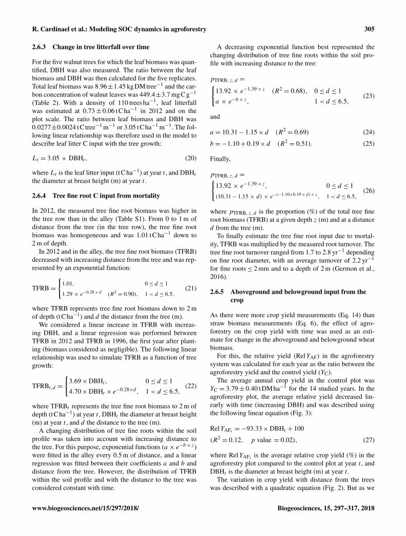
Figure 2. Schematic representation of the pools and the fluxes of the (a) two-pool model and (b) three-pool model.

2.2.2 Tree aboveground and stump carbon stocks

Three hybrid walnuts were chopped down in 2012. The trunkcircumference was measured every meter up to the maximumheight of the tree to estimate its volume. The trunk biomasswas estimated by multiplying the trunk volume by the wood

density that was measured at 616 kgm−3 during previouswork at the same site (Talbot, 2011). Then, branches werecut, the stump was uprooted, and they were weighted sepa-rately. Samples were brought to the laboratory to determinethe moisture content, which enabled the calculation of thebranch and the stump dry mass.



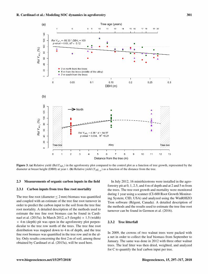
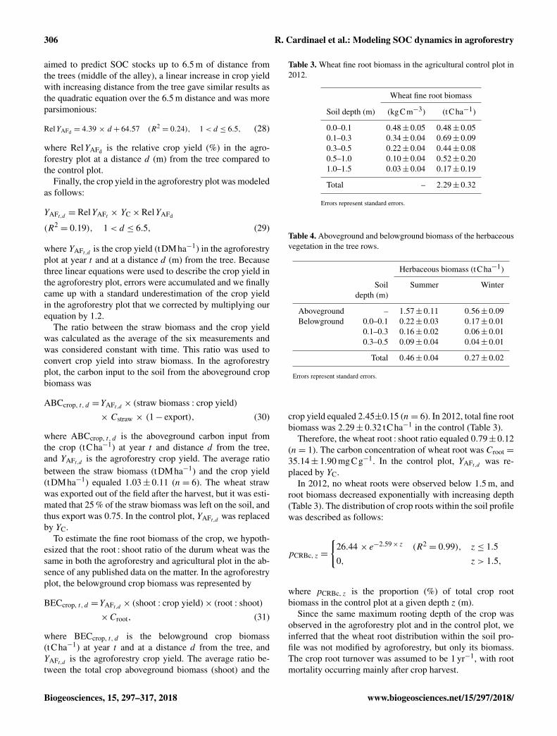
Figure 3. (a) Relative yield (RelYAFt ) in the agroforestry plot compared to the control plot as a function of tree growth, represented by thediameter at breast height (DBH) at year t . (b) Relative yield (YAFt,d ) as a function of the distance from the tree.

2.3 Measurements of organic carbon inputs in the field

2.3.1 Carbon inputs from tree fine root mortality

The tree fine root (diameter≤ 2 mm) biomass was quantifiedand coupled with an estimate of the tree fine root turnover inorder to predict the carbon input to the soil from the tree fineroot mortality. A detailed description of the methods used toestimate the tree fine root biomass can be found in Cardi-nael et al. (2015a). In March 2012, a 5 (length)× 1.5 (width)× 4 m (depth) pit was open in the agroforestry plot perpen-dicular to the tree row north of the trees. The tree fine rootdistribution was mapped down to 4 m of depth, and the treefine root biomass was quantified in the tree row and in the al-ley. Only results concerning the first 2 m of soil, among thoseobtained by Cardinael et al. (2015a), will be used here.

In July 2012, 16 minirhizotrons were installed in the agro-forestry pit at 0, 1, 2.5, and 4 m of depth and at 2 and 5 m fromthe trees. The tree root growth and mortality were monitoredduring 1 year using a scanner (CI-600 Root Growth Monitor-ing System; CID, USA) and analyzed using the WinRHIZOTron software (Régent, Canada). A detailed description ofthe methods and the results used to estimate the tree fine rootturnover can be found in Germon et al. (2016).

2.3.2 Tree litterfall

In 2009, the crowns of two walnut trees were packed witha net in order to collect the leaf biomass from September toJanuary. The same was done in 2012 with three other walnuttrees. The leaf litter was then dried, weighted, and analyzedfor C to quantify the leaf carbon input per tree.



2.3.3 Aboveground and belowground input from thecrop

Since the tree planting in 1995, the crop yield was measured14 times (in 1995, 2000, 2002, 2003, 2004, 2005, 2007, 2008,2009, 2010, 2011, 2012, 2013, and 2014), while the wheatstraw biomass and the total aboveground biomass were mea-sured 6 times (in 2007, 2008, 2009, 2011, 2012, and 2014)in both the control and the agroforestry plot (Dufour et al.,2013) using sampling subplots of 1 m2 each. In the controlplot, five subplots have been sampled, while in the agro-forestry plot five transects have been sampled. Each transectwas made up of three subplots, 2 m north from the tree, 2 msouth from the tree, and 6.5 m from the tree (middle of thealley). In March 2012, a 2 m deep pit was opened in the agri-cultural control plot (Prieto et al., 2015), and the root biomasswas quantified to the maximum rooting depth (1.5 m). Theroot : shoot ratio of durum wheat was measured in the con-trol plot. We assumed that the crop root biomass turns outonce a year after the crop harvest.

2.3.4 Aboveground and belowground input from thetree row herbaceous vegetation

As two types of herbaceous vegetation grow in the tree rowsduring the year, samples were taken in summer and winter.In late June 2014, 12 subplots of 1 m2 each were positionedin the tree rows around four walnut trees. In January 2015,six subplots of 1 m2 each were positioned in the tree rowsaround two walnut trees. The middle of each subplot was lo-cated at 1, 2, and 3 m, respectively, from the selected walnuttree. All the aboveground vegetation was collected in eachsquare. In the middle of each subplot, root biomass was sam-pled with a cylindrical soil corer (inner diameter of 8 cm).Soil was taken at three soil layers, 0.0–0.1, 0.1–0.3, and 0.3–0.5 m. In the laboratory, soil was gently washed with waterthrough a 2 mm mesh sieve, and roots were collected. Rootsfrom the herbaceous vegetation were easily separated man-ually from walnut roots, as they were soft and yellow com-pared to walnuts roots that were black. After being sortedout from the soil and cleaned, the root biomass was dried at40 ◦C and measured.

2.4 Carbon concentration measurements

All organic carbon measurements were performed witha CHN elemental analyzer (Carlo Erba NA-2000, Milan,Italy) after samples were oven-dried at 40 ◦C for 48 h (Ta-ble 2). Dry biomasses (tDMha−1) of each organic matter in-put were multiplied by their respective organic carbon con-centrations (mgC g−1) to calculate organic carbon stocks(tCha−1).

2.5 General description of the CARBOSAF model

2.5.1 Organic carbon decomposition

We adapted a model developed by Guenet et al. (2013) inwhich total SOC is split in two pools, the FOC and the humi-fied soil organic carbon (HSOC) for each soil layer (Fig. 1a).Input to the FOC pool comes from the plant litter and the dis-tribution of this input within the profile is assumed to dependupon depth from the surface (z), distance from the tree (d),and time (t). Equations describing inputs to the FOC pool(It,z,d ) at a given time, depth, and distance are fully explainedin Sect. 3.

The FOC mineralization is assumed to be governed byfirst-order kinetics, being proportional to the FOC pool, asgiven by

dec_FOCt,z,d = − kFOC × FOCt,z,d × fclay, z× fmoist, z

× ftemp, z, (1)

where FOCt,z,d is the FOC carbon pool (kgCm−2) at a giventime (t , in years), depth (z, in m), and distance (d, in m), andkFOC is its decomposition rate. The potential decompositionrates of the different plant materials were assessed with a 16-week incubation experiment during a companion study at thesite (Prieto et al., 2016). The decomposition rate kFOC wasweighted by the respective contribution of each type of plantlitter as a function of the tree age, soil depth, and distancefrom the tree. The rate modifiers fclay, z, fmoist, z, and ftemp, zare functions depending respectively on the clay content, soilmoisture, and soil temperature at a given depth z and rangebetween 0 and 1.

The fclay function originated from the CENTURY model(Parton et al., 1987):

fclay, z = 1− 0.75 × Clayz, (2)

where Clayz is the clay fraction (ranging between 0 and 1) ofthe soil at a given depth z.

The fmoist, z function originated from the meta-analysis ofMoyano et al. (2012) and is affected by soil properties (claycontent, SOC content). Briefly, the authors fitted linear mod-els on 310 soil incubations to describe the effect of soil mois-ture on decomposition. Then, they normalized such linearmodels between 0 and 1 to apply these functions to classi-cal first-order kinetics. All details are described in Moyanoet al. (2012). To save computing time, we calculated fmoist, zonly once using measured SOC stocks instead of using mod-eled SOC stocks and repeated the calculation at each timestep.

The temperature sensitivity of the soil respiration is ex-pressed as Q10:

ftemp, z =Q

tempz−tempopt10

10 , (3)

with tempz being the soil temperature in K at each soil depthz and tempopt a parameter fixed to 304.15 K. The Q10 value



Table 2. Organic carbon concentrations and C : N ratio of the different types of biomass.

Type of biomass Organic C concentration C : N Number of(mgCg−1) replicates

Walnut trunk 445.7± 1.0 159.1± 25.2 3Walnut branches 428.6± 1.7 62.2± 11.7 3Wheat straw 433.2± 0.7 55.5± 2.1 5Wheat root 351.4± 19 24.8± 2.1 8Walnut leaf 449.4± 3.7 49.1± 0.4 3Walnut fine root 437.0± 3.3 28.6± 3.4 8Summer vegetation (ABG) 448.4± 1.9 37.8± 2.2 5Summer vegetation (roots) 314.5± 8.3 33.8± 1.7 6Winter vegetation (ABG) 447.7± 5.3 11.2± 0.4 3Winter vegetation (roots) 397.4± 5.0 24.7± 0.7 3

The organic matter called “vegetation” stands for the herbaceous vegetation that grows in the tree row. ABG:aboveground. Errors represent standard errors.

was fixed to 2, a classical value used in models (Davidsonand Janssens, 2006).

Once the FOC is decomposed, a fraction is humified (h)and another is respired as CO2 (1−h) (Fig. 2a) followingEqs. (4) and (5).

Humified FOCt,z,d = h× dec_FOCt,z,d (4)Respired FOCt,z,d = (1−h)× dec_FOCt,z,d (5)

Two mathematical approaches are available in the model todescribe the mineralization of HSOC: a first-order kinetics,as given by Eq. (6), or an approach developed by Wutzler andReichstein (2008) and by Guenet et al. (2013) introducing thepriming effect, i.e., the mineralization of HSOC depends onFOC availability, and given by Eq. (7):

dec_HSOCt,z,d =− kHSOC, z×HSOCt,z,d × fmoist, z (6)× ftemp, z,

dec_HSOCt,z,d =− kHSOC, z×HSOCt,z,d (7)

×

(1− e−PE×FOCt,z,d

)× fmoist, z× ftemp, z,

where HSOCt,z,d is the humified SOC carbon pool at a giventime (t , in years), depth (z, in m), and distance (d, in m),kHSOC, z is its decomposition rate (yr−1) at a given depthz, and PE is the priming effect parameter. The parametersfmoist, z and ftemp, z are functions depending respectively onsoil moisture and soil temperature at a given depth z and af-fecting the decomposition rate of HSOC. They correspondto the moisture equation from Moyano et al. (2012) and toEq. (3), respectively. The decomposition rate kHSOC, z is anexponential law depending on soil depth (z) as shown byan incubation study (see paragraph on HSOC decompositionrate in Sect. 2):

kHSOC, z = a× e−b× z. (8)

The b parameter of this equation represented the ratio of la-bile C/stable C within the HSOC pool. The effect of clay on

HSOC decomposition was implicitly taken into account inthis equation as clay content increased with soil depth.

A fraction of decomposed HSOC returns to the FOC as-suming that part of the HSOC decomposition products is aslabile as FOC (h) and another is respired as CO2 (Fig. 2a) inthe two-pool model.

Finally, we also developed an alternative version of themodel with three pools by splitting the HSOC pools intotwo pools with different turnover rates, HSOC2 being morestabilized than HSOC1 (Fig. 2b). The non-respired decom-posed FOC is split between HSOC1 and HSOC2 follow-ing a parameter f1. The non-respired decomposed HSOC1is split between HSOC2 and FOC following a parameterf2, whereas non-respired decomposed HSOC2 is only redis-tributed into the FOC pools. The decomposition of HSOC1and HSOC2 both follow Eq. (8) but with different parametervalues for a.

2.5.2 Carbon transport mechanisms

The transport of C between the different soil layers was rep-resented by both advection and diffusion mechanisms (Elzeinand Balesdent, 1995), which have been shown to describe theC transport in soils well (Bruun et al., 2007; Guenet et al.,2013). The advection represents the C transport due to wa-ter infiltration in the soil, while the diffusion represents theC transport due to fauna activity. The same transport coeffi-cients were applied to the two C pools, FOC and HSOC.

The advection is defined by

FA = A × C, (9)

where FA is the flux of C transported downwards by advec-tion, and A is the advection rate (mmyr−1).

The diffusion is represented by Fick’s law:

FD =−D×∂2C∂z2 , (10)



where FD is the flux of C transported downwards by dif-fusion, −D the diffusion coefficient (cm2 yr−1), and C theamount of carbon in the pool subject to transport (FOC orHSOC).

To represent the effect of soil tillage (z ≤ 0.2 m), we addedanother diffusion term using Fick’s law but with a value ofDseveral orders of magnitude higher to represent mixing dueto tillage. It must be noted that no tillage effect on the decom-position was represented here because of the large unknownsin these aspects (Dimassi et al., 2013; Virto et al., 2012).

In this model, the flux of C transported downwards by theadvection and diffusion (FAD) was represented as the sum ofboth mechanisms, following Elzein and Balesdent (1995):

FAD = FA+FD. (11)

The FOC and HSOC pool dynamics in the two-pool modelcorrespond to

∂FOCt,z,d∂t

= It,z,d +∂FAD

∂z+h × dec_HSOCt,z,d

− dec_FOCt,z,d , (12)∂HSOCt,z,d

∂t=∂FAD

∂z+h × dec_FOCt,z,d

− dec_HSOCt,z,d . (13)

Finally, the FOC, HSOC1, and HSOC2 pool dynamics in thethree-pool model correspond to

∂FOCt,z,d∂t

= It,z,d +∂FAD

∂z+h× f2× dec_HSOC1t,z,d

+h× dec_HSOC2t,z,d − dec_FOCt,z,d , (14)∂HSOC1∂t∂

=∂FAD

∂z+h× f1× dec_FOCt,z,d

− dec_HSOC1t,z,d , (15)∂HSOC2∂t

=∂FAD

∂z+h× (1− f1) × dec_FOCt,z,d

+h× (1− f2)× dec_HSOC1t,z,d− dec_HSOC2t,z,d . (16)

2.5.3 Depth dependence of HSOC potentialdecomposition rates

The shape of the function (i.e., the b parameter) describingthe HSOC potential decomposition rate (Eq. 8) was deter-mined by incubating soils from the control, the alley, and thetree row and from different soil layers (0.0–0.1, 0.1–0.3, 0.7–1.0, and 1.6–1.8 m). Soils were sieved at 5 mm and incubatedduring 44 days at 20 ◦C at a water potential of −0.03 MPa.Evolved CO2 was measured using a micro GC at 1, 3, 7,14, 21, 28, 35, and 44 days. The first three measurementdates corresponded to a pre-incubation period and were notincluded in the analysis. For a given depth, the cumulativemineralized SOC was expressed as a percentage of total SOC

and was plotted against the incubation time. The slopes rep-resented the potential SOC mineralization rate at a given soildepth and location. The potential SOC mineralization rateswere then plotted against soil depth (Fig. S1 in the Supple-ment). We used the soil incubations to determine only theb parameter of the curve: with such short-term incubations,the SOC decomposition rate over the soil profile is overes-timated because the CO2 measured during the incubationsmainly originates from the labile C pool. The a parameterwas optimized following the procedure described further.

2.6 Boundary conditions of the CARBOSAF model

2.6.1 Annual aggregates of soil temperature and soilmoisture

In April 2013, eight soil temperature and moisture sensors(Campbell CS 616 and Campbell 107, respectively) were in-stalled in the agroforestry plot at 0.3, 1.3, 2.8, and 4.0 m ofdepth and at 2 and 5 m from the trees. Soil temperature andmoisture were measured for 11 months.

The mean annual soil temperature in the agroforestry plotwas described by the following equation:

T =−0.89 × z+ 288.24 (R2= 0.99), (17)

where T is the soil temperature (K) and z is the soil depth(m).

The mean annual soil moisture was described with the fol-lowing equation:

θ = 0.05 × z+ 0.28 (R2= 0.99), (18)

where θ is the soil volumetric moisture (cmcm−3) and z isthe soil depth (m).

Due to a lack of data in the agricultural plot, we assumedthat the soil temperature and the soil moisture were the samein the agroforestry tree rows, alleys, and in the control plot,but we further performed a sensitivity analysis of the modelon these two parameters.

2.6.2 Interpolation of tree growth

The tree growth has been measured in the field since the es-tablishment of the experiment. We used the diameter at breastheight (DBH) as a surrogate for the tree growth preferentiallyto the tree height as the field measurements were more accu-rate. Indeed, DBH is easier to measure than height, especiallywhen trees are older. To describe the temporal dynamic ofDBH since the tree planting, a linear equation was fitted onthe data.

Tree growth measurements enabled us to fit the followingequation that was used in the model:

DBHt{

0.01, t ≤ 30.0157× t − 0.0391 (R2

= 0.997) 3< t ≤ 20,(19)

where DBHt is the diameter at breast height (m) and t repre-sents the time since tree planting (years).



2.6.3 Change in tree litterfall over time

For the five walnut trees for which the leaf biomass was quan-tified, DBH was also measured. The ratio between the leafbiomass and DBH was then calculated for the five replicates.Total leaf biomass was 8.96±1.45 kgDMtree−1 and the car-bon concentration of walnut leaves was 449.4±3.7 mgCg−1

(Table 2). With a density of 110 treesha−1, leaf litterfallwas estimated at 0.73± 0.06 tCha−1 in 2012 and on theplot scale. The ratio between leaf biomass and DBH was0.0277±0.0024 tC tree−1 m−1 or 3.05 tCha−1 m−1. The fol-lowing linear relationship was therefore used in the model todescribe leaf litter C input with the tree growth:

Lt = 3.05 × DBHt , (20)

where Lt is the leaf litter input (tCha−1) at year t , and DBHtthe diameter at breast height (m) at year t .

2.6.4 Tree fine root C input from mortality

In 2012, the measured tree fine root biomass was higher inthe tree row than in the alley (Table S1). From 0 to 1 m ofdistance from the tree (in the tree row), the tree fine rootbiomass was homogeneous and was 1.01 tCha−1 down to2 m of depth.

In 2012 and in the alley, the tree fine root biomass (TFRB)decreased with increasing distance from the tree and was rep-resented by an exponential function:

TFRB=

{1.01, 0≤ d ≤ 1

1.29 × e−0.28× d (R2= 0.90), 1< d ≤ 6.5,

(21)

where TFRB represents tree fine root biomass down to 2 mof depth (tCha−1) and d the distance from the tree (m).

We considered a linear increase in TFRB with increas-ing DBH, and a linear regression was performed betweenTFRB in 2012 and TFRB in 1996, the first year after plant-ing (biomass considered as negligible). The following linearrelationship was used to simulate TFRB as a function of treegrowth:

TFRBt,d =

{3.69×DBHt , 0≤ d ≤ 1

4.70×DBHt × e−0.28×d , 1< d ≤ 6.5,(22)

where TFRBt represents the tree fine root biomass to 2 m ofdepth (tCha−1) at year t , DBHt the diameter at breast height(m) at year t , and d the distance to the tree (m).

A changing distribution of tree fine roots within the soilprofile was taken into account with increasing distance tothe tree. For this purpose, exponential functions (a × e−b× z)were fitted in the alley every 0.5 m of distance, and a linearregression was fitted between their coefficients a and b anddistance from the tree. However, the distribution of TFRBwithin the soil profile and with the distance to the tree wasconsidered constant with time.

A decreasing exponential function best represented thechanging distribution of tree fine roots within the soil pro-file with increasing distance to the tree:

pTFRB, z, d ={13.92 × e−1.39× z (R2

= 0.68), 0≤ d ≤ 1

a × e−b× z, 1< d ≤ 6.5,(23)

and

a = 10.31− 1.15× d (R2= 0.69) (24)

b =−1.10+ 0.19× d (R2= 0.51). (25)

Finally,

pTFRB, z, d ={13.92 × e−1.39× z, 0≤ d ≤ 1

(10.31− 1.15 × d) × e−(−1.10+0.19× d)× z, 1< d ≤ 6.5,(26)

where pTFRB, z, d is the proportion (%) of the total tree fineroot biomass (TFRB) at a given depth z (m) and at a distanced from the tree (m).

To finally estimate the tree fine root input due to mortal-ity, TFRB was multiplied by the measured root turnover. Thetree fine root turnover ranged from 1.7 to 2.8 yr−1 dependingon fine root diameter, with an average turnover of 2.2 yr−1

for fine roots≤ 2 mm and to a depth of 2 m (Germon et al.,2016).

2.6.5 Aboveground and belowground input from thecrop

As there were more crop yield measurements (Eq. 14) thanstraw biomass measurements (Eq. 6), the effect of agro-forestry on the crop yield with time was used as an esti-mate for change in the aboveground and belowground wheatbiomass.

For this, the relative yield (RelYAF) in the agroforestrysystem was calculated for each year as the ratio between theagroforestry yield and the control yield (YC).

The average annual crop yield in the control plot wasYC = 3.79± 0.40 tDMha−1 for the 14 studied years. In theagroforestry plot, the average relative yield decreased lin-early with time (increasing DBH) and was described usingthe following linear equation (Fig. 3):

RelYAFt =−93.33×DBHt + 100

(R2= 0.12, p value = 0.02), (27)

where RelYAFt is the average relative crop yield (%) in theagroforestry plot compared to the control plot at year t , andDBHt is the diameter at breast height (m) at year t .

The variation in crop yield with distance from the treeswas described with a quadratic equation (Fig. 2). But as we



aimed to predict SOC stocks up to 6.5 m of distance fromthe trees (middle of the alley), a linear increase in crop yieldwith increasing distance from the tree gave similar results asthe quadratic equation over the 6.5 m distance and was moreparsimonious:

RelYAFd = 4.39 × d + 64.57 (R2= 0.24), 1< d ≤ 6.5, (28)

where RelYAFd is the relative crop yield (%) in the agro-forestry plot at a distance d (m) from the tree compared tothe control plot.

Finally, the crop yield in the agroforestry plot was modeledas follows:

YAFt,d = RelYAFt × YC×RelYAFd

(R2= 0.19), 1< d ≤ 6.5, (29)

where YAFt,d is the crop yield (tDMha−1) in the agroforestryplot at year t and at a distance d (m) from the tree. Becausethree linear equations were used to describe the crop yield inthe agroforestry plot, errors were accumulated and we finallycame up with a standard underestimation of the crop yieldin the agroforestry plot that we corrected by multiplying ourequation by 1.2.

The ratio between the straw biomass and the crop yieldwas calculated as the average of the six measurements andwas considered constant with time. This ratio was used toconvert crop yield into straw biomass. In the agroforestryplot, the carbon input to the soil from the aboveground cropbiomass was

ABCcrop, t, d =YAFt,d × (straw biomass : crop yield)× Cstraw × (1− export), (30)

where ABCcrop, t, d is the aboveground carbon input fromthe crop (tCha−1) at year t and distance d from the tree,and YAFt,d is the agroforestry crop yield. The average ratiobetween the straw biomass (tDMha−1) and the crop yield(tDMha−1) equaled 1.03± 0.11 (n= 6). The wheat strawwas exported out of the field after the harvest, but it was esti-mated that 25 % of the straw biomass was left on the soil, andthus export was 0.75. In the control plot, YAFt,d was replacedby YC.

To estimate the fine root biomass of the crop, we hypoth-esized that the root : shoot ratio of the durum wheat was thesame in both the agroforestry and agricultural plot in the ab-sence of any published data on the matter. In the agroforestryplot, the belowground crop biomass was represented by

BECcrop, t, d =YAFt,d × (shoot : crop yield)× (root : shoot)×Croot, (31)

where BECcrop, t, d is the belowground crop biomass(tCha−1) at year t and at a distance d from the tree, andYAFt,d is the agroforestry crop yield. The average ratio be-tween the total crop aboveground biomass (shoot) and the

Table 3. Wheat fine root biomass in the agricultural control plot in2012.

Wheat fine root biomass

Soil depth (m) (kgCm−3) (tCha−1)

0.0–0.1 0.48± 0.05 0.48± 0.050.1–0.3 0.34± 0.04 0.69± 0.090.3–0.5 0.22± 0.04 0.44± 0.080.5–1.0 0.10± 0.04 0.52± 0.201.0–1.5 0.03± 0.04 0.17± 0.19

Total – 2.29± 0.32

Errors represent standard errors.

Table 4. Aboveground and belowground biomass of the herbaceousvegetation in the tree rows.

Herbaceous biomass (tCha−1)

Soil Summer Winterdepth (m)

Aboveground – 1.57± 0.11 0.56± 0.09Belowground 0.0–0.1 0.22± 0.03 0.17± 0.01

0.1–0.3 0.16± 0.02 0.06± 0.010.3–0.5 0.09± 0.04 0.04± 0.01

Total 0.46± 0.04 0.27± 0.02

Errors represent standard errors.

crop yield equaled 2.45±0.15 (n= 6). In 2012, total fine rootbiomass was 2.29± 0.32 tCha−1 in the control (Table 3).

Therefore, the wheat root : shoot ratio equaled 0.79±0.12(n= 1). The carbon concentration of wheat root was Croot =

35.14± 1.90 mgCg−1. In the control plot, YAFt,d was re-placed by YC.

In 2012, no wheat roots were observed below 1.5 m, androot biomass decreased exponentially with increasing depth(Table 3). The distribution of crop roots within the soil profilewas described as follows:

pCRBc, z =

{26.44 × e−2.59× z (R2

= 0.99), z ≤ 1.5

0, z > 1.5,

where pCRBc, z is the proportion (%) of total crop rootbiomass in the control plot at a given depth z (m).

Since the same maximum rooting depth of the crop wasobserved in the agroforestry plot and in the control plot, weinferred that the wheat root distribution within the soil pro-file was not modified by agroforestry, but only its biomass.The crop root turnover was assumed to be 1 yr−1, with rootmortality occurring mainly after crop harvest.



2.6.6 Aboveground and belowground input fromherbaceous vegetation in the tree rows

The distance from the trees had no effect on the above-ground and belowground biomass of the herbaceous veg-etation (data not shown), and therefore average values arepresented. The summer aboveground biomass was almost3 times higher than in winter, whereas the belowgroundbiomass was 2 times higher (Table 4). The total above-ground carbon input was 2.13± 0.14 tCha−1 yr−1 and thetotal belowground carbon input was 0.74±0.05 tCha−1 yr−1

to 0.5 m of depth.The belowground carbon input from the tree row vegeta-

tion (BECveg, z, tC ha−1) at a given depth z (m) was describedby the following equation:

BECveg, z =

{0.44 × e−3.12× z z ≤ 1.5

0, z > 1.5.

We assumed for simplification that the aboveground and be-lowground biomasses of the herbaceous vegetation in the treerow were constant over time.

2.7 Optimization procedure

Depending on the model variant, four to five parameters wereoptimized with a gradient-based statistical method (Santarenet al., 2007; Tarantola, 1987, 2005) using measured SOCstocks from the control plot only. These parameters were Athe advection rate, D the diffusion coefficient, h the humifi-cation yield, a the coefficient of the kHSOC rate from Eq. (10),and PE the priming coefficient. These four to five parame-ters were calibrated so that equilibrium SOC stocks, i.e., after5000 years of simulation, equaled SOC stocks of the controlplot in 2013. The associated uncertainty was estimated withthe 93 soil cores sampled in the control plot (see Sect. 2.2.1).Due to a lack of relevant data, we assumed that the climateand the land use were the same for the last 5000 years andthat SOC stocks in the control plot were at equilibrium at thetime of measurement. Therefore, SOC stocks at the end ofthe 5000 years of simulation equaled SOC stocks in the con-trol plot. Three different calibrations were performed corre-sponding to the three model variants that were used: one cal-ibration with the two-pool model without the priming effect,one calibration with the two-pool model with the priming ef-fect, and one calibration with the three-pool model.

Each model variant was fitted to the control SOC stockdata using a curve-fitting method described in Taran-tola (1987), after a conversion from SOC stocks in kgCm−2

to SOC stocks in kg m−3 due to the different soil layer thick-nesses. We aimed to find a parameter set that minimizesthe distance between model outputs and the correspond-ing observations considering model and data uncertaintiesand starting parameter information. With the assumption ofGaussian errors for both the observations and the starting pa-

rameters, the optimal parameter set corresponds to the mini-mum of the cost function J(x):

J(x)=0.5×[(y−H(x))t ×R−1

× (y−H(x))+ (x− xb)t

×P−1b × (x− xb)

], (32)

which contains both the mismatch between modeled and ob-served SOC stock and the mismatch between starting and op-timized parameters; x is the vector of unknown parameters,xb the vector of starting parameter values fixed for each opti-mization procedure, H() the model, and y the vector of obser-vations. The covariance matrices Pb and R describe a prioriuncertainties in parameters and observations, respectively.Both matrices are diagonal as we suppose the observation un-certainties and the parameter uncertainties to be independent.The covariance matrices Pb are presented in Table S2. To de-termine an optimal set of parameters that minimizes J(x), weused the BFGS gradient-based algorithm (Tarantola, 1987).For each model variant, we performed 30 optimizations withdifferent starting parameter values to check that the resultsdid not correspond to a local minimum. As the BFGS algo-rithm does not directly calculate the variance of posteriors,they were quantified using the curvature cost function at itsminimum once it was reached (Santaren et al., 2007).

2.8 Comparison of models

Model predictions with and without the priming effect werecompared by calculating the coefficients of determination,root mean square error (RMSE), and Bayesian informationcriteria (BIC).

RMSE=

√√√√ 1N

N∑i=1(xi − x)

2, (33)

where i is the number of observations (1 to N ), xi is thepredicted value, and x is the mean observed value.

BIC= k × ln(N)− 2× ln(L̂), (34)

where N is the number of observations, k is the number ofmodel parameters, and L̂ is the maximized value of the like-lihood function of the model (Schwarz, 1978).

The model was run at a yearly time step using mean an-nual soil temperature and moisture and annual C inputs tothe soil. In the agroforestry plot, the model was run from theground (0 m) to 2 m of depth and from the tree (0 m) to 6.5 mfrom the tree (middle of the alley). The model was appliedseparately across locations of a tree-distance gradient hav-ing varying OC inputs, and each soil column was consideredindependent from another. SOC pools were initialized aftera spin-up of 5000 years in the control plot. At t0, SOC stocksin the agroforestry plot therefore equaled SOC stocks of thecontrol plot. The model was then run from t0 to t18 (years)



after tree planting. The spatial resolution was 0.1 m both ver-tically and horizontally. The model was developed using R3.1.1 (R Development Core Team, 2013). Partial differentialequations were solved using the R package deSolve and theode.1D method (Soetaert et al., 2010).

3 Results

3.1 Organic carbon inputs and SOC stocks: a synthesisfrom field measurements

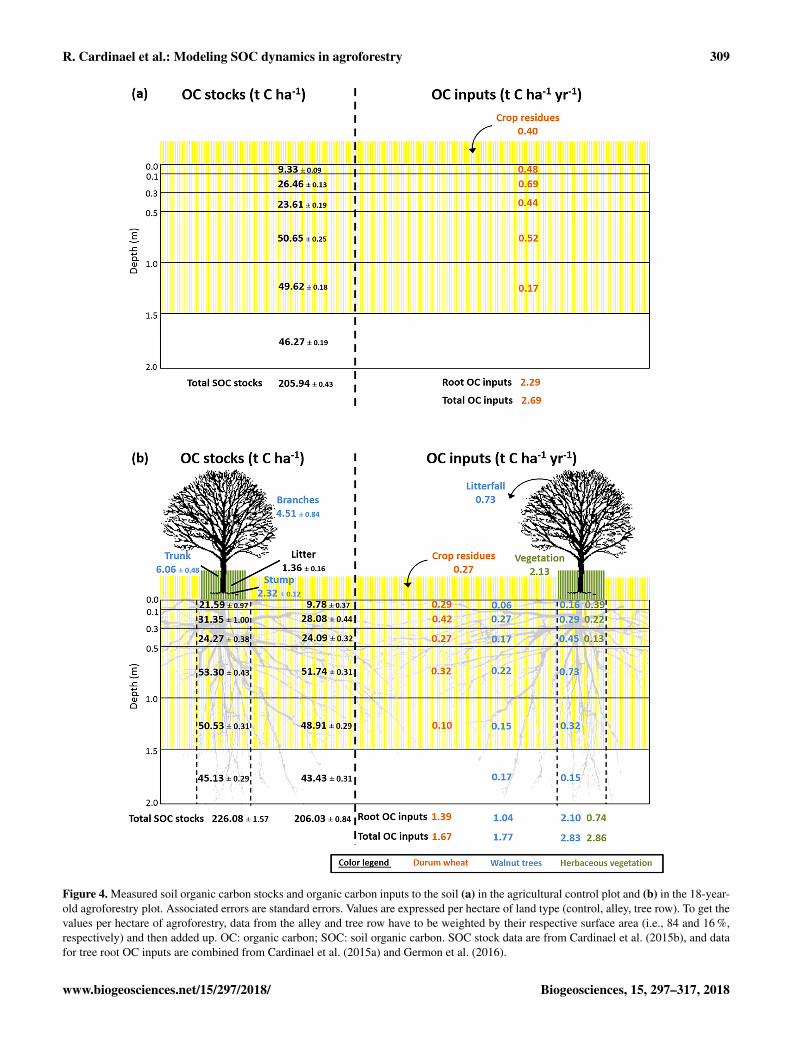
In the alleys of the 18-year-old agroforestry system, mea-sured organic carbon (OC) inputs from the crop residues androots were reduced compared to the control plot due a lowercrop yield (Fig. 4). This reduction in crop OC inputs was off-set by OC inputs from the tree roots and tree litterfall. Totalroot OC inputs in the alleys (crop+ tree roots) and in the con-trol plot (crop roots) were very similar, respectively 2.43 and2.29 tCha−1 yr−1. Alleys received 0.60 tCha−1 yr−1 moretotal aboveground biomass (crop residues+ tree litterfall)than the control, which was added to the plough layer. Treerows received 2.35 tCha−1 yr−1 more C inputs in the first0.3 m of soil compared to the control plot, mainly fromthe herbaceous vegetation. Down the whole soil profile, treerows received 2 times more OC inputs compared to the con-trol plot (Fig. 4) and 65 % more than alleys. Overall, theagroforestry plot had 41 % more OC inputs to the soil thanthe control plot to 2 m of depth (3.80 tCha−1 yr−1 comparedto 2.69 tCha−1 yr−1). In the agroforestry plot, the largestaboveground OC input to the soil comes from the herbaceousvegetation, and not from the trees. In the control plot, 85 %of OC input is wheat root litter. In the agroforestry plot, rootinputs represent 71 % of OC inputs in the alleys and 50 % inthe tree rows.

In the first 0.3 m of soil, SOC stocks were significantlyhigher in the alleys than in the control plot, but the differ-ence was small (2.1± 0.6 tCha−1). Between 0.3 and 1.0 m,the difference in SOC stocks was smaller but still significant.However, between 1 and 2 m of depth, SOC stocks were sig-nificantly lower in the alleys than in the control. As a con-sequence, there was no significant difference in total SOCstocks between the two locations down the whole soil profile.In the tree rows, topsoil organic carbon stocks (0.0–0.3 m)were much higher than in the control (+17.0± 1.4 tCha−1).This positive difference of SOC stocks decreased with depthbut remained significantly positive down to 1.5 m of depth.The opposite was observed between 1.5 and 2.0 m of depth.The delta value of total SOC stocks between the tree rowsand the control plot was 20.1± 1.6 tCha−1. On the plotscale, total SOC stocks were significantly higher in the agro-forestry plot compared to the control plot down to 2 m ofdepth (+3.3± 0.9 t Cha−1).

3.2 HSOC decomposition rate

The soil incubation experiment showed that the HSOC min-eralization rate decreased exponentially with depth (Fig. S1in the Supplement) and could be described with

kHSOC, z = 6.114 × e−1.37× z (R2= 0.76), (35)

where z is the soil depth (m), and the a (yr−1) coefficient(a = 6.114) was further optimized (Table 5).

3.3 Modeling results

3.3.1 Optimized parameters and correlation matrix

The optimized parameters and their starting parameter modesare presented in Table 5. For the two-pool model without thepriming effect, the most important correlation was observedbetween h and A, which control the humification and thetransport by advection. Concerning the two-pool model withthe priming effect, the most important correlations were ob-served between h and PE, which control the effect of the FOCon HSOC decomposition, and between h and A. A and PEwere also positively correlated (Fig. S2 in the Supplement).For the three-pool model, f1 and f2 were by definition neg-atively correlated, but f2 and A were also correlated. Con-sidering the method used to optimize the parameters, theseimportant correlation factors hinder the presentation of themodel output within an envelope. Therefore, we presentedthe model results using the optimized parameter without anyenvelope.

3.3.2 Modeled SOC stocks

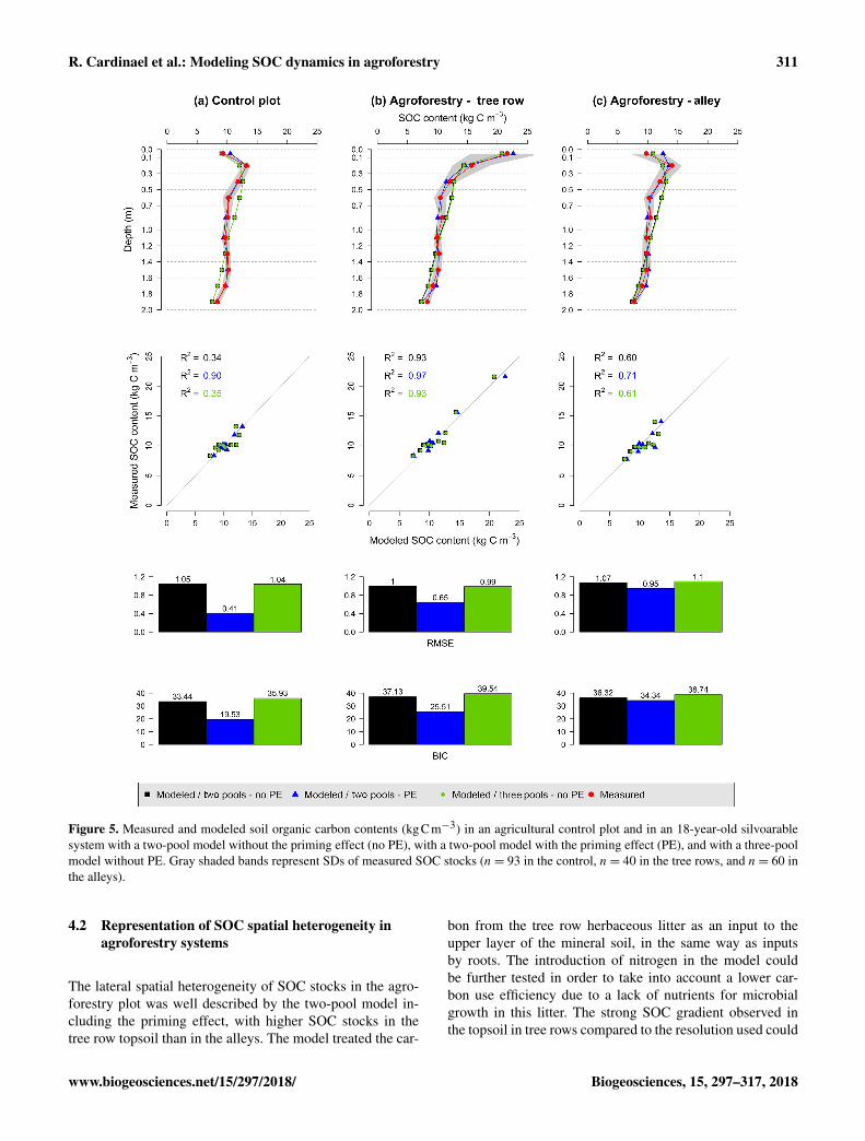
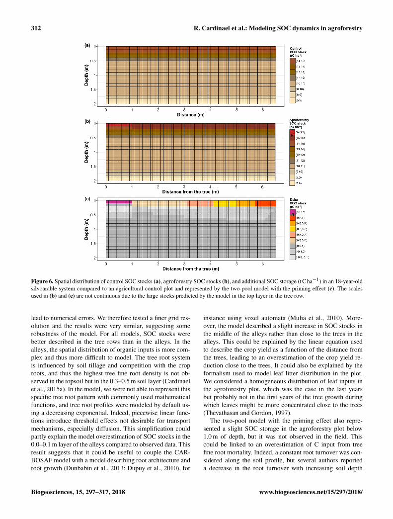
As a reminder, the SOC stocks of the agroforestry plotwere not part of the model calibration (that used the con-trol plot only) but were used here for validation. ObservedSOC stocks were not well represented by the two-poolmodel without the priming effect, with RMSE ranging from1.00 to 1.07 kgCm−3 (Fig. 5, Table S3 in the Supple-ment). The model performed better when the priming effectwas taken into account, with RMSE ranging from 0.41 to0.95 kgCm−3, and the SOC profile was well described. Therepresentation of SOC stocks was not improved by the in-clusion of a third C pool in the model. Overall, the two-poolmodel with the priming effect was the best one, as shown bythe BICs (Fig. 5, Table S3 in the Supplement). For all mod-els, SOC stocks below 1 m of depth were better describedthan SOC stocks above 1 m (Table S3 in the Supplement).The spatial distribution of SOC stocks and additional SOCstorage was also well described (Fig. 6), with very high addi-tional SOC storage in the topsoil layer in the tree row. Mostmodeled SOC storage in the agroforestry plot was located inthe first 0.2 m of depth, but SOC storage was slightly higherin the middle of the alleys than in the alleys close to the treerows.



Figure 4. Measured soil organic carbon stocks and organic carbon inputs to the soil (a) in the agricultural control plot and (b) in the 18-year-old agroforestry plot. Associated errors are standard errors. Values are expressed per hectare of land type (control, alley, tree row). To get thevalues per hectare of agroforestry, data from the alley and tree row have to be weighted by their respective surface area (i.e., 84 and 16 %,respectively) and then added up. OC: organic carbon; SOC: soil organic carbon. SOC stock data are from Cardinael et al. (2015b), and datafor tree root OC inputs are combined from Cardinael et al. (2015a) and Germon et al. (2016).



Table 5. Summary of optimized model parameters.

Model Meaning Starting Posterior values± variance (starting parameter values)parameter parameter

range

Two pools – without PE Two pools – with PE Three pools – without PE

a Coefficient from Eq. (8) of theHSOC decomposition (yr−1)

3.65e–6–3.65 0.01e−2±< 10−4 (0.01e−2) 0.01e−2

±< 10−4 (0.01e−2) –

a1 Coefficient from Eq. (8) of theHSOC1 decomposition (yr−1)

3.65e–6–3.65 – – 0.01e−2±< 10−4 (0.01e−2)

a2 Coefficient from Eq. (8) of theHSOC2 decomposition (yr−1)

3.65e–6–3.65 – – 0.83e−2± 0.17e−2 (0.83e−2)

D Diffusion coefficient (cm2 yr−1) 1e–6–1 4.62e−4±5.95e−4 (9.64e−4) 5.63e−4

± 1.42e−4 (9.01e−4) 5.24e−4±7.62e−4 (9.64e−4)

A Advection rate (mmyr−1) 1e–6–1 21.25e−4± 5.02e−4 (8.54e−4) 6.63e−4

±2.38e−4 (4.27e−4) 21.60e−4±2.24e−4 (8.54e−4)

h Humification yield 0.01–1 0.32±< 10−4 (0.34) 0.25± 1.00e−4 (0.13) 0.34± 0.03 (0.34)PE Priming coefficient 0.1–160 – 9.66± 1.49 (102.95) –f1 Fraction of decomposed FOC

entering the HSOC1 pool0–1 – – 0.99± 0.18 (0.86)

f2 Fraction of decomposed HSOC1entering the FOC pool

0–1 – – 0.94± 1.10e−3 (0.80)

The starting parameter range represents the range in which starting parameter values were sampled for the 30 optimizations per model variant. The starting parameter values presented in brackets in the posterior columnrepresent the starting parameter values that minimized the J(x) value (Eq. 34).

4 Discussion

4.1 OC inputs drive SOC storage in agroforestrysystems

Increased SOC stocks in the agroforestry plot compared tothe control may be explained by increased OC inputs, de-creased OC outputs by SOC mineralization, or both. In thealleys, higher SOC stocks in the topsoil could be explainedby inputs from litterfall and tree roots despite a decrease incrop inputs. Most of the additional SOC storage in the agro-forestry plot was found in the topsoil in the tree rows. Thesame distribution was observed for OC inputs to the soil. In-puts from the herbaceous vegetation had an important im-pact on SOC storage. The increased SOC stocks in the treerows were largely explained by an important abovegroundcarbon input (2.13 t Cha−1 yr−1) by the herbaceous vegeta-tion between trees. This result had already been suggestedby Cardinael et al. (2015b) and Cardinael et al. (2017), whoshowed that even young agroforestry systems can store SOCin the tree rows while trees are still very small. These “grassstrips” indirectly introduced by the tree planting in paralleltree rows have a major impact on the SOC stocks of agro-forestry systems. Increased SOC stocks below the ploughlayer could be explained by higher root inputs, but these in-puts could also have contributed to decreasing SOC stocksbelow 1.5 m due to the priming effect. On the plot scale,measured organic carbon inputs to the soil were increasedby 40 % (+1.1 tC ha−1 yr−1) down to 2 m of depth in the18-year-old agroforestry plot compared to the control plot,resulting in increased SOC stocks of 3.3 tCha−1. IncreasedOC inputs in agroforestry systems have been shown in otherstudies, but they were only quantified in the first 20 cm of soil(Oelbermann et al., 2006; Peichl et al., 2006). This study istherefore the first to also quantify deep OC inputs to soil.

In this study and due to a lack of data, soil temperatureand soil moisture were considered the same in both plotsso that the abiotic factors controlling SOC decompositionwere identical. Reduced soil temperature is often observedin agroforestry systems (Clinch et al., 2009; Dubbert et al.,2014), but the effect of agroforestry on soil moisture is muchmore complex. Soil evaporation is reduced under the trees,but soil water is also lost through the transpiration of trees(Ilstedt et al., 2016; Ong and Leakey, 1999). These oppos-ing effects vary with distance from the tree (Odhiambo et al.,2001). Moreover, increased water infiltration and water stor-age has been observed under the trees after a rainy event (An-derson et al., 2009). Therefore, the effect of agroforestry onsoil moisture is variable in time and space and should be in-vestigated in more detail. Interactions between soil temper-ature and soil moisture in SOC decomposition are known tobe complex (Conant et al., 2011; Moyano et al., 2013; Sierraet al., 2015). A sensitivity analysis performed on these twoboundary conditions showed that the model was not very sen-sitive to soil temperature and soil moisture (Fig. S3), but thereal effect of these two parameters on SOC dynamics un-der agroforestry systems should be specifically investigatedin future studies. Despite these simplifying assumptions onsimilarities in microclimate but also on vertical transport be-tween the control and the agroforestry system, the model cal-ibrated to the control plot was able to reproduce SOC stocksin tree rows and alleys and their depth distribution well. Thisstrong validation also revealed that OC inputs were sufficientto explain the differences in SOC stocks at this site. Further-more, the SOC decomposition rate could also be modifieddue to an absence of soil tillage in the tree rows (Balesdentet al., 1990) or to an increased aggregate stability (Udawattaet al., 2008) in the topsoil.



Figure 5. Measured and modeled soil organic carbon contents (kgCm−3) in an agricultural control plot and in an 18-year-old silvoarablesystem with a two-pool model without the priming effect (no PE), with a two-pool model with the priming effect (PE), and with a three-poolmodel without PE. Gray shaded bands represent SDs of measured SOC stocks (n= 93 in the control, n= 40 in the tree rows, and n= 60 inthe alleys).

4.2 Representation of SOC spatial heterogeneity inagroforestry systems

The lateral spatial heterogeneity of SOC stocks in the agro-forestry plot was well described by the two-pool model in-cluding the priming effect, with higher SOC stocks in thetree row topsoil than in the alleys. The model treated the car-

bon from the tree row herbaceous litter as an input to theupper layer of the mineral soil, in the same way as inputsby roots. The introduction of nitrogen in the model couldbe further tested in order to take into account a lower car-bon use efficiency due to a lack of nutrients for microbialgrowth in this litter. The strong SOC gradient observed inthe topsoil in tree rows compared to the resolution used could



Figure 6. Spatial distribution of control SOC stocks (a), agroforestry SOC stocks (b), and additional SOC storage (tCha−1) in an 18-year-oldsilvoarable system compared to an agricultural control plot and represented by the two-pool model with the priming effect (c). The scalesused in (b) and (c) are not continuous due to the large stocks predicted by the model in the top layer in the tree row.

lead to numerical errors. We therefore tested a finer grid res-olution and the results were very similar, suggesting somerobustness of the model. For all models, SOC stocks werebetter described in the tree rows than in the alleys. In thealleys, the spatial distribution of organic inputs is more com-plex and thus more difficult to model. The tree root systemis influenced by soil tillage and competition with the croproots, and thus the highest tree fine root density is not ob-served in the topsoil but in the 0.3–0.5 m soil layer (Cardinaelet al., 2015a). In the model, we were not able to represent thisspecific tree root pattern with commonly used mathematicalfunctions, and tree root profiles were modeled by default us-ing a decreasing exponential. Indeed, piecewise linear func-tions introduce threshold effects not desirable for transportmechanisms, especially diffusion. This simplification couldpartly explain the model overestimation of SOC stocks in the0.0–0.1 m layer of the alleys compared to observed data. Thisresult suggests that it could be useful to couple the CAR-BOSAF model with a model describing root architecture androot growth (Dunbabin et al., 2013; Dupuy et al., 2010), for

instance using voxel automata (Mulia et al., 2010). More-over, the model described a slight increase in SOC stocks inthe middle of the alleys rather than close to the trees in thealleys. This could be explained by the linear equation usedto describe the crop yield as a function of the distance fromthe trees, leading to an overestimation of the crop yield re-duction close to the trees. It could also be explained by theformalism used to model leaf litter distribution in the plot.We considered a homogeneous distribution of leaf inputs inthe agroforestry plot, which was the case in the last yearsbut probably not in the first years of the tree growth duringwhich leaves might be more concentrated close to the trees(Thevathasan and Gordon, 1997).

The two-pool model with the priming effect also repre-sented a slight SOC storage in the agroforestry plot below1.0 m of depth, but it was not observed in the field. Thiscould be linked to an overestimation of C input from treefine root mortality. Indeed, a constant root turnover was con-sidered along the soil profile, but several authors reporteda decrease in the root turnover with increasing soil depth



(Germon et al., 2016; Hendrick and Pregitzer, 1996; Joslinet al., 2006). However, the sensitivity analysis showed thatthe model was not sensitive to this parameter (Fig. S3 in theSupplement).

4.3 Vertical representation of SOC profiles in models

The best model to represent SOC profiles considered thepriming effect. This process can act in two different wayson the shape of SOC profiles. It has a direct effect on SOCmineralization and therefore modulates the amount of SOCin each soil layer, creating different SOC gradients. This in-directly affects the mechanisms of C transport within the soilprofile, as shown by a modification of transport coefficientsin the case of the priming effect (Table 5). Contrary to whatwas shown by Cardinael et al. (2015c) in long-term bare fal-lows receiving contrasted organic amendments, the additionof another SOC pool could not surpass the inclusion of thepriming effect in terms of model performance. Together withWutzler and Reichstein (2013) and Guenet et al. (2016), thisstudy therefore suggests that implementing the priming ef-fect into SOC models would improve model performances,especially when modeling deep SOC profiles.

We considered here the same transport coefficients for theFOC and HSOC pools, but the quality and the size of OCparticles are different, potentially leading to various move-ments in the soil by water fluxes or fauna activity (Lavelle,1997). Moreover, we considered identical transport parame-ters in the agroforestry and in the control plot, but the pres-ence of trees could modify soil structure, soil water fluxes(Anderson et al., 2009), and fauna activity (Price and Gor-don, 1999). However, the model was not very sensitive tothese parameters (Fig. S3). Further study could investigatethe role of different transport coefficients in the descriptionof SOC profiles.

4.4 Higher OC inputs or a different quality of OC?

The introduction of trees in an agricultural field not onlymodifies the amount of litter residues, but also their quality.Tree leaves, tree roots, and the herbaceous vegetation fromthe tree row have different C : N ratios, lignin, and cellulosecontents than the crop residues. Recent studies showed thatplant diversity had a positive impact on SOC storage (Langeet al., 2015; Steinbeiss et al., 2008). One of the hypothesesproposed by the authors is that diverse plant communitiesresult in more active, more abundant, and more diverse mi-crobial communities, increasing microbial products that canpotentially be stabilized. In our model, litter quality is notrelated to different SOC pools but is implicitly taken into ac-count in the FOC decomposition rate, which is weighted bythe respective contribution from the different types of OC in-puts. To test this, we performed a model run considering thatall OC inputs in the agroforestry plot were crop inputs (allFOC decomposition rates equaled the wheat decomposition

rate), but the results were not significantly different from theone presented here. Hence, we considered that changes inlitter quality in the agroforestry plot did not significantly in-fluence SOC decomposition rates.

4.5 Possible limitation of SOC storage by the primingeffect

Our modeling results suggested that the priming effect couldconsiderably reduce the capacity of soils to store organic car-bon. Our study showed that the increase in SOC stocks wasnot proportional to OC inputs, especially at depth. This re-sult has often been observed in Free-Air CO2 Enrichment(FACE) experiments. In these experiments, productivity isusually increased due to CO2 fertilization, but several au-thors also reported an increase in SOC decomposition notlinearly linked to the productivity increase (van Groenigenet al., 2014; Sulman et al., 2014). In a long-term FACE ex-periment, Carney et al. (2007) also found that SOC decreaseddue to the priming effect, offsetting 52 % of additional car-bon accumulated in aboveground and coarse root biomass.The priming effect intensity also relies on nutrient availabil-ity (Zhang et al., 2013). In agroforestry systems, tree rootscan intercept leached nitrate below the crop rooting zone(Andrianarisoa et al., 2016), reducing nutrient availability.This beneficial ecosystem service could indirectly increasethe priming effect intensity in deep soil layers.

The formalism used here to simulate the priming effect as-sumes that there is no mineralization of SOC in the absenceof fresh OC inputs (no basal respiration). This is a strong hy-pothesis, but this situation never occurs since the FOC poolis never empty (data not shown). In the alleys and below themaximum rooting depth of crops, there are no direct inputs ofFOC, but OC is transported in these deep layers due to trans-port mechanisms. However, further studies could explore theimpact of the priming effect formalism on the estimation ofits intensity by using explicit microbial biomass, for instance(Blagodatsky et al., 2010; Perveen et al., 2014).

Finally, root exudates were not quantified in this study.Several authors showed that they could induce strong prim-ing effects (Bengtson et al., 2012; Keiluweit et al., 2015),but root exudates are also a source of labile carbon, poten-tially contributing to stable SOC (Cotrufo et al., 2013). Theseopposing effects of root exudates on SOC should be furtherinvestigated, especially concerning the deep roots in agro-forestry systems.

5 Conclusions

We proposed the first model that simulates soil organic car-bon dynamics in agroforestry accounting for both the wholesoil profile and the lateral spatial heterogeneity in agro-forestry plots. The two-pool model with the priming effectdescribed reasonably well the measured SOC stocks after



18 years of agroforestry and SOC distributions with depth.It showed that the increased inputs of fresh biomass to soilin the agroforestry system explained the observed additionalSOC storage and suggested the priming effect as a processcontrolling SOC stocks in the presence of trees. This studypoints out processes that may be modified by deep-rootedtrees and deserve further study given their potential effectson SOC dynamics, such as additional inputs of C as rootexudates or altered soil structure leading to modified SOCtransport rates.

Information about the Supplement

The Supplement includes the walnut tree fine root biomass(Table S1 in the Supplement), the covariance matrices Pb ofoptimized parameters (Table S2 in the Supplement), the dif-ferent model performances (Table S3 in the Supplement), thepotential SOC decomposition rate as a function of soil depth(Fig. S1 in the Supplement), the correlation matrices of op-timized parameters (Fig. S2 in the Supplement), and a sensi-tivity analysis of the model (Fig. S3 in the Supplement).

Data availability. The data and the model are freely availableupon request and can be obtained by contacting the author([email protected]).

The Supplement related to this article is available onlineat https://doi.org/10.5194/bg-15-297-2018-supplement.

Competing interests. The authors declare that they have no conflictof interest.

Acknowledgements. This study was financed by the French Envi-ronment and Energy Management Agency (ADEME), followinga call for proposals as part of the REACCTIF program (Research onClimate Change Mitigation in Agriculture and Forestry). This workwas part of the funded project AGRIPSOL (Agroforestry for SoilProtection; 1260C0042) coordinated by Agroof. Rémi Cardinaelwas supported both by ADEME and by La Fondation de France.We thank the farmer, Mr. Breton, who allowed us to sample in hisfield. We are very grateful to our colleagues for their work in thefield since the tree planting, especially Jean-François Bourdoncle,Myriam Dauzat, Lydie Dufour, Jonathan Mineau, Alain Sellier,and Benoit Suard. We thank the colleagues and students whohelped us with measurements in the field or in the laboratory,especially Daniel Billiou, Cyril Girardin, Patricia Mahafaka, AgnèsMartin, Valérie Pouteau, Alexandre Rosa, and Manon Villeneuve.Finally, we would like to thank Jérôme Balesdent, Pierre Barré, andPhilippe Peylin for their valuable comments on the modeling partof this work.

Edited by: Andreas IbromReviewed by: Thomas Wutzler and one anonymous referee

References

Ahrens, B., Braakhekke, M. C., Guggenberger, G., Schrumpf, M.,and Reichstein, M.: Contribution of sorption, DOC transportand microbial interactions to the 14C age of a soil organic car-bon profile: Insights from a calibrated process model, Soil Biol.Biochem., 88, 390–402, 2015.

Albrecht, A. and Kandji, S. T.: Carbon sequestration in tropicalagroforestry systems, Agr. Ecosyst. Environ., 99, 15–27, 2003.

Anderson, S. H., Udawatta, R. P., Seobi, T., and Garrett, H. E.: Soilwater content and infiltration in agroforestry buffer strips, Agro-forest. Syst., 75, 5–16, 2009.

Andrianarisoa, K., Dufour, L., Bienaime, S., Zeller, B., andDupraz, C.: The introduction of hybrid walnut trees (Juglans ni-gra× regia cv. NG23) into cropland reduces soil mineral N con-tent in autumn in southern France, Agroforest. Syst., 90, 193–205, 2016.

Baisden, W. T. and Parfitt, R. L.: Bomb 14C enrichment indicatesdecadal C pool in deep soil?, Biogeochemistry, 85, 59–68, 2007.

Baisden, W. T., Amundson, R., Brenner, D. L., Cook, A. C.,Kendall, C., and Harden, J. W.: A multiisotope C and N modelinganalysis of soil organic matter turnover and transport as a func-tion of soil depth in a California annual grassland soil chronose-quence, Global Biogeochem. Cy., 16, 82-1–82-26, 2002.

Balandier, P. and Dupraz, C.: Growth of widely spaced trees. A casestudy from young agroforestry plantations in France, Agroforest.Syst., 43, 151–167, 1999.

Balesdent, J., Mariotti, A., and Boisgontier, D.: Effect of tillageon soil organic carbon mineralization estimated from 13C abun-dance in maize fields, J. Soil Sci., 41, 587–596, 1990.

Bambrick, A. D., Whalen, J. K., Bradley, R. L., Cogliastro, A., Gor-don, A. M., Olivier, A., and Thevathasan, N. V.: Spatial hetero-geneity of soil organic carbon in tree-based intercropping sys-tems in Quebec and Ontario, Canada, Agroforest. Syst., 79, 343–353, 2010.

Bengtson, P., Barker, J., and Grayston, S. J.: Evidence of a strongcoupling between root exudation, C and N availability, and stim-ulated SOM decomposition caused by rhizosphere priming ef-fects, Ecol. Evol., 2, 1843–1852, 2012.

Blagodatsky, S., Blagodatskaya, E., Yuyukina, T., andKuzyakov, Y.: Model of apparent and real priming effects:linking microbial activity with soil organic matter decomposi-tion, Soil Biol. Biochem., 42, 1275–1283, 2010.

Braakhekke, M. C., Beer, C., Hoosbeek, M. R., Reichstein, M.,Kruijt, B., Schrumpf, M., and Kabat, P.: SOMPROF: a verticallyexplicit soil organic matter model, Ecol. Model., 222, 1712–1730, 2011.

Bruun, S., Christensen, B. T., Thomsen, I. K., Jensen, E. S., andJensen, L. S.: Modeling vertical movement of organic matter ina soil incubated for 41 years with 14C labeled straw, Soil Biol.Biochem., 39, 368–371, 2007.

Burgess, P. J., Incoll, L. D., Corry, D. T., Beaton, A., and Hart, B. J.:Poplar (Populus spp.) growth and crop yields in a silvoarable ex-periment at three lowland sites in England, Agroforest. Syst., 63,157–169, 2004.


https://doi.org/10.5194/bg-15-297-2018-supplement


Cardinael, R., Mao, Z., Prieto, I., Stokes, A., Dupraz, C., Kim, J. H.,and Jourdan, C.: Competition with winter crops induces deeperrooting of walnut trees in a Mediterranean alley cropping agro-forestry system, Plant Soil, 391, 219–235, 2015a.

Cardinael, R., Chevallier, T., Barthès, B. G., Saby, N. P. A., Par-ent, T., Dupraz, C., Bernoux, M., and Chenu, C.: Impact of alleycropping agroforestry on stocks, forms and spatial distributionof soil organic carbon – a case study in a Mediterranean context,Geoderma, 259–260, 288–299, 2015b.

Cardinael, R., Eglin, T., Guenet, B., Neill, C., Houot, S., andChenu, C.: Is priming effect a significant process for long-termSOC dynamics? Analysis of a 52-years old experiment, Biogeo-chemistry, 123, 203–219, 2015c.

Cardinael, R., Chevallier, T., Cambou, A., Béral, C., Barthès, B. G.,Dupraz, C., Durand, C., Kouakoua, E., and Chenu, C.: Increasedsoil organic carbon stocks under agroforestry: a survey of sixdifferent sites in France, Agr. Ecosyst. Environ., 236, 243–255,2017.

Carney, K. M., Hungate, B. A., Drake, B. G., and Megonigal, J. P.:Altered soil microbial community at elevated CO2 leads to lossof soil carbon, P. Natl. Acad. Sci. USA, 104, 4990–4995, 2007.

Charbonnier, F., le Maire, G., Dreyer, E., Casanoves, F.,Christina, M., Dauzat, J., Eitel, J. U. H., Vaast, P., Vier-ling, L. A., and Roupsard, O.: Competition for light in hetero-geneous canopies: application of MAESTRA to a coffee (Cof-fea arabica L.) agroforestry system, Agr. Forest Meteorol., 181,152–169, 2013.

Chaudhry, A. K., Khan, G. S., Siddiqui, M. T., Akhtar, M., andAslam, Z.: Effect of arable crops on the growth of poplar (Pop-ulus deltoides) tree in agroforestry system, Pak. J. Agr. Sci., 40,82–85, 2003.

Chifflot, V., Bertoni, G., Cabanettes, A., and Gavaland, A.: Benefi-cial effects of intercropping on the growth and nitrogen status ofyoung wild cherry and hybrid walnut trees, Agroforest. Syst., 66,13–21, 2006.

Clinch, R. L., Thevathasan, N. V., Gordon, A. M., Volk, T. A., andSidders, D.: Biophysical interactions in a short rotation willowintercropping system in southern Ontario, Canada, Agr. Ecosyst.Environ., 131, 61–69, 2009.

Conant, R. T., Ryan, M. G., Ågren, G. I., Birge, H. E., David-son, E. A., Eliasson, P. E., Evans, S. E., Frey, S. D., Giar-dina, C. P., Hopkins, F. M., Hyvönen, R., Kirschbaum, M. U. F.,Lavallee, J. M., Leifeld, J., Parton, W. J., Megan Steinweg, J.,Wallenstein, M. D., Martin Wetterstedt, J. Å., and Brad-ford, M. A.: Temperature and soil organic matter decompositionrates – synthesis of current knowledge and a way forward, Glob.Change Biol., 17, 3392–3404, 2011.

Cotrufo, M. F., Wallenstein, M. D., Boot, C. M., Denef, K., andPaul, E.: The Microbial Efficiency-Matrix Stabilization (MEMS)framework integrates plant litter decomposition with soil organicmatter stabilization: do labile plant inputs form stable soil or-ganic matter?, Glob. Change Biol., 19, 988–95, 2013.

Davidson, E. A. and Janssens, I. A.: Temperature sensitivity of soilcarbon decomposition and feedbacks to climate change, Nature,440, 165–173, 2006.

Dimassi, B., Cohan, J.-P., Labreuche, J., and Mary, B.: Changes insoil carbon and nitrogen following tillage conversion in a long-term experiment in Northern France, Agr. Ecosyst. Environ., 169,12–20, 2013.

Dubbert, M., Mosena, A., Piayda, A., Cuntz, M., Correia, A. C.,Pereira, J. S., and Werner, C.: Influence of tree cover on herba-ceous layer development and carbon and water fluxes in a Por-tuguese cork-oak woodland, Acta Oecol., 59, 35–45, 2014.

Dufour, L., Metay, A., Talbot, G., and Dupraz, C.: Assessing lightcompetition for cereal production in temperate agroforestry sys-tems using experimentation and crop modelling, J. Agron. CropSci., 199, 217–227, 2013.

Dunbabin, V. M., Postma, J. A., Schnepf, A., Pagès, L., Javaux, M.,Wu, L., Leitner, D., Chen, Y. L., Rengel, Z., and Diggle, A. J.:Modelling root-soil interactions using three-dimensional modelsof root growth, architecture and function, Plant Soil, 372, 93–124, 2013.

Dupuy, L., Gregory, P. J., and Bengough, A. G.: Root growth mod-els: towards a new generation of continuous approaches, J. Exp.Bot., 61, 2131–2143, 2010.

Duursma, R. A. and Medlyn, B. E.: MAESPA: a model to studyinteractions between water limitation, environmental drivers andvegetation function at tree and stand levels, with an example ap-plication to [CO2] × drought interactions, Geosci. Model Dev.,5, 919–940, https://doi.org/10.5194/gmd-5-919-2012, 2012.

Eilers, K. G., Debenport, S., Anderson, S., and Fierer, N.: Diggingdeeper to find unique microbial communities: The strong effectof depth on the structure of bacterial and archaeal communitiesin soil, Soil Biol. Biochem., 50, 58–65, 2012.

Eissenstat, D. M. and Yanai, R. D.: The ecology of root lifespan,Adv. Ecol. Res., 27, 1–60, 1997.

Ellert, B. H. and Bettany, J. R.: Calculation of organic matter andnutrients stored in soils under contrasting management regimes,Can. J. Soil Sci., 75, 529–538, 1995.

Elzein, A. and Balesdent, J.: Mechanistic simulation of vertical dis-tribution of carbon concentrations and residence times in soils,Soil Sci. Soc. Am. J., 59, 1328–1335, 1995.

Fierer, N., Schimel, J. P., and Holden, P. A.: Variations in micro-bial community composition through two soil depth profiles, SoilBiol. Biochem., 35, 167–176, 2003.

Fontaine, S., Barot, S., Barré, P., Bdioui, N., Mary, B., andRumpel, C.: Stability of organic carbon in deep soil layers con-trolled by fresh carbon supply, Nature, 450, 277–281, 2007.

Germon, A., Cardinael, R., Prieto, I., Mao, Z., Kim, J. H.,Stokes, A., Dupraz, C., Laclau, J.-P., and Jourdan, C.: Unex-pected phenology and lifespan of shallow and deep fine roots ofwalnut trees grown in a silvoarable Mediterranean agroforestrysystem, Plant Soil, 401, 409–426, 2016.

Graves, A. R., Burgess, P. J., Palma, J. H. N., Herzog, F.,Moreno, G., Bertomeu, M., Dupraz, C., Liagre, F., Keesman, K.,van der Werf, W., de Nooy, a. K., and van den Briel, J. P.: Devel-opment and application of bio-economic modelling to comparesilvoarable, arable, and forestry systems in three European coun-tries, Ecol. Eng., 29, 434–449, 2007.

Graves, A. R., Burgess, P. J., Palma, J., Keesman, K. J., vander Werf, W., Dupraz, C., van Keulen, H., Herzog, F., andMayus, M.: Implementation and calibration of the parameter-sparse Yield-SAFE model to predict production and land equiv-alent ratio in mixed tree and crop systems under two contrastingproduction situations in Europe, Ecol. Model., 221, 1744–1756,2010.

Guenet, B., Eglin, T., Vasilyeva, N., Peylin, P., Ciais, P., andChenu, C.: The relative importance of decomposition and trans-


https://doi.org/10.5194/gmd-5-919-2012


port mechanisms in accounting for soil organic carbon profiles,Biogeosciences, 10, 2379–2392, https://doi.org/10.5194/bg-10-2379-2013, 2013.

Guenet, B., Moyano, F. E., Peylin, P., Ciais, P., and Janssens,I. A.: Towards a representation of priming on soil car-bon decomposition in the global land biosphere model OR-CHIDEE (version 1.9.5.2), Geosci. Model Dev., 9, 841–855,https://doi.org/10.5194/gmd-9-841-2016, 2016.

Haile, S. G., Nair, V. D., and Nair, P. K. R.: Contribution of trees tocarbon storage in soils of silvopastoral systems in Florida, USA,Glob. Change Biol., 16, 427–438, 2010.

Hendrick, R. L. and Pregitzer, K. S.: Temporal and depth-relatedpatterns of fine root dynamics in northern hardwood forests, J.Ecol., 84, 167–176, 1996.

Howlett, D. S., Moreno, G., Mosquera Losada, M. R., Nair, P. K. R.,and Nair, V. D.: Soil carbon storage as influenced by tree coverin the Dehesa cork oak silvopasture of central-western Spain, J.Environ. Monitor., 13, 1897–904, 2011.

Ilstedt, U., Bargués Tobella, A., Bazié, H. R., Bayala, J., Ver-beeten, E., Nyberg, G., Sanou, J., Benegas, L., Murdiyarso, D.,Laudon, H., Sheil, D., and Malmer, A.: Intermediate tree covercan maximize groundwater recharge in the seasonally dry trop-ics, Sci. Rep.-UK, 6, 1–12, https://doi.org/10.1038/srep21930,2016.

IUSS Working Group WRB: World Reference Base for Soil Re-sources 2006, first update 2007. World Soil Resources ReportsNo. 103, FAO, Rome, 2007.

Jobbagy, E. G. and Jackson, R. B.: The vertical distribution of soilorganic carbon and its relation to climate and vegetation, Ecol.Appl., 10, 423–436, 2000.

Joslin, J. D., Gaudinski, J. B., Torn, M. S., Riley, W. J., and Han-son, P. J.: Fine-root turnover patterns and their relationship toroot diameter and soil depth in a 14C-labeled hardwood forest,New Phytol., 172, 523–535, 2006.

Kätterer, T., Bolinder, M. A., Andrén, O., Kirchmann, H., andMenichetti, L.: Roots contribute more to refractory soil organicmatter than above-ground crop residues, as revealed by a long-term field experiment, Agr. Ecosyst. Environ., 141, 184–192,2011.

Keiluweit, M., Bougoure, J. J., Nico, P. S., Pett-Ridge, J., We-ber, P. K., and Kleber, M.: Mineral protection of soil carboncounteracted by root exudates, Nat. Clim. Chang, 5, 588–595,2015.

Kim, D.-G., Kirschbaum, M. U. F., and Beedy, T. L.: Carbon se-questration and net emissions of CH4 and N2O under agro-forestry: Synthesizing available data and suggestions for futurestudies, Agr. Ecosyst. Environ., 226, 65–78, 2016.

Koarashi, J., Hockaday, W. C., Masiello, C. A., and Trumbore, S. E.:Dynamics of decadally cycling carbon in subsurface soils, J.Geophys. Res., 117, 1–13, 2012.

Koven, C. D., Riley, W. J., Subin, Z. M., Tang, J. Y., Torn, M.S., Collins, W. D., Bonan, G. B., Lawrence, D. M., and Swen-son, S. C.: The effect of vertically resolved soil biogeochemistryand alternate soil C and N models on C dynamics of CLM4,Biogeosciences, 10, 7109–7131, https://doi.org/10.5194/bg-10-7109-2013, 2013.

Lange, M., Eisenhauer, N., Sierra, C. A., Bessler, H., En-gels, C., Griffiths, R. I., Mellado-Vázquez, P. G., Malik, A. A.,Roy, J., Scheu, S., Steinbeiss, S., Thomson, B. C., Trum-

bore, S. E., and Gleixner, G.: Plant diversity increases soil mi-crobial activity and soil carbon storage, Nat. Commun., 6, 1–8,https://doi.org/10.1038/ncomms7707, 2015.

Lavelle, P.: Faunal Activities and Soil Processes: AdaptativeStrategy that Determine Ecosystem Function, Amsterdam, TheNetherlands, Elsevier, 1997.

Li, F., Meng, P., Fu, D., and Wang, B.: Light distribution, photosyn-thetic rate and yield in a Paulownia-wheat intercropping systemin China, Agroforest. Syst., 74, 163–172, 2008.

Lorenz, K. and Lal, R.: Soil organic carbon sequestration in agro-forestry systems. A review, Agron. Sustain. Dev., 34, 443–454,2014.

Luedeling, E., Smethurst, P. J., Baudron, F., Bayala, J., Huth, N. I.,van Noordwijk, M., Ong, C. K., Mulia, R., Lusiana, B.,Muthuri, C., and Sinclair, F. L.: Field-scale modeling of tree-cropinteractions: challenges and development needs, Agric. Syst.,142, 51–69, 2016.

Mead, R. and Willey, R. W.: The concept of a “land equivalent ratio”and advantages in yields from intercropping, Exp. Agr., 16, 217–228, 1980.

Moreno, G., Obrador, J. J., Cubera, E., and Dupraz, C.: Fine rootdistribution in Dehesas of central-western Spain, Plant Soil, 277,153–162, 2005.

Moyano, F. E., Vasilyeva, N., Bouckaert, L., Cook, F., Craine, J.,Curiel Yuste, J., Don, A., Epron, D., Formanek, P., Franzlueb-bers, A., Ilstedt, U., Kätterer, T., Orchard, V., Reichstein, M.,Rey, A., Ruamps, L., Subke, J.-A., Thomsen, I. K., and Chenu,C.: The moisture response of soil heterotrophic respiration: in-teraction with soil properties, Biogeosciences, 9, 1173–1182,https://doi.org/10.5194/bg-9-1173-2012, 2012.

Moyano, F. E., Manzoni, S., and Chenu, C.: Responses of soil het-erotrophic respiration to moisture availability: An exploration ofprocesses and models, Soil Biol. Biochem., 59, 72–85, 2013.

Mulia, R. and Dupraz, C.: Unusual fine root distributions of two de-ciduous tree species in southern France: What consequences formodelling of tree root dynamics?, Plant Soil, 281, 71–85, 2006.

Mulia, R., Dupraz, C., and van Noordwijk, M.: Reconciling rootplasticity and architectural ground rules in tree root growth mod-els with voxel automata, Plant Soil, 337, 77–92, 2010.

Nair, P. K.: An Introduction to Agroforestry, Kluwer AcademicPublishers, Dordrecht, The Netherlands, 1993.

Nair, P. K. R.: Classification of agroforestry systems, Agrofor. Syst.,3, 97–128, 1985.

Odhiambo, H. O., Ong, C. K., Deans, J. D., Wilson, J.,Khan, A. A. H., and Sprent, J. I.: Roots, soil water and cropyield: Tree crop interactions in a semi-arid agroforestry systemin Kenya, Plant Soil, 235, 221–233, 2001.

Oelbermann, M. and Voroney, R. P.: And evaluation of the centurymodel to predict soil organic carbon: examples from Costa Ricaand Canada, Agrofor. Syst., 82, 37–50, 2011.

Oelbermann, M., Voroney, R. P., and Gordon, A. M.: Carbon se-questration in tropical and temperate agroforestry systems: a re-view with examples from Costa Rica and southern Canada, Agr.Ecosyst. Environ., 104, 359–377, 2004.

Oelbermann, M., Voroney, R. P., Thevathasan, N. V., Gordon, A. M.,Kass, D. C. L., and Schlönvoigt, A. M.: Soil carbon dynamicsand residue stabilization in a Costa Rican and southern Canadianalley cropping system, Agroforest. Syst., 68, 27–36, 2006.


https://doi.org/10.5194/bg-10-2379-2013

https://doi.org/10.5194/bg-10-2379-2013

https://doi.org/10.5194/gmd-9-841-2016

https://doi.org/10.1038/srep21930

https://doi.org/10.5194/bg-10-7109-2013

https://doi.org/10.5194/bg-10-7109-2013

https://doi.org/10.1038/ncomms7707

https://doi.org/10.5194/bg-9-1173-2012


Ong, C. K. and Leakey, R. R. B.: Why tree-crop interactions in agro-forestry appear at odds with tree-grass interactions in tropical sa-vannahs, Agroforest. Syst., 45, 109–129, 1999.

Parton, W. J., Schimel, D. S., Cole, C. V., and Ojima, D. S.: Analysisof factors controlling soil organic matter levels in great plainsgrasslands, Soil Sci. Soc. Am. J., 51, 1173–1179, 1987.

Peichl, M., Thevathasan, N. V, Gordon, A. M., Huss, J., and Abo-hassan, R. A.: Carbon sequestration potentials in temperate tree-based intercropping systems, southern Ontario, Canada, Agro-forest. Syst., 66, 243–257, 2006.

Perveen, N., Barot, S., Alvarez, G., Klumpp, K., Martin, R., Ra-paport, A., Herfurth, D., Louault, F., and Fontaine, S.: Primingeffect and microbial diversity in ecosystem functioning and re-sponse to global change: a modeling approach using the SYM-PHONY model, Glob. Change Biol., 20, 1174–1190, 2014.

Price, G. W. and Gordon, A. M.: Spatial and temporal distributionof earthworms in a temperate intercropping system in southernOntario, Canada, Agroforest. Syst., 44, 141–149, 1999.

Prieto, I., Roumet, C., Cardinael, R., Kim, J., Maeght, J.-L.,Mao, Z., Portillo, N., Thammahacksa, C., Dupraz, C., Jour-dan, C., Pierret, A., Roupsard, O., and Stokes, A.: Rootfunctional parameters along a land-use gradient: evidence ofa community-level economics spectrum, J. Ecol., 103, 361–373,2015.

Prieto, I., Stokes, A., and Roumet, C.: Root functional parame-ters predict fine root decomposability at the community level, J.Ecol., 104, 725–733, 2016.

R Development Core Team: R: A Language and Environment forStatistical Computing, Vienna, Austria, the R Foundation for Sta-tistical Computing, 2013.

Rasse, D. P., Mulder, J., Moni, C., and Chenu, C.: Carbon turnoverkinetics with depth in a French loamy soil, Soil Sci. Soc. Am. J.,70, 2097–2105, 2006.

Salomé, C., Nunan, N., Pouteau, V., Lerch, T. Z., and Chenu, C.:Carbon dynamics in topsoil and in subsoil may be controlled bydifferent regulatory mechanisms, Glob. Change Biol., 16, 416–426, 2010.

Santaren, D., Peylin, P., Viovy, N., and Ciais, P.: Optimizinga process-based ecosystem model with eddy-covariance fluxmeasurements: a pine forest in southern France, Global Bio-geochem. Cy., 21, 1–15, 2007.

Schwarz, G.: Estimating dimension of a model, Ann. Stat., 6, 461–464, 1978.

Shahzad, T., Chenu, C., Genet, P., Barot, S., Perveen, N., Mou-gin, C., and Fontaine, S.: Contribution of exudates, arbuscularmycorrhizal fungi and litter depositions to the rhizosphere prim-ing effect induced by grassland species, Soil Biol. Biochem., 80,146–155, 2015.

Sierra, C. A., Trumbore, S. E., Davidson, E. A., Vicca, S., andJanssens, I.: Sensitivity of decomposition rates of soil organicmatter with respect to simultaneous changes in temperature andmoisture, J. Adv. Model. Earth Sy., 7, 335–356, 2015.

Soetaert, K., Petzoldt, T., and Woodrow Setzer, R.: Solving differ-ential equations in R: package deSolve, J. Stat. Softw., 33, 1–25,2010.

Somarriba, E.: Revisiting the past: an essay on agroforestry defini-tion, Agroforest. Syst., 19, 233–240, 1992.

Steinbeiss, S., Beßler, H., Engels, C., Temperton, V. M., Buch-mann, N., Roscher, C., Kreutziger, Y., Baade, J., Habekost, M.,

and Gleixner, G.: Plant diversity positively affects short-term soilcarbon storage in experimental grasslands, Glob. Change Biol.,14, 2937–2949, 2008.

Sulman, B. N., Phillips, R. P., Oishi, A. C., Shevliakova, E., andPacala, S. W.: Microbe-driven turnover offsets mineral-mediatedstorage of soil carbon under elevated CO2, Nat. Clim. Change, 4,1099–1102, 2014.

Taghizadeh-Toosi, A., Christensen, B. T., Hutchings, N. J., Ve-jlin, J., Kätterer, T., Glendining, M., and Olesen, J. E.: C-TOOL:a simple model for simulating whole-profile carbon storage intemperate agricultural soils, Ecol. Model., 292, 11–25, 2014.

Talbot, G.: L’intégration spatiale et temporelle du partage desressources dans un système agroforestier noyers-céréales: uneclef pour en comprendre la productivité?, PhD Dissertation, Uni-versité Montpellier II, Montpellier, France, 2011.

Tarantola, A.: Inverse Problem Theory: Methods for Data Fit-ting and Model Parameter Estimation, Elsevier, the Netherlands,1987.

Tarantola, A.: Inverse Problem Theory and Methods for Model Pa-rameter Estimation, SIAM, Philadelphia, USA, 2005.

Thevathasan, N. V. and Gordon, A. M.: Poplar leaf biomass dis-tribution and nitrogen dynamics in a poplar-barley intercroppedsystem in southern Ontario, Canada, Agroforest. Syst., 37, 79–90, 1997.

Udawatta, R. P., Kremer, R. J., Adamson, B. W., and Ander-son, S. H.: Variations in soil aggregate stability and enzyme ac-tivities in a temperate agroforestry practice, Appl. Soil Ecol., 39,153–160, 2008.

van der Werf, W., Keesman, K., Burgess, P., Graves, A., Pil-beam, D., Incoll, L. D., Metselaar, K., Mayus, M., Stap-pers, R., van Keulen, H., Palma, J., and Dupraz, C.: Yield-SAFE:A parameter-sparse, process-based dynamic model for predict-ing resource capture, growth, and production in agroforestry sys-tems, Ecol. Eng., 29, 419–433, 2007.

van Groenigen, K. J., Qi, X., Osenberg, C. W., Luo, Y., and Hun-gate, B. A.: Faster decomposition under increased atmosphericCO2 limits soil carbon storage, Science, 344, 508–509, 2014.

van Noordwijk, M. and Lusiana, B.: WaNuLCAS, a model of water,nutrient and light capture in agroforestry systems, Agrofor. Syst.,43, 217–242, 1999.

Virto, I., Barré, P., Burlot, A., and Chenu, C.: Carbon input differ-ences as the main factor explaining the variability in soil organicC storage in no-tilled compared to inversion tilled agrosystems,Biogeochemistry, 108, 17–26, 2012.

Wutzler, T. and Reichstein, M.: Colimitation of decomposition bysubstrate and decomposers – a comparison of model formula-tions, Biogeosciences, 5, 749–759, https://doi.org/10.5194/bg-5-749-2008, 2008.

Wutzler, T. and Reichstein, M.: Priming and substrate quality inter-actions in soil organic matter models, Biogeosciences, 10, 2089–2103, https://doi.org/10.5194/bg-10-2089-2013, 2013.

Yin, R. and He, Q.: The spatial and temporal effects of paulowniaintercropping: the case of northern China, Agroforest. Syst., 37,91–109, 1997.

Zhang, W., Wang, X., and Wang, S.: Addition of ex-ternal organic carbon and native soil organic carbondecomposition: a meta-analysis, PLoS One, 8, 1–6,https://doi.org/10.1371/journal.pone.0054779, 2013.


https://doi.org/10.5194/bg-5-749-2008

https://doi.org/10.5194/bg-5-749-2008

https://doi.org/10.5194/bg-10-2089-2013

https://doi.org/10.1371/journal.pone.0054779

Documents

High organic inputs explain shallow and deep SOC storage