INSTITUTE OF PHYSICS PUBLISHING NONLINEARITY

Nonlinearity 19 (2006) 2581–2603 doi:10.1088/0951-7715/19/11/005

High-order surface relaxation versus theEhrlich–Schwoebel effect

Bo Li

Department of Mathematics, University of California, San Diego, 9500 Gilman Drive,Mail code: 0112, La Jolla, CA 92093-0112, USA

E-mail: bli@math.ucsd.edu

Received 2 February 2006, in final form 8 September 2006Published 28 September 2006Online at stacks.iop.org/Non/19/2581

Recommended by C Le Bris

AbstractWe consider a class of continuum models of epitaxial growth of thin films withtwo competing mechanisms: (1) the surface relaxation described by high-ordergradients of the surface profile and (2) the Ehrlich–Schwoebel (ES) effect whichis the asymmetry in the adatom attachment and detachment to and from atomicsteps. Mathematically, these models are gradient-flows of some effective free-energy functionals for which large slopes are preferred for surfaces with lowenergy.

We characterize the large-system asymptotics of the minimum energy andthe magnitude of gradients of energy-minimizing surfaces. We also show that,in the large-system limit, the renormalized energy with an infinite ES barrieris the �-limit of those with a finite one, indicating the enhancement of theES effect in a large system. Introducing λ-minimizers as energy minimizersamong all candidates that are spatially λ-periodical, we show the existence ofa sequence of such λ-minimizers that are in fact equilibriums. For the case ofa finite ES effect, we prove the well-posedness of the initial-boundary-valueproblem of the continuum model and obtain bounds for the scaling laws ofinterface width, surface slope and energy, all of which characterize the surfacecoarsening during the film growth. We conclude with a discussion on theimplications of our rigorous analysis.

Mathematics Subject Classification: 34K26, 49J45, 74G65, 74K30

PACS numbers: 68.35.Ct; 68.43.Jk; 81.15.Aa

0951-7715/06/112581+23$30.00 © 2006 IOP Publishing Ltd and London Mathematical Society Printed in the UK 2581

2582 B Li

1. Introduction

In the form of mass balance, a continuum model of epitaxial growth of thin films is given by

∂th + ∇ · j = F, (1.1)

where h = h(x, t) with x = (x1, x2) is the coarse-grained height profile of the film surfaceat time t , j = j(∇h, ∇2h, . . .) is the surface current or flux which depends only on gradientsof h but not explicitly on x due to the translational invariance in h and x, and F is the meandeposition flux which we assume to be a positive constant [4, 24]. Here, we neglect the noisein the deposition flux.

The current j describes microscopic processes in the growth that determine macroscopicproperties of films and growth scaling laws. It can include many different processes andmechanisms. In this work, we consider two such important processes and mechanisms thatcompete with each other.

The first one is a high-order surface relaxation, i.e. surface relaxation described by high-order gradients of the height profile h. This process smoothens the surface in general.

The current due to such relaxation is given by

jRE = (−1)mMm∇�m−1h, (1.2)

where m � 2 is an integer, Mm the mobility which is taken to be a positive constant here, ∇the gradient and � the Laplacian. Here, we assume that the surface current is isotropic—oftenan idealized situation in the growth of a crystalline surface.

For m = 2, the current (1.2) is the Herring–Mullins term for the isotropic surfacediffusion [11, 23]. It can be derived for some cases from a Burton–Cabrera–Frank (BCF)type model [6, 17, 22]. The surface relaxation with m = 3 in (1.2), together with lower-orderterms, has been suggested to model the homoepitaxy of Fe(001) at room temperature [33].The physical origin of the relaxation with m � 3 remains unclear and a satisfactory derivationof such a term seems to be challenging.

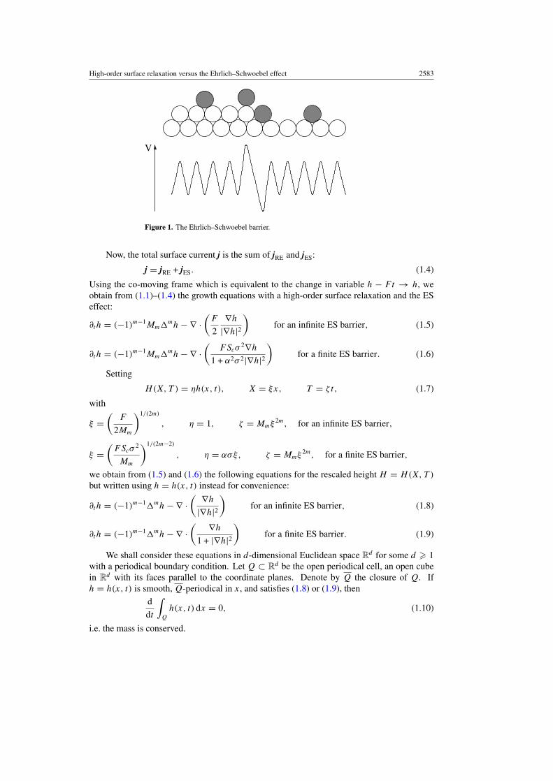
The second one is the adatom (adsorbed atom) attachment–detachment with the Ehrlich–Schwoebel (ES) effect: in order to stick to an atomic step, an adatom from an upper terracemust overcome an energy barrier—the ES barrier—in addition to the diffusion barrier on anatomistically flat terrace [7, 29, 30]; cf figure 1.

The ES effect generates an uphill current that destabilizes nominal surfaces (high-symmetry surfaces) but stabilizes vicinal surfaces (stepped surfaces that are in the vicinityof high-symmetry surfaces) with a large slope, preventing step bunching [7, 30, 36]. This isthe origin of the Bales–Zangwill instability, a diffusional instability of atomic steps [3]. It alsoaffects the island nucleation [16]. With the ES effect, the film surface prefers a large slope.The competition between this large-slope preference and the surface relaxation determines thelarge-scale surface morphology and growth scaling laws [2, 10, 12, 20, 25, 27, 31, 36].

The exact form of the current induced by an infinite ES barrier was first proposed in [36]and that by a finite ES barrier in [12]; see also [15, 26, 31]. These forms are

jES =

F

2

∇h

|∇h|2 for an infinite ES barrier,

FScσ2∇h

1 + α2σ 2|∇h|2 for a finite ES barrier,

(1.3)

where Sc > 0 is a constant measuring the strength of the ES effect, σ > 0 the nucleation lengthand α > 0 an interpolation constant—a fitting parameter [12]. For the case of an infinite ESbarrier, the current is also given in [12] in a slightly altered form (without the factor 1/2).

High-order surface relaxation versus the Ehrlich–Schwoebel effect 2583

V

Figure 1. The Ehrlich–Schwoebel barrier.

Now, the total surface current j is the sum of jRE and jES:

j = jRE + jES. (1.4)

Using the co-moving frame which is equivalent to the change in variable h − F t → h, weobtain from (1.1)–(1.4) the growth equations with a high-order surface relaxation and the ESeffect:

∂th = (−1)m−1Mm�mh − ∇ ·(

F

2

∇h

|∇h|2)

for an infinite ES barrier, (1.5)

∂th = (−1)m−1Mm�mh − ∇ ·(

FScσ2∇h

1 + α2σ 2|∇h|2)

for a finite ES barrier. (1.6)

Setting

H(X, T ) = ηh(x, t), X = ξx, T = ζ t, (1.7)

with

ξ =(

F

2Mm

)1/(2m)

, η = 1, ζ = Mmξ 2m, for an infinite ES barrier,

ξ =(

FScσ2

Mm

)1/(2m−2)

, η = ασξ, ζ = Mmξ 2m, for a finite ES barrier,

we obtain from (1.5) and (1.6) the following equations for the rescaled height H = H(X, T )

but written using h = h(x, t) instead for convenience:

∂th = (−1)m−1�mh − ∇ ·( ∇h

|∇h|2)

for an infinite ES barrier, (1.8)

∂th = (−1)m−1�mh − ∇ ·( ∇h

1 + |∇h|2)

for a finite ES barrier. (1.9)

We shall consider these equations in d-dimensional Euclidean space Rd for some d � 1

with a periodical boundary condition. Let Q ⊂ Rd be the open periodical cell, an open cube

in Rd with its faces parallel to the coordinate planes. Denote by Q the closure of Q. If

h = h(x, t) is smooth, Q-periodical in x, and satisfies (1.8) or (1.9), then

d

dt

∫Q

h(x, t) dx = 0, (1.10)

i.e. the mass is conserved.

2584 B Li

Let us denote for any integer k � 0 and any function u which has all the derivatives up toorder k

Wk(u) ={

|�k/2u|2 if k is even,

|∇�(k−1)/2u|2 if k is odd,(1.11)

where �0u = u. We can verify that equations (1.8) and (1.9) with the Q-periodical boundarycondition are formally the gradient flows of the following effective free-energy functionals,respectively:

I (h) = −∫

Q

[1

2Wm(h) − log |∇h|

]dx for an infinite ES barrier, (1.12)

J (h) = −∫

Q

[1

2Wm(h) − 1

2log(1 + |∇h|2)

]dx for a finite ES barrier. (1.13)

Here and below,

−∫

E

u dx = 1

|E|∫

E

u dx (1.14)

denotes the mean value of a Lebesgue integrable function u : E → R with E a d-dimensionalLebesgue measurable set with a finite Lebesgue measure |E| > 0.

It is clear by (1.12) or (1.13) that a low-energy profile should have a large slope which isbalanced by the relaxation term. The surface slope should thus increase with time during thedynamics governed by (1.8) or (1.9).

Our main results are as follows.

(1) For each of the energy functionals I and J , the infimum is attained in a suitable Sobolevspace. Moreover, if L > 0 is the linear size of the periodical cell Q, then the minimumenergy for I or J is

−(m − 1) log L + O(1) as L → ∞,

and for any energy minimizer h of I or J ,√−∫

Q

|∇kh|2 dx = O(Lm−k), k = 0, . . . , m, as L → ∞,

where ∇k represents all the derivatives of order k, cf (2.1). See theorem 2.1 andcorollary 2.1.

(2) If L is the linear size of the periodical cell Q, then there exists an L/n-minimizer ofthe energy functional I or J for each integer n � 1, and such an L/n- minimizer isin fact an equilibrium solution in the case of a finite ES barrier. Here, we define a λ-minimizer for λ > 0 to be an energy-minimizer among all admissible functions that are[0, λ]d -periodical. See definition 2.1 and theorem 2.2.

(3) As the system size increases, a new energy functional renormalized from I is the �-limitof those renormalized from J . See theorems 3.1 and 3.2.

(4) The initial-boundary-value problem of the growth equation (1.9) with a periodicalboundary condition is well-posed. See theorem 4.1.

(5) If h = h(x, t) is a smooth, Q-periodical solution of (1.9), then

wh(t) � Ct1/2,√−∫ t

t0

−∫

Q

|∇kh(x, τ )|2 dx dτ � Ct(m−k)/(2m), k = 1, . . . , m,

I (h(·, t)) � −m − 1

2mlog t + C,

High-order surface relaxation versus the Ehrlich–Schwoebel effect 2585

where wh(t) is the interface width of h (cf (5.1)) and C is a generic constant that isindependent of h, Q and t . See theorem 5.1.If h = h(x, t) is a solution of (1.6) with the given parameters Mm, F , Sc, σ and α, thenwe find that for any t0 � 0 and t > t0 large enough

wh(t) �√

2FSc

α2t + C,

√−∫ t

t0

−∫

Q

Wk(h(x, τ )) dx dτ �√

FSc

αMk/(2m)m

tm−k2m + C, k = 1, . . . , m,

where C > 0 is a constant independent of h, Q and t . See corollary 5.1.

Part (1) and Part (2) above are parallel in part to the related results in [20]. They areobtained by studying the rescaled, singularly perturbed energy functionals; cf (2.7) and (2.8).Our results here, however, are valid for any integer m � 2 and for both the functionals I andJ . These results are optimal and their proofs are much refined. Note that the term − log |∇h|in the energy functional I defined in (1.12) has to be treated with care. The concept of λ-minimizers, though first introduced here, has been used implicitly in [20,25] to predict scalinglaws for the coarsening dynamics in epitaxial growth. See more discussions in section 6.

It is important to treat the spacial case of an infinite ES barrier which is studied in [10]to obtain the scaling laws. Our �-convergence result in Part (3) indicates that the ES effect isenhanced in a large system. This is because the slope of a film surface can become large—andhence the ES instability can be fully developed—only in a large system. Consequently, afinite ES barrier can be regarded effectively as an infinite one in a large system. Some of thetechniques used in proving the results in Parts (1)–(3) are developed in our recent work [21].

The well-posedness in Part (4) provides a basis for any of the growth scaling laws to bemathematically meaningful. At this point, the well-posedness of the initial-boundary-valueproblem for the equation (1.8) is not obtained.

Finally, our bounds in Part (5) are only one-sided. Two-sided bounds can never be validfor steady-state solutions and hence for all the solutions. Our method for proving the upperbounds in Part (5) is different from that in [13, 14]. In our case, there are two independentquantities: one is the surface height and the other the lateral size of mounds (or, independently,the surface slope). Moreover, the surface slope can increase and the energy can decreaseunbounded with respect to the increase in the system size. Our argument is elementary and isbased on observations on the relation between the height profile and its gradients.

The rest of this paper is organized as follows: in section 2, we study the large-systemasymptotics as well as λ-minimizers of the energy functionals (1.12) and (1.13); in section 3,we show the�-convergence of renormalized energies; in section 4, we prove the well-posednessof the initial-boundary-value problem of equation (1.9); in section 5, we give bounds on theinterface width, gradients and energy for solutions of equation (1.9); finally, in section 6, wefurther discuss the result of our analysis.

2. Energy minimization

In this section, we study the asymptotics of ‘ground states’ and special equilibriums, theλ-minimizers. These variational properties can be used to predict scaling laws; cf section 6.

Let us fix a cube Q ⊂ Rd as above. Denote by C∞

per(Q) the set of all real-valued, Q-periodic, C∞-functions on R

d . For any integer k � 1, let Hkper(Q) be the closure in the usual

Sobolev space Hk(Q) = Wk,2(Q) of the set of all functions in C∞per(Q) restricted onto Q [1,9].

2586 B Li

As usual, we denote H 0(Q) = L2(Q). By (1.10), we can always assume that the constantmean-value of h over Q is in fact 0. Thus, we introduce

H◦ k

per(Q) ={u ∈ Hk

per(Q) :∫

Q

u dx = 0

}.

It is clear that H◦ k

per(Q) is a closed subspace of Hkper(Q).

For any integer k � 1 and any u : Q → R that has all the weak derivatives of order k, wedefine |∇ku| by

|∇ku|2 =∑|β|=k

|∂βu|2, (2.1)

where β in the sum is a d-dimensional index. As usual, |∇0u|2 = |u|2 for any function u.Note that ∇2 �= � for d � 2. By the Poincare inequality, there exist constants K1(k, Q) > 0and K2(k, Q) > 0 such that

K1(k, Q)‖u‖Hk(Q) � ‖∇ku‖L2(Q) � K2(k, Q)‖u‖Hk(Q) ∀u ∈ H◦ k

per(Q). (2.2)

By integration by parts, we have (cf lemma 3.1 in [19])∫Q

|�u|2 dx =∫

Q

|∇2u|2 dx ∀u ∈ H 2per(Q).

Thus, it follows from (1.11) and (2.2) that there exist constantsK3(k, Q) > 0 andK4(k, Q) > 0such that

K3(k, Q)‖u‖Hk(Q) �√∫

Q

Wk(u) dx � K4(k, Q)‖u‖Hk(Q) ∀u ∈ H◦ k

per(Q). (2.3)

Associated with the integral in (2.3) is the bilinear form A : Hkper(Q) × Hk

per(Q) → R,defined by

Ak(u, v) ={∫

Q�k/2u�k/2v dx if k is even∫

Q∇�(k−1)/2u · ∇�(k−1)/2v dx if k is odd

∀u, v ∈ Hkper(Q). (2.4)

Clearly,

Ak(u, u) =∫

Q

Wk(u) dx ∀u ∈ Hkper(Q). (2.5)

To study the large-system asymptotics, we need to scale the underlying domain Q in thedefinition of the functionals I and J (cf (1.12) and (1.13)) to a fixed domain. Thus, assumingQ = (0, L)d and setting ε = 1/L, we rescale the energy functionals (1.12) and (1.13) to get

I (h) = Iε(h) and J (h) = Jε(h) with h(x) = εh(x) and x = εx,

(2.6)

where

Iε(h) =∫

Q1

[ε2(m−1)

2Wm(h) − log |∇h|

]dx, (2.7)

Jε(h) =∫

Q1

[ε2(m−1)

2Wm(h) − 1

2log

(1 + |∇h|2)] dx, (2.8)

and Q1 = (0, 1)d is the unit cube in Rd .

High-order surface relaxation versus the Ehrlich–Schwoebel effect 2587

Throughout the rest of the paper, we fix the integers d � 1 and m � 2 and the constantL > 0. We also use the notation

Q = (0, L)d, Q1 = (0, 1)d, H(Q) = H◦ m

per(Q), H = H◦ m

per(Q1). (2.9)

The following theorem gives the optimal asymptotics of the minimum energy andmagnitude of gradients of energy minimizers for both the singularly perturbed functionals(2.7) and (2.8).

Theorem 2.1.

(1) For any ε > 0, the infimum of Iε : H → R ∪ {∞} and that of Jε : H → R are finite andattained. Moreover, for any ε ∈ (0, 1]

(m − 1) log ε + minu∈H

J1(u) � minh∈H

Jε(h) � minh∈H

Iε(h) = (m − 1) log ε + minu∈H

I1(u).

(2.10)

(2) There exist constants C1 > 0, C2 > 0 and ε0 ∈ (0, 1], all depending only on d and m,such that for any energy minimizer h ∈ H of Iε : H → R ∪ {∞} or Jε : H → R and anyε ∈ (0, ε0],

C1ε1−m � ‖∇kh‖L2(Q1) � C2ε

1−m, k = 0, . . . , m.

To prove this theorem, we recall the following result (cf lemma 3.1 in [21]) that shows thelower semicontinuity of the logarithmic part of the energy functional (2.7) and the finitenessof such energy of a limiting function.

Lemma 2.1. Let E ⊂ Rd be Lebesgue measurable with 0 < |E| < ∞. Suppose gj → g in

L1(E) and {∫E

log |gj | dx}∞j=1 is bounded. Then, log |g| ∈ L1(E) and

lim infj→∞

(−

∫E

log |gj | dx

)� −

∫E

log |g| dx. (2.11)

Proof of theorem 2.1.

(1) Fix ε > 0. It follows from (2.2), (2.3) and the fact that for m � 2 there exits a constantC3 = C3(d, m) > 0 such that∫

Q1

|∇h|2 dx � C23

∫Q1

Wm(h) dx ∀h ∈ H. (2.12)

Since (1/s) log(1 + s) → 0 as s → ∞, there exists R = R(d, m, ε) � 1 such that

log(1 + s) � ε2(m−1)s/(2C23 ) ∀s � R.

Consequently, we have by (2.12) and (2.3) that

Iε(h) � Jε(h)

=∫

Q1

ε2(m−1)

2Wm(h) dx −

(∫{x∈Q1:|∇h|<R}

+∫

{x∈Q1:|∇h|�R}

)1

2log(1 + |∇h|2) dx

� ε2(m−1)

2

∫Q1

Wm(h) dx − 1

2log(1 + R2) − ε2(m−1)

4C23

∫Q1

|∇h|2 dx

� ε2(m−1)(K3(m, Q1))2

4‖h‖2

Hm(Q1)− 1

2log(1 + R2) ∀h ∈ H. (2.13)

Set µε = infh∈H Iε(h) and νε = infh∈H Jε(h). Clearly, both µε and νε are finite. Let{hj }∞j=1 and {gj }∞j=1 be infimizing sequences of Iε : H → R ∪ {∞} and Jε : H → R,

2588 B Li

respectively. It follows from (2.13) that both these sequences are bounded in H. Thus, up tosubsequences, hj ⇀ hε in H and hj → hε in H 1(Q1) and gj ⇀ gε in H and gj → gε inH 1(Q1), for some hε ∈ H and gε ∈ H, respectively, where the symbol ⇀ and → denote theweak and strong convergence, respectively. It is easy to see from (2.3), (2.7) and (2.13) that{∫

Q1log |∇hj | dx}∞j=1 is bounded. Thus, by the fact that Wm(h) is quadratic and convex in h

and by lemma 2.1,

µε = lim infj→∞

Iε(hj ) � I (hε) � µε. (2.14)

By the fact that log(1 + s) � s for all s � 0 and the Cauchy–Schwarz inequality, we have∣∣∣∣∫

Q1

[log(1 + |∇gj |2) − log(1 + |∇gε|2)] dx

∣∣∣∣ =∣∣∣∣∫

Q1

log

(1 +

|∇gj |2 − |∇gε|21 + |∇gε|2

)dx

∣∣∣∣�

∫Q1

∣∣∣∣ |∇gj |2 − |∇gε|21 + |∇gε|2

∣∣∣∣ dx � (‖∇gj‖L2(Q1) + ‖∇gε‖L2(Q1))‖∇gj − ∇gε‖L2(Q1) → 0

as j → ∞. Consequently,

νε = lim infj→∞

Jε(gj ) � J (gε) � νε. (2.15)

The attainment of the infimum of Iε : H → R ∪ {∞} and that of Jε : H → R now followfrom (2.14) and (2.15).

Fix ε ∈ (0, 1]. For each h ∈ H, let u = εm−1h ∈ H. Then, we have by (2.7) and (2.8)that

(m − 1) log ε + J1(u) � Jε(h) � Iε(h) = (m − 1) log ε + I1(u),

leading to (2.10).(2) Let first h ∈ H be a minimizer of Iε : H → R∪{∞}. The function ξ(s) := Iε(h+ sh),

s ∈ (−1/2, 1/2), is smooth and attains its minimum at s = 0. Thus, ξ ′(0) = 0, i.e.∫Q1

ε2(m−1)Wm(h) dx = 1.

This, together with (2.3), implies that

‖h‖Hm(Q1) � C4ε1−m, (2.16)

where C4 = 1/K3(m, Q1) > 0.Now, applying Jensen’s inequality to the convex function − log(·) and using the upper

bound in (2.10) with C5 := minu∈H I1(u) ∈ R, we have

C5 + (m − 1) log ε = Iε(h) �∫

Q1

−1

2log |∇h|2 dx � −1

2log

(∫Q1

|∇h|2 dx

).

This, together with an integration by parts, the Cauchy–Schwarz inequality, (2.16) and the factthat m � 2, implies

e−2C5ε2(1−m) �∫

Q1

|∇h|2 dx =∫

Q1

(−h)�h dx

�(∫

Q1

|h|2 dx

)1/2 (∫Q1

|�h|2 dx

)1/2

� C4ε1−m

(∫Q1

|h|2 dx

)1/2

. (2.17)

Therefore,

‖h‖L2(Q1) � C−14 e−2C5ε1−m. (2.18)

High-order surface relaxation versus the Ehrlich–Schwoebel effect 2589

Let now g ∈ H be a minimizer of Jε : H → R. Thus, the first variation of Jε at g

vanishes: δJε(g)(g) = 0 for any g ∈ H. In particular, δJε(g)(g) = 0. Therefore,

ε2(m−1)

∫Q1

Wm(g) dx =∫

Q1

|∇g|21 + |∇g|2 � 1.

This, together with (2.3), leads to

‖g‖Hm(Q1) � C4ε1−m (2.19)

with the same constant C4 as in (2.16). Consequently, applying Jensen’s inequality to − log(·)and using the upper bound in (2.10) with C5 = minu∈H I1(u) ∈ R, we obtain

C5 + (m − 1) log ε � Jε(g) �∫

Q1

−1

2log(1 + |∇g|2) dx � −1

2log

(1 +

∫Q1

|∇g|2 dx

),

leading to ∫Q1

|∇g|2 dx � 1

2e−2C5ε2(1−m) if 0 < ε � ε0 := (2e2C5)1/(2(1−m)).

By this and (2.19), and by the argument similar to that in (2.17) and (2.18), we have

‖g‖L2(Q1) � (2C4)−1e−2C5ε1−m ∀ε ∈ (0, ε0]. (2.20)

Now Part (2) of the theorem follows from (2.16), (2.18)–(2.20) and (2.2), with

C1 = (2C4)−1e−2C5 min(1, K1(1, Q1), . . . , K1(m, Q1)) > 0,

C2 = C4 max(1, K2(1, Q1), . . . , K2(m, Q1)) > 0. QED

The following result on the ‘ground states’ for the original functionals I : H(Q) →R ∪ {∞} and J : H(Q) → R is a direct consequence of theorem 2.1 and the change invariables (2.6); cf (2.9) for notation.

Corollary 2.1.

(1) The infimum of the energy functional I : H(Q) → R ∪ {∞} and that of J : H(Q) → R

are finite and attained. Moreover, for any L � 1,

−(m − 1) log L + minu∈H

J1(u) � minh∈H(Q)

J (h) � minh∈H(Q)

I (h) = −(m − 1) log L + minu∈H

I1(u).

(2) Let C1, C2 and ε0 be the same as in theorem 2.1. We have for any energy minimizerh ∈ H(Q) of I : H(Q) → R ∪ {∞} or J : H(Q) → R and any L � 1/ε0 that

C1Lm−k �

(−∫

Q

|∇kh|2 dx

)1/2

� C2Lm−k, k = 0, . . . , m.

We now give the definition of λ-minimizers and prove their existence for the functionalsI : H(Q) → R ∪ {∞} and J : H(Q) → R. See section 6 for more discussions on the relatedresult. Let n � 1 be an integer, λ = L/n and Qλ = (0, λ)d . Define

Hλ(Q) ={h ∈ H(Q) : there exist φk ∈ C∞

per(Qλ), k = 1, . . . ,

such that φk → h in Hm(Q)}.

Definition 2.1. A function h ∈ H(Q) is a λ-minimizer of I : H(Q) → R ∪ {∞} (orJ : H(Q) → R), if h ∈ Hλ(Q) and

I (h) � I (g) (or J (h) � J (g)) ∀g ∈ Hλ(Q).

2590 B Li

Theorem 2.2. For any integer n � 1, there exist hn ∈ H(Q) and gn ∈ H(Q) that areL/n-minimizers of I : H(Q) → R ∪ {∞} and J : H(Q) → R, respectively. Moreover,gn ∈ C∞(Q) and gn is an equilibrium solution of equation (1.9), i.e.

(−1)m�mgn + ∇ ·( ∇gn

1 + |∇gn|2)

= 0 in Q. (2.21)

Proof. Fix an integer n � 1 and let λ = L/n. Define Jn : H(Q) → R by

Jn(g) = −∫

Q

[n2(m−1)

2Wm(g) − 1

2log

(1 + |∇g|2)] dx ∀g ∈ H(Q).

By the proof of theorem 2.1, we see that there exists a global minimizer gn ∈ H(Q) ofJn : H(Q) → R. Now, by the definition of the space H(Q), we can extend gn to be almosteverywhere Q-periodical on R

d , in the sense that gn(x + Lej ) = gn(x) for a. e. x ∈ Rd and

for any unit coordinate vector ej (j = 1, . . . , d). Define gn(x) = (1/n)gn(nx) for x ∈ Rd . It

is easy to see that gn ∈ Hλ(Q). Moreover, for any g ∈ Hλ(Q), we can extend g to be almosteverywhere Qλ-periodical on R

d and define g by the relation g(x) = (1/n)g(nx) for x ∈ Rd .

Clearly, g ∈ H(Q), when g is restricted onto Q. Further, we can verify that

J (g) = Jn(g) � Jn(gn) = J (gn).

Thus, gn is an L/n-minimizer of J : H(Q) → R. A similar argument shows the existence ofan L/n-minimizer for I : H(Q) → R ∪ {∞}.

Note that gn ∈ H(Q) ⊂ Hmper(Q) is in fact a global minimizer of Jn : Hm

per(Q) → R,

since J (h) = J (h − h) and h − h ∈ H(Q) for any h ∈ Hmper(Q), where h is the mean value

of h over Q, cf (1.14). Thus, by simple calculations, we see that gn is a weak solution of thefollowing equation:

n2(m−1)(−1)m�mgn + ∇ ·( ∇gn

1 + |∇gn|2)

= 0 in Q. (2.22)

Equivalently, gn is a weak solution of (2.21). Notice that �kgn = �(�k−1gn) for 1 � k � m.Thus, by the regularity theory of elliptic problems and the standard boot-strapping argument,we see that gn is smooth and satisfies equation (2.21) pointwise. QED

3. Γ-convergence of renormalized energies

In this section, we present our mathematical results using the notion of �-convergence. Theseresults indicate that, for a large system, the energy functional for a finite ES barrier is closeto that for an infinite ES barrier. We in fact prove a result that is stronger than the usual �-convergence: any sequence of energy minimizers has a subsequence that converges stronglyto a minimizer of the �-limit functional; cf theorem 3.2.

We define for each ε > 0 the renormalized energy functionals

Iε(u) = Iε(ε1−mu) − (m − 1) log ε =

∫Q1

[1

2Wm(u) − log |∇u|

]dx, (3.1)

Jε(u) = Jε(ε1−mu) − (m − 1) log ε =

∫Q1

[1

2Wm(u) − 1

2log

(ε2(m−1) + |∇u|2)] dx. (3.2)

Note that Iε = I1 is independent of ε. For convenience, we shall write I = Iε.

High-order surface relaxation versus the Ehrlich–Schwoebel effect 2591

Theorem 3.1. The energy functionals Jε : H → R (0 < ε � 1) �-converge to I : H →R ∪ {∞} as ε → 0 with respect to the weak convergence in H.

The precise definition of the �-convergence in the theorem is as follows [5]: for anydecreasing sequence {εj }∞j=1 in (0, 1] such that limj→∞ εj = 0, the following hold true:

(1) if uj ⇀ u in H, then

lim infj→∞

Jεj(uj ) � I (u); (3.3)

(2) for any v ∈ H, there exist vj ∈ H (j = 1, . . .) such that vj ⇀ v in H and

limj→∞

Jεj(vj ) = I (v). (3.4)

Proof.

(1) Let uj ⇀ u in H. We may assume that lim infj→∞ Jεj(uj ) < ∞, for otherwise (3.3)

holds trivially. We may further assume, up to a subsequence, that

lim infj→∞

Jεj(uj ) = lim

j→∞Jεj

(uj ) < ∞. (3.5)

Since 0 < εj � 1, Jεj(uj ) � J1(uj ) for all j � 1. Thus, by (2.13) with ε = 1 and (3.5),

the sequence {Jεj(uj )}∞j=1 is bounded and {uj }∞j=1 is bounded in H. Consequently, by (2.3),{∫

Q1

log√

ε2(m−1)j + |∇uj |2 dx

}∞

j=1

={∫

Q1

1

2Wm(uj ) dx − Jεj

(uj )

}∞

j=1

(3.6)

is bounded. Moreover, since {uj }∞j=1 is bounded in H and m � 2, up to a further subsequence,uj → u in H 1(Q1). Thus, since∣∣∣∣√

ε2(m−1)j + |∇uj |2 − |∇u|

∣∣∣∣2

= ε2(m−1)j + |∇uj |2 + |∇u|2 − 2|∇u|

√ε

2(m−1)j + |∇uj |2

� ε2(m−1)j + |∇uj − ∇u|2 ∀j � 1,

we have√

ε2(m−1)j + |∇uj |2 → |∇u| in L2(Q1) as j → ∞. Therefore, it follows from

lemma 2.1 that log |∇u| ∈ L1(Q1) and

lim infj→∞

(−

∫Q1

log√

ε2(m−1)j + |∇uj |2dx

)� −

∫Q1

log |∇u| dx. (3.7)

Since Wm(·) is quadratic and convex, we also have by uj ⇀ u in H that

lim infj→∞

∫Q1

Wm(uj ) dx �∫

Q1

Wm(u) dx. (3.8)

Now, (3.3) follows from (3.5), (3.7) and (3.8).(2) Let v ∈ H and vj = v for all integers j � 1. It follows from lemma 2.1 that

limj→∞

∫Q1

log√

ε2(m−1)j + |∇v|2 dx =

∫Q1

log |∇v| dx.

This implies (3.4). QED

Corollary 3.1. We have

limε→0

minu∈H

Jε(u) = minu∈H

I (u). (3.9)

2592 B Li

Proof. Let {εj }∞j=1 be any decreasing sequence in (0, 1] with limj→∞ εj = 0. For each j � 1,let uj ∈ H be a minimizer of Jεj

: H → R. The existence of such a minimizer follows fromtheorem 2.1. By (2.8) and (3.2), ε1−m

j uj is a minimizer of Jεj: H → R for each j � 1.

Thus, by Part (2) of theorem 2.1, {uj }∞j=1 is bounded in H. Hence, it has a subsequence, notrelabelled, such that uj ⇀ u in H for some u ∈ H. Now, by (3.3), we obtain that

lim infj→∞

minw∈H

Jεj(w) = lim inf

j→∞Jεj

(uj ) � I (u) � minw∈H

I (w). (3.10)

Let v ∈ H be a minimizer of I : H → R ∪ {∞}. By theorem 3.1, there exist vj ∈ H(j = 1, . . .) that satisfy (3.4). Thus,

lim supj→∞

minw∈H

Jεj(w) � lim sup

j→∞Jεj

(vj ) = I (v) = minw∈H

I (w). (3.11)

Now, (3.9) follows from (3.10), (3.11) and the arbitrariness of {εj }∞j=1. QED

Theorem 3.2. Let {εj }∞j=1 be a decreasing sequence in (0, 1] such that limj→∞ εj = 0. For

each integer j � 1, let uj ∈ H be a minimizer of Jεj: H → R. Then, there is a subsequence

of {uj }∞j=1, not relabelled, and a minimizer u ∈ H of I : H → R ∪ {∞} such that uj → u

(strong convergence) in H.

Proof. It follows from (2.8) and (3.2) that ε1−mj uj is a minimizer of Jεj

: H → R for eachinteger j � 1. Thus, by Part (2) of theorem 2.1, {uj }∞j=1 is bounded in H. Hence, it has asubsequence, not relabelled, such that uj ⇀ u in H and uj → u in H 1(Q1) for some u ∈ H.

SinceJ1(v) � Jεj(v) � I1(v) for allv ∈ H, and since both minv∈H J1(v) and minv∈H I1(v)

are finite by theorem 2.1, the sequence {Jεj(uj )}∞j=1 = {minv∈H Jεj

(v)}∞j=1 is bounded.Therefore, the sequence in (3.6) is bounded. By the same argument as in the proof oftheorem 3.1, we have that log |∇u| ∈ L1(Q1) and that (3.7) and (3.8) hold true. Consequently,by corollary 3.1,

0 = limj→∞

minv∈H

Jεj(v) − min

v∈HI (v)

� lim infj→∞

Jεj(uj ) − I (u)

�[

lim infj→∞

∫Q1

1

2Wm(uj ) dx −

∫Q1

1

2Wm(u) dx

]

+

[lim infj→∞

(−

∫Q1

log√

ε2(m−1)j + |∇uj |2 dx

)−

(−

∫Q1

log |∇u| dx

)]

� 0. (3.12)

This implies that I (u) = minv∈H I (v), i.e. u ∈ H is a minimizer of I : H → R ∪ {∞}.By (3.7), (3.8) and (3.12), we have

lim infj→∞

∫Q1

Wm(uj ) dx =∫

Q1

Wm(u) dx.

Therefore, up to a further subsequence of {uj }∞j=1, still not relabelled, we have

limj→∞

∫Q1

Wm(uj ) dx =∫

Q1

Wm(u) dx. (3.13)

High-order surface relaxation versus the Ehrlich–Schwoebel effect 2593

Note by (1.11) and (2.4) that∫Q1

Wm(uj − u) dx =∫

Q1

Wm(uj ) dx +∫

Q1

Wm(u) dx − 2Am(uj , u), (3.14)

where Am(·, ·) is the same as in (2.4) but with k = m and Q replaced by Q1. Thus, sinceuj ⇀ u in H, we have by (3.13), (3.14), the definition of Am(·, ·) and (2.5) that

limj→∞

∫Q1

Wm(uj − u) dx = 0.

This and (2.3) imply that uj → u in H. QED

4. Well-posedness

We consider the initial-boundary-value problem of the d-dimensional ‘growth’ equation (1.9)for h : R

d × [0, T ] → R that is Q-periodical:

∂th = (−1)m−1�mh − ∇ ·( ∇h

1 + |∇h|2)

in Q × (0, T ], (4.1)

h(·, t) is Q-periodic for all t ∈ [0, T ], (4.2)

h(x, 0) = h0(x) ∀x ∈ Q, (4.3)

where Q = (0, L)d as before, T > 0 and h0 : Q → R is a given function. We denote byH−m

per (Q) the dual space of Hmper(Q).

Clearly, the definition of a weak solution and theorem 4.1 below can be generalized to theequation (1.6) with the cube Q replaced by any d-dimensional parallelepiped with its facesparallel to the coordinate planes.

Definition 4.1. A function h : Q×[0, T ] → R is a weak solution of the initial-boundary-valueproblem (4.1)–(4.3), if the following hold true:

(1) h ∈ L2(0, T ; Hmper(Q)) and ∂th ∈ L2(0, T ; H−m

per (Q)),(2) for any φ ∈ Hm

per(Q),

〈φ, ∂th〉 + Am(φ, h) −⟨∇φ,

∇h

1 + |∇h|2⟩

= 0 a.e. t ∈ (0, T ), (4.4)

where, without confusion, 〈·, ·〉 denotes the value of a linear functional at a function orthe inner product of L2(Q), and Am : Hm

per(Q) × Hmper(Q) → R is defined in (2.4);

(3) h(x, 0) = h0(x) for a.e. x ∈ Q.

The following is the main result in this section.

Theorem 4.1. Let h0 ∈ Hmper(Q). Then, the initial-boundary-value problem (4.1)–(4.3) has

a unique weak solution h : � × [0, T ] → R. Moreover, if g : � × [0, T ] → R is the weaksolution to (4.1)–(4.3) with h0 replaced by g0 ∈ Hm

per(Q), then

‖g − h‖L∞(0,T ;L2(Q)) + ‖g − h‖L2(0,T ;Hm(Q)) � C‖g0 − h0‖Hm(Q), (4.5)

where the constant C = C(m, d, Q, T ) > 0 is independent of g0 and h0.

2594 B Li

The proof of this theorem is similar to that in [19]. To be self-complete, we give here ashortened proof. We first need some preparations. Denote for each integer N � 1

HN = span

{1, cos

(2πk · x

L

), sin

(2πk · x

L

): 0 < |k| � N

},

where k = (k1, . . . , kd), all kj � 0 (j = 1, . . . , d) are integers and |k| = ∑dj=1 kj . Notice

that HN ⊂ C∞per(Q). Denote also by PN : L2(Q) → HN the L2(Q)-projection onto HN ,

which is defined for any u ∈ L2(Q) by PNu ∈ HN and

〈PNu − u, φ〉 = 0 ∀φ ∈ HN.

We have for any integer k � 0 that (cf lemma 3.2 of [19])

‖PNu‖Hk(Q) � ‖u‖Hk(Q) ∀u ∈ Hkper(Q), ∀N � 1, (4.6)

limN→∞

‖PNu − u‖Hk(Q) = 0 ∀u ∈ Hkper(Q). (4.7)

In what follows, we denote by C a generic, positive constant that, unless otherwise stated,can depend on m, d , Q, T and h0, but not on N .

Lemma 4.1. Let h0 ∈ Hmper(Q). For each integer N � 1, there exists a unique hN :

Q × [0, T ] → R such that

(1) hN ∈ C∞(Q × [0, T ]) and hN(·, t) ∈ HN for any t ∈ [0, T ];(2) for any φ ∈ HN and any t ∈ (0, T ],

〈φ, ∂thN 〉 + Am(φ, hN) −⟨∇φ,

∇hN

1 + |∇hN |2⟩

= 0; (4.8)

(3) hN(·, 0) = PNh0;(4) ‖∂thN‖L2(0,T ;L2(Q)) + ‖hN‖L∞(0,T ;Hm(Q)) � C.

Proof. Let {φj }rj=1 be an orthonormal basis of HN with respect to the inner product in L2(Q),where r = dim HN . Let hN(x, t) = ∑r

j=1 aj (t)φj (x) with all aj = aj (t) to be determined.Set φ = φi in (4.8) and use the orthogonality of {φj }rj=1 to obtain

a′i (t) = fi(a1(t), . . . , ar(t)), i = 1, . . . , r, (4.9)

where all fi : Rr → R (1 � i � r) are smooth and locally Lipschitz. Set

ai(0) = 〈h0, φi〉, i = 1, . . . , r, (4.10)

which is equivalent to Part (3). It follows from the theory for initial-value problems of ordinarydifferential equations that there exists TN > 0 such that the initial-value problem, (4.9) and(4.10), has a unique smooth solution (a1(t), . . . , ar(t)) for t ∈ [0, TN ].

Setting φ = hN(·, t) ∈ HN in (4.8) and integrating against t , we get from (2.5) and (4.6)that

1

2‖hN(·, t)‖2 +

∫ t

0

∫Q

Wm(hN(x, τ )) dx dτ � |Q|TN +1

2‖h0‖2 ∀t ∈ [0, TN ]. (4.11)

Here and below, we denote by ‖ · ‖ the L2(Q)-norm. By the orthogonality of {φj }rj=1, we thusobtain that

r∑j=1

[aj (t)]2 = ‖hN(·, t)‖2 � 2|Q|TN + ‖h0‖2 ∀t ∈ [0, TN ].

High-order surface relaxation versus the Ehrlich–Schwoebel effect 2595

The solution (a1(t), . . . , ar(t)) of the initial-value problem, (4.9) and (4.10), is thus boundedon [0, TN ] and hence can be uniquely extended to a smooth solution over [0, ∞). Parts (1)–(3)are proved.

By (2.3) and the Poincare inequality, we have

‖u‖2Hm(Q) � C

(‖u‖2 +

∫Q

Wm(u) dx

)∀u ∈ Hm

per(Q). (4.12)

Thus, replacing TN by T in (4.11), we obtain that

‖hN‖L∞(0,T ;L2(Q)) + ‖hN‖L2(0,T ;Hm(Q)) � C. (4.13)

Set now φ = ∂thN(·, t) in (4.8) to get for any t ∈ [0, T ] that

‖∂thN(·, t)‖2 + |Q| d

dtJ (hN(·, t)) = 0, (4.14)

where J (·) is defined in (1.13). Note by Part (3), (2.3) and (4.6) that

J (hN(·, 0)) � C‖PNh0‖Hm(Q) � C‖h0‖Hm(Q). (4.15)

Consequently, integrating against t in (4.14), noting that ln(1 + s2) � 2s for all s � 0, using(2.3), (4.6) and (4.15) and applying Young’s inequality, we obtain∫ t

0‖∂thN(·, τ )‖2 dτ + ‖hN(·, t)‖2

Hm(Q)

� CJN(hN(·, 0)) + C

∫Q

log(1 + |∇hN(x, t)|2 dx

� C + C

∫Q

|∇hN(x, t)| dx

� C +1

2

∫Q

|∇hN(x, t)|2 dx ∀t ∈ [0, T ].

This and (4.13) lead to Part (4). QED

Proof of theorem 4.1. Let hN ∈ HN be defined as in lemma 4.1. Then, there existsa subsequence of {hN }∞N=1, not relabelled, and h ∈ L∞(0, T ; Hm

per(Q)) with ∂th ∈L2(0, T ; L2(Q)) such that

hN

∗⇀ h in L∞(0, T ; Hm(Q)), (4.16)

∂thN ⇀ ∂th in L2(0, T ; L2(Q)), (4.17)

hN → h in L2(0, T ; H 1(Q)), (4.18)

where the strong convergence (4.18) follows from the combination of the weak convergencehN ⇀ h in L2(0, T ; H 2(Q)) which results from the weak-� convergence (4.16) and the factthat m � 2, the weak convergence (4.17), and a usual compactness result (cf [34, theorem 2.1,chapter III]). Clearly, Part (1) of definition 4.1 is satisfied.

Let ψ ∈ Hmper(Q) and η ∈ C[0, T ]. For each N � 1, setting φ = PNψ in (4.8),

multiplying both sides of the resulting identity by η(t) and integrating against t , we obtain that∫ T

0η(t)

[〈PNψ, ∂thN 〉 + Am(PNψ, hN) −

⟨PNψ,

∇hN

1 + |∇hN |2⟩]

dt = 0. (4.19)

Sending N → ∞, we get by (4.7), (4.16) and (4.18) that∫ T

0η(t)

[〈ψ, ∂th〉 + Am(ψ, h) −

⟨ψ,

∇h

1 + |∇h|2⟩]

dt = 0. (4.20)

2596 B Li

Since η ∈ C[0, T ] is arbitrary, this implies (4.4) with φ replaced by ψ . Part (2) ofdefinition 4.1 is satisfied.

It follows from a standard argument (cf [9, theorem 2, section 5.9]) that, after a possiblemodification of h on a set of measure zero, we have h ∈ C([0, T ]; L2(�)). Moreover,h(t) = h(s) +

∫ t

sh′(τ ) dτ for any s, t ∈ [0, T ], where h(t) = h(·, t) ∈ L2(�) and

h′(t) = ∂th(·, t). Replacing η(t) in (4.19) and (4.20) by ηT (t) = −t/T + 1, integratingby parts against t for the first terms in (4.19) and (4.20) and repeating the argument for thepassage from (4.19) to (4.20), we get

〈ψ, h0〉 = limN→∞

〈PNψ, h0〉

= limN→∞

〈PNψ, hN(·, 0)〉

= limN→∞

∫ T

0

{1

T〈PNψ, hN(·, t)〉

+ηT (t)

[Am(PNψ, hN(·, t)) −

⟨PNψ,

∇hN(·, t)1 + |∇hN(·, t)|2

⟩]}dt

=∫ T

0

{1

T〈ψ, h(·, t)〉 + ηT (t)

[Am(ψ, h(·, t)) −

⟨ψ,

∇h(·, t)1 + |∇h(·, t)|2

⟩]}dt

= 〈ψ, h(·, 0)〉 ∀ψ ∈ Hmper(Q).

Part (3) in definition 4.1 is satisfied. Thus, h is a weak solution.Let now f = g −h. Since g and h are two weak solutions, we have for any ψ ∈ Hm

per(Q)

that

〈ψ, ∂tf 〉 + Am(ψ, f ) −⟨∇ψ,

∇h

1 + |∇h|2 − ∇g

1 + |∇g|2⟩

= 0 for a.e. t ∈ (0, T ).

Since f ∈ L2(0, T ; Hmper(Q)) and ∂tf ∈ L2(0, T ; H−m

per (Q)), the mapping t �→ ‖f (·, t)‖2 isabsolutely continuous and d/dt〈f, f 〉 = 2〈f, ∂tf 〉; cf [9, theorem 3, section 5.9], with H 1

0 (U)

and H−1(U) replaced by Hmper(Q) and H−m

per (Q), respectively. Setting ψ = f (·, t), we have

1

2

d

dt‖f ‖2 + Am(f, f ) = ‖∇f ‖2 −

⟨∇h − ∇g,

|∇h|21 + |∇h|2 ∇h − |∇g|2

1 + |∇g|2 ∇g

⟩(4.21)

for a.e. t ∈ (0, T ). It is easy to verify for any vectors a, b ∈ Rd that (cf [19])

2(a − b) ·( |a|2a

1 + |a|2 − |b|2b1 + |b|2

)=

(|a|2 − |b|2)2(1 + |a|2) (

1 + |b|2) + |a − b|2( |a|2

1 + |a|2 +|b|2

1 + |b|2)

.

Setting a = ∇g and b = ∇h in (4.21), we then deduce by an integration by parts, the Cauchy–Schwarz inequality and Young’s inequality that

1

2

d

dt‖f ‖2 + Am(f, f ) � ‖∇f ‖2 = −

∫Q

f �f dx

� ‖f ‖ ‖f ‖Hm(Q) � 2

K23

‖f ‖2 +K2

3

2‖f ‖2

Hm(Q),

where K3 = K3(m, Q) is the same as in (2.3). This, together with (2.5), (2.3) and the Gronwallinequality, leads to (4.5). QED

High-order surface relaxation versus the Ehrlich–Schwoebel effect 2597

5. Bounds for scaling laws

For any h : [0, T ] → L2(Q), we define its interface width for any t ∈ [0, T ] to be

wh(t) =√

−∫

Q

|h(x, t) − h(t)|2 dx with h(t) = −∫

Q

h(x, t) dx. (5.1)

The interface width is readily measurable in laboratory. It describes the fluctuation ofsurface height. Often it obeys a scaling law wh(t) ∼ tβ for some constant β > 0 calledthe growth exponent [4, 24]. Another quantity that is also of experimentally interest isthe characteristic lateral size of mounds formed during the growth of crystalline surfaces.This length increases with time and the system thus coarsens. Intuitively, the lateral size isdetermined by the surface slope and interface width.

It is important to understand these scaling laws, since they are distinguished by microscopicproperties of an underlying growth environment. While proving a strict scaling seems to beimpossible (see the discussion in section 1), in this section we provide one-sided bounds ofsome of the scaling laws for the coarsening dynamics predicted by the underlying models.More discussions on our results are provided in section 6.

Theorem 5.1. Let h : [0, ∞) → Hmper(Q) be a weak solution of the initial-boundary-value

problem (4.1)–(4.3) on [0, T ] for any T > 0. Let t0 � 0. We have

wh(t) �√

2(t − t0) + [wh(t0)]2 ∀t � t0, (5.2)√−∫ t

t0

−∫

Q

Wk(h(x, τ )) dxdτ �(

1 +[wh(t0)]2

2(t − t0)

)k/2m

(t − t0 + [wh(t0)]2)(m−k)/2m

∀t > t0, k = 1, . . . , m, (5.3)

−∫ t

t0

E(h(τ)) dτ � −1

2log(1 + 2(m−2)/m31/m(t − t0)

(m−1)/m)

∀t > t0 + [wh(t0)]2. (5.4)

To prove theorem 5.1, we need the following lemma.

Lemma 5.1. Let n � 1 be an integer and A0, A1, . . . , An be n + 1 positive real numbers.Assume

A2k � Ak−pAk+p for p = 0, . . . , min(k, n − k) and k = 0, . . . , n. (5.5)

Then

Ank � An−k

0 Akn for k = 0, . . . , n. (5.6)

Proof. We prove (5.6) by induction on n. Clearly, (5.6) is true for both n = 1 and n = 2.Assume that n � 3 and that (5.6) is true when n is replaced by any l with 1 � l � n − 1, i.e.

Alk � Al−k

0 Akl for k = 0, . . . , l and l = 1, . . . , n − 1. (5.7)

By (5.5),

A2n−1 � An−2An.

Thus,

A2(n−1)n−1 � An−1

n−2An−1n .

2598 B Li

This, together with the inequality in (5.7) with l = n − 1 and k = n − 2, leads to

A2(n−1)n−1 � A0A

n−2n−1A

n−1n .

Hence,

Ann−1 � A0A

n−1n . (5.8)

By the inequality in (5.7) with l = n − 1, we have

An(n−1)k � A

n(n−1−k)0 Ank

n−1 for k = 0, . . . , n − 1.

This and (5.8) imply the inequality in (5.6) for 0 � k � n − 1. For k = n, the inequality in(5.6) is trivially true. QED

Proof of theorem 5.1. It follows from (1.10) and (5.1) that the spatial mean of the solutionis in fact a constant: h = constant. Thus, by definition 4.1, h − h is also a weak solution(with a different initial value) of the initial-boundary-value problem (4.1)–(4.3) on [0, T ] forany T > 0. Consequently, it follows from (5.1), Part (2) of definition 4.1, and (2.5) that(see [20, 27])

d

dt[wh(t)]

2 = 2−∫

Q

[h(x, t) − h

] ∂

∂t

[h(x, t) − h

]dx

= −2−∫

Q

Wm(h) dx + 2−∫

Q

|∇h|21 + |∇h|2 dx � 2 ∀ t > 0. (5.9)

Integrating from t0 to t > t0 and taking the square root, we then obtain (5.2).Set for any t > t0

Ak =√

−∫ t

t0

−∫

Q

Wk (h(x, τ )) dx dτ , k = 0, . . . , m.

If Ak = 0 for some k with 0 � k � m, then by (2.3), h(x, τ ) = 0 for a. e. τ ∈ (t0, t), andhence all Aj = 0 (0 � j � m). In this case, (5.3) holds true trivially.

Assume now all Ak > 0 (0 � k � m). By (5.1) and (5.2), we have

A20 = −

∫ t

t0

[wh(τ)]2 dτ � −∫ t

t0

[2(τ − t0) + [wh(t0)]

2]

dτ � t − t0 + [wh(t0)]2. (5.10)

Moreover, it follows from (5.9) that

1

2

d

dt[wh(t)]

2 + −∫

Q

Wm(h(x, t)) dx = −∫

Q

|∇h|21 + |∇h|2 dx � 1.

Thus, we have for any t > t0 that

A2m = −

∫ t

t0

−∫

Q

Wm(h(x, τ )) dxdτ � 1 +1

2(t − t0)

([wh(t0)]

2 − [wh(t)]2). (5.11)

Fix integers k and p with 1 � k � m and 1 � p � min(k, m − k). By (1.11) andintegration by parts, we have the following: if k is even, then

A2k = −

∫ t

t0

−∫

Q

|�k/2h(x, τ )|2 dxdτ

={

(−1)p−∫ t

t0−∫Q

�(k−p)/2h(x, τ ) �(k+p)/2h(x, τ ) dxdτ if p is even,

(−1)p−∫ t

t0−∫Q

∇�(k−p−1)/2h(x, τ ) · ∇�(k+p−1)/2h(x, τ ) dxdτ if p is odd;

High-order surface relaxation versus the Ehrlich–Schwoebel effect 2599

if k is odd, then

A2k = −

∫ t

t0

−∫

Q

|∇�(k−1)/2h(x, τ )|2 dxdτ

={

(−1)p−∫ t

t0−∫Q

∇�(k−p−1)/2h(x, τ ) · ∇�(k+p−1)/2h(x, τ ) dxdτ if p is even,

(−1)p−∫ t

t0−∫Q

�(k−p)/2h(x, τ ) �(k+p)/2h(x, τ ) dx dτ if p is odd.

In both cases, we have by the Cauchy–Schwarz inequality that

A2k � Ak−pAk+p.

Consequently, by lemma 5.1, (5.10) and (5.11), we obtain (5.3).If t > t0 + [wh(t0)]2, then

[wh(t0)]2

2(t − t0)� 1

2and t − t0 + [wh(t0)]

2 � 2(t − t0). (5.12)

Since − log(·) is a convex function, we obtain by Jensen’s inequality, (5.3), (5.12) and the factthat for m � 2

−∫ t

t0

E(h(τ)) dτ � −1

2log

(1 + −

∫ t

t0

−∫

Q

|∇h(x, τ )|2 dx dτ

)

� −1

2log

(1 +

(1 +

[wh(t0)]2

2(t − t0)

)1/m

(t − t0 + [wh(t0)]2)(m−1)/m

)

� −1

2log(1 + 2(m−2)/m31/m(t − t0)

(m−1)/m),

proving (5.4). QED

The following is a direct consequence of theorem 5.1 and the change in variables (1.7);it gives the precise dependence of the upper bounds on the material parameters m, F , Mm, Sc

and σ ; see section 6 for more discussions on this result.

Corollary 5.1. Let h : [0, ∞) → Hmper(Q) be a weak solution of the initial-boundary-value

problem (1.6), (4.2) and (4.3) on [0, T ] for any T > 0. Let t0 � 0. We have

wh(t) �√

2FSc

α2(t − t0) + [wh(t0)]2 ∀ t � t0, (5.13)

√−∫ t

t0

−∫

Q

Wk(h(x, τ )) dx dτ �√

FSc

αMk/(2m)m

(1+

α2[wh(t0)]2

2FSc(t − t0)

)k/2m

×(

t − t0 +α2[wh(t0)]2

FSc

)(m−k)/2m

∀t > t0, k = 1, . . . , m. (5.14)

6. Discussions

We first discuss two aspects of our analysis: the energy minimization and bounds for scalinglaws. These are in fact general issues in the understanding of coarsening dynamics of energy-driven systems.

1. Energy minimization. The characterization of minimum energy and the magnitude ofminimizers can help predict the dynamic scaling for the saturation of interface width. Assume

2600 B Li

in general an energy-driven, coarsening system saturates when a global energy-minimizeris reached. Then, it follows from corollary 2.1 and (1.7) that the saturation interface widthws = ws(l) with l being the linear size of the system is given by the scaling

ws(l) ∼ 1

α

√FSc

Mm

lm (6.1)

with the roughness exponent m. More generally, the saturated, time and space averaged, kthgradient of the surface height scales as

1

α

√FSc

Mm

lm−k (1 � k � m).

Notice that the prefactor in these scaling laws is the square root of the ratio of FSc and Mm.Thus, the surface roughness is uniquely determined by m and the competition of the deposition,ES effect and surface relaxation. Both the deposition and ES effect make a surface rough andthe relaxation makes a surface smooth.

Now, the saturation time ts = ts(l) can be regarded as the time at which a global minimizeris reached in the dynamics. Thus, the interface width at ts is equal to that of a global minimizerh which in turn is equal to the saturation interface width: wh(ts) = ws(l). This, together withthe upper bound (5.13) and the scaling (6.1), leads to a lower bound for ts in the dynamicscaling

ts(l) � 1

2Mm

l2m (6.2)

with the dynamics exponent 2m. This indicates that the dynamic scaling is determined onlyby m and the mobility Mm.

The concept of λ-minimizers arises naturally from the following simple scenario of thecoarsening dynamics of an energy-driven system.

(1) There exists a sequence of λ-minimizers that are equilibriums. The wavelength of theseminimizers, λN, . . . , λ1, increases, and the corresponding energy decreases. The largestwavelength λ1 is the characteristic wavelength of a global minimizer. It may or may notbe of the order of the linear size of an underlying system.

(2) The system is always near one of such equilibrium.(3) The system moves to the next equilibrium with larger wavelength to reduce the energy.

Our analysis in section 2 shows the existence of a sequence of λ-minimizer with thedesired properties for our underlying system. In general, it remains challenging to understandmathematically how stable a λ-minimizer is and how much time is needed for a system tomove from one λ-minimizer to another.

2. Upper bounds for scaling laws. By corollary 5.1, our upper bound for the interfacewidth always scales as t1/2, independent of m. This agrees with the early analysis in [10]. Ourresult also indicates that the prefactor of this scaling depends only on FSc, cf (5.13). Takingk = 1 in (5.14), we see that the surface slope scales as√

FSc

αM1/(2m)m

t(m−1)/(2m).

This and (5.13) indicate that the characteristic lateral size of mounds λ(t) should scale as

λ(t) ∼√

2M1/(2m)m t1/(2m) (6.3)

with the coarsening exponent 1/(2m). Notice that the prefactor in this scaling only dependson the mobility Mm.

High-order surface relaxation versus the Ehrlich–Schwoebel effect 2601

Further studies are needed to obtain an upper bound for the scaling law (6.3) of λ(t), thecharacteristic lateral size of mounds; and to show the optimality of all bounds.

We remark that our studies on the growth scaling laws agree with previous studies, bothanalytical and numerical [10,12,25,27,28,31]. In particular, we recover the analytical resultsin [10] for all m � 2 that are obtained under a strong assumption on scaling (cf equation (8)of [10]).

We now compare our results with experiments. For m = 2, the case of surface diffusion,our predictions of the scaling laws agree well with the following reported experiments. (1) Thegrowth of the Cu film at temperature 200 K for which the ES effect is believed to be strong.This is reported in [8] (cf figure 1 and paragraph 1 of page 3 in [8]). (2) The epitaxial growthof Fe(001) films on the Mg(001) substrate at the substrate temperate 400–450 K in which theES effect gives rise to a pyramid-like surface structure. This is reported in [35] (cf figure 3and the discussion at the end of paragraph 2 of page 3 in [35]).

Experiments reported in [33] on the homoepitaxy of Fe(001) at room temperature showthat the coarsening exponent is 0.16 ± 0.04, close to 1/6. This is predicted by our analysiswith the case m = 3, cf (6.3) with m = 3. In [33], a coarse-grained model is proposed (cfequation (2) in [33]), and numerical calculations based on this model are also reported. Thesecalculations reproduce the t1/6 scaling of coarsening from the experiment. In this model, thehigh-order relaxation term is exactly the term (1.2) with m = 3. The next two terms in thismodel describe the ES effect when the surface gradient is small. This can be seen through anexpansion of the low-order term in the effective energy:

− log(1 + |∇h|2) = 12 (|∇h|2 − 1)2 − 1

2 + O(|∇h|6) if |∇h| � 1.

The last term in the model describes the up–down asymmetry. As pointed out in [33] (cfparagraph 2 of the last page of [33]), the agreement between numerical calculations andexperiment on the coarsening rate is ‘insensitive to the presence or absence of the symmetry-breaking term.’ Therefore, the experimentally observed coarsening rate results expectedlyfrom the competition between the high-order surface relaxation (1.2) with m = 3 and the ESeffect. It remains challenging to understand the kinetic origin of such a relaxation mechanism.

We wonder if our analysis can provide some insight into experiments. For instance, is itpossible experimentally to measure the physical parameters such as the mobility Mm or the ESparameter Sc, using our predicted scaling laws such as (5.13), (5.14), (6.1) and (6.2)?

Finally, we discuss a natural extension of the current (1.2) to a linear combination ofseveral high-order relaxation terms

jRE =p∑

m=2

(−1)mMm∇�m−1h

for some integer p � 3. Models with terms of high-order derivatives such as this have beenused in small-slope approximations of anisotropic surface free-energy density [18, 32].

Our methods can be used to analyse the corresponding effective energy functionals. Inparticular, for the corresponding re-scaled, singularly perturbed functionals (cf (2.7) and (2.8)),global minimizers exist and the minimum energy scales as O(log ε). But, the exact constantin this asymptotics is not immediately clear. Similarly, the gradients of any global minimizerare inversely proportional to ε. But the exact two-sided bounds for all the gradients, as in Part(2) of theorem 2.1, may no longer hold true with a single parameter p.

Our argument (5.2) can be used directly to obtain an upper bound for the t1/2 of interfacewidth. Since all the derivative terms can be controlled by the terms with the highest orderderivatives, the energy method we use in obtaining bounds for gradients can be applied directlyto the extended model. In particular, we expect the estimates (5.3), with m replaced by p, to

2602 B Li

hold true for the new model. However, the constants in these bounds may not be simple inform.

Acknowledgments

This work was partially supported by the US National Science Foundation through GrantDMS-0451466 and by the US Department of Energy through Grant DE-FG02-05ER25707.The author thanks the referees for helpful comments and suggestions.

References

[1] Adams R 1975 Sobolev Spaces (New York: Academic)[2] Amar J G and Family F 1996 Effects of crystalline microstructure on epitaxial growth Phys. Rev. B 54 14742–53[3] Bales G S and Zangwill A 1990 Morphological instability of a terrace edge during step-flow growth Phys. Rev.

B 41 5500–8[4] Barabasi A-L and Stanley H E 1995 Fractal Concepts in Surface Growth (Cambridge: Cambridge University

Press)[5] Braides A 2002 �-Convergence for Beginners (Oxford: Oxford University Press)[6] Burton W K, Cabrera N and Frank F C 1951 The growth of crystals and the equilibrium of their surfaces Phil.

Trans. R. Soc. Lond. Ser. A 243 299–358[7] Ehrlich G and Hudda F G 1966 Atomic view of surface diffusion: tungsten on tungsten J. Chem. Phys. 44 1036[8] Ernst H-J, Fabre F, Folkerts R and Lapujoulade J 1994 Observation of a growth instability during low temperature

molecular beam epitaxy Phys. Rev. Lett. 72 112–15[9] Evans L C 1998 Partial Differential Equations (Providence, RI: American Mathematical Society)

[10] Golubovic L 1997 Interfacial coarsening in epitaxial growth models without slope selection Phys. Rev. Lett.78 90–3

[11] Herring C 1951 Surface tension as a motivation for sintering The Physics of Powder Metallurgy ed W E Kingston(New York: McGraw-Hill) pp 143–79

[12] Johnson M D, Orme C, Hunt A W, Graff D, Sudijono J, Sander L M and Orr B G 1994 Stable and unstablegrowth in molecular beam epitaxy Phys. Rev. Lett. 72 116–19

[13] Kohn R V and Otto F 2002 Upper bounds on coarsening rates Commun. Math. Phys. 229 375–95[14] Kohn R V and Yan X 2003 Upper bounds on the coarsening rate for an epitaxial growth model Commun. Pure

Appl. Math. 56 1549–64[15] Krug J, Plischke M and Siegert M 1993 Surface diffusion currents and the universality classes of growth Phys.

Rev. Lett. 70 3271–4[16] Krug J, Politi P and Michely T 2000 Island nucleation in the presence of step-edge barriers: theory and

applications Phys. Rev. B 61 14037–46[17] Krug J 1995 Adatom mobility for the solid-on-solid model Z. Phys. B 97 281–91[18] Liu F and Metiu H 1993 Dynamics of phase separation of crystal surfaces Phys. Rev. B 48 5808–17[19] Li B and Liu J-G 2003 Thin film epitaxy with or without slope selection Eur. J. Appl. Math. 14 713–43[20] Li B and Liu J-G 2004 Epitaxial growth without slope selection: energetics, coarsening, and dynamic scaling

J. Nonlinear Sci. 14 429–51[21] Li B 2006 Variational properties of unbounded order parameters SIAM J. Math. Anal. 38 16–36[22] Margetis D and Kohn R V 2006 Continuum theory of interacting steps on crystal surfaces in 2 + 1 dimensions

Multiscale Model. Simul. 5 729–58[23] Mullins W W 1957 Theory of thermal grooving J. Appl. Phys. 28 333–9[24] Pimpinelli A and Villain J 1998 Physics of Crystal Growth (Cambridge: Cambridge University Press)[25] Politi P and Torcini A 2000 Coarsening in surface growth models without slope selection J. Phys. A: Math. Gen.

33 L77–82[26] Politi P and Villain J 1996 Ehrlich-Schwoebel instability in molecular-beam epitaxy: A minimal model Phys.

Rev. B 54 5114–29[27] Rost M and Krug J 1997 Coasening of surface structures in unstable epitaxial growth Phys. Rev. E 55 3952–7[28] Rost M, Smilauer P and Krug J 1996 Unstable epitaxy on vicinal surfaces Surf. Sci. 369 393–402[29] Schwoebel R L and Shipsey E J 1966 Step motion on crystal surfaces J. Appl. Phys. 37 3682–6[30] Schwoebel R L 1969 Step motion on crystal surfaces II J. Appl. Phys. 40 614–18

High-order surface relaxation versus the Ehrlich–Schwoebel effect 2603

[31] Siegert M and Plischke M 1994 Slope selection and coarsening in molecular beam epitaxy Phys. Rev. Lett.73 1517–20

[32] Stewart J and Goldenfeld N 1992 Spinodal decomposition of a crystal surface Phys. Rev. A 46 6504–12[33] Stroscio J A, Pierce D T, Stiles M D, Zangwill A and Sander L M 1995 Coarsening of unstable surface features

during Fe(001) homoepitaxy Phys. Rev. Lett. 75 4246–9[34] Temam R 1984 Navier–Stokes Equations (Amsterdam: North-Holland)[35] Thurmer K, Koch R, Weber M and Rieder K H 1995 Dynamic evolution of pyramid structures during growth

of epitaxial Fe(001) films Phys. Rev. Lett. 75 1767–70[36] Villain J 1991 Continuum models of crystal growth from atomic beams with and without desorption J. Physique

I 1 19–42