High LTV Loans and Credit Risk•

Brent Ambrose Professor of Finance and Kentucky Real Estate Professor

University of Kentucky Lexington, KY 40506-0034

(859) 257-7726 ambrose@uky.edu

and

Anthony B. Sanders

John W. Galbreath Chair and Professor of Finance The Ohio State University

2100 Neil Avenue Columbus, OH 43210

(614) 688-8609 sanders.12@osu.edu

October 3, 2002

• We thank Paul Malatesta, Kerry Vandell, and Abdullah Yavas for their helpful comments and suggestions. An earlier version of this paper was presented at the Georgetown University Credit Research Center Subprime Lending Symposium.

High LTV Loans and Credit Risk

Abstract

This study examines the pricing of high-LTV debt to determine whether state-specific default laws have an impact on the availability and cost of that debt. We develop a simple theoretical model that provides predictions concerning borrower and lender choice of mortgage terms under differing assumptions regarding state default regulations. We examine whether lenders rationally price loans to higher risk borrowers and whether borrowers in states that limit lender ability to seek default remedies pay higher credit costs. Our results indicate that lenders rationally price loans to higher risk borrowers for the most part; however, when we focus on smaller and smaller FICO scores buckets, the results indicate that the mean actual loan rates are higher than those predicted by our model. The results also indicate that state-specific default laws do have an impact on the price of credit. The results also show that there is a greater degree of error in the pricing of high LTV loans to low FICO borrowers than to high FICO borrowers.

High LTV Loans and Credit Risk I. Introduction

Debt usage contains important signals regarding borrower quality and thus reveals

information. While the use of debt is widely recognized in the information asymmetry

literature, unfortunately, few studies have tied the signaling aspect of debt usage to

broader market conditions where legal restrictions and regulations also interact to

determine optimal debt usage. Given the debate currently surrounding the issue of

predatory lending practices, it is important for public policy analysts to understand the

equilibrium tradeoff between debt amount and cost and the impact that the regulatory

environment has on this tradeoff.

Several observations exist on the use of high debt levels. For example, in the

residential mortgage market it is well understood that high loan-to-value (LTV) loans

carry significant default risk. Traditional option pricing models, where default is

endogenous and determined only by interaction of house value and interest rates, find that

the default option value is significant when the LTV is greater than 100%.1 As a result,

high-LTV loans are usually junior debt with lower priority of claim on the asset, with the

majority of high-LTV loans originated for the purpose of debt consolidation.

Furthermore, high debt levels are also correlated with the probability of bankruptcy.

Thus, high-LTV loans are often like unsecured debt or credit cards, and as a result, the

equilibrium tradeoff between borrower credit signals, debt amount and cost, and

regulatory environment should be most apparent in this market.

1 See Kau and Keenan (1995) and Quercia and Stegman (1992) for an overview of the option-pricing model as applied to mortgages and mortgage default.

2

The goal of this study is to examine the pricing of high-LTV debt and determine

whether state-specific default laws have an impact on the availability and cost of that

debt. Thus, we begin with a review of the theoretical models of borrower choice of credit

and credit availability. From this review, we develop a simple theoretical model that

provides predictions concerning borrower and lender choice of mortgage terms under

differing assumptions regarding state default regulations. Using the predictions as a

guide for the empirical analysis, the study has three main objectives. This first is to

determine whether lenders rationally price loans to higher risk borrowers. The second is

to determine the impact of borrower protection laws on the price of credit and the third is

whether borrowers in states that limit lender ability to seek default remedies pay higher

credit costs.

The empirical findings will provide insights into the role of state specific default

and foreclosure laws on the equilibrium supply of credit and its costs. These insights

should enable policy makers to better assess the adequacy of current borrower protection

laws with respect to the evolving high-LTV debt market. Furthermore, by recognizing

the general equilibrium nature of the credit market, the analysis will provide policy

makers with a solid framework for assessing the validity of the accusations of predatory

lending within this market.

II. High LTV Mortgages

A variety of mortgages are originated in the U.S. that have different

characteristics in terms of priority (first and home equity loans), loan-to-value ratio

(LTV) and credit quality of the borrower (A-rated and B/C-rated borrowers). We would

3

expect that the different mortgages would have different default rates as well as different

prepayment rates.

For illustrative purposes, we compare the prepayment rates and 90-day

delinquency rates for three mortgage products. The first mortgage product is a senior

mortgage with low LTVs (80% and less). The second mortgage product is a home equity

loan (which is junior in priority to the first mortgage). The third mortgage product is a

high LTV second mortgage which is junior to the first mortgage and can have aggregate

LTVs up to 125% of house value.

Chart 1 presents the prepayment rates on the three different mortgage products

(based on pool-level prepayments on mortgage-backed securities). The prepayment on

the first mortgage is represented by a Residential Funding Corporation mortgage-backed

security (RFMSI 1997-S5) which had a weighted-average coupon (WAC) of 8.16% and a

weighted-average LTV (WALTV) of 74.30% as of May 1997. The prepayment on the

home equity loan is represented by a Money Store mortgage-backed security (TMSHE

1996-D) which had a WAC of 11.15% and a WALTV of 72.60% as of May 1997. The

prepayment on the high LTV loan is represented by a Firstplus Financial mortgage-

backed security (Firstplus 1997-1) which had a WAC of 14.11% and a WALTV of

114.00% as of May 1997. All three mortgages had approximately the same weighted-

average maturity (WAM) as of May 1997.

The RFMSI 1997-S5 first mortgage deal had the highest prepayment rates of the

three mortgages. The Firstplus 1997-1 125 LTV loan deal had the lowest prepayment

rates of the three mortgages. The TMSHE 1996-D home equity loan deal was in the

middle of the other two loans in terms of prepayment speeds. Clearly, the Firstplus 1997-

4

1 125 LTV had the desirable feature of having the highest interest rate (WAC = 14.11%)

and the lowest prepayment speed (which would give investors a greater number of

coupon payments at the highest rate of the three mortgages). The only negative to the

Firstplus 1997-1 125 LTB loan deal would be delinquencies and default.

Chart 2 depicts the 90-day delinquency rates on the three mortgages over the

same period of time. In terms of delinquencies, the RFMSI 1997-S5 first mortgage deal

experienced the lowest 90-day delinquency of the three mortgage types during the

December 1997 through August 2000 period. This is not surprising given that

Residential Funding has very high credit standards for the mortgages in their pool. The

TMSHE 1996-D home equity loan deal, on the other hand, had the highest 90-day

delinquency rate among the mortgage types while Firstplus 1997-1 125 LTV loan deal

had delinquencies somewhere in between. While it seems perplexing that the 125 LTV

deal (with a WLTV of 114.00%) actually had lower 90-day delinquencies than the home

equity loan deal (with a WLTV of 72.60%), it is not really surprising. In order to

convince investors to purchase mortgage-backed security deal with a WALTV of

114.00%, the 125 LTV loans usually require better credit scores for the borrowers in

order to quell investor concerns regarding potential defaults.

Given that the Firstplus Financial 125 LTV mortgage has a higher interest rate

than the Money Store home equity loan (and substantially higher aggregate LTV) yet a

lower incidence of ex-post delinquencies, it is of interest to examine the role that the

borrower’s credit scores and LTV play in the determination of the 125 LTV interest rate.

In the next section, we develop a model that provides predictions concerning second

loans amounts and costs given differences in state specific laws and regulations.

5

III. The Model

We begin by assuming a two-period model where the borrower has an initial

income endowment of W0 with an expectation that income in period one will be 1~W . For

simplicity, we assume that the borrower utilizes period zero income and debt to finance

consumption and enters into debt contracts to maximize period one total wealth (income

plus assets). Lenders can verify the initial income endowment but are only able to

observe an imperfect credit quality signal (θ) of the expectation of period one income.2

We assume that θ is distributed over the interval [0,1] where larger values of θ signal

higher expectations of period one income.3 The borrower purchases a housing unit for V0

at time 0 utilizing secured debt M to partially fund the purchase where M<V0 and W0≥V0-

M. That is, we assume the initial income endowment is sufficient to cover the

downpayment on the house. For simplicity, we also assume that the debt plus interest is

due in period 1 and is denoted as M’=M(1+rm).

In order to limit potential losses, the lender underwrites the mortgage loan by

controlling the loan-to-value ratio (M/V0) and setting minimum credit quality levels (θ̂ ).

The lender determines the LTV ratio based on period one expectations of property value

( 1~V =E[V1]) and income ( 1

~W =E[W1]).4 Thus, the lender determines the initial loan

amount such that 1~V + 1

~W >M’.5

2 Verification of borrower wealth at loan origination through examination of tax returns and bank accounts is common practice. 3 Typical credit quality signals (such as those compiled by Fair, Isaac & Co.) combine information regarding borrower income, assets, debts, and payment history into a numeric score that is predictive of borrower potential to default on future debt payments. 4 For high LTV levels (M/V0 > 0.80), lenders require that borrowers purchase mortgage insurance – effectively raising the cost of borrowing. 5 The condition that 1

~V + 1~W >M’ assumes that lenders believe that strategic default can be limited through

enforcement of borrower deficiency judgments. We explicitly allow for this in the analysis below.

6

The borrower also finances non-housing consumption (C0) by borrowing

unsecured debt (P) that is also due in period 1 with the amount due denoted as

P’=P(1+rp). Since P is unsecured, the lender looks to expected period one income for

repayment, and thus, the amount of unsecured debt available at period 0 is based on the

expectation of income ( 1~W ) and the borrower’s credit score. Since the credit score

provides a signal of expected period 1 income, the higher the borrower’s credit signal (θ),

the greater the amount of unsecured debt made available. Given that mortgage debt has a

senior claim to the period 1 assets and income, the interest rate on secured debt is lower

than unsecured debt (rm<rp). Note that if the lender is able to utilize risk-based pricing,

then the interest rate and loan amount will be indexed to θ such that

0)(

<∂

∂θθmr , 0

)(<

∂∂

θθpr

, 0)( >∂

∂θθM , and 0)( >

∂∂

θθP .6 If realized period 1 income and

house values (W1 and V1) are greater than P’ and M’, respectively, then all debts are paid

in full and the borrower’s period 1 net wealth position is W1-P’+V1-M’>0.

Turning to the conditions under which the borrower would default, we recognize

that uncertainty is captured in the model via period 1 income and house values.

Furthermore, state-level regulations regarding borrower rights and responsibilities can

have considerable impact on expected default losses (or recovery rates) and as result

would impact borrower credit costs in equilibrium. For example, Ambrose, Buttimer,

and Capone (1997) document that a significant delay can exist between borrower default

(missed payment) and lender foreclosure. Ambrose and Buttimer (2000) then show that

this delay introduces a number of potential options to the borrower with respect to curing

6 Ambrose, LaCour-Little, and Sanders (2002) empirically verify this prediction by demonstrating that borrower credit risk is negatively related to the credit spread on first mortgages.

7

default prior to the lender foreclosing on the property. Using these concepts, Ambrose

and Pennington-Cross (2000) discuss how state laws that define the foreclosure process

and establish creditor rights can impact the supply of mortgage credit.7 For example,

state default laws can impact the credit supply by defining how foreclosure is

accomplished and whether creditors may pursue other borrower assets in the event that

the collateral sale does not discharge the debt. Furthermore, state bankruptcy laws and

regulations allow borrowers to protect a portion of their housing equity and non-housing

property via homestead and personal property exemptions.8 In order to introduce state

level default costs to the analysis, we define γ as the probability that the lender will be

able to recover default losses through foreclosure sale or deficiency judgments. Thus, γ

lies on the interval (0,1] where γ=1 denotes states with strong lender protection laws and

γ≅0 denotes states with strong borrower protection laws. If γ=0, then the borrower has no

incentive to repay the debt and will default in every case with the uninteresting

equilibrium result that no lender would enter into a loan contract.

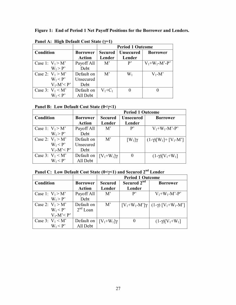
We now consider the various borrower and lender period 1 payoff conditions

assuming extreme values for γ. Figure 1 shows the payoff conditions for the secured and

unsecured lenders as well as the borrower. In Panel A, we assume that γ=1 implying that

the lenders are able to foreclose on the borrower’s assets to satisfy an outstanding claim.

Case 1 shows the payoff positions when the total value of all assets is greater than the

debt outstanding. In this situation, the borrower obviously pays off all loans and has a

7 Pence (2002) confirms this finding using HMDA loan level data. 8 As discussed by Berkowitz and Hynes (1999) and Lin and White (2001), Federal bankruptcy law provides a homestead exemption of $7,500 but each state is allowed to set its own exemption level. As a result, individual state homestead exemption levels vary widely with some being unlimited and others being very restricted. Lin and White (2001) note that personal property exemptions have smaller variation across states.

8

positive wealth position. In Case 2, we show the payoff when the value of the house is

greater than the secured mortgage debt, but period one wealth is less than the unsecured

debt (W1<P’). As a result, the borrower defaults on the unsecured debt and the unsecured

creditor’s recourse is to seize the personal assets to satisfy the unsecured debt P’. Since

the unsecured creditor is unable to attach the borrower’s housing equity, the borrower’s

net period one wealth position is (V1-M’) and the unsecured creditor suffers a net loss

(P’-W1). Finally, Case 3 considers the payoffs if the house value is less than the secured

mortgage amount. This is the classic mortgage default condition triggered by negative

equity. In this situation, the secured lender forecloses on the property and suffers a loss

equal to M’-V1-W1. Nothing remains for the unsecured lender who thus suffers a loss of

P’ and the borrower’s net period one wealth position is zero.

In Panel B, we show the period one payoffs assuming the borrower resides in a

very low default cost state. We assume that the probability of foreclosing and receiving a

payoff in the event of default is positive, but small. Again, Case 1 shows that the payoffs

are the same as in Panel A since the borrower has no financial incentive to default.

However, in Case 2, the payoff to the unsecured lender is smaller since (W1)γ< W1 and

the payoff to the borrower is now (W1(1-γ)+(V1-M’)). Thus, as the cost of default

declines (costs to the lender associated with foreclosure increase), the borrower’s

expectation of keeping a portion of her period one wealth in the event of default

increases. Finally, Case 3 shows that the unsecured lender’s payoff is zero when default

occurs on the secured debt since all assets that can be collected are used to payoff the

secured lender’s position.

9

Panel C shows the period one outcomes assuming that P is now financed with a

secured second mortgage. The payoff conditions in Case 2 are altered to reflect the

ability of the junior secured lender to seize part of the borrower’s housing equity. Since

V1-M’>0, the payoff to the secured second lender is greater than the payoff to the

unsecured lender ([V1+W1-M’]γ> [W1]γ). The secured second lender’s gain is directly

offset by the borrower’s loss; and, as a result, in states where borrower default costs are

low, the unsecured lender has an incentive to entice the borrower to switch from

unsecured debt to secured debt by offering more generous loan terms for junior secured

debt than for unsecured debt.

The implications of our model with respect to borrower quality and loan amount

contrast with the model predictions of Brueckner (1994, 2000), who develops a simple

two-period model of borrower default that examines the impact of borrower risk on

choice of loan amount. Brueckner’s model is based on default being triggered by

declines in the underlying collateral asset value and his analysis implies that low risk

borrowers self-select smaller loans while high-risk borrowers select larger loans. This

result is based on the observation that default costs appear to be important in

understanding the empirical incidence of default. Brueckner’s model follows from the

information asymmetry arguments first applied to the insurance market by Rothschild

and Stiglitz (1976). Rothschild and Stiglitz’s (1976) analysis of the insurance market

demonstrated that when insurers cannot discern risky applicants from non-risky

applicants, the “safe” applicants signal their risk profile by applying for less insurance

than the “risky” applicants. Similarly, Brueckner’s model indicates that, in the presence

10

of non-trivial default costs, only high-risk borrowers are willing to pay the premium for a

high LTV ratio.9

However, our predictions are consistent with those presented by Harrison, et al

(2002), who modify Brueckner’s model to examine the impact of borrower income on

default. Borrower income is not explicitly considered in the original Brueckner model

where default is motivated by changes in house value. Rather than allow default to be

motivated by uncertain future asset values, Harrison, et al (2002) motivate default based

on uncertainty regarding the borrower’s future income (holding the asset value fixed).

Thus, default occurs if the borrower’s future income is insufficient to repay the debt in

the presence of a decline in asset value. With default conditional on income, their model

shows that when default costs are high, risky borrowers choose low LTV ratios to

minimize default costs. However, their model provides additional insights by indicating

that when default costs are low, risky borrowers may actually choose higher LTV ratios.

To summarize, our analysis implies that borrowers in states with low default costs

will have higher secured second loan amounts relative to borrowers in states with high

default costs. Furthermore, our model also implies that secured junior loan amounts

should be directly correlated with borrower credit quality since the lender looks to both

the underlying collateral as well as future income for loan repayment. That is, our model

predicts that higher quality borrowers will have higher loan amounts relative to lower

quality borrowers. This is consistent with the predictions of Harrison et al (2002) and

directly counters to the predictions of Brueckner (1994, 2000). In addition, to the extent

9 Brueckner’s model is consistent with models corporate borrowering. For example, Bolton and Scharfstein (1996) develop a model of debt issuance that predicts that low-risk firms should borrower from a greater number of creditors while high-risk firms will only borrower from a few creditors. Their model also implies that low risk borrowers will have larger second loans relative to high-risk borrowers.

11

that lenders are able to differentiate borrower quality based on credit scores, we expect

that loan costs should be negatively related to borrower credit scores.

IV. Data

In order to test the predictions from our model, we employ a dataset of 132,184

second mortgage loans originated for securitization between 1995 and 1999. This dataset

is unlike most other mortgage datasets in that these mortgages represent second loans that

are secured by the underlying property. However, in many cases, when the original

mortgage loan balance is combined with the second loan amount, the total mortgage debt

exceeds the value of the collateral asset. As a result, these loans are often referred to as

“125% LTV” loans. The “125” designation denotes the fact that the maximum LTV ratio

is normally 125 percent of the property collateral value. In order to make the dataset as

clean as possible, we include only subordinate loans with single-family residential

collateral. The dataset contains information regarding the borrower’s reason for desiring

the mortgage, allowing a test of whether loans originated for the purpose of “debt

consolidation” differ from loans originated for other purposes (home improvement,

refinancing, etc.).

Table 1 shows the distribution of the loans by origination year. We note that the

majority of the mortgages (50%) were originated in 1997. The mortgages were

originated across the US, but have significant concentration in California (21.5%) with

the next highest concentration in Florida (7.8%).10 Consistent with Texas banking laws

10 A table detailing the geographic distribution of mortgages originations is available from the author upon request.

12

regarding second mortgages, there were only 206 loans originated in Texas.

Furthermore, consistent with the findings of Ambrose, LaCour-Little, and Sanders

(2002), we find that the origination spread for high credit quality borrowers is

significantly lower than the origination interest rate spread for low credit quality

borrowers (Table 2).11

In order to estimate the impact of state-specific default laws, we follow the

analysis of Ambrose and Pennington-Cross (2000) who categorize the states based on

whether creditors must use judicial or non-judicial foreclosure and whether the states

have anti-deficiency judgment statutes.12 From the lender’s perspective, this

classification system defines a high default cost state as one that requires judicial

foreclosure proceedings but does not allow deficiency judgments. Similarly, a low

default cost state is one that does not require judicial foreclosure and allows lenders to

obtain deficiency judgments against borrower assets.

Given that deficiency judgments increase the risk to the borrower, the theory

proposed by Harrison et al (2002) suggests that borrowers in states that allow deficiency

judgments should self select lower debt amounts than borrowers in states that limit

deficiency judgments, all else being equal. As a preliminary test of this hypothesis, we

report in Table 3 the mean total debt loan-to-value ratio and senior debt loan-to-value

ratios based on whether or not the borrower lives in a state that allows deficiency

judgments. We find that borrowers in states that have do not allow deficiency judgments

11 The origination interest rate spread is defined as the mortgage contract rate at origination less the 10-year Treasury rate at date of origination. 12 Judicial foreclosure proceeding are more costly and time-consuming than non-judicial proceedings since creditors are required to obtain a court order to foreclosure on the property to satisfy the debt. Anti-deficiency judgment statutes prohibit creditors from attaching other assets or garnishing future wages to satisfy losses that occur due to default.

13

carry significantly higher senior debt amounts but lower total debt amounts than

borrowers in states that allow deficiency judgments.

Since judicial foreclosure has the perception of providing greater borrower

protection than non-judicial foreclosure proceedings, total debt amounts and junior loan

amounts in states that require judicial foreclosure should be higher than in states that

allow non-judicial foreclosure. Thus, Table 3 also reports the mean total loan-to-value

ratios and senior loan-to-value ratio classified by state law regarding foreclosure.

Contrary to expectations, we find that mean senior loan-to-value ratios are significantly

lower in states that require judicial foreclosure.13 However, total debt loan-to-value ratios

are higher in states that require judicial foreclosure. Since default costs are in general a

zero sum game (borrower protections limit lender default recovery and pro lender

regulations increase potential borrower losses), one possible explanation for this result is

that lenders may ration credit in states where legal regulations limit lender abilities to

quickly recover assets in case of default. Since most borrowers in default do not have

other assets to attach, lenders may view deficiency judgments as less important than the

ability to utilize non-judicial foreclosure proceedings.

When factoring borrower credit and information signaling, Harrison et al (2002)

suggest that holding default costs constant, high quality borrowers in high default cost

states self-select higher loan amounts while low quality borrowers self select lower loan

amounts to minimize the potential cost of default. Therefore, we test whether higher risk

borrowers select larger loans and whether higher risk borrowers in high default cost states

select lower loan amounts, holding all else constant. Table 4 shows the differences in

mean loan-to-value ratios based on whether the borrower’s FICO score is greater than or 13 This is consistent with the findings of Pence (2002).

14

less than the average FICO score in the sample. Consistent with our theory, higher

quality borrowers do have significantly higher senior loan amounts. However, lower

quality borrowers have higher loan-to-values based on total debt. This finding is

inconsistent with the debt-signaling hypothesis proposed by Bolton and Scharfstein

(1996). Holding all else constant, Bolton and Scharfstein’s (1996) theory is that lower

risk borrowers will have larger second loans as they are in a position to take on more

debt.

In the regression analysis discussed below, we test whether lenders price loans

based on borrower risk and default costs. Merton (1974) predicts that borrower yield

spreads are a positive function of total debt. In contrast, the model predicts that lenders

will offer borrowers lower spreads to entice them to switch from unsecured personal debt

to secured mortgage debt. This last test should provide insight into the question of

whether lenders engage in predatory lending practices by charging interest rates unrelated

to borrower credit risk.

V. Empirical Modeling

One of the primary problems with analyzing the impact of state level default costs

on the availability of credit is the endogenous relationship between the mortgage loan

terms, the loan amount, the collateral quality, and the borrower’s credit quality. This

endogenous relationship is widely recognized in the literature that examines borrower

choice concerning loan amount and housing consumption. For example, Ambrose,

LaCour-Little, and Sanders (2002) employ a simultaneous equations system to recognize

15

the well-known endogenous relationship between LTV and house value.14 However, our

analysis is more complicated in that we examine the borrower’s choice of junior loan

debt and the impact of default costs on the availability and cost of that debt. In this

context, the amount of housing consumption is already determined. Thus, the

endogenous terms are related to the amount of the second loan, its costs (interest rate

spread), and loan term, assuming that the borrower’s house (collateral) value, credit

quality and income are exogenous to the decision. Therefore, to control for this

endogenous relationship we estimate the following system via non-linear three-stage least

squares regression (3SLS):

( )

ik

ikj

ij

r

iiiii

treasmktiiii

QtrDUMYrDUM

adcreditspreyieldcurveimprovecashoutdebtconsolDJ

rrFICOTermloanamtSpread

treas

εαα

αασαααααα

ααααα

+++

++++++++

−++++=

∑∑==

19

17

16

13

121110

98765

43210 )log(

(1.)

( )

ik

ikj

ij

iiii

iiii

QtrDUMYrDUMimprovecashout

debtconsolDJFICOhouselfirstmtgbaTermSpreadloanamt

εββββ

βββββββββ

+++++

++++++++=

∑∑==

17

15

14

11109

87654

3210log (2.)

ik

ikj

iji

iiiii

QtrDUMYrDUMD

JFICOloanamtSpreadTerm

εγγγ

γγγγγ

++++

++++=

∑∑==

12

10

9

65

43210 )log( (3.)

14See Ling and McGill (1998) for an example of a simultaneous equation model where mortgage demand is a function of borrower income, nonhousing wealth, desired housing consumption, and demographic characteristics, and housing consumption is a function of the level of mortgage debt as well as economic and demographic factors.

16

where Spreadi is the second mortgage origination spread, loanamti is the second (junior-

secured) loan amount, Termi is the term of the second loan, rmkt is the current mortgage

rate as proxied by the Freddie Mac 30-year fixed-rate mortgage rate, rtreas is the 10-year

constant maturity treasury rate, yieldcurve is the market yield curve (10-year constant

maturity treasury rate less the 1-year constant maturity treasury rate), creditspread is the

bond market credit risk spread as proxied by the difference in the BAA and AAA

corporate bond rates, FICOi is borrower i’s credit score at origination, housei is the value

of the house at second loan origination, firstmtgamti is the first (senior) mortgage amount,

debtconsoli is the percent of the second loan used for debt consolidation purposes,

cashouti is the percent of the second loan that is taken as cash at closing, improvei is the

percent of the second loan used for home improvement purposes, D is a dummy variable

denoting states that allow lenders to pursue deficiency judgments against borrowers in

default, J is a dummy variable denoting states that require judicial foreclosure

proceedings, YrDUM is a series of dummy variables denoting the year of origination

(1996-1999 with 1995 being the reference year), and QtrDUM is a series of three dummy

variables denoting the origination quarter (the first quarter is the reference).

The origination Spread is calculated as the effective yield assuming a 10-year

holding period less the 10-year constant maturity treasury rate. In calculating the

effective yield, we include the impact of closing costs and points. Approximately 10% of

the sample had missing or incorrectly coded closing cost amounts. Thus, we imputed the

closing costs on loans with missing data using the mean closing cost amount for the top

75 percent of the sample. The dataset does not contain actual information about the

points charged to borrowers; however, discussions with lender representatives indicate

17

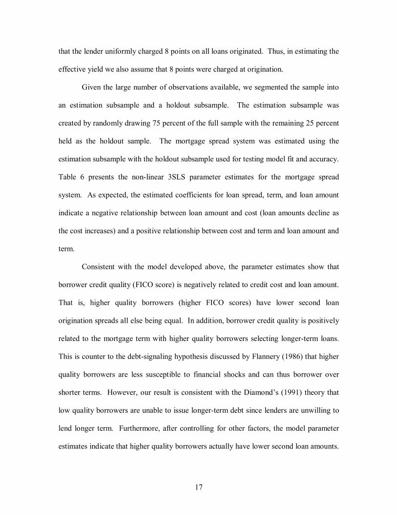
that the lender uniformly charged 8 points on all loans originated. Thus, in estimating the

effective yield we also assume that 8 points were charged at origination.

Given the large number of observations available, we segmented the sample into

an estimation subsample and a holdout subsample. The estimation subsample was

created by randomly drawing 75 percent of the full sample with the remaining 25 percent

held as the holdout sample. The mortgage spread system was estimated using the

estimation subsample with the holdout subsample used for testing model fit and accuracy.

Table 6 presents the non-linear 3SLS parameter estimates for the mortgage spread

system. As expected, the estimated coefficients for loan spread, term, and loan amount

indicate a negative relationship between loan amount and cost (loan amounts decline as

the cost increases) and a positive relationship between cost and term and loan amount and

term.

Consistent with the model developed above, the parameter estimates show that

borrower credit quality (FICO score) is negatively related to credit cost and loan amount.

That is, higher quality borrowers (higher FICO scores) have lower second loan

origination spreads all else being equal. In addition, borrower credit quality is positively

related to the mortgage term with higher quality borrowers selecting longer-term loans.

This is counter to the debt-signaling hypothesis discussed by Flannery (1986) that higher

quality borrowers are less susceptible to financial shocks and can thus borrower over

shorter terms. However, our result is consistent with the Diamond’s (1991) theory that

low quality borrowers are unable to issue longer-term debt since lenders are unwilling to

lend longer term. Furthermore, after controlling for other factors, the model parameter

estimates indicate that higher quality borrowers actually have lower second loan amounts.

18

This is counter to the simple comparison of means reported earlier. However, this result

is consistent with Brueckner’s (2000) theory that, in equilibrium, higher quality

borrowers do not request larger loan amounts.

The model coefficients provide strong support for a positive relationship between

borrowers in states that require judicial foreclosure proceedings and the second loan

terms. The parameter estimates indicate that borrowers in states that require judicial

foreclosure have higher second loan amounts, pay more for the loan (origination spread is

larger), and borrower over a shorter term. However, we find the opposite effect for states

that limit borrower deficiency judgments. The negative coefficients for deficiency

judgments in the spread and loan amount equations indicate that borrowers in states that

prevent lenders from seeking deficiency judgments have lower spreads and loan amounts.

This is consistent with the theory that lenders tradeoff loan costs with loan amounts. The

results are also consistent with the theory that lenders restrict credit in states with

regulations that limit their ability to recover losses (anti-deficiency judgment statutes)

whereas lenders do not restrict credit in states that simply increase the costs associated

with default (require judicial foreclosure) but do not limit the lender’s ability to recover

losses.

The coefficients regarding the use of funds do not reveal a significant relationship

between loan amount or cost and the percentage of funds used to consolidate other debts.

However, we do find that that the cost of second loan debt is significantly lower as the

percentage of the loan amount used for home improvements or cash out increases. At the

same time, borrowers seeking loans for home improvements or to cash out also have

lower amounts.

19

Examining the other macro economic and borrower specific factors, we see that

borrowers with higher house values have higher second loan amounts while borrowers

with larger first mortgages have lower second mortgages. We also find that the cost of

second loans is positively related to the mortgage market interest rate spread and the

overall market credit risk premium (corporate bond credit risk spread). This is consistent

with a number of previous studies who find that the mortgage market is integrated with

the larger capital markets.15

VI. Model Predictions

In Table 7 we report the mean and median spread, second loan amount, and loan

term prediction errors for the estimation sample using the parameter estimates reported in

Table 6. Since the mean prediction errors can be skewed by extreme outliers, we chose

to focus on the median values. The first row reports the mean and median prediction

errors (residuals) for the full sample. The median values indicate that the model tends to

underfit the spread and overfit the loan amount and term. We next divide the sample

based on borrower FICO score and note that the spread prediction error appears to be

smaller for the low FICO sample (FICO scores less than 684). For the high FICO

subsample, the predicted spread is 25 basis points lower than the actual while the median

error for the low FICO subsample is only 0.76 basis points lower. We also estimate the

impact of the borrower’s reason for the originating the second loan. Analysis of the

residuals indicates that the prediction error is highest for borrowers using at least 90% of

the loan amount for debt consolidation (123 basis points for high FICO borrowers and 94

basis points for low FICO borrowers).

15 For example, see Gonzalez-Rivera (2001) and Kolari, Fraser, and Anari (1998) for example.

20

We also examine the prediction errors for high quality and low quality borrowers

based on their state default regulations. We classify high default cost states (from the

lender’s perspective) as states that require judicial foreclosure proceedings (J=1) but do

not allow deficiency judgments (D=1). Low default cost states are classified as those that

do not require judicial foreclosure (J=0) but allow deficiency judgments (D=0).

Interestingly, we find that the spread prediction error is uniformly negative (model over

predicts the spread) across all state default regulation categories for the high quality

borrower subsample. However, the model appears to uniformly under predict loan costs

for the low FICO subsample (errors are positive). In the final section of Table 7, we

highlight the prediction errors for high and low default cost states based on borrower

quality assuming funds used for debt consolidation. The model errors are slightly greater

for states with high default costs.

In Table 8 we assess the estimated systems predicted accuracy using the hold-out

sample as an out-of-sample test. Predicted spread, loan amount, and term were estimated

via Newton’s method for each observation in the holdout sample using the parameter

coefficients reported in Table 6. Since this is an “out-of-sample” test, the mean

prediction errors for the full sample are no longer zero. The results indicate that the

system has a relatively high predictive accuracy. The mean spread error is 0.1 basis

points and the median spread error is 12 basis points. As in Table 7, we find that the

model tends to over estimate the spread for high quality borrowers and under predict the

spread for low quality borrowers. However, the degree of error is larger for high quality

borrowers than for low quality borrowers.

21

By controlling for borrower risk characteristics, interrelated loan terms, market

conditions, and state-level default laws, we are able assess the degree of under- or over-

pricing of junior secured mortgages. We create a series of hypothetical borrowers

differentiated by risk and location. For example, we segment the holdout sample into

very high and very low quality borrowers where very high quality is defined as any

borrower with a FICO score above the 75th percentile of the whole sample (FICO>706)

and very low quality is defined as any borrower with a FICO score below the 25th

percentile of the whole sample (FICO < 658). Next we calculate the independent

variable means for these high and low quality subsamples further segmented by whether

their state requires judicial foreclosure (J=1) or does not allow deficiency judgments

(D=1). Using the relevant mean values of these hypothetical borrowers, we then estimate

predicted loan spreads, term, and amounts. Comparing these predicted values to the

actual means for each borrower segment will allow us to quantify the degree of lender

under or over pricing.

Table 9 shows the comparison for borrowers living in high default cost and low

default cost states. Consistent with the prediction errors reported above, we see that

predicted as well as actual spreads are lower in low default cost states. However, it is

interesting to note that low quality borrowers are consistently over-charged relative to the

model predictions. For example, the interest rate charged on a loan to a low quality

borrower living in a high cost state was, on average, 64 basis points higher than the

predicted value. On the other hand, high quality borrowers living in states with high

default costs were consistently under charged by 18 basis points, on average.

22

VII. Summary and Conclusions

The high LTV mortgage examined in this paper is an interesting twist on the

home equity loan contract in that it has a higher interest rate and aggregate LTV than

traditional home equity loans. As the market continues to grow for the various

permutations of home equity loans, the impact of credit on mortgage rates becomes quite

important (particularly when compared to conforming first mortgages purchased by the

government sponsored agencies where credit risk is of little concern).

In this paper, we examine the pricing of high-LTV debt and determine whether

state-specific default laws have an impact on the availability and cost of that debt. First,

we find that lenders rationally price loans to higher risk borrowers for the most part;

however, when we focus on smaller and smaller FICO scores buckets, the results indicate

that the mean actual loan rates are higher than those predicted by our model. Second, we

examine the impact of borrower protection laws on the price of credit and if borrowers in

states that limit the lender’s ability to seek default remedies pay higher credit costs; we

find that states that do not require judicial foreclosure and allow deficiency judgments on

high LTV loans have lower lending rates (by about 33 basis points) than loans in states

that require judicial foreclosure and do not allow deficiency judgments. Third, we find

that there is a greater degree of error in the pricing of high LTV loans to low FICO

borrowers than to high FICO borrowers. Stated in a different way, it is more difficult to

explain the rate charged to lower credit risk borrowers in that the rates charged are higher

than those predicted by our “rational” model of loan pricing.

23

REFERENCES

Ambrose, B.W., and R.J. Buttimer, Jr. “Embedded Options in the Mortgage Contract.” The Journal of Real Estate Finance and Economics 21:2 (2000), 95-111. Ambrose, B.W., R.J. Buttimer, Jr., and C.A. Capone, Jr. “Pricing Mortgage Default and Foreclosure Delay.” Journal of Money, Credit, and Banking 29:3 (1997), 314-325. Ambrose, B.W., and A. Pennington-Cross. “Local Economic Risk Factors and the Primary and Secondary Mortgage Markets.” Regional Science and Urban Economics 30:6 (2000), 683-701. Ambrose, B.W., M. Lacour-Little, and A. Sanders. “Credit Spreads and Capital Structure: Evidence from the Mortgage Market”, Ohio State University Working Paper (2002).

Berkowitz, J. and R. Hynes. “Bankruptcy Exemptions and the Market for Mortgage Loans.” Journal of Law and Economics 42 (1999), 809-830. Bolton, P. and D. Scharfstein. “Optimal debt structure and the number of creditors.” Journal of Political Economy 104:1 (1996), 1-25. Brueckner, J.K. “Mortgage Default with Asymmetric Information.” Journal of Real Estate Finance and Economics 20 (2000), 251-275. Brueckner, J.K. “Unobservable Default Propensities, Optimal Leverage, and Empirical Default Models: Comments on ‘Bias in Estimates of Discrimination and Default in Mortgage Lending: The Effects of Simultaneity and Self-Selection’.” Journal of Real Estate Finance and Economics 9:3 (1994), 217-222. Diamond, D. “Debt Maturity Structure and Liquidity Risk.” Quarterly Journal of Economics (1991), 709-737. Flannery, M. “Asymmetric Information and Risky Debt Maturity Choice.” Journal of Finance 41 (1986), 18-38. Gonzalez-Rivera, G. “Linkages Between Secondary and Primary Markets for Mortgages.” Journal of Fixed Income (2001), 29-36. Harrison, D.M., T.G. Noordewier, and A. Yavas. “Do Riskier Borrowers Borrow More?”. Pennsylvania State University Working Paper (2002). Kau, J.B. and D.C. Keenan. “An Overview of the Option-Theoretic Pricing of Mortgages.” Journal of Housing Research 6:2 (1995), 217-244.

24

Kolari, J.W., D.R. Fraser, and A. Anari. “The Effects of Securitization on Mortgage market Yields: A Cointegration Analysis.” Real Estate Economics 26:4 (1998), 677-693 Lin, E.Y., and M.J. White. “Bankruptcy and the Market for Mortgage and Home Improvement Loans.” Journal of Urban Economcis 50 (2001), 138-162. Ling, D.C., and G.A. McGill. “Evidence on the Demand for Mortgage Debt by Owner-Occupants.” Journal of Urban Economics 44 (1998), 391-414. Merton, R.C. “Theory of Rational Option Pricing.” Bell Journal of Economics 4 (1974), 141-183. Pence, K.M. “Foreclosing on Opportunity: State Laws and Mortgage Credit.” Board of Governors of the Federal Reserve System working paper (2002). Quercia, R., and M.A. Stegman. “Residential Mortgage Default: A Review of the Literature.” Journal of Housing 3 (1992), 341-380. Rothschild, M. and J. Stiglitz. “Equilibrium in Competitive Insurance Markets: An Essay on the Economics of Imperfect Information.” Quarterly Journal of Economics 90 (1976), 629-649.

25

Chart 1. Historical Prepayments for Three Mortgage Products.

Historical Prepayment

0.00%

10.00%

20.00%

30.00%

40.00%

50.00%

60.00%

70.00%

Dec

-97

Feb-

98

Apr

-98

Jun-

98

Aug

-98

Oct

-98

Dec

-98

Feb-

99

Apr

-99

Jun-

99

Aug

-99

Oct

-99

Dec

-99

Feb-

00

Apr

-00

Jun-

00

Aug

-00

Age of Collateral (months)

CPR

FIRSTPLUS 125 LTV97-1 Money Store Home Equity 1996-D RFMSI Whole Loan

26

Chart 2. Historical 90-day Delinquency for Three Mortgage Products.

Historical 90 Day Delinquency

0.00%2.00%4.00%6.00%8.00%

10.00%12.00%14.00%16.00%18.00%

Dec

-97

Feb-

98

Apr

-98

Jun-

98

Aug

-98

Oct

-98

Dec

-98

Feb-

99

Apr

-99

Jun-

99

Aug

-99

Oct

-99

Dec

-99

Feb-

00

Apr

-00

Jun-

00

Age of Collateral (months)

90 D

ay D

elin

quen

cy

FIRSTPLUS 125 LTV97-1 Money Store Home Equity 1996-D RFMSI Whole Loan

Source: Bloomberg.

27

Figure 1: End of Period 1 Net Payoff Positions for the Borrower and Lenders. Panel A: High Default Cost State (γ=1) Period 1 Outcome Condition Borrower

Action SecuredLender

UnsecuredLender

Borrower

Case 1: V1 > M’ W1 > P’

Payoff All Debt

M’ P’ V1+W1-M’-P’

Case 2: V1 > M’ W1 < P’ V1-M’< P’

Default on Unsecured

Debt

M’ W1 V1-M’

Case 3: V1 < M’ W1 < P’

Default on All Debt

V1+C1 0 0

Panel B: Low Default Cost State (0<γ<1) Period 1 Outcome Condition Borrower

Action Secured Lender

UnsecuredLender

Borrower

Case 1: V1 > M’ W1 > P’

Payoff All Debt

M’ P’ V1+W1-M’-P’

Case 2: V1 > M’ W1 < P’ V1-M’< P’

Default on Unsecured

Debt

M’ [W1]γ (1-γ)[W1]+ [V1-M’]

Case 3: V1 < M’ W1 < P’

Default on All Debt

[V1+W1]γ 0 (1-γ)[V1+W1]

Panel C: Low Default Cost State (0<γ<1) and Secured 2nd Lender Period 1 Outcome Condition Borrower

Action Secured Lender

Secured 2nd Lender

Borrower

Case 1: V1 > M’ W1 > P’

Payoff All Debt

M’ P’ V1+W1-M’-P’

Case 2: V1 > M’ W1 < P’ V1-M’< P’

Default on 2nd Loan

M’ [V1+W1-M’]γ (1-γ) [V1+W1-M’]

Case 3: V1 < M’ W1 < P’

Default on All Debt

[V1+W1]γ 0 (1-γ)[V1+W1]

28

Table 1: Distribution by Origination Year Year Frequency Percent 1995 495 0.4 1996 14,212 10.8 1997 65,977 49.9 1998 50,929 38.5 1999 571 0.4 Total 132,184 100.0

Table 2: Mean Loan Origination Spread by Borrower FICO Score (Standard Deviations in parentheses) Borrower Fico Range mean std dev [0, 658) 15.38 2.29[658, 682) 14.09 2.06[682, 706) 13.07 1.88[706+) 12.50 1.89 Table 3: Mean Loan Amounts Classified by State Foreclosure Laws. (Standard Deviations in parentheses)

Deficiency Judgments Judicial Foreclosure

Allowed Not

Allowed t-stat. Required Not

required t-stat. Senior Debt LTV 79.28 82.71 43.7*** 77.78 81.84 46.1***

(14.54) (13.60) (15.03) (13.88) Total Debt LTV 111.28 109.84 -19.9*** 111.48 110.39 -14.1***

(12.45) (13.01) (12.65) (12.70) N 79,831 52,353 93,167 39,017

Note: t-statistic test for equality of means under assumption of unequal variance. ***significant at the 1% level.

29

Table 4: Mean Loan Amounts Classified by Borrower FICO Score. (Standard Deviations in parentheses)

FICO Scores

High FICO

Low FICO t-stat.

Senior Debt LTV 79.63 51.82 24.0***

(14.53) (13.99) Total Debt LTV 110.08 111.26 16.8***

(13.10) (12.31) N 61,473 70,711

Note: t-statistic test for equality of means under assumption of unequal variance. High FICO borrowers have FICO scores greater than the mean FICO score for the sample (684) and Low FICO borrowers have FICO scores less than or equal to the mean FICO score for the sample.

***significant at the 1% level.

30

Table 5: Descriptive Statistics Variable Label N Mean Std Dev Original_Interest_Rate Junior Mortgage Interest Rate 132184 13.60 1.50Loanamt Junior Mortgage Loan Amount 132184 $31,699.92 $12,095.56Yield Junior Mortgage Effective Interest Rate 132184 19.629 2.302Spread Junior Mortgage Origination Spread 132184 13.746 2.307 Firstmtgbal First Mortgage Loan Amount 132184 $94,231.82 $45,891.29Value House Value (Appraised) 132184 $114,695.56 $49,883.17Loan_To_Value Loan_To_Value (total debt) 132184 110.709 12.693FICO Borrower FICO Score 132184 683.314 35.590 rmkt 30 - Fixed Conventional Market Rate 132184 7.396 0.417Yieldcurve 10 year Treasury - 1 year Treasury 132184 0.514 0.317

treasrσ Standard Deviation of 10-year Treasury 132184 0.305 0.085Creditspread Baa - AAA Bond Spread 132184 0.627 0.065 J 1=require judicial 132184 0.295 0.456D 1=allows deficiency 132184 0.604 0.489

31

Table 6: Non-linear Three-Stage Least Squares Estimation of Mortgage Origination Terms

(t-statistics reported in parentheses) Spread log(loanamt) Term

Intercept 61.496*** 7.553*** -325.231***

(81.25) (26.28) -(23.81) Spread -0.098*** 4.211***

-(14.39) (13.64) log(loanamt) -6.139*** 43.803***

-(38.83) (121.03) Term 0.118*** 0.022***

(31.41) (111.41) FICO -0.014*** -4.30E-04* 0.016*

-(20.58) -(1.84) (1.60) debtconsol 4.40E-04 0.001

(0.02) (0.44) homeimprove -0.920*** -0.011***

-(15.23) -(2.96) cashout -1.048*** -0.013***

-(15.65) -(3.31) J 0.278*** 0.045*** -1.951***

(7.29) (4.29) -(4.16) D -1.266*** -0.227*** 10.036***

-(26.27) -(22.53) (22.34) (rmkt-rtreas) 0.349***

(7.37)

treasσ -0.576*** -(3.95)

yieldcurve 0.751*** (5.53)

creditspread 3.584*** (13.73)

firstmtgbal -5.61E-08* -(1.62)

Value 1.07E-07*** (4.36)

Yr96 -2.841*** -0.363*** 16.074***

-(9.96) -(5.09) (4.99) Yr97 -4.899*** -0.807*** 35.723***

-(16.29) -(11.37) (11.20) Yr98 -8.063*** -1.513*** 67.279***

-(23.35) -(20.94) (21.10) Yr99 -7.106*** -1.169*** 52.136***

-(14.00) -(9.56) (9.56) Qtr2 0.095 0.165** -7.551***

(0.35) (2.23) -(2.26) Qtr3 -0.519* 0.010 -0.595

-(1.93) (0.14) -(0.18) Qtr4 -1.478*** -0.220*** 9.712***

-(5.49) -(3.01) (2.94)

32

***significant at the 1% level. **significant at the 5% level. *significant at the 10% level.

33

Table 7: Mean (Median) Prediction Errors (Estimation Sample) (Actual – Predicted)

Number of

Observations Spread Log(Amount) Term Full Sample 99,128 0.0000 0.0000 0.0000 -(0.1266) (0.0264) (21.4125) High Fico Borrower 47,155 -0.1335 0.0016 -0.3102 -(0.2500) (0.0303) (21.6336)Low FICO Borrower 51,973 0.1211 -0.0015 0.2815 -(0.0076) (0.0233) (21.2488)High FICO Borrower Debt Consolidation 4,891 -1.1518 -0.1316 -20.6670 -(1.2313) -(0.0929) -(4.0076) Home Improvement 984 -0.0740 0.0723 6.0451 -(0.4612) (0.1725) (12.8743) Cash Out 1,134 -0.2369 0.2444 5.2756 -(0.3230) (0.2867) (10.3322)Low FICO Borrower Debt Consolidation 6,508 -0.9254 -0.0998 -11.4102 -(0.9373) -(0.0534) (8.2084) Home Improvement 1,569 -0.1870 0.1901 8.1556 -(0.5444) (0.2878) (15.9529) Cash Out 132 -0.7798 0.1540 -3.8320 -(0.7495) (0.1385) (4.5451)High FICO Borrower Judicial=0, Deficiency = 0 14,983 -0.1815 0.0162 1.0175 -(0.2951) (0.0334) (26.3948) Judicial=0, Deficiency = 1 18,864 -0.0667 -0.0178 -1.9679 -(0.2221) (0.0301) (14.7209) Judicial=1, Deficiency = 0 12,287 -0.1835 0.0016 0.3964 -(0.2550) (0.0165) (27.8560) Judicial=1, Deficiency = 1 1,021 -0.0615 0.1462 2.3289 -(0.0334) (0.1395) (30.5895)Low FICO Borrower Judicial=0, Deficiency = 0 17,839 0.1803 0.0000 -0.4268 (0.0291) (0.0205) (23.1725) Judicial=0, Deficiency = 1 18,183 0.0419 0.0052 1.6218 -(0.0874) (0.0460) (17.0591) Judicial=1, Deficiency = 0 14,859 0.1183 -0.0177 -0.8415 (0.0180) -(0.0043) (24.5719) Judicial=1, Deficiency = 1 1,092 0.5123 0.0852 4.8119 (0.3769) (0.0950) (27.3471)High FICO Borrower, Debt Consolidation Low Cost (J=0, D=0) 1,751 -1.1267 -0.1076 -17.9652 -(1.1466) -(0.0851) -(3.0290) High Cost (J=1, D=1) 69 -1.3798 -0.0603 -32.0205 -(1.1720) -(0.0260) -(30.2281)Low FICO Borrower, Debt Consolidation

34

Low Cost (J=0, D=0) 2,494 -0.8270 -0.0854 -12.3726 -(0.8542) -(0.0410) (6.3782) High Cost (J=1, D=1) 83 -0.8566 -0.0459 -13.8616 -(0.9305) -(0.0601) (14.4214) Note: High FICO borrower sample include all borrowers with FICO scores greater than or equal to 684 and the low FICO borrower sample include all borrowers with FICO scores less than or equal to 683. Fund utilization samples are all borrowers utilizing greater than 90% of funds for the purpose identified.

35

Table 8: Mean (Median) Prediction Errors (Random Holdout Sample). Predictions obtained from coefficients estimated on 75% random sample. High FICO Borrower sample have FICO scores greater than or equal to 684 and the low FICO Borrower sample have FICO scores less than or equal to 683. (Actual – Predicted)

Number of

Observations Spread Log(Amount) Term Full Sample 33,056 -0.0010 0.0051 0.3406 -(0.1203) (0.0269) (20.9147) High Fico Borrower 15,867 -0.1355 0.0064 -0.0897 -(0.2497) (0.0328) (21.8026)Low FICO Borrower 17,189 0.1233 0.0039 0.7378 (0.0069) (0.0229) (20.1700)High FICO Borrower Debt Consolidation 1,656 -1.1091 -0.1429 -18.8407 -(1.2117) -(0.0934) (2.7961) Home Improvement 311 0.0413 0.0787 6.5076 -(0.3991) (0.2049) (19.3227) Cash Out 335 -0.3111 0.1954 7.0499 -(0.4818) (0.2805) (7.9445)Low FICO Borrower Debt Consolidation 2,163 -0.9747 -0.1013 -10.1066 -(0.9709) -(0.0522) (9.9774) Home Improvement 481 -0.1593 0.3707 19.2671 -(0.7301) (0.2568) (16.0577) Cash Out 39 -0.9877 0.2099 6.2720 -(1.0412) (0.2963) -(8.7189)High FICO Borrower Judicial=0, Deficiency = 0 5,020 -0.1481 0.0267 -0.1111 -(0.2807) (0.0397) (25.8882) Judicial=0, Deficiency = 1 6,341 -0.1018 -0.0179 -0.8099 -(0.2471) (0.0238) (16.0214) Judicial=1, Deficiency = 0 4,187 -0.1648 0.0080 0.9720 -(0.2283) (0.0264) (28.7814) Judicial=1, Deficiency = 1 319 -0.2254 0.1484 0.6268 -(0.1959) (0.1575) (26.2334)Low FICO Borrower Judicial=0, Deficiency = 0 5,775 0.1557 0.0011 1.3329 (0.0715) (0.0275) (23.3103) Judicial=0, Deficiency = 1 6,162 0.0482 0.0178 1.5119 -(0.1189) (0.0354) (15.4308) Judicial=1, Deficiency = 0 4,881 0.1608 -0.0193 -0.6048 (0.0462) -(0.0065) (24.1994) Judicial=1, Deficiency = 1 371 0.3733 0.1216 -3.7221 (0.4573) (0.1147) (24.0928)High FICO Borrower, Debt Consolidation Low Cost (J=0, D=0) 574 -1.2218 -0.1009 -18.8487

36

-(1.2058) -(0.0567) (4.7627) High Cost (J=1, D=1) 28 -1.4715 0.0495 -34.7247 -(1.6136) (0.0716) -(11.0780)Low FICO Borrower, Debt Consolidation Low Cost (J=0, D=0) 766 -0.8823 -0.0948 -10.1004 -(0.9507) -(0.0507) (9.0993) High Cost (J=1, D=1) 38 -1.4532 0.1127 -13.1733 -(1.0207) (0.1019) -(20.1656) Note: Estimation sample created by drawing a 75% random sample of the full sample with the remaining 25% used to test the model fit. High FICO borrower sample includes all borrowers with FICO scores greater than or equal to 684 and low FICO borrower sample includes all borrowers with FICO scores less than or equal to 683. Fund utilization samples are all borrowers utilizing greater than 90% of funds for the purpose identified.

37

Table 9: Actual versus Predicted Loan Terms Mean Values Predicted Values Spread Log(Amount) Term Spread Log(Amount) Term High FICO Borrower Low Cost (J=0, D=0) 12.67 10.32 240.81 12.59 10.30 240.62 High Cost (J=1, D=1) 12.75 10.36 242.65 12.93 10.20 250.12 Low FICO Borrower Low Cost (J=0, D=0) 15.53 10.18 239.51 15.06 10.20 237.78 High Cost (J=1, D=1) 15.86 10.21 250.30 15.22 10.15 251.69

High FICO Borrower subsample includes all borrowers with FICO scores in the 75th percentile. Low FICO Borrower subsample includes all borrowers with FICO scores in the 25th percentile. Predicted values are estimated using mean values of the independent variables in each respective subsample.