Embed Size (px)
Citation preview
Hierarchical Sampling from Sketches: Estimating Functions over
Data Streams
Sumit Ganguly1 and Lakshminath Bhuvanagiri2
1 Indian Institute of Technology, Kanpur2 Google Inc., Bangalore
Abstract. We present a randomized procedure named Hierarchical Sampling from Sketches
(HSS) that can be used for estimating a class of functions over the frequency vectorf of up-
date streams of the formΨ(S) =∑n
i=1 ψ(|fi|). We illustrate this by applying the HSStechnique
to design nearly space-optimal algorithms for estimating thepth moment of the frequency vector,
for realp ≥ 2 and for estimating the entropy of a data stream.3
1 Introduction
A variety of applications in diverse areas, such as, networking, database systems, sensor net-
works, web-applications, share some common characteristics, namely, that data is generated
rapidly and continuously, and must be analyzed in real-time and in a single-pass over the data
to identify large trends, anomalies, user-defined exception conditions, etc.. Furthermore, it is
frequently sufficient to continuously track the “big picture”, or, an aggregate view of the data.
In this context, efficient and approximate computation with bounded error probability is of-
ten acceptable. The data stream model presents a computational model for such applications,
where, incoming data is processed in an online fashion using sub-linear space.
1.1 The data stream model
A data streamS is viewed as a sequence of records of the form(pos, i, v), where,posis the
index of the record in the sequence,i is the identity of an item in[1, n] = 1, . . . , n, and
v is thechangeto the frequency of the item.v > 0 indicates an insertion of multiplicity
v, while v < 0 indicates a corresponding deletion. The frequency of an itemi, denoted by
fi, is the sum of the changes to the frequency ofi since the inception of the stream, that
3 Preliminary version of this paper appeared as the following conference publications. “Simpler algorithm for es-
timating frequency moments of data streams”, Lakshminath Bhuvanagiri, Sumit Ganguly, Deepanjan Kesh and
Chandan Saha,Proceedings of the ACM Symposium on Discrete Algorithms, 2006, pp. 708-713 and “Estimat-
ing Entropy over Data Streams”, Lakshminath Bhuvanagiri and Sumit Ganguly,Proceedings of the European
Symposium on Algorithms, Springer LNCS Volume 4168, pp. 148-159, 2006.

is, fi =∑
(pos,i,v) appears inS v. The following variations of the data stream model have been
considered in the research literature.
1. The insert-onlymodel, where, data streams to not have deletions, that is,v > 0 for all
records. Theunit insert-onlymodel is a special case of the insert-only model, where,
v = 1 for all records.
2. Thestrict update model, where, insertions and deletions are allowed, subject to the con-
straint thatfi ≥ 0, for all i ∈ [1, n].3. Thegeneral update modelwhere no constraints are placed on insertions and deletions.
4. The sliding window model, where, a window size parameterW is given and only the
portion of the stream that has arrived within the lastW time units is considered to be
relevant. Records that are not part of the the current window are deemed to have expired.
In the data stream model, an algorithm must perform its computations in an online manner,
that is, the algorithm gets to view each stream record exactly once. Further, the computa-
tion is constrained to use sub-linear space, that is,o(n logF1) bits, where,F1 =∑n
i=1|fi|.This implies that the stream cannot be stored in its entirety and summary structures must be
devised to solve the problem.
We say that an algorithm estimates a quantityC with ε-accuracy and probability1 − δ
if it returns an estimate that satisfies|C − C| ≤ εC with probability1 − δ. The probability
is assumed to hold for every instance of input data and is taken over the random coin tosses
used by the algorithm. More simply, we say that a randomized algorithm estimatesC with
ε-accuracy if it returns an estimate satisfying|C − C| ≤ εC with constant probability greater
than 12 (for e.g., 7
8 ). Such an estimator can be used to obtain another estimator forC that
is ε-accurate and is correct with probability1 − δ by following the standard procedure of
returning the the median ofs = O(log 1δ ) independent such estimatesC1, . . . , Cs.
In this paper, we consider two basic problems in the data streaming model, namely, esti-
mating the moment of the frequency vector of a data stream and estimating the entropy of a
data stream. We first define the problems and review the research literature.
1.2 Previous work on estimatingFp for p ≥ 2
For any realp ≥ 0, thepth moment of the frequency vector of the streamS is defined as
Fp(S) =n∑
i=1
|fi|p .
The problem of estimatingFp has led to a number of advancements in the design of algo-
rithms and lower bound techniques for data stream computation. It was first introduced in

[1] that also presented the first sub-linear space randomized algorithm for estimatingFp, for
p > 1 with ε-accuracy and using spaceO( 1ε2n1−1/p logF1) bits. For the special case ofF2,
the seminal sketch technique was presented in [1], that uses spaceO( 1ε2
logF1) bits for esti-
matingF2 with ε-accuracy. The work in [9, 13] reduced the space requirement forε-accurate
estimation ofFp, for p > 2, to O(
1ε2n1−1/(p−1)(logF1)
).4 The space requirement was re-
duced in [12] toO(n1−2/(p+1)(logF1)), for p > 2 andp integral. A space lower bound of
Ω(n1− 2p ) for estimatingFp, for p > 2, was shown in a series of contributions [1, 2, 7] (see
also [20]). Finally, Indyk and Woodruff [18] presented the first algorithm for estimatingFp,
for realp > 2, that matched the above space lower bound up to poly-logarithmic factors. The
2-pass algorithm of Indyk and Woodruff requires spaceO( 1ε12
n1−2/p(log2 n)(log6 F1)) bits.
The 1-pass data streaming algorithm derived from the 2-pass algorithm further increases the
constant and poly-logarithmic factors. The work in [24] presents anΩ( 1ε2
) space lower bound
for ε-accurate estimation ofFp, for any realp 6= 1 andε ≥ 1√n
.
1.3 Previous work on estimating entropy
The entropyH of a data stream is defined as
H =∑
i∈[1,n]:fi 6=0
|fi|F1
logF1
|fi|.
It is a measure of the information theoreticrandomnessor the incompressibilityof the data
stream. A value of entropy close tolog n, is indicative that the frequencies in the stream are
randomly distributed, whereas, low values are indicative of “patterns” in the data. Monitoring
changes in the entropy of a network traffic stream has been used to detect anomalies [15, 22,
25]. The work in [16] presents an algorithm for estimatingH over unit insert-only streams
to within α-approximation (i.e.,Ha ≤ H ≤ bH anda · b ≤ α) over insert-only streams
using spaceO(
n1/α
H
). The work in [5] presents an algorithm for estimatingH to within α-
approximation over insert-only streams using spaceO(
1ε2F
2/α1 (logF1)2(logF1 + log n)
).
Subsequent to the publication of the conference version [3] of our algorithm, a different al-
gorithm for estimating the entropy of insert-only streams was presented in [6]. The algorithm
of [6] requires spaceO(
1ε2
(log n)(logF1)(logF1 + log(1/ε)))
respectively. The work in [6]
also shows a space lower bound ofΩ(
1ε2 log(1/ε)
)for estimating entropy over a data stream.
4 The algorithm of [13] assumesp to be integral.

1.4 Contributions
In this paper we present a technique calledhierarchical sampling from sketchesor HSS, that is
a general randomized technique for estimating a variety of functions over update data streams.
We illustrate the HSS technique by applying it to derive near-optimal space algorithms for
estimating frequency momentsFp, for realp > 2. The HSS algorithm estimatesFp, for any
realp ≥ 2 to within ε-accuracy using space
O
(p2
ε2+4/pn1−2/p · (logF1)2 · (log n+ log logF1)2
).
Thus, the space upper bound of these algorithms match the lower bounds up to factors that
are poly-logarithmic inF1, n and polynomial in1ε . The expected time required to process
each stream update isO(log n + log logF1) operations. The algorithm essentially uses the
idea of Indyk and Woodruff [18] to classify items into groups, based on frequency. However,
Indyk and Woodruff define groups whose boundaries are randomized; in our algorithm, the
group boundaries are deterministic. The HSS technique is used to design an algorithm that
estimates the entropy of general update data streams to withinε-accuracy using space
O
((logF1)2
ε3 log(1/ε)· (log n+ log logF1)2
).
Organization. The remainder of the paper is organized as follows. In Section 2, we review
relevant algorithms from the research literature. In Section 3, we present the HSS technique
for estimating a class of data stream metrics. Sections 4 and 5 use the HSS technique to
estimate frequency moments and entropy, respectively, of a data stream. Finally, we conclude
in Section 6.
2 Preliminaries
In this section, we review the COUNTSKETCH and the COUNT-M IN algorithms for finding
frequent items in a data stream. We also review algorithms to estimate the residual second
moment of a data stream [14]. For completeness, we also present an algorithm for estimating
the residual first moment of a data stream.
Given a data stream,rank(r) is an item with therth largest absolute value of the fre-
quency, where, ties are broken arbitrarily. We say that an itemi has rankr if rank(r) = i. For
a given value ofk, 1 ≤ k ≤ n, the settop(k) is the set of items with rank≤ k. The residual
second moment [8] of a data stream, denoted byFres2 (k), is defined as the second moment of
the stream after the top-k frequencies have been removed, that is,Fres2 (k) =
∑r>k f
2rank(r).

The residual first moment [10] of a data stream, denoted byF res1 , is analogously defined
as theF1 norm of the data stream after the top-k frequencies have been removed, that is,
F res1 =
∑r>k |frank(r)|.
Sketches. A linear sketch[1] is a random integerX =∑
i fi · xi, where,xi ∈ −1,+1,for i ∈ [1, n] and the family of variablesxii∈[1,n] is either pair-wise or 4-wise independent,
depending on the use of the sketches. The family of random variablesxii∈D is referred to
as thelinear sketch basis. For anyd ≥ 2, a d-wise independent linear sketch basis can be
constructed in a pseudo-random manner from a truly random seed of sizeO(d log n) bits as
follows. LetF be field of characteristic 2 and of size at leastn + 1. Choose a degreed − 1polynomialg : F → F with coefficients that are randomly chosen fromF [4, 23]. Definexi
to be 1 if the first bit ofg(i) is 1, and definexi to be−1 otherwise. Thed-wise independence
of thexi’s follows from Wegman and Carter’s universal hash functions [23].
Linear sketches were pioneered by [1] to present an elegant and efficient algorithm for
returning an estimate of the second momentF2 of a stream to within a factor of(1 ± ε)with probability 7
8 . Their procedure keepss = O( 1ε2
) independent linear sketches (i.e., using
independent sketch bases)X1, X2, . . . , Xs, where, the sketch basis used for eachXi is four-
wise independent. The algorithm returnsF2 as the average of the square of the sketches, that
is, F2 = 1s
∑sj=1X
2j . A crucial property observed in [1] is thatE
[X2
j
]= F2 andVar
[X2
j
]≤
5F 22 . In the remainder of the paper, we abbreviate linear sketches as simply, sketches.
COUNTSKETCH algorithm for estimating frequency. Pair-wise independent sketches are
used in [8] to design the COUNTSKETCH algorithm for estimating the frequency of any given
itemsi ∈ [1, n] of a stream. The data structure consists of a collection ofs = O(log 1δ ) inde-
pendent hash tablesU1, U2, . . . , Us, each consisting of8k buckets. A pair-wise independent
hash functionhj : [1, n] → 1, 2, . . . , 8k is associated with each hash table that maps items
randomly to one of the8k buckets. Additionally, for each table indexj = 1, 2, . . . , s, the al-
gorithm keeps a pair-wise independent family of random variablesxiji∈[1,n], where, each
xij ∈ −1,+1 with equal probability. Each bucket keeps a sketch of the sub-stream that
maps to it, that is,Uj [r] =∑
i:hj(i)=r fixij , i ∈ 1, 2, . . . , s and j ∈ 1, 2, . . . , s. An
estimatefi is returned as follows:fi = mediansj=1 Uj [hj(i)]xij . The accuracy of estimation
is stated as a function∆ of the residual second moment defined as [8]
∆(s,A) def= 8(
Fres2 (s)A
)1/2
.
The space versus accuracy guarantees of the COUNTSKETCHalgorithm is presented in The-
orem 1.
Theorem 1 ([8]). Let ∆ = ∆(k, 8k). Then, fori ∈ [1, n], Pr|fi − fi| ≤ ∆
≥ 1 − δ.
The space used isO(k(log 1δ )(logF1)) bits and the time taken to process a stream update is
O(log 1δ ). ut
COUNT-M IN Sketch for estimating frequency. The COUNT-M IN algorithm [10] for esti-
mating frequencies keeps a collection ofs = O(log 1δ ) independent hash tablesT1, T2, . . . , Ts,
where, each hash tableTj is of sizeb = 2k buckets and uses a pair-wise independent hash
function hj : [1, n] → 1, . . . , 2k, for j = 1, 2, . . . , s. The bucketTj [r] is an integer
counter that maintains the following sum:Tj [r] =∑
i:hj(i)=r fi. The estimated frequency
fi is obtained asfi = mediansr=1Tj [hj(i)]. The space versus accuracy guarantees for the
COUNT-M IN algorithm is given in terms of the quantityF res1 (k) =
∑r>k|frank(r)|.
Theorem 2 ([10]). Pr|fi − fi| ≤
F res1 (k)
k
≥ 1−δ. The space used isO
(k(log 1
δ
)(logF1)
)bits and timeO
(log 1
δ
)to process each stream update. ut
Estimating Fres2 . The work in [14] presents an algorithm to estimateFres
2 (s) to within an
accuracy of(1 ± ε) with confidence1 − δ using spaceO( sε2
log(F1) log(nδ )) bits. The data
structure used is identical to the COUNTSKETCH structure. The algorithm basically removes
the top-s estimated frequencies from the COUNTSKETCH structure and then estimatesF2.
The COUNTSKETCH structure is used to find the top-k items with respect to the absolute
values of their estimated frequencies. Let|fτ1 | ≥ . . . ≥ |fτk| denote the top-k estimated
frequencies. Next, the contributions of these estimates are removed from the structure, that
is,Uj [r]:=Uj [r]−∑
t:hj(τt)=r fτtxjτt . Subsequently, the FASTAMS algorithm [21], a variant
of the original sketch algorithm [1], is used to estimate the second moment as follows:Fres2 =
mediansj=1
∑8kr=1(Uj [r])2. If k = O(ε−2s), then,|Fres
2 − Fres2 | ≤ εF
res2 [14].
Lemma 1 ([14]). For a given integerk ≥ 1 and0 < ε < 1, there exists an algorithm for
update streams that returns an estimateF res2 (k) satisfying|F res
2 (k)− F res2 (k)| ≤ εF res
2 (k)with probability1− δ using spaceO( k
ε2(log F1
δ )(logF1)) bits. ut
Estimating F res1 . An argument similar to the one used to estimateFres
2 (k) can be applied
to estimateF res1 (k). We will prove the following property in this subsection.
Lemma 2. For 0 < ε ≤ 1, there exists an algorithm for update streams that returns an
estimateF res1 satisfyingPr
|F res
1 − F res1 (k)| ≤ εF res
1 (k)≥ 3
4 . The algorithm uses
O(
k(log F1)ε + (log F1)(log n+log(1/ε))
ε2
)bits. ut
The algorithm is the following. Keep a COUNT-M IN sketch structure with heightb, where,
b is a parameter to be fixed, and widths = O(log nδ ). In parallel, we keep a set ofs = O( 1
ε2)
sketches based on a 1-stable distribution [17]. A one-stable sketch is a linear sketchYj =∑i fizj,i, where, thezj,i’s are drawn from a 1-stable distribution,j = 1, 2, . . . , s. As shown
by Indyk [17], the random variable
Y = mediansj=1|Yj | satisfiesPr|Y − F1| ≤ εF1
≥ 7
8.
The COUNT-M IN structure is used to obtain the top-k elements with respect to the absolute
value of their estimated frequencies. Suppose these items arei1, i2, . . . , ik and|fi1 | ≥ |fi2 | ≥. . . ≥ |fik |. Let I = i1, i2, . . . , ik. Each one-stable sketchYj is updated to remove the
contribution of the estimated frequencies. That is,
Y ′j = Yj −
k∑r=1
firzj,ir .
Finally, the following value is returned.
F res1 (k) = mediankj=1|Y ′
j | .
We now analyze the algorithm. LetT = Tk = t1, t2, . . . , tk denote the set of indices
of the top-k (true) frequencies, such that|ft1 | ≥ |ft2 | ≥ . . . ≥ |ftk |.
Lemma 3.
F res1 (k) ≤
∑i∈[1,n], i6∈I
|fi| ≤ F res1 (k)
(1 +
k
b
).
Proof. Since bothT andI are sets ofk elements each, therefore,|T − I| = |I − T |. Let
i 7→ i′ be an arbitrary 1-1 map fromi ∈ T − I to an elementi′ in I − T . Since,i is a top-k
frequency andi′ is not, therefore,fi ≥ fi′ . Further,fi′ ≥ fi, otherwise,i would be among
the top-k items with respect to estimated frequencies, that isi would be inI, contradicting
thati ∈ T − I. The conditionfi′ ≥ fi implies the following.
fi −∆ ≤ fi ≤ fi′ ≤ fi′ +∆
with probability1− δ4n , or, thatfi ≤ fi′ + 2∆, with probability1− δ
4n . Therefore,
fi′ ≤ fi ≤ fi′ +∆ .
Thus, using union bound for all items in[1, n], we have with probability1− δ2 ,∑
i∈I−T
fi′ ≤∑
i∈T−I
fi ≤∑
i∈I−T
fi′ +∆ =∑
i∈I−T
fi′ + k∆ . (1)
Let
G =∑
i∈[1,n]−I
|fi| =∑
i∈T−I
fi +∑
i6∈(T∪I)
fi
By (1), it follows that∑i∈I−T
fi +∑
i6∈(T∪I)
fi ≤ G ≤∑
i∈I−T
fi + k∆ +∑
i6∈(T∪I)
fi .
Since,∑
i∈I−T fi +∑
i6∈(T∪I) fi = F res1 (k), we have,
F res1 (k) ≤ G ≤ F res
1 (k) + k∆ .
By Theorem 2, we have,∆ ≤ F res1 (k)
b . Therefore,
F res1 (k) ≤ G ≤ F res
1 (k)(
1 +k
b
), with prob.1− δ
2. ut
Proof (Of Lemma 2.).Let f ′ denote the frequency vector after the estimated frequencies are
removed. Then,
f ′r =
fr if r ∈ [1, n]− I
fr − fr if r ∈ I.
LetF ′1 denote
∑i∈[1,n]|f ′i |. Then, by Lemma 3, it follows that
F ′1 =
∑i∈[1,n]−I
fr +∑i∈I
(fi − fi) ≤ G+ k∆ ≤ F res1 (k)
(1 +
2kb
)
since,∆ ≤ F res1 (b)
b ≤ F res1 (k)
b . Further,
F ′1 =
∑i∈[1,n]−I
fr +∑i∈I
(fi − fi) ≥ G− k∆ ≥ F res1 (k)
(1− k
b
)Combining,
F res1 (k)
(1− k
b
)≤ F ′
1 ≤ F res1 (k)
(1 +
2kb
)
with probability1−2−Ω(w). By construction, the 1-stable sketches technique returnsF res1 =
mediansj=1|Y ′j | satisfyingPr
|F res
1 − F ′1| ≤ εF ′
1
≥ 7
8 . Therefore, using union bound
|F res1 − F res
1 (k)| ≤ 2kbF res
1 (k) + εF res1 (k)
(1 +
2kb
)with prob.
78− n2−Ω(w)
If b ≥ d2kε e, then,
|F res1 − F res
1 (k)| ≤ 3εF res1 (k) with prob.
34.
Replacingε by ε/3 yields the first statement of the lemma.
The space requirement is calculated as follows. We use the idea of a pseudo-random gen-
erator of Indyk [17] for streaming computations. The state of the data structure (i.e., stable
sketches) is the same as if the items arrived in sorted order. Therefore, as observed by Indyk
[17], Nisan’s pseudo-random generator [19] can be used to simulate the randomized com-
putation usingO(S logR) random bits, where,S is the space used by the algorithm (not
counting the random bits used) andR is the running time of the algorithm. We apply Indyk’s
observation to the portion of the algorithm that estimatesF1. Thus,S = O(
(log F1)ε2
)and the
running timeR = O(
F0ε2
), assuming the input is presented in sorted order of items. Here,F0
is the number of distinct items in the stream with non-zero frequency. Then the total random
bits required isO(S logR) = O(
(log F1)(log n+log(1/ε)ε2
). ut
3 The HSSalgorithm
In this section, we present a procedure for obtaining arepresentative sampleover the in-
put stream, which we refer to asHierarchical Sampling over Sketches(HSS) and use it for
estimating a class of metrics over data-streams of the following form
Ψ(S) =∑
i:fi 6=0
ψ(|fi|) . (2)
Sampling sub-streams.The HSS algorithm uses a sampling scheme as follows. From the
input streamS, we create sub-streamsS0, . . . ,SL such thatS0 = S and for1 ≤ l ≤ L, Sl
is obtained fromSl−1 by sub-sampling each distinct item appearing inSl−1 independently
with probability 12 . At level 0, S0 = S. The streamS1, corresponding to level1, is obtained
by sampling choosing each distinct value ofi with independently, with probability12 . Since,
the sampling is based on the identity of an itemi, either all records inS with identity i
are present inS1, or, none are–each of these cases holds with probability12 . The streamS2,

corresponding to level2 is obtained by sampling each distinct value ofi appearing in the
sub-streamS1, with probability 12 and independently of the other items inS1. In this manner,
Sl is a randomly sampled sub-stream ofSl−1, for l ≥ 1, based on the identity of the items.
The sub-sampling scheme is implemented as follows. We assume thatn is a power of
2. Let h : [1, n] → [0,max(n2,W )] be a random hash function drawn from a pair-wise
independent hash family andW ≥ 2F1. LetLmax = dlog(max(n2,W ))e. Define the random
function level: [1, n] → [1, Lmax] as follows.
level(i) =
1 if h(i) = 0
lsb(h(i)) 2 ≤ level(i) ≤ Lmax .
where,lsb(x) is the position of the least significant “1” in the binary representation ofx. The
probability distribution of the random level function is as follows.
Pr level(i) = l =
12 + 1
n if l = 112l otherwise.
All records pertaining toi are included in the sub-streamsS0 throughSlevel(i). The sampling
technique is based on the original idea of Flajolet and Martin [11] for estimating the number
of distinct items in a data stream. The Flajolet-Martin scheme maps the original stream into
disjoint sub-streamsS ′1,S ′2, . . . ,S ′dlog ne, where,S ′l is the sequence of records of the form
(pos, i, v) such that level(i) = l. The HSStechnique creates a monotonic decreasing sequence
of random sub-streams in the sense thatS0 ⊃ S1 ⊃ S2 . . . ⊃ SLmax andSl is the sequence
of records for itemi such that level(i) ≥ l.
At each levell ∈ 0, 1, . . . , Lmax, the HSSalgorithm keeps a frequency estimation data-
structure denoted byDl, that takes as input the sub-streamSl, and returns an approximation
to the frequencies of items that map toSl. TheDl structure can be any standard data struc-
ture such as the COUNT-M IN sketch structure or the COUNTSKETCH structure. We use the
COUNT-M IN structure for estimating entropy and the COUNTSKETCHstructure for estimat-
ingFp. Each stream update (pos, i, v) belonging toSl is propagated to the frequent items data
structuresDl for 0 ≤ l ≤ level(i). Letk(l) denote a space parameter for the data structureDl,
for example,k(l) is the size of the hash tables in the COUNT-M IN or COUNTSKETCHstruc-
tures. The values ofk(l) are the same for levelsl = 1, 2, . . . , Lmax and is twice the value
for k(0). That is, if k = k(0), then,k(1) = . . . = k(Lmax) = 2k. This non-uniformity
is a technicality required by Lemma 4 and Corollary 1. We refer tok = k(0) as the space
parameter of the HSS structure.
Approximatingfi. Let ∆l(k) denote the additive error of the frequency estimation by the
data structureDl) at levell and using space parameterk. That is, we assume that
|fi,l − fi| ≤ ∆l(k) with probability1− 2−t
where,t is a parameter andfi,l is the estimate for the frequency offi obtained using the
frequent items structureDl(k). By Theorem 2, ifDl is instantiated by the COUNT-M IN sketch
structure with heightk and widthdlog te, then,|fi,l − fi| ≤F res
1 (k,l)k with probability1−2−t.
If Dl is instantiated using the COUNTSKETCH structure with height8k and widthO(log t),
then, by Theorem 1, it follows that|fi,l − fi| ≤ 8(
Fres2 (k,l)
k
)1/2with probability 1 − 2−t.
We first relate the random valuesF res1 (k, l) andFres
2 (k, l) to their corresponding non-random
valuesF res1 (k) andFres
2 (k), respectively.
Lemma 4. For l ≥ 1 andk ≥ 2, PrF res
1 (k, l) ≤ F res1 (2l−1k)
2l−1
≥ 1− 2e−k/6.
Proof. For item i ∈ [1, n], define an indicator variablexi to be 1 if records correspond-
ing to i are included in the stream at levell, namely,Sl, and letxi be 0 otherwise. Then,
Pr xi = 1 = 12l . Define the random variableTl,k as the number of items in[1, n] with rank
at most2l−1k in the original streamS and that are included inSl. That is,
Tl,k =∑
1≤rank(i)≤2l−1k
xi .
By linearity of expectation,E[Tl,k
]= 2l−1k
2l = k2 . Applying Chernoff’s bounds to the sum of
indicator variablesTl,k, we obtain
Pr Tl,k > k < e−k/6 .
Say that the eventSPARSE(l) occurs if the element with rankk + 1 in Sl has rank larger than
2l−1k in the original streamS. The argument above shows thatPr SPARSE(l) ≥ 1−e−k/6.
Thus,
F res1 (k, l) ≤
∑rank(i)>2l−1k
|fi|xi, assumingSPARSE(l) holds. (3)
By linearity of expectation
E[F res
1 (k, l) | SPARSE(l)]≤ F res
1 (2l−1k)2l
.
Supposeul is the frequency of the item with rankk + 1 in Sl. Applying Hoeffding’s bound
to the sum of non-negative random variables in (3), each upper bounded byul, we have,
PrF res
1 (k, l) > 2E[F res
1 (k, l)]| SPARSE(l)
< e−E
[F res
1 (k,l)]/(3ul)
or,
Pr
F res
1 (k, l) <F res
1 (2l−1k
2l−1| SPARSE(l)
< e−F res
1 (2l−1k)/(3·2l·ul) . (4)
Assuming the eventSPARSE(l), it follows thatul ≤ frank(2l−1k+1).
ul ≤1
2l−2k
∑2l−2k+1≤rank(i)≤2l−1(k)
|frank(i)| ≤F res
1 (2l−2k)2l−2k
or,
F res1 (2l−1k)
ul≤ 2l−2k .
Substituting in (4) and taking the probability of the complement event, we have,
Pr
F res
1 (k, l) <F res
1 (2l−1k)2l−1
| SPARSE(l)> 1− e−k/6 .
Since,Pr SPARSE(l) > 1− e−k/6,
Pr
F res
1 (k, l) <F res
1 (2l−1k)2l−1
> (1− e−k/6) · Pr SPARSE(l)
= (1− e−k/6)2 > 1− 2e−k/6 .
Corollary 1. For l ≥ 1, Fres2 (k, l) ≤ Fres
2 (2l−1k)
2l−1 with probability≥ 1− 2−k6 .
Proof. Apply Lemma 4 to the frequency vector obtained by replacingfi by f2i , for i ∈ [1, n].
3.1 Group definitions
Recall that at each levell, the sampled streamSl is provided as input to a data structureDl,
that when queried, returns an estimatefi,l for anyi ∈ [1, n] satisfying
|fi,l − fi| ≤ ∆l, with prob.1− 2−t .
Here,t is a parameter that will be fixed in the analysis and the additive error∆l is a function
of the algorithm used byDl (e.g.,∆l = F res1 (k)/(2l−1k) for COUNT-M IN sketches and

∆l = Fres2 (k)/(2l−1k) for COUNTSKETCH). Fix a parameterε which will be closely related
to the given accuracy parameterε, and is chosen depending on the problem. For example, in
order to estimateFp, ε is set to ε4p . Therefore,
fi,l ∈ (1± ε)fi, provided,fi >∆l
ε, andi ∈ Sl, with prob.1− 2−t .
Define the following event
GOODEST≡ |fi,l − fi| < ∆l, for eachi ∈ Sl andl ∈ 0, 1, . . . , L .
By union bound,
Pr GOODEST ≥ 1− n(L+ 1)2−t . (5)
Our analysis will be conditioned on the event GOODEST.
Define a sequence of geometrically decreasing thresholdsT0, T1, . . . , TL as follows.
Tl =T0
2l, l = 1, 2, . . . , L and
12< TL ≤ 1 . (6)
In other words,L = dlog T0e. Note thatL andLmax are distinct parameters.Lmax is a data
structure parameter and is decided prior to the run of the algorithm.L is a dynamic parameter
that is dependent onT0 and is instantiated at the time of inference. In the next paragraph, we
discuss howT0 is chosen. The threshold valuesTl’s are used to partition the elements of the
stream into groupsG0, . . . , GL as follows.
G0 = i ∈ S : |fi| ≥ T0 and Gl = i ∈ S : Tl < |fi| ≤ Tl−1, l = 1, 2, . . . , L .
An item i is said to bediscovered as frequentat levell, provided,i maps toSl andfi,l ≥ Ql,
where,Ql, l = 0, 1, 2 . . . , L, is a parameter family. The values ofQl are chosen as follows.
Ql = Tl(1− ε) (7)
The space parameterk(l) is chosen at levell as follows.
∆0 = ∆0(k) ≤ εQ0, ∆0 = ∆l(2k) ≤ εQl, l = 1, 2, . . . , L . (8)
The choice ofT0. The value ofT0 is a critical parameter for the HSS parameter and its
precis choice depends on the problem that is being solved. For example, for estimatingFp,
T0 is chosen as 1ε(1−ε)
(F2k
)1/2. For estimating the entropyH, it is sufficient to chooseT0 as
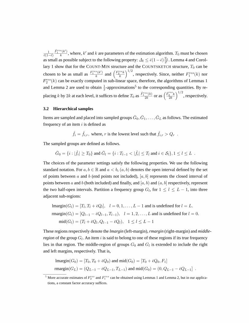
1ε(1−ε)
F res1 (k′)
k , where,k′ andk are parameters of the estimation algorithm.T0 must be chosen
as small as possible subject to the following property:∆l ≤ ε(1− ε)T0
2l . Lemma 4 and Corol-
lary 1 show that for the COUNT-M IN structure and the COUNTSKETCHstructure,T0 can be
chosen to be as small asFres1 (k′)
k and(
Fres2 kk
)1/2, respectively. Since, neitherF res
1 (k) nor
Fres2 (k) can be exactly computed in sub-linear space, therefore, the algorithms of Lemmas 1
and Lemma 2 are used to obtain12 -approximations5 to the corresponding quantities. By re-
placingk by 2k at each level, it suffices to defineT0 as F res1 (k)2k or as
(F
res2 k2k
)1/2, respectively.
3.2 Hierarchical samples
Items are sampled and placed into sampled groupsG0, G1, . . . , GL as follows. The estimated
frequency of an itemi is defined as
fi = fi,r, where,r is the lowest level such thatfi,r > Qr .
The sampled groups are defined as follows.
G0 = i : |fi| ≥ T0 andGl = i : Tl−1 < |fi| ≤ Tl andi ∈ Sl, 1 ≤ l ≤ L .
The choices of the parameter settings satisfy the following properties. We use the following
standard notation. Fora, b ∈ R anda < b, (a, b) denotes the open interval defined by the set
of points betweena andb (end points not included),[a, b] represents the closed interval of
points betweena andb (both included) and finally, and[a, b) and(a, b] respectively, represent
the two half-open intervals. Partition a frequency groupGl, for 1 ≤ l ≤ L − 1, into three
adjacent sub-regions:
lmargin(Gl) = [Tl, Tl + εQl], l = 0, 1, . . . , L− 1 and is undefined forl = L.
rmargin(Gl) = [Ql−1 − εQl−1, Tl−1), l = 1, 2, . . . , L and is undefined forl = 0.
mid(Gl) = (Tl + εQl, Ql−1 − εQl), 1 ≤ l ≤ L− 1
These regions respectively denote thelmargin(left-margin),rmargin(right-margin) andmiddle-
regionof the groupGl. An itemi is said to belong to one of these regions if its true frequency
lies in that region. The middle-region of groupsG0 andGl is extended to include the right
and left margins, respectively. That is,
lmargin(G0) = [T0, T0 + εQ0) and mid(G0) = [T0 + εQ0, F1]
rmargin(GL) = (QL−1 − εQL−1, TL−1) and mid(G0) = (0, QL−1 − εQL−1] .
5 More accurate estimates ofFres2 andF res
1 can be obtained using Lemmas 1 and Lemma 2, but in our applica-
tions, a constant factor accuracy suffices.

Important Convention. For clarity of presentation, from now on, the description of the
algorithm and the analysis throughout uses the frequenciesfi instead of|fi|. However, the
analysis remains unchanged if the frequencies are negative and|fi| is used in terms offi.
The only reason for making this notational convenience is to avoid writing|·| in many places.
An equivalent way of viewing this is to assume that the actual frequencies are given by an
n-dimensional vectorg. The vectorf is defined as the absolute value ofg, taken coordinate
wise, (i.e.,fi = |gi| for all i). It is important to note that the HSS technique is only designed
to work with functions of the form∑n
i=1 ψ(|gi|). All results in this paper and their analysis,
hold for general update data streams, where, item frequencies could be positive, negative or
zero.
We would now like to show that the following properties hold, with probability1− 2−t each.
1. Items belonging to the middle region of anyGl may be discovered as frequent, that is,
fi,r ≥ Qr, only at a levelr ≥ l. Further,fi = fi,l, that is, the estimate of its frequency
is obtained from levell. These items are never misclassified, that is, ifi belongs to some
sampled groupGr, then,r = l.
2. Items belonging to the right region ofGl may be discovered as frequent at levelr ≥ l−1,
but not at levels less thanl − 1, for l ≥ 1. Such items may be misclassified, but only to
the extent thati may be placed in eitherGl−1 or Gl.
3. Similarly, items belonging to the left-region ofGl may be discovered as frequent only at
levelsl or higher. Such items may be misclassified, but only to the extent thati is placed
either inGl or in Gl+1.
Lemma 5 states the properties formally.
Lemma 5. Let ε ≤ 16 . The following properties hold conditional on the eventGOODEST.
1. Supposei ∈ mid(Gl). Then,i is classified intoGl iff i ∈ Sl and fi = fi,l. If i 6∈ Sl, then,
fi is undefined andi is unclassified.
2. Supposei ∈ lmargin(Gl), for somel ∈ 0, 1, . . . , L−1. If i 6∈ Sl, then,i is not classified
into any group. Supposei ∈ Sl. Then, (1)i is classified intoGl iff i ∈ Sl and fi,l ≥ Tl,
and, (2)i is classified intoGl+1 iff i ∈ Sl+1 fi,l < Tl. In both cases,fi = fi,l.
3. Supposei ∈ rmargin(Gl) for some somel ∈ 1, 2, . . . , L. If i 6∈ Sl−1, then, fi is
undefined andi is unclassified. Supposei ∈ Sl−1. Then,
(a) i is classified intoGl−1 iff (1) fi,l−1 ≥ Tl−1, or, (2) fi,l−1 < Ql and i ∈ Sl and
fi,l ≥ Tl−1. In case (1),fi = fi,l−1 and in case (2),fi = fi,l.
(b) i is classified intoGl iff i ∈ Sl and either (1)fi,l−1 ≥ Ql−1 and fi < Tl−1, or, (2)
fi,l−1 < Ql−1 and fi = fi,l. In case (1),fi = fi,l−1 and in case (2)fi = fi,l.
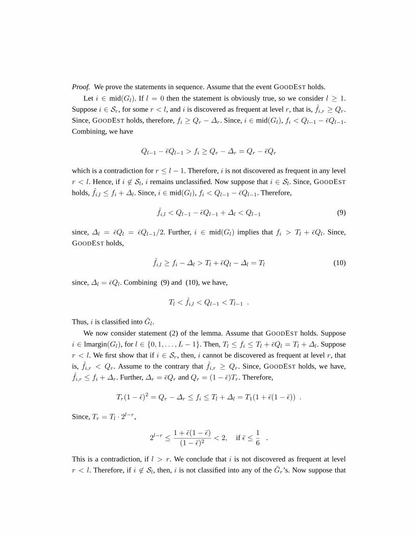
Proof. We prove the statements in sequence. Assume that the event GOODEST holds.
Let i ∈ mid(Gl). If l = 0 then the statement is obviously true, so we considerl ≥ 1.
Supposei ∈ Sr, for somer < l, andi is discovered as frequent at levelr, that is,fi,r ≥ Qr.
Since, GOODEST holds, therefore,fi ≥ Qr −∆r. Since,i ∈ mid(Gl), fi < Ql−1 − εQl−1.
Combining, we have
Ql−1 − εQl−1 > fi ≥ Qr −∆r = Qr − εQr
which is a contradiction forr ≤ l − 1. Therefore,i is not discovered as frequent in any level
r < l. Hence, ifi 6∈ Sl, i remains unclassified. Now suppose thati ∈ Sl. Since, GOODEST
holds,fi,l ≤ fi +∆l. Since,i ∈ mid(Gl), fi < Ql−1 − εQl−1. Therefore,
fi,l < Ql−1 − εQl−1 +∆l < Ql−1 (9)
since,∆l = εQl = εQl−1/2. Further,i ∈ mid(Gl) implies thatfi > Tl + εQl. Since,
GOODEST holds,
fi,l ≥ fi −∆l > Tl + εQl −∆l = Tl (10)
since,∆l = εQl. Combining (9) and (10), we have,
Tl < fi,l < Ql−1 < Tl−1 .
Thus,i is classified intoGl.
We now consider statement (2) of the lemma. Assume that GOODEST holds. Suppose
i ∈ lmargin(Gl), for l ∈ 0, 1, . . . , L − 1. Then,Tl ≤ fi ≤ Tl + εQl = Tl +∆l. Suppose
r < l. We first show that ifi ∈ Sr, then,i cannot be discovered as frequent at levelr, that
is, fi,r < Qr. Assume to the contrary thatfi,r ≥ Qr. Since, GOODEST holds, we have,
fi,r ≤ fi +∆r. Further,∆r = εQr andQr = (1− ε)Tr. Therefore,
Tr(1− ε)2 = Qr −∆r ≤ fi ≤ Tl +∆l = T1(1 + ε(1− ε)) .
Since,Tr = Tl · 2l−r,
2l−r ≤ 1 + ε(1− ε)(1− ε)2
< 2, if ε ≤ 16
.
This is a contradiction, ifl > r. We conclude thati is not discovered as frequent at level
r < l. Therefore, ifi 6∈ Sl, then,i is not classified into any of theGr ’s. Now suppose that
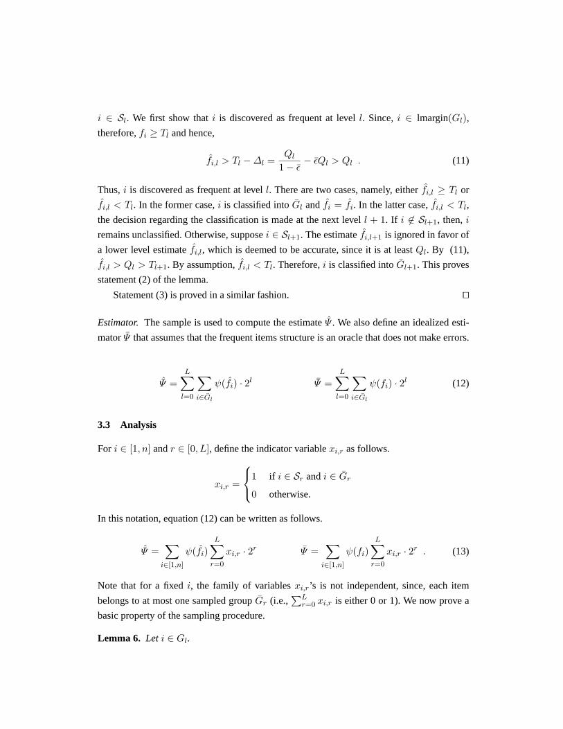
i ∈ Sl. We first show thati is discovered as frequent at levell. Since,i ∈ lmargin(Gl),therefore,fi ≥ Tl and hence,
fi,l > Tl −∆l =Ql
1− ε− εQl > Ql . (11)
Thus,i is discovered as frequent at levell. There are two cases, namely, eitherfi,l ≥ Tl or
fi,l < Tl. In the former case,i is classified intoGl andfi = fi. In the latter case,fi,l < Tl,
the decision regarding the classification is made at the next levell + 1. If i 6∈ Sl+1, then,i
remains unclassified. Otherwise, supposei ∈ Sl+1. The estimatefi,l+1 is ignored in favor of
a lower level estimatefi,l, which is deemed to be accurate, since it is at leastQl. By (11),
fi,l > Ql > Tl+1. By assumption,fi,l < Tl. Therefore,i is classified intoGl+1. This proves
statement (2) of the lemma.
Statement (3) is proved in a similar fashion. ut
Estimator. The sample is used to compute the estimateΨ . We also define an idealized esti-
matorΨ that assumes that the frequent items structure is an oracle that does not make errors.
Ψ =L∑
l=0
∑i∈Gl
ψ(fi) · 2l Ψ =L∑
l=0
∑i∈Gl
ψ(fi) · 2l (12)
3.3 Analysis
For i ∈ [1, n] andr ∈ [0, L], define the indicator variablexi,r as follows.
xi,r =
1 if i ∈ Sr andi ∈ Gr
0 otherwise.
In this notation, equation (12) can be written as follows.
Ψ =∑
i∈[1,n]
ψ(fi)L∑
r=0
xi,r · 2r Ψ =∑
i∈[1,n]
ψ(fi)L∑
r=0
xi,r · 2r . (13)
Note that for a fixedi, the family of variablesxi,r ’s is not independent, since, each item
belongs to at most one sampled groupGr (i.e.,∑L
r=0 xi,r is either 0 or 1). We now prove a
basic property of the sampling procedure.
Lemma 6. Let i ∈ Gl.
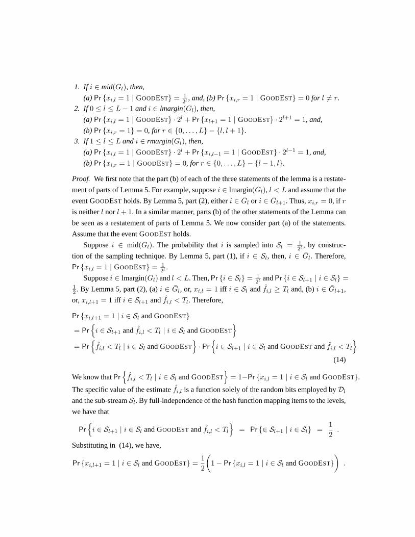
1. If i ∈ mid(Gl), then,
(a) Pr xi,l = 1 | GOODEST = 12l , and, (b)Pr xi,r = 1 | GOODEST = 0 for l 6= r.
2. If 0 ≤ l ≤ L− 1 andi ∈ lmargin(Gl), then,
(a) Pr xi,l = 1 | GOODEST · 2l + Pr xl+1 = 1 | GOODEST · 2l+1 = 1, and,
(b) Pr xi,r = 1 = 0, for r ∈ 0, . . . , L − l, l + 1.3. If 1 ≤ l ≤ L andi ∈ rmargin(Gl), then,
(a) Pr xi,l = 1 | GOODEST · 2l + Pr xi,l−1 = 1 | GOODEST · 2l−1 = 1, and,
(b) Pr xi,r = 1 | GOODEST = 0, for r ∈ 0, . . . , L − l − 1, l.
Proof. We first note that the part (b) of each of the three statements of the lemma is a restate-
ment of parts of Lemma 5. For example, supposei ∈ lmargin(Gl), l < L and assume that the
event GOODEST holds. By Lemma 5, part (2), eitheri ∈ Gl or i ∈ Gl+1. Thus,xi,r = 0, if r
is neitherl nor l+ 1. In a similar manner, parts (b) of the other statements of the Lemma can
be seen as a restatement of parts of Lemma 5. We now consider part (a) of the statements.
Assume that the event GOODEST holds.
Supposei ∈ mid(Gl). The probability thati is sampled intoSl = 12l , by construc-
tion of the sampling technique. By Lemma 5, part (1), ifi ∈ Sl, then,i ∈ Gl. Therefore,
Pr xi,l = 1 | GOODEST = 12l .
Supposei ∈ lmargin(Gl) andl < L. Then,Pr i ∈ Sl = 12l andPr i ∈ Sl+1 | i ∈ Sl =
12 . By Lemma 5, part (2), (a)i ∈ Gl, or,xi,l = 1 iff i ∈ Sl andfi,l ≥ Tl and, (b)i ∈ Gl+1,
or,xi,l+1 = 1 iff i ∈ Sl+1 andfi,l < Tl. Therefore,
Pr xi,l+1 = 1 | i ∈ Sl and GOODEST
= Pri ∈ Sl+1 andfi,l < Tl | i ∈ Sl and GOODEST
= Pr
fi,l < Tl | i ∈ Sl and GOODEST
· Pr
i ∈ Sl+1 | i ∈ Sl and GOODEST andfi,l < Tl
(14)
We know thatPrfi,l < Tl | i ∈ Sl and GOODEST
= 1−Pr xi,l = 1 | i ∈ Sl and GOODEST.
The specific value of the estimatefi,l is a function solely of the random bits employed byDl
and the sub-streamSl. By full-independence of the hash function mapping items to the levels,
we have that
Pri ∈ Sl+1 | i ∈ Sl and GOODEST andfi,l < Tl
= Pr ∈ Sl+1 | i ∈ Sl =
12.
Substituting in (14), we have,
Pr xi,l+1 = 1 | i ∈ Sl and GOODEST =12
(1− Pr xi,l = 1 | i ∈ Sl and GOODEST
).
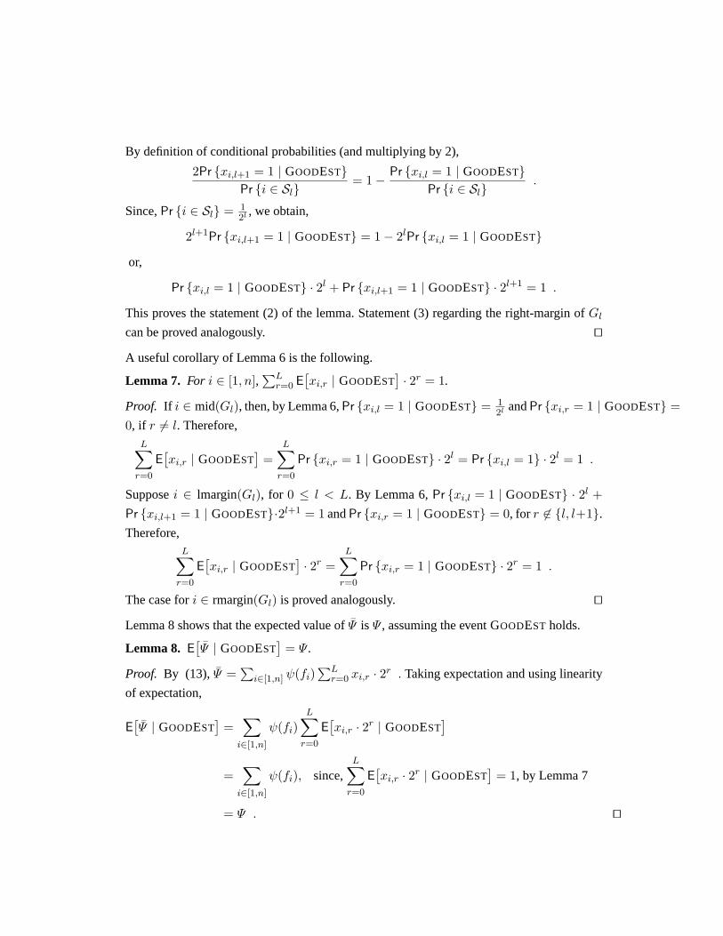
By definition of conditional probabilities (and multiplying by 2),
2Pr xi,l+1 = 1 | GOODESTPr i ∈ Sl
= 1−Pr xi,l = 1 | GOODEST
Pr i ∈ Sl.
Since,Pr i ∈ Sl = 12l , we obtain,
2l+1Pr xi,l+1 = 1 | GOODEST = 1− 2lPr xi,l = 1 | GOODEST
or,
Pr xi,l = 1 | GOODEST · 2l + Pr xi,l+1 = 1 | GOODEST · 2l+1 = 1 .
This proves the statement (2) of the lemma. Statement (3) regarding the right-margin ofGl
can be proved analogously. ut
A useful corollary of Lemma 6 is the following.
Lemma 7. For i ∈ [1, n],∑L
r=0 E[xi,r | GOODEST
]· 2r = 1.
Proof. If i ∈ mid(Gl), then, by Lemma 6,Pr xi,l = 1 | GOODEST = 12l andPr xi,r = 1 | GOODEST =
0, if r 6= l. Therefore,L∑
r=0
E[xi,r | GOODEST
]=
L∑r=0
Pr xi,r = 1 | GOODEST · 2l = Pr xi,l = 1 · 2l = 1 .
Supposei ∈ lmargin(Gl), for 0 ≤ l < L. By Lemma 6,Pr xi,l = 1 | GOODEST · 2l +Pr xi,l+1 = 1 | GOODEST·2l+1 = 1 andPr xi,r = 1 | GOODEST = 0, for r 6∈ l, l+1.Therefore,
L∑r=0
E[xi,r | GOODEST
]· 2r =
L∑r=0
Pr xi,r = 1 | GOODEST · 2r = 1 .
The case fori ∈ rmargin(Gl) is proved analogously. ut
Lemma 8 shows that the expected value ofΨ is Ψ , assuming the event GOODEST holds.
Lemma 8. E[Ψ | GOODEST
]= Ψ .
Proof. By (13), Ψ =∑
i∈[1,n] ψ(fi)∑L
r=0 xi,r · 2r . Taking expectation and using linearity
of expectation,
E[Ψ | GOODEST
]=∑
i∈[1,n]
ψ(fi)L∑
r=0
E[xi,r · 2r | GOODEST
]=∑
i∈[1,n]
ψ(fi), since,L∑
r=0
E[xi,r · 2r | GOODEST
]= 1, by Lemma 7
= Ψ . ut

The following lemma is useful in the calculation of the variance ofΨ .
Notation.Let l(i) denote the index of the groupGl such thati ∈ Gl.
Lemma 9. For i ∈ [1, n] and i 6∈ G0 − lmargin(G0),∑L
r=0 E[xi,r · 22r | GOODEST
]≤
2l(i)+1. If i ∈ G0 − lmargin(G0), then,∑L
r=0 E[xi,r · 22r | GOODEST
]= 1.
Proof. We assume that all probabilities and expectations in this proof are conditioned on the
event GOODEST. For brevity, we do not write the conditioning event. Leti ∈ mid(Gl) and
assume that GOODEST holds. Then,xi,l = 1 iff i ∈ Sl, by Lemma 6. Thus,
Pr xi,l = 1 · 22l =12l· 22l = 2l .
If i ∈ lmargin(Gl), then, by the argument in Lemma 7,
Pr xi,l+1 = 1 · 2l+1 + Pr xi,l = 1 · 2l = 1 .
Multiplying by 2l+1,
Pr xi,l+1 = 1 22(l+1) + Pr xi,l = 1 22l ≤ 2l+1 .
Similarly, if i ∈ rmargin(Gl), then,
Pr xi,l = 1 2l + Pr xi,l−1 = 1 2l−1 = 1 .
Therefore,
Pr xi,l = 1 22l + Pr xi,l−1 = 1 22(l−1) ≤ 22l
Since,l(i) denotes the index of the groupGl to whichi belongs, therefore,
L∑r=0
E[xi,r · 22r
]< 2l(i)+1 .
In particular, ifi ∈ G0 − lmargin(G0) or if i ∈ mid(Gl), then, the above sum is2l(i). ut
Lemma 10.
Var[Ψ | GOODEST
]≤
∑i∈[1,n]
i/∈(G0−lmargin(G0))
ψ2(fi) · 2l(i)+1 .
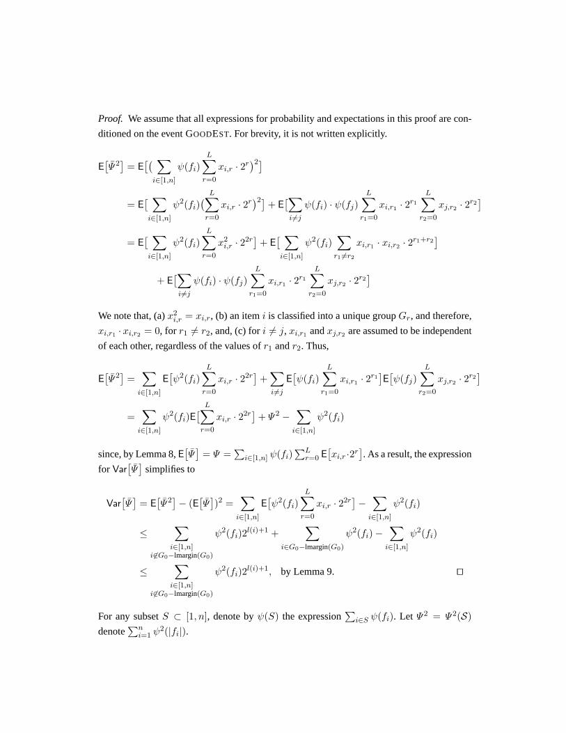
Proof. We assume that all expressions for probability and expectations in this proof are con-
ditioned on the event GOODEST. For brevity, it is not written explicitly.
E[Ψ2]
= E[( ∑
i∈[1,n]
ψ(fi)L∑
r=0
xi,r · 2r)2]
= E[ ∑i∈[1,n]
ψ2(fi)( L∑
r=0
xi,r · 2r)2]+ E
[∑i6=j
ψ(fi) · ψ(fj)L∑
r1=0
xi,r1 · 2r1
L∑r2=0
xj,r2 · 2r2]
= E[ ∑i∈[1,n]
ψ2(fi)L∑
r=0
x2i,r · 22r
]+ E
[ ∑i∈[1,n]
ψ2(fi)∑
r1 6=r2
xi,r1 · xi,r2 · 2r1+r2]
+ E[∑
i6=j
ψ(fi) · ψ(fj)L∑
r1=0
xi,r1 · 2r1
L∑r2=0
xj,r2 · 2r2]
We note that, (a)x2i,r = xi,r, (b) an itemi is classified into a unique groupGr, and therefore,
xi,r1 · xi,r2 = 0, for r1 6= r2, and, (c) fori 6= j, xi,r1 andxj,r2 are assumed to be independent
of each other, regardless of the values ofr1 andr2. Thus,
E[Ψ2]
=∑
i∈[1,n]
E[ψ2(fi)
L∑r=0
xi,r · 22r]+∑i6=j
E[ψ(fi)
L∑r1=0
xi,r1 · 2r1]E[ψ(fj)
L∑r2=0
xj,r2 · 2r2]
=∑
i∈[1,n]
ψ2(fi)E[ L∑r=0
xi,r · 22r]+ Ψ2 −
∑i∈[1,n]
ψ2(fi)
since, by Lemma 8,E[Ψ]
= Ψ =∑
i∈[1,n] ψ(fi)∑L
r=0 E[xi,r ·2r
]. As a result, the expression
for Var[Ψ]
simplifies to
Var[Ψ]
= E[Ψ2]− (E
[Ψ])2 =
∑i∈[1,n]
E[ψ2(fi)
L∑r=0
xi,r · 22r]−∑
i∈[1,n]
ψ2(fi)
≤∑
i∈[1,n]i6∈G0−lmargin(G0)
ψ2(fi)2l(i)+1 +∑
i∈G0−lmargin(G0)
ψ2(fi)−∑
i∈[1,n]
ψ2(fi)
≤∑
i∈[1,n]i6∈G0−lmargin(G0)
ψ2(fi)2l(i)+1, by Lemma 9. ut
For any subsetS ⊂ [1, n], denote byψ(S) the expression∑
i∈S ψ(fi). Let Ψ2 = Ψ2(S)denote
∑ni=1 ψ
2(|fi|).

Corollary 2. If the functionψ(·) is non-decreasing in the interval[0 . . . T0 +∆0], then,
Var[Ψ | GOODEST
]=
L∑l=1
ψ(Tl−1)ψ(Gl)2l+1 + ψ(T0 +∆0)ψ(lmargin(G0)) (15)
Proof. If the monotonicity condition is satisfied, thenψ(Tl−1) ≥ ψ(fi) for all i ∈ Gl, l ≥ 1andψ(fi) ≤ ψ(T0 +∆0) for i ∈ lmargin(G0). Therefore,ψ2(fi) ≤ ψ(Tl−1) · ψ(fi), in the
first case andψ2(fi) ≤ ψ(T0 +∆0) in the second case. By Lemma 10,
Var[Ψ | GOODEST
]≤
L∑l=1
∑i∈Gl
ψ(Tl−1)ψ(fi)2l(i)+1 +∑
i∈lmargin(G0)
ψ(T0 +∆0)ψ(fi)
=L∑
l=1
ψ(Tl−1)ψ(Gl)2l+1 + ψ(T0 +∆0)ψ(lmargin(G0)) . ut
3.4 Error in the estimate
The error incurred by our estimateΨ is |Ψ − Ψ |, and can be written as the sum of two error
components using triangle inequality.
|Ψ − Ψ | ≤ |Ψ − Ψ |+ |Ψ − Ψ | = E1 + E2
Here,E1 = |Ψ − Ψ | is the error due to sampling andE2 = |Ψ − Ψ | is the error due to the
estimation of the frequencies. By Chebychev’s inequality
PrE1 ≤ 3(Var
[Ψ])1/2 | GOODEST
≥ 8
9.
Substituting the expression forVar[Ψ]
from (15),
Pr
E1 ≤ 3
( L∑l=1
ψ(Tl−1)ψ(Gl)2l+1 + ψ(T0 +∆0)ψ(lmargin(G0)))1/2∣∣∣∣GOODEST
≥ 89. (16)
We now present an upper bound onE2. Define a real valued functionπ : [1, n] → R as
follows.
πi =
∆l · |ψ′(ξi(fi,∆l))| if i ∈ G0 − lmargin(G0) or i ∈ mid(Gl)
∆l · |ψ′(ξi(fi,∆l))| if i ∈ lmargin(Gl), for somel > 1
∆l−1 · |ψ′(ξi(fi,∆l−1))| if i ∈ rmargin(Gl)
where, the notationξi(fi,∆l) returns the value oft that maximizes|ψ′(t)| in the interval
[fi −∆l, fi +∆l].
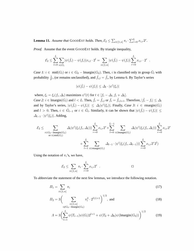
Lemma 11. Assume thatGOODEST holds. Then,E2 ≤∑
i∈[1,n] πi ·∑L
r=0 xi,r2r.
Proof. Assume that the event GOODEST holds. By triangle inequality,
E2 ≤L∑
l=0
∑i∈Gl
|ψ(fi)− ψ(fi)|xi,l · 2l =∑
i∈[1,n]
|ψ(fi)− ψ(fi)|L∑
r=0
xi,r · 2r .
Case 1:i ∈ mid(Gl) or i ∈ G0 − lmargin(G0). Then,i is classified only in groupGl with
probability 12l , (or remains unclassified), andfi,l = fi, by Lemma 6. By Taylor’s series
|ψ(fi)− ψ(fi)| ≤ ∆l · |ψ′(ξi)|
where,ξi = ξi(fi,∆l) maximizesψ′(t) for t ∈ [fi −∆l, fi +∆l].Case 2:i ∈ lmargin(Gl) andl < L. Then,fi = fi,l or fi = fi,l+1. Therefore,|fi − fi| ≤ ∆l
and by Taylor’s series,|ψ(fi)− ψ(fi)| ≤ ∆l|ψ′(ξi)|. Finally, Case 3:i ∈ rmargin(Gl)and l > 0. Then,i ∈ Gl−1 or i ∈ Gl. Similarly, it can be shown that|ψ(fi)− ψ(fi)| ≤∆l−1 · |ψ′(ξi)|. Adding,
E2 ≤∑
i∈G0−lmargin(G0)or i∈mid(Gl)
∆l|ψ′(ξi(fi,∆l))|L∑
r=0
xi,r2r+L−1∑l=0
∑i∈lmargin(Gl)
∆l|ψ′(ξi(fi,∆l))|L∑
r=0
xi,r2r
+L∑
l=1
∑i∈rmargin(Gl)
∆l−1 · |ψ′(ξi(fi,∆l−1))|L∑
r=0
xi,r2r2l)
Using the notation ofπi’s, we have,
E2 ≤∑
i∈[1,n]
πi ·L∑
r=0
xi,r2r . ut
To abbreviate the statement of the next few lemmas, we introduce the following notation.
Π1 =∑
i∈[1,n]
πi (17)
Π2 = 3( ∑
i∈[1,n]i6∈G0−lmargin(G0)
π2i · 2l(i)+1
)1/2
, and (18)
Λ = 3( L∑
l=1
ψ(Tl−1)ψ(Gl)2l+1 + ψ(T0 +∆0)ψ(lmargin(G0)))1/2
(19)
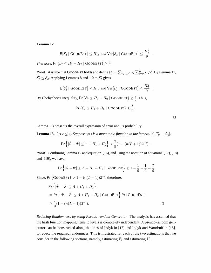
Lemma 12.
E[E2 | GOODEST
]≤ Π1, andVar
[E2 | GOODEST
]≤ Π2
2
9.
Therefore,Pr E2 ≤ Π1 +Π2 | GOODEST ≥ 89 .
Proof. Assume that GOODEST holds and defineE ′2 =∑
i∈[1,n] πi∑L
l=0 xi,l2l. By Lemma 11,
E ′2 ≤ E2. Applying Lemmas 8 and 10 toE ′2 gives
E[E ′2 | GOODEST
]≤ Π1, andVar
[E ′2 | GOODEST
]≤ Π2
2
9.
By Chebychev’s inequality,Pr E ′2 ≤ Π1 +Π2 | GOODEST ≥ 89 . Thus,
Pr E2 ≤ Π1 +Π2 | GOODEST ≥ 89.
ut
Lemma 13 presents the overall expression of error and its probability.
Lemma 13. Let ε ≤ 13 . Supposeψ() is a monotonic function in the interval[0, T0 +∆0].
Pr|Ψ − Ψ | ≤ Λ+Π1 +Π2
>
79(1− (n(L+ 1))2−t) .
Proof. Combining Lemma 12 and equation (16), and using the notation of equations (17), (18)
and (19), we have,
Pr|Ψ − Ψ | ≤ Λ+Π1 +Π2 | GOODEST
≥ 1− 1
9− 1
9=
79
Since,Pr GOODEST > 1− (n(L+ 1))2−t, therefore,
Pr|Ψ − Ψ | ≤ Λ+Π1 +Π2
= Pr
|Ψ − Ψ | ≤ Λ+Π1 +Π2 | GOODEST
Pr GOODEST
≥ 79(1− (n(L+ 1))2−t). ut
Reducing Randomness by using Pseudo-random Generator.The analysis has assumed that
the hash function mapping items to levels is completely independent. A pseudo-random gen-
erator can be constructed along the lines of Indyk in [17] and Indyk and Woodruff in [18],
to reduce the required randomness. This is illustrated for each of the two estimations that we
consider in the following sections, namely, estimatingFp and estimatingH.
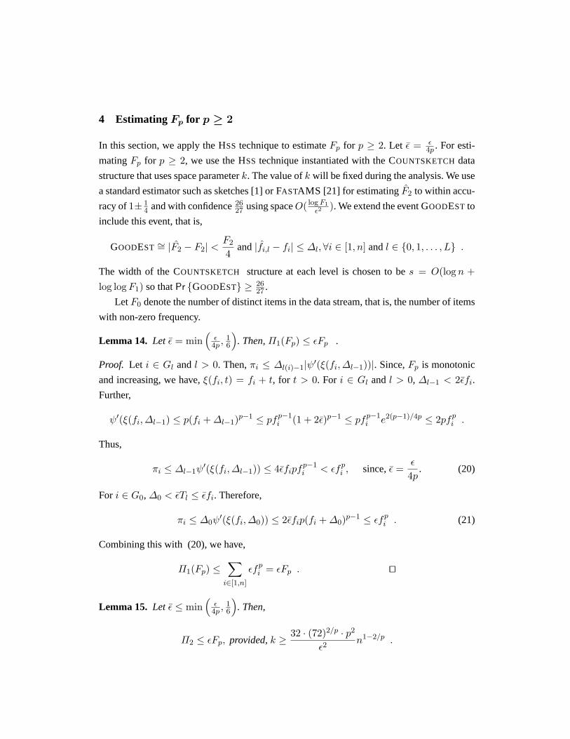
4 Estimating Fp for p ≥ 2
In this section, we apply the HSS technique to estimateFp for p ≥ 2. Let ε = ε4p . For esti-
matingFp for p ≥ 2, we use the HSS technique instantiated with the COUNTSKETCH data
structure that uses space parameterk. The value ofk will be fixed during the analysis. We use
a standard estimator such as sketches [1] or FASTAMS [21] for estimatingF2 to within accu-
racy of1± 14 and with confidence2627 using spaceO( log F1
ε2). We extend the event GOODEST to
include this event, that is,
GOODEST∼= |F2 − F2| <F2
4and|fi,l − fi| ≤ ∆l,∀i ∈ [1, n] andl ∈ 0, 1, . . . , L .
The width of the COUNTSKETCH structure at each level is chosen to bes = O(log n +log logF1) so thatPr GOODEST ≥ 26
27 .
LetF0 denote the number of distinct items in the data stream, that is, the number of items
with non-zero frequency.
Lemma 14. Let ε = min(
ε4p ,
16
). Then,Π1(Fp) ≤ εFp .
Proof. Let i ∈ Gl andl > 0. Then,πi ≤ ∆l(i)−1|ψ′(ξ(fi,∆l−1))|. Since,Fp is monotonic
and increasing, we have,ξ(fi, t) = fi + t, for t > 0. For i ∈ Gl andl > 0, ∆l−1 < 2εfi.
Further,
ψ′(ξ(fi,∆l−1) ≤ p(fi +∆l−1)p−1 ≤ pfp−1i (1 + 2ε)p−1 ≤ pfp−1
i e2(p−1)/4p ≤ 2pfpi .
Thus,
πi ≤ ∆l−1ψ′(ξ(fi,∆l−1)) ≤ 4εfipf
p−1i < εfp
i , since,ε =ε
4p. (20)
For i ∈ G0,∆0 < εTl ≤ εfi. Therefore,
πi ≤ ∆0ψ′(ξ(fi,∆0)) ≤ 2εfip(fi +∆0)p−1 ≤ εfp
i . (21)
Combining this with (20), we have,
Π1(Fp) ≤∑
i∈[1,n]
εfpi = εFp . ut
Lemma 15. Let ε ≤ min(
ε4p ,
16
). Then,
Π2 ≤ εFp, provided,k ≥ 32 · (72)2/p · p2
ε2n1−2/p .
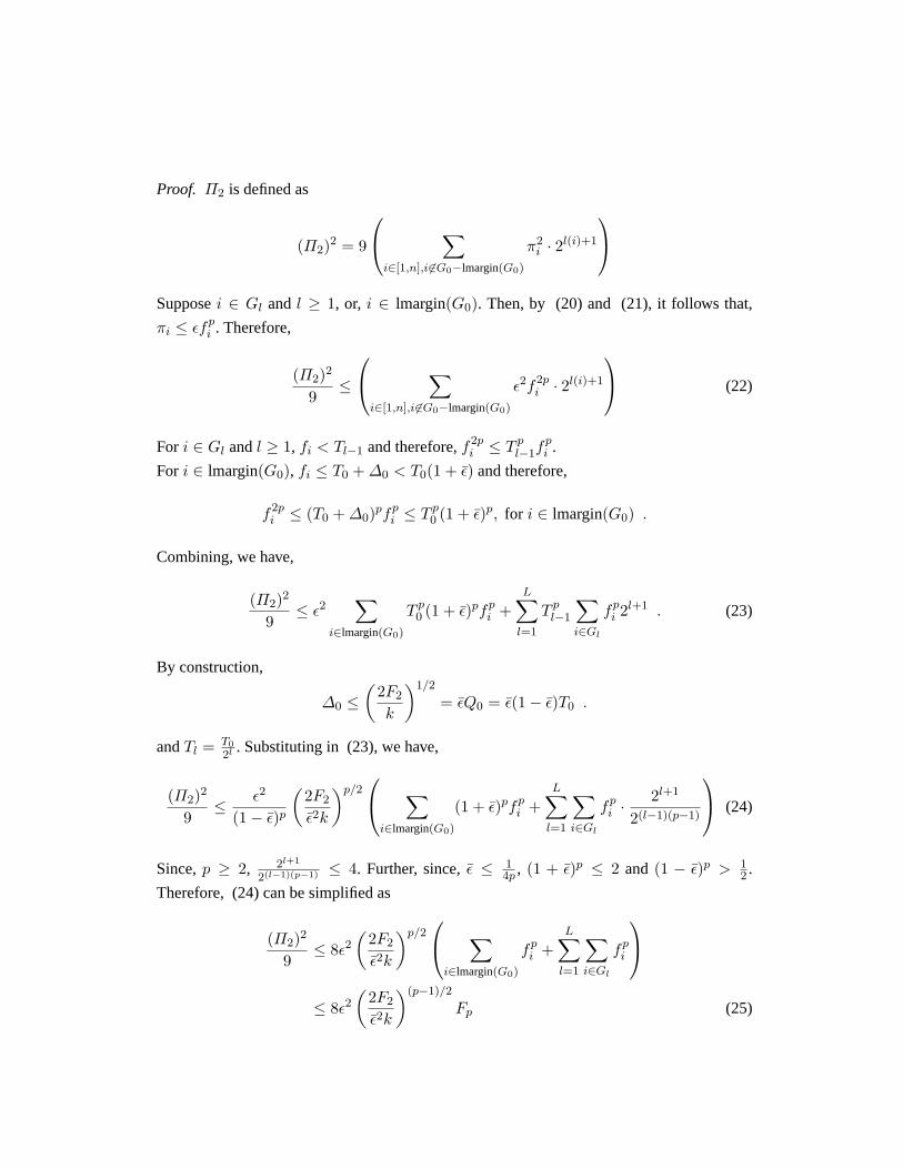
Proof. Π2 is defined as
(Π2)2 = 9
∑i∈[1,n],i6∈G0−lmargin(G0)
π2i · 2l(i)+1
Supposei ∈ Gl and l ≥ 1, or, i ∈ lmargin(G0). Then, by (20) and (21), it follows that,
πi ≤ εfpi . Therefore,
(Π2)2
9≤
∑i∈[1,n],i6∈G0−lmargin(G0)
ε2f2pi · 2l(i)+1
(22)
For i ∈ Gl andl ≥ 1, fi < Tl−1 and therefore,f2pi ≤ T p
l−1fpi .
For i ∈ lmargin(G0), fi ≤ T0 +∆0 < T0(1 + ε) and therefore,
f2pi ≤ (T0 +∆0)pfp
i ≤ T p0 (1 + ε)p, for i ∈ lmargin(G0) .
Combining, we have,
(Π2)2
9≤ ε2
∑i∈lmargin(G0)
T p0 (1 + ε)pfp
i +L∑
l=1
T pl−1
∑i∈Gl
fpi 2l+1 . (23)
By construction,
∆0 ≤(
2F2
k
)1/2
= εQ0 = ε(1− ε)T0 .
andTl = T0
2l . Substituting in (23), we have,
(Π2)2
9≤ ε2
(1− ε)p
(2F2
ε2k
)p/2 ∑
i∈lmargin(G0)
(1 + ε)pfpi +
L∑l=1
∑i∈Gl
fpi ·
2l+1
2(l−1)(p−1)
(24)
Since,p ≥ 2, 2l+1
2(l−1)(p−1) ≤ 4. Further, since,ε ≤ 14p , (1 + ε)p ≤ 2 and (1 − ε)p > 1
2 .
Therefore, (24) can be simplified as
(Π2)2
9≤ 8ε2
(2F2
ε2k
)p/2 ∑
i∈lmargin(G0)
fpi +
L∑l=1
∑i∈Gl
fpi
≤ 8ε2
(2F2
ε2k
)(p−1)/2
Fp (25)

since,(∑
i∈lmargin(G0) fpi +
∑Ll=1
∑i∈Gl
fpi
)= Fp−
∑i∈G0−lmargin(G0) f
pi . We now use the
identity (F2
F0
)1/2
≤(Fr
F0
)1/r
or,F r/22 ≤ Fr · F r/2−1
0 , for anyr ≥ 2 . (26)
Letting r = p, we haveF p2 < FpF
p/2−10 . Substituting in (25), we have,
(Π2)2 ≤72 · 2p/2 · ε2 · F 2
p · Fp/2−10
(ε2k)p/2· Fp ≤ 72ε2 · 2p/2 · F 2
p
(n1−2/p
ε2k
)p/2
Lettingk = 2·(72)2/p
ε2n1−2/p = 32·(72)2/p·p2
ε2n1−2/p, we have,
(Π2)2 ≤ ε2F 2p , or,Π2 ≤ εFp . ut
Lemma 16.
If ε ≤ min(ε
4p,16
)andk ≥ 32 · (72)2/p · p2
ε2+4/pn1−2/p, then,Λ < εFp .
Proof. The expression (19) forΛ can be written as follows.
Λ2
9=
∑i∈lmargin(G0)
(T0 +∆0)pfpi +
L∑l=1
(Tl−1)p∑i∈Gl
fpi 2l+1
(27)
Except for the factor ofε2, the expression on theRHSis identical to the expression in the
RHS (23), for which an upper bound was derived in Lemma 15. Following the same proof
and modifying the constants, we obtain that
Λ2 ≤ ε2F 2p if k ≥ 32 · (72)2/p · p2
ε2+4/pn1−2/p .
Recall thats is the width of the COUNTSKETCHstructures kept at each levell = 0, . . . , L.
Lemma 17. Supposep ≥ 2. Let k ≥ 32·(72)2/p·p2
ε2+4/p n1−2/p, ε = min(
ε4p ,
16
)and s =
O(log n+ log logF1) , then,Pr|Fp − Fp| < 3εFp
with probability 6
9 .
Proof. By Lemma 13,
Pr|Fp − Fp| ≤ Π1 +Π2 + Λ
≥ (1− 7
9)(Pr GOODEST) .
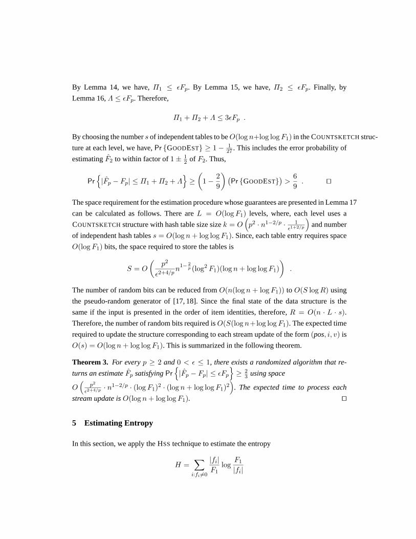
By Lemma 14, we have,Π1 ≤ εFp. By Lemma 15, we have,Π2 ≤ εFp. Finally, by
Lemma 16,Λ ≤ εFp. Therefore,
Π1 +Π2 + Λ ≤ 3εFp .
By choosing the numbers of independent tables to beO(log n+log logF1) in the COUNTSKETCHstruc-
ture at each level, we have,Pr GOODEST ≥ 1− 127 . This includes the error probability of
estimatingF2 to within factor of1± 12 of F2. Thus,
Pr|Fp − Fp| ≤ Π1 +Π2 + Λ
≥(
1− 29
)(Pr GOODEST
)>
69. ut
The space requirement for the estimation procedure whose guarantees are presented in Lemma 17
can be calculated as follows. There areL = O(logF1) levels, where, each level uses a
COUNTSKETCHstructure with hash table size sizek = O(p2 · n1−2/p · 1
ε1+2/p
)and number
of independent hash tabless = O(log n+ log logF1). Since, each table entry requires space
O(logF1) bits, the space required to store the tables is
S = O
(p2
ε2+4/pn
1− 2p (log2 F1)(log n+ log logF1)
).
The number of random bits can be reduced fromO(n(log n + logF1)) toO(S logR) using
the pseudo-random generator of [17, 18]. Since the final state of the data structure is the
same if the input is presented in the order of item identities, therefore,R = O(n · L · s).Therefore, the number of random bits required isO(S(log n+log logF1). The expected time
required to update the structure corresponding to each stream update of the form(pos, i, v) is
O(s) = O(log n+ log logF1). This is summarized in the following theorem.
Theorem 3. For everyp ≥ 2 and0 < ε ≤ 1, there exists a randomized algorithm that re-
turns an estimateFp satisfyingPr|Fp − Fp| ≤ εFp
≥ 2
3 using space
O(
p2
ε2+4/p · n1−2/p · (logF1)2 · (log n+ log logF1)2)
. The expected time to process each
stream update isO(log n+ log logF1). ut
5 Estimating Entropy
In this section, we apply the HSS technique to estimate the entropy
H =∑
i:fi 6=0
|fi|F1
logF1
|fi|
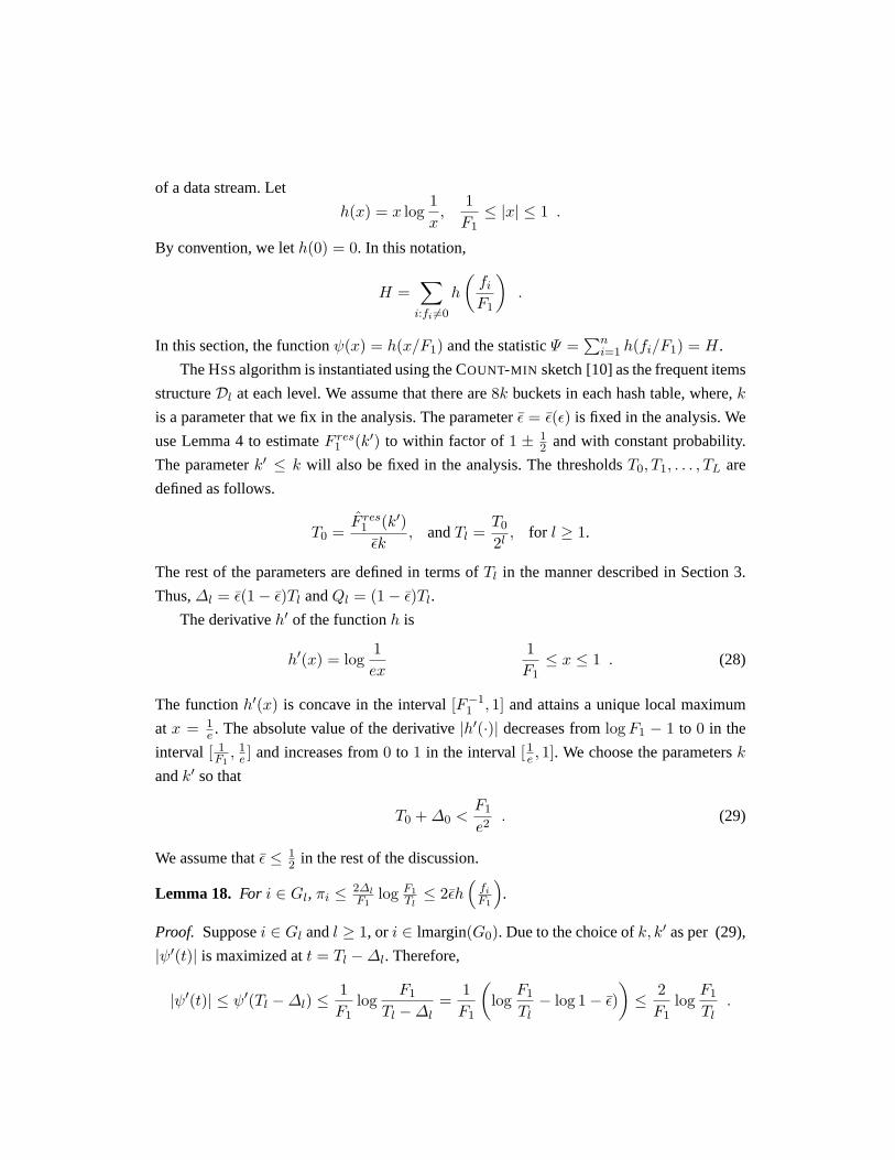
of a data stream. Let
h(x) = x log1x,
1F1
≤ |x| ≤ 1 .
By convention, we leth(0) = 0. In this notation,
H =∑
i:fi 6=0
h
(fi
F1
).
In this section, the functionψ(x) = h(x/F1) and the statisticΨ =∑n
i=1 h(fi/F1) = H.
The HSSalgorithm is instantiated using the COUNT-MIN sketch [10] as the frequent items
structureDl at each level. We assume that there are8k buckets in each hash table, where,k
is a parameter that we fix in the analysis. The parameterε = ε(ε) is fixed in the analysis. We
use Lemma 4 to estimateF res1 (k′) to within factor of1 ± 1
2 and with constant probability.
The parameterk′ ≤ k will also be fixed in the analysis. The thresholdsT0, T1, . . . , TL are
defined as follows.
T0 =F res
1 (k′)εk
, andTl =T0
2l, for l ≥ 1.
The rest of the parameters are defined in terms ofTl in the manner described in Section 3.
Thus,∆l = ε(1− ε)Tl andQl = (1− ε)Tl.
The derivativeh′ of the functionh is
h′(x) = log1ex
1F1
≤ x ≤ 1 . (28)
The functionh′(x) is concave in the interval[F−11 , 1] and attains a unique local maximum
at x = 1e . The absolute value of the derivative|h′(·)| decreases fromlogF1 − 1 to 0 in the
interval [ 1F1, 1
e ] and increases from0 to 1 in the interval[1e , 1]. We choose the parametersk
andk′ so that
T0 +∆0 <F1
e2. (29)
We assume thatε ≤ 12 in the rest of the discussion.
Lemma 18. For i ∈ Gl, πi ≤ 2∆lF1
log F1Tl≤ 2εh
(fi
F1
).
Proof. Supposei ∈ Gl andl ≥ 1, or i ∈ lmargin(G0). Due to the choice ofk, k′ as per (29),
|ψ′(t)| is maximized att = Tl −∆l. Therefore,
|ψ′(t)| ≤ ψ′(Tl −∆l) ≤1F1
logF1
Tl −∆l=
1F1
(log
F1
Tl− log 1− ε)
)≤ 2F1
logF1
Tl.

since,ε ≤ 12 , − log(1 − ε) ≤ log 2 = 1. Therefore,πi ≤ 2∆l
F1log F1
Tl. Further, fori ∈ Gl,
l ≥ 1 or, i ∈ lmargin(G0),
∆l
F1log
F1
Tl=εTl
Fllog
Fl
Tl< εh
(fi
F1
)Now supposei ∈ G0− lmargin(G0). Then, by (29),|ψ′(t)| has a maximum value att = T0.
Therefore,|ψ′(t)| ≤ 1F1
log F1T0
as explained above. The argument now proceeds in the same
manner as above. ut
Define the event GOODRESEST to beF res1 (k′) ≤ F res
1 (k′) ≤ 2F res1 (k′). By Lemma 2,
GOODRESEST holds with constant probability and can be accomplished using space
O (k′(logF1) + log n). We assume that the event GOODEST is broadened to include the
event GOODRESEST as well, such thatPr GOODEST ≥ 2627 .
Lemma 19. T0F1≤ 2H
εk(log k′) .
Proof. Since, GOODEST holds,T0 = F res1 (k′)
εk ≤ 2F res1 (k)εk . Therefore, if there are at mostk
distinct items in the stream (i.e.,F0 ≤ k), then,T0 = 0 and the lemma follows. Otherwise,
H ≥∑
rank(i)>k′
|fi|F1
logF1
fi≥
∑rank(i)>k′
|fi|F1
log k′ =log k′
F1F res
1 (k′) ≥ εk(log k′)T0
2F1. ut
Lemma 20. Π1 ≤ 2εH .
Proof. By definition,Π1 =∑
i∈[1,n] πi. By Lemma 18, we have,πi ≤ 2εh(
fi
F1
). Thus,
Π1 =∑
i∈[1,n]
πi ≤∑
i∈[1,n]
2εh(fi
F1
)= 2εH. ut
Lemma 21. Then,
Π22 ≤
36ε(log(2F1))H2
k(log k′).
Proof. By definition ofΠ2 (equation (18))
Π22
9=
L∑l=1
∑i∈Gl
π2i 2
l+1 +∑
i∈lmargin(G0)
π2i .
If F0 ≤ k′, then,F res1 (k′) = 0 and therefore,T0 = 0 and soΠ2 = 0¿ Therefore, without loss
of generality, we may assume thatF0 > k′. We first consider the summation over elements
in Gl, l ≥ 1. In this region,
|h′(fi/F1)| ≤ |h′(Tl/F1)| ≤1F1
logF1
eTl≤ 1F1
logF1
and therefore,
πi ≤ ∆l|h′(Tl/F1)| <εTl
F1logF1.
Further, by Lemma 18,πi ≤ 2εh(
fi
F1
). Therefore,
L∑l=1
∑i∈Gl
π2i 2
l+1 ≤L∑
l=1
∑i∈Gl
εTl
F1(logF1) · (2ε)h
(fi
F1
)· 2l+1 ≤ T0(4ε2 logF1)
F1
L∑l=1
∑i∈Gl
h
(fi
F1
)In a similar manner,
∑i∈lmargin(G0)
π2i ≤ 2(ε)2
T0
F1logF1
∑i∈lmargin(G0)
h(fi/F1) .
Adding,Π2
2
9≤ 4ε2
T0
F1H ≤ 4εH2
k(log k′)
since, by Lemma 19,T0F1≤ H
εk(log k′) .
Lemma 22. Then,
Λ2 ≤ 2(log(2F1))H2
εk(log k′).
Proof. By equation (29),h(x) is monotonic increasing for0 ≤ x ≤ T0+∆0F1
. Therefore, from
the definition ofΛ2,
Λ2
9=
∑i∈lmargin(G0)
h
(T0 +∆0
F1
)· h(fi
F1
)+
L∑l=1
Tl−1
F1log
F1
Tl−1
∑i∈Gl
h
(fi
F1
)· 2l+1
≤∑
i∈lmargin(G0)
2T0
F1(log(2F1))h
(fi
F1
)+
L∑l=1
T0
F1log(2F1)
∑i∈Gl
h
(fi
F1
)
≤ 2T0
F1log(2F1)
∑i6∈G0−lmargin(G0)
h
(fi
F1
)
≤ 2T0(log(2F1))HF1
≤ 2(log(2F1))H2
εk(log k′)
since, by Lemma 19,T0F1≤ H
εk(log k′) . ut
Lemma 23. Let ε ≤ 12 , k′ ≥ 1
ε2, k ≥ 8(log(2eF1))
ε3 log(1/ε)and ε = ε
4 . Choose the width of the
COUNT-M IN structure at each level to bes = O(log n+ log logF1). Then,
Pr|H −H| ≤ 3εH
≥ 2
3 .
Proof. By the above choice ofk, k ≥ 2 and therefore,log k ≥ 1. Therefore, by Lemma 20,
Π1 ≤ 2εH ≤ εH . By the choice ofk′, log k′ ≥ log 1ε . By Lemma 21,
Π22 ≤
36ε2(log(2F1))H2
k(log k′)≤ 36ε2
16ε2 log(1/ε)8 log(1/ε)
≤ ε2H2 .
Therefore,Π2 ≤ εH. By Lemma 22,
Λ2 ≤ 2(log(2F1))H2
k(log k′)≤ ε2H2, or,Λ ≤ εH
By Lemma 13,
Pr|H −H| ≤ Π1 +Π2 + Λ
≥ 7
9· Pr GOODEST
By choosing the width of each COUNT-M IN structure to bes = O(log n + log logF1),Pr GOODEST ≥ 26
27 .
Pr|H −H| ≤ 3εH
≥ 6
9. ut
There areL + 1 levels, where each level keeps a COUNT-M IN structure with heightk =O(
1ε3 log(1/ε)
)and widths = O(log n + log logF1). Therefore, the space used by the data
structure isS = O(
(log F1)2(log n+log log F1)ε3 log(1/ε)
), not counting the random bits required. The
random bits can be reduced using the techniques of Indyk [17] that adapts the pseudo-random
generator of Nisan [19] for space bounded computations. Using this technique, the number
of random bits required becomesO(S logR), where,S is the space used by the algorithm
andR is the running time of the algorithm. Since, the state of the data structure is the same if
the input were presented in a sorted order of the item identities, therefore,R = O(nL log n)and thus, the number of random bits is
O(S logR) = O(1/(ε3 log(1/ε))(logF1)2(log n+ log logF1)2
).
Finally, we calculate the total number of bits required to estimateF res1 (k′), for k′ = d 1
ε2e, to
within relative accuracy of1±12 . By Lemma 4, this can be done using spaceO
((log F1)(log n+log(1/ε))
ε2
).
This is dominated by the space requirement of the HSSstructure. This completes the proof of
the main theorem of this section, stated below.
Theorem 4. There exists an algorithm that returns an estimateH satisfying
Pr|H −H| ≤ εH
≥ 2
3using spaceO
((logF1)2
ε3 log(1/ε)(log n+ log logF1)2
).
The expected time required to process each stream update isO(log n+ log logF1). ut

6 Conclusions
We present Hierarchical Sampling from Sketches (HSS), a technique that can be used for
estimating a class of functions over update streams of the formΨ(S) =∑n
i=1 ψ(fi) and use
it to design nearly space-optimal algorithms for estimating thepth frequency momentFp, for
realp ≥ 2, and for estimating the entropy of a data stream.
Acknowledgements
The first author thanks Igor Nitto for pointing out an omission in the calculation of the space
requirement of the HSSalgorithm for estimating entropy.
References
1. Noga Alon, Yossi Matias, and Mario Szegedy. “The space complexity of approximating frequency mo-
ments”.Journal of Computer Systems and Sciences, 58(1):137–147, 1998.
2. Z. Bar-Yossef, T.S. Jayram, R. Kumar, and D. Sivakumar. “An information statistics approach to data stream
and communication complexity”. InProceedings of the ACM Symposium on Theory of Computing, 2002.
3. Lakshminath Bhuvanagiri and Sumit Ganguly. “Estimating Entropy over Data Streams”. InProceedings of
the European Symposium on Algorithms, pages 148–159, 2006.
4. J.L. Carter and M.N. Wegman. “Universal Classes of Hash Functions”.Journal of Computer Systems and
Sciences, 18(2):143–154, 1979.
5. Amit Chakrabarti, D.K. Ba, and S. Muthukrishnan. “Estimating Entropy and Entropy Norm on Data
Streams”. InProceedings of the Symposium on Theoretical Aspects of Computer Science, 2006.
6. Amit Chakrabarti, Graham Cormode, and Andrew McGregor. “A Near-Optimal Algorithm for Computing
the Entropy of a Stream”. InProceedings of the ACM Symposium on Discrete Algorithms, 2007.
7. Amit Chakrabarti, Subhash Khot, and Xiaodong Sun. “Near-Optimal Lower Bounds on the Multi-Party
Communication Complexity of Set Disjointness”. InProceedings of the Conference on Computational Com-
plexity, 2003.
8. Moses Charikar, Kevin Chen, and Martin Farach-Colton. “Finding frequent items in data streams”. In
Proceedings of the International Colloquium on Automata, Languages and Programming, 2002, pages 693–
703.
9. Don Coppersmith and Ravi Kumar. “An improved data stream algorithm for estimating frequency moments”.
In Proceedings of the ACM Symposium on Discrete Algorithms, pages 151–156, 2004.
10. Graham Cormode and S. Muthukrishnan. “An Improved Data Stream Summary: The Count-Min Sketch and
its Applications”.Journal of Algorithms, 55(1):58–75, April 2005.
11. P. Flajolet and G.N. Martin. “Probabilistic Counting Algorithms for Database Applications”.Journal of
Computer System and Sciences, 31(2):182–209, 1985.
12. Sumit Ganguly. “A hybrid technique for estimating frequency moments over data streams”. Manuscript,
July, 2004.
13. Sumit Ganguly. “Estimating Frequency Moments of Update Streams using Random Linear Combinations”.
In Proceedings of the International Workshop on Randomization and Computation (RANDOM), 2004.

14. Sumit Ganguly, Deepanjan Kesh, and Chandan Saha. “Practical Algorithms for Tracking Database Join
Sizes”. InProceedings of the FSTTCS, pages 294–305, December 2005.
15. Y. Gu, A. McCallum, and D. Towsley. “Detecting Anomalies in Network Traffic Using Maximum Entropy
Estimation”. InProceedings of of Internet Measurement Conference, pages 345–350, 2005.
16. Sudipto Guha, Andrew McGregor, and S. Venkatsubramanian. “Streaming and Sublinear Approximation of
Entropy and Information Distances”. InProceedings of the ACM Symposium on Discrete Algorithms, 2006.
17. Piotr Indyk. “Stable Distributions, Pseudo Random Generators, Embeddings and Data Stream Computation”.
In Proceedings of the IEEE Foundations of Computer Science, pages 189–197, 2000.
18. Piotr Indyk and David Woodruff. “Optimal Approximations of the Frequency Moments”. InProceedings of
the ACM Symposium on Theory of Computing, pages 202–298, 2005.
19. Noam Nisan. “Pseudo-Random Generators for Space Bounded Computation”. InProceedings of the ACM
Symposium on Theory of Computing, 1990.
20. Michael Saks and Xiaodong Sun. “Space lower bounds for distance approximation in the data stream model”.
In Proceedings of the ACM Symposium on Theory of Computing, 2002.
21. Mikkel Thorup and Yin Zhang. “Tabulation based 4-universal hashing with applications to second moment
estimation”. InProceedings of the ACM Symposium on Discrete Algorithms, pages 615–624, January 2004.
22. A. Wagner and B Plattner. “Entropy based worm and anomaly detection in fast IP networks”. In14th IEEE
WET ICE, STCA Security Workshop, 2005.
23. M.N. Wegman and Carter J. L. “New Hash Functions and their Use in Authentication and Set Equality”.
Journal of Computer Systems and Sciences, 22:265–279, 1981.
24. David P. Woodruff. “Optimal space lower bounds for all frequency moments”. InProceedings of the ACM
Symposium on Discrete Algorithms, pages 167–175, 2004.
25. K. Xu, Z. Zhang, and S. Bhattacharyya. “Profiling internet backbone traffic: behavior models and applica-
tions”. SIGCOMM Comput. Commun. Rev., 35(4):169–180, 2005.

![Streaming Hierarchical Video Segmentationjcorso/pubs/jcorso_ECCV2012_streamgbh.pdf · streaming hierarchical video segmentation framework that leverages ideas from data streams [24]](https://img.pdfslide.us/doc/110x75/5be36a3509d3f20a668b58cb/streaming-hierarchical-video-jcorsopubsjcorsoeccv2012streamgbhpdf-streaming.jpg)


![Time Adaptive Sketches (Ada-Sketches) for Summarizing Data ...as143/Papers/16-ada-sketches.pdf · sketches [13] of data streams, allowing approximate estima-tion of the counts [12,](https://img.pdfslide.us/doc/110x75/5f51b674f3cf9960ad0cd65b/time-adaptive-sketches-ada-sketches-for-summarizing-data-as143papers16-ada-.jpg)