Embed Size (px)
Citation preview

Hierarchical Sampling for Least-Squares Policy
Iteration
Devin Schwab
September 2, 2015
CASE WESTERN RESERVE UNIVERSITY
SCHOOL OF GRADUATE STUDIES
We hereby approve the dissertation of
Devin Schwab
candidate for the degree of Master of Science in Computer Science*.
Committee Chair
Dr. Soumya Ray
Committee Member
Dr. Cenk Cavusoglu
Committee Member
Dr. Michael Lewicki
Committee Member
Dr. Harold Connamacher
Date of Defense
September 2, 2015
*We also certify that written approval has been obtained
for any proprietary material contained therein.
Contents
List of Figures v
List of Acronyms viii
Abstract ix
1 Introduction 1
2 Background and Related Work 6
2.1 Markov Decision Processes (MDP) . . . . . . . . . . . . . . . . . . . 6
2.1.1 Optimality . . . . . . . . . . . . . . . . . . . . . . . . . . . . . 8
2.2 Value Functions . . . . . . . . . . . . . . . . . . . . . . . . . . . . . . 8
2.2.1 Bellman Optimality Equation . . . . . . . . . . . . . . . . . . 9
2.3 Reinforcement Learning . . . . . . . . . . . . . . . . . . . . . . . . . 11
2.3.1 Model Free Learning . . . . . . . . . . . . . . . . . . . . . . . 12
2.3.2 Policy Iteration . . . . . . . . . . . . . . . . . . . . . . . . . . 13
2.4 Approximate Reinforcement Learning . . . . . . . . . . . . . . . . . . 14
2.4.1 Value Function Representation . . . . . . . . . . . . . . . . . 15
2.4.2 Approximate Policy Iteration . . . . . . . . . . . . . . . . . . 16
2.4.3 Q-function Projection and Evaluation . . . . . . . . . . . . . . 17
2.5 Q-Learning . . . . . . . . . . . . . . . . . . . . . . . . . . . . . . . . 19
2.5.1 Approximate Q-learning . . . . . . . . . . . . . . . . . . . . . 20
i
CONTENTS
2.6 Least-Squares Policy Iteration . . . . . . . . . . . . . . . . . . . . . . 21
2.7 Hierarchical Reinforcement Learning . . . . . . . . . . . . . . . . . . 23
2.7.1 Advantages of Hierarchical Reinforcement Learning . . . . . . 24
2.7.2 Hierarchical Policies . . . . . . . . . . . . . . . . . . . . . . . 25
2.7.3 Hierarchical and Recursive Optimality . . . . . . . . . . . . . 26
2.7.4 Semi-Markov Decision Processes . . . . . . . . . . . . . . . . . 29
2.8 MaxQ . . . . . . . . . . . . . . . . . . . . . . . . . . . . . . . . . . . 30
2.8.1 MaxQ Hierarchy . . . . . . . . . . . . . . . . . . . . . . . . . 31
2.8.2 Value Function Decomposition . . . . . . . . . . . . . . . . . . 31
2.8.3 MaxQ-0 Algorithm . . . . . . . . . . . . . . . . . . . . . . . . 33
2.8.4 Pseudo-Rewards . . . . . . . . . . . . . . . . . . . . . . . . . . 34
3 Hierarchical Sampling 36
3.1 Motivation . . . . . . . . . . . . . . . . . . . . . . . . . . . . . . . . . 37
3.2 Hierarchical Sampling Algorithm . . . . . . . . . . . . . . . . . . . . 39
3.3 Sampling Algorithm . . . . . . . . . . . . . . . . . . . . . . . . . . . 41
3.3.1 Hierarchical Projection . . . . . . . . . . . . . . . . . . . . . . 42
3.3.2 Hierarchy Sampling Algorithm . . . . . . . . . . . . . . . . . . 47
3.3.3 Random Hierarchical Policy Sampling . . . . . . . . . . . . . . 48
3.3.4 Weakly Polled Sampling . . . . . . . . . . . . . . . . . . . . . 53
3.3.5 Polled Sampling . . . . . . . . . . . . . . . . . . . . . . . . . . 60
3.3.6 Discussion . . . . . . . . . . . . . . . . . . . . . . . . . . . . . 62
3.4 Derived Samples . . . . . . . . . . . . . . . . . . . . . . . . . . . . . 63
3.4.1 Inhibited Action Samples . . . . . . . . . . . . . . . . . . . . . 63
3.4.2 Abstract Samples . . . . . . . . . . . . . . . . . . . . . . . . . 66
3.4.3 Discussion . . . . . . . . . . . . . . . . . . . . . . . . . . . . . 69
3.5 Hierarchical Sampling with Derived Samples . . . . . . . . . . . . . . 69
ii
CONTENTS
4 Empirical Evaluation 73
4.1 Methodology . . . . . . . . . . . . . . . . . . . . . . . . . . . . . . . 73
4.2 Domains . . . . . . . . . . . . . . . . . . . . . . . . . . . . . . . . . . 74
4.2.1 Taxi Domain . . . . . . . . . . . . . . . . . . . . . . . . . . . 75
4.2.2 Wargus Domain . . . . . . . . . . . . . . . . . . . . . . . . . . 77
4.2.3 Hallways Domain . . . . . . . . . . . . . . . . . . . . . . . . . 79
4.3 Hypotheses . . . . . . . . . . . . . . . . . . . . . . . . . . . . . . . . 81
4.3.1 Hypothesis 1: Hierarchical Sampling vs Flat Learning . . . . . 82
4.3.2 Hypothesis 2: Hierarchical Sampling vs
Hierarchical Learning . . . . . . . . . . . . . . . . . . . . . . . 85
4.3.3 Hypothesis 3: Hierarchical Sampling vs
Hierarchical Learning with Pseudorewards . . . . . . . . . . . 87
4.3.4 Hypothesis 4: Derived Samples
Improve Convergence Rate . . . . . . . . . . . . . . . . . . . . 91
4.3.5 Hypothesis 5:
KL-Divergence from Target Distribution . . . . . . . . . . . . 92
5 Conclusions 95
Bibliography 97
Detailed Domain Descriptions 100
A.1 Taxi Domain . . . . . . . . . . . . . . . . . . . . . . . . . . . . . . . 100
A.1.1 Taxi State Variables . . . . . . . . . . . . . . . . . . . . . . . 100
A.1.2 Taxi Action Effects . . . . . . . . . . . . . . . . . . . . . . . . 101
A.1.3 Taxi Subtask Descriptions . . . . . . . . . . . . . . . . . . . . 101
A.2 Wargus Domain . . . . . . . . . . . . . . . . . . . . . . . . . . . . . . 102
A.2.1 Wargus State Variables . . . . . . . . . . . . . . . . . . . . . . 102
A.2.2 Wargus Action Effects . . . . . . . . . . . . . . . . . . . . . . 103
iii

CONTENTS
A.2.3 Wargus Subtask Descriptions . . . . . . . . . . . . . . . . . . 104
A.3 Hallways Domain . . . . . . . . . . . . . . . . . . . . . . . . . . . . . 105
A.3.1 Hallways State Variables . . . . . . . . . . . . . . . . . . . . . 105
A.3.2 Hallways Subtask Descriptions . . . . . . . . . . . . . . . . . . 105
iv
List of Figures
1.1 Example hierarchy for cooking task . . . . . . . . . . . . . . . . . . . 4
2.1 Policy Iteration Flowchart. Image taken from Lagoudakis and Parr
2003 [1]. . . . . . . . . . . . . . . . . . . . . . . . . . . . . . . . . . . 14
2.2 Approximate Policy Iteration Flowchart. Image taken from Lagoudakis
and Parr 2003 [1]. . . . . . . . . . . . . . . . . . . . . . . . . . . . . . 17
2.3 A 2 room MDP. The agent starts somewhere in the left room and must
navigate to the goal in the upper right corner of the right room. The
arrows indicate the recursively optimal policy. The gray cells show
the states where the recursively and hierarchically optimal policies are
different. [2] . . . . . . . . . . . . . . . . . . . . . . . . . . . . . . . . 27
2.4 Hierarchy for a simple 2 room maze . . . . . . . . . . . . . . . . . . . 28
3.1 Simple Hierarchy to Illustrate Projection . . . . . . . . . . . . . . . . 43
3.2 Flat MDP as a hierarchy with no extra information about decomposi-
tion of subtasks. . . . . . . . . . . . . . . . . . . . . . . . . . . . . . . 46
3.3 Weakly Polled Example Hierarchy . . . . . . . . . . . . . . . . . . . . 56
3.4 Weakly Polled Example Markov Chain . . . . . . . . . . . . . . . . . 56
v
LIST OF FIGURES
4.1 Taxi Domain [2]
The colored letter areas the four pickup/dropoff locations. The car
icon represents the current location of the agent. The grid contains
wall obstacles (represented by bold lines) which the agent cannot move
through . . . . . . . . . . . . . . . . . . . . . . . . . . . . . . . . . . 76
4.2 The hierarchy for the Taxi World domain. . . . . . . . . . . . . . . . 77
4.3 Wargus Domain . . . . . . . . . . . . . . . . . . . . . . . . . . . . . . 78
4.4 Wargus Hierarchy . . . . . . . . . . . . . . . . . . . . . . . . . . . . . 79
4.5 Hallway Domain . . . . . . . . . . . . . . . . . . . . . . . . . . . . . 80
4.6 Hallway Hierarchy . . . . . . . . . . . . . . . . . . . . . . . . . . . . 81
4.7 Taxi - Baseline Learning Curves . . . . . . . . . . . . . . . . . . . . . 83
4.8 Wargus Baseline Comparisons Learning Curve - Best Policies . . . . . 85
4.9 Taxi - Hierarchical Sampling vs Hierarchical Learning - Best Policies . 86
4.10 Wargus - Hierarchical Sampling vs Hierarchical Learning - Best Policies 86
4.11 Hallways - Baseline Comparison . . . . . . . . . . . . . . . . . . . . . 90
4.12 Taxi - Comparing the effect of the inhibited action samples and ab-
stract action samples when used with Polled sampling on the Taxi
domain . . . . . . . . . . . . . . . . . . . . . . . . . . . . . . . . . . . 91
4.13 Wargus - Comparing the effect of inhibited action samples and abstract
action samples when used with Polled sampling on the Wargus Domain 92
4.14 Taxi - KL-Divergence . . . . . . . . . . . . . . . . . . . . . . . . . . . 93
vi

List of Acronyms
GLIE Greedy in the Limit of Infinite Exploration.
HRL Hierarchical Reinforcement Learning.
LSPI Least-Squares Policy Iteration.
LSTDQ Least-Squares Temporal Difference Q.
MDP Markov Decision Process.
RHP Random Hierarchical Policy.
RL Reinforcement Learning.
SDM Sequential Decision Making.
SMDP Semi-Markov Decision Process.
vii
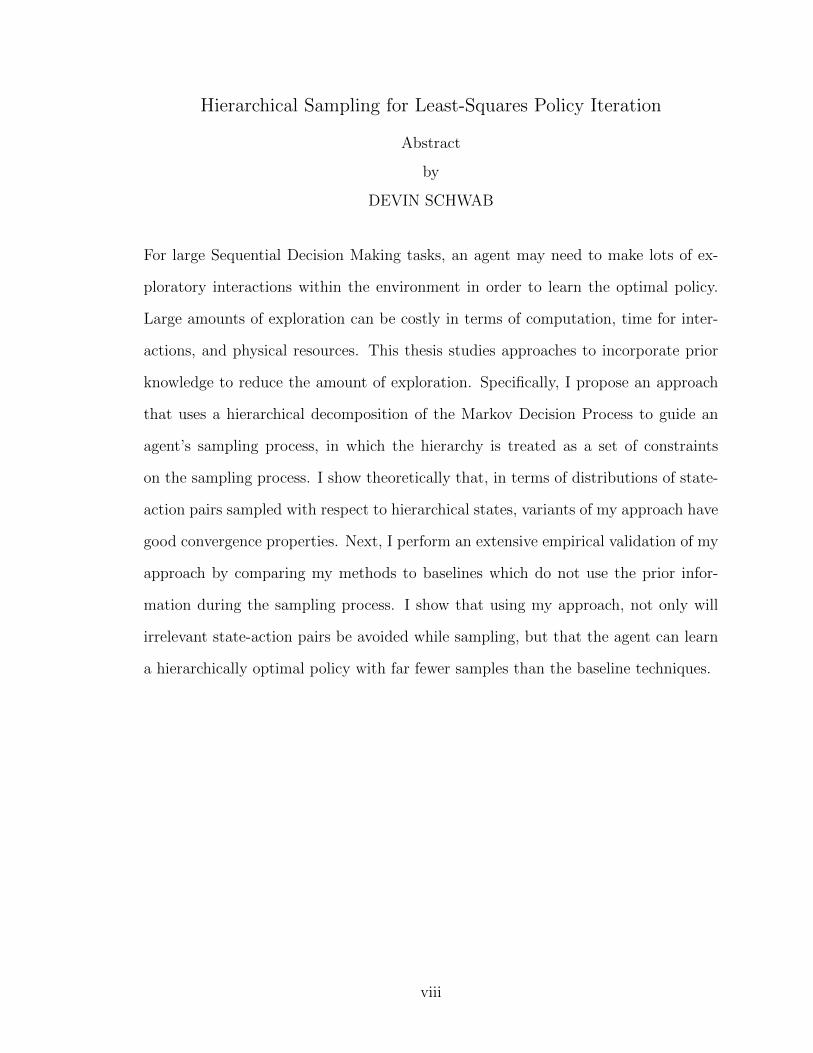
Hierarchical Sampling for Least-Squares Policy Iteration
Abstract
by
DEVIN SCHWAB
For large Sequential Decision Making tasks, an agent may need to make lots of ex-
ploratory interactions within the environment in order to learn the optimal policy.
Large amounts of exploration can be costly in terms of computation, time for inter-
actions, and physical resources. This thesis studies approaches to incorporate prior
knowledge to reduce the amount of exploration. Specifically, I propose an approach
that uses a hierarchical decomposition of the Markov Decision Process to guide an
agent’s sampling process, in which the hierarchy is treated as a set of constraints
on the sampling process. I show theoretically that, in terms of distributions of state-
action pairs sampled with respect to hierarchical states, variants of my approach have
good convergence properties. Next, I perform an extensive empirical validation of my
approach by comparing my methods to baselines which do not use the prior infor-
mation during the sampling process. I show that using my approach, not only will
irrelevant state-action pairs be avoided while sampling, but that the agent can learn
a hierarchically optimal policy with far fewer samples than the baseline techniques.
viii
Chapter 1
Introduction
Every decision has an immediate effect, but more importantly, each decision can also
have long-term consequences. In order to make the best decision, both the immediate
effects and the long-term effects must be taken into account. For instance, choosing
to eat nothing but junk food would be enjoyable in the short term, but the long-
term health consequences are a major problem. Sequential Decision Making (SDM)
is the study of how to make the best decisions when both immediate and long-term
consequences are considered.
Examples of SDM problems abound in the real world. For instance, the everyday
task of what to eat for dinner can be thought of as an SDM. First, what to eat must be
decided, then where to get the ingredients, then how to make it, etc. Each decision
affects the best decisions at the next stage. Algorithms capable of automatically
choosing the optimal actions in these types of situations would be extremely useful
and have wide applicability.
Researchers have been working on designing algorithms that can “solve” an SDM
problem for many years. The simplest and least flexible is to preprogram in the
optimal decision for every scenario. Obviously, this only works for tasks with a very
small amount of scenarios. The other classic approach is to provide the computer, or
1
CHAPTER 1. INTRODUCTION
agent, with a model of how the decisions affect the environment. The agent can then
use this model to plan ahead and choose the best plan of decisions. However, this
approach is not very flexible, as if the environment changes, the model must first be
updated by the programmer.
Rather than providing the agent with lots of information about the SDM, like
planning and preprogramming algorithms, learning algorithms acquire all of their
information about the SDM by interacting with it. Reinforcement Learning (RL)
is the name of the class of algorithms designed to learn how to optimally solve an
SDM from scratch. RL algorithms start out knowing nothing about the environment,
except for the actions it can decide to take. Each time the RL algorithm needs to
make a decision, it examines the environment and consults its policy to determine
what decision to make. In the beginning, the agent has no information about the
effects of decisions, so its policy is random. But as decisions are made, the associated
outcome is tracked. Over time, decisions that had positive outcomes are likely to
be made again, and decisions that had negative outcomes are likely to be avoided.
Eventually, with enough experience the agent will learn a policy that makes the best
decision in every scenario.
For example, consider the task of cooking a meal, which requires the preparation
of a number of different dishes. The agent would need to learn how to boil the
water, cook the pasta, steam the broccoli and plate the food. Each of these different
steps themselves require multiple actions to achieve. An RL agent would start in
the environment knowing nothing about it, except which actions it could decide to
perform. In this case, those actions might be things like “turn on the stove”, “place
the pot on the stove”, “put the pasta in the pot”, “fill the pot with water”, “clean the
broccoli”, “get out the plates”, etc. Because the agent starts with no prior knowledge,
it will randomly try different actions and observe the outcome. In some cases, it will
decide on the right action, like turning on the stove when the pot is already on top.
2
CHAPTER 1. INTRODUCTION
In other cases, it will decide on the wrong action, like putting the pasta in the pot
with no water. In either case, the agent will observe the results of the actions it takes
to learn whether they had positive or negative outcomes. The correct actions, which
have positive outcomes, will then become the actions selected by the agent’s policy.
RL algorithms have many advantages over the planning and preprogramming
approach, however, the example of cooking a meal clearly demonstrates some of the
shortcomings. For example, the agent will waste time trying dumb actions, like
putting an empty pot on the stove. In fact, some of the dumb actions might even be
dangerous. The agent may use the stove incorrectly, thus starting a fire. Therefore,
improvements to the basic RL algorithms that allow for prior information about the
optimal policy are desirable.
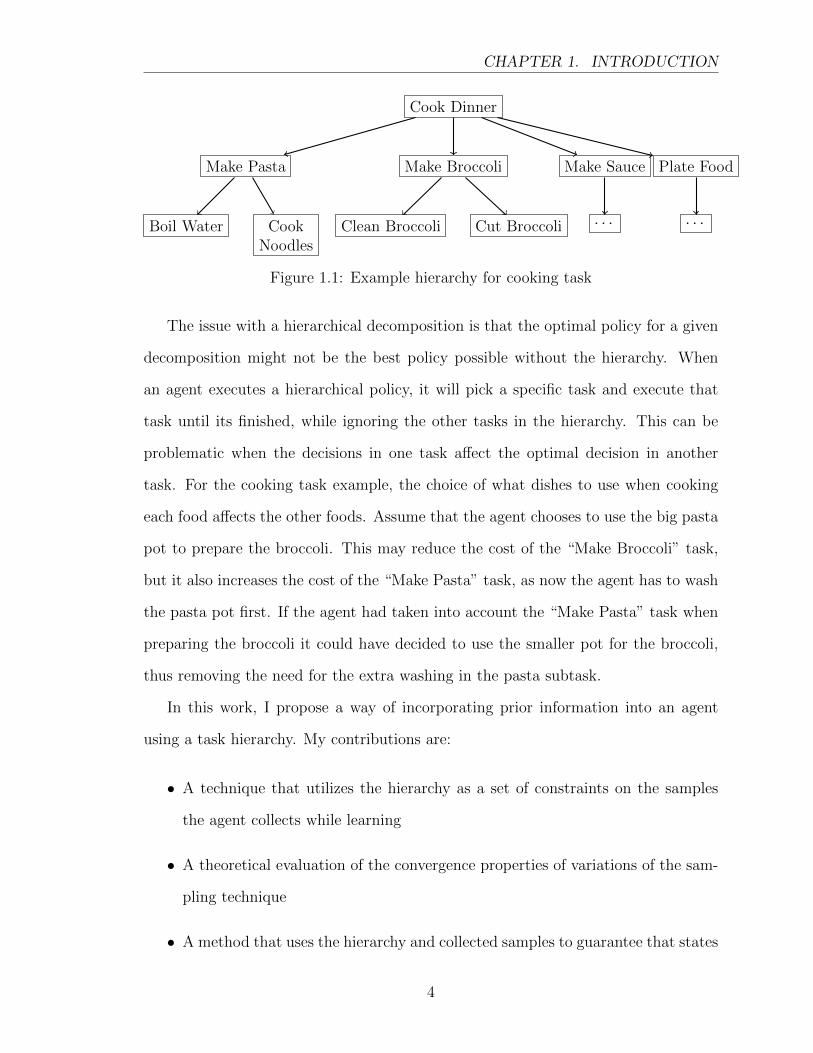
One way to encode prior information is through the use of a hierarchical decom-
position. Rather than trying to solve the whole task at once, the agent can solve
a decomposed version of the task. For example, the meal task can be broken down
by dish: make the pasta, make the broccoli, plate the meal. Each of those tasks
can be further broken down. For instance, the make the broccoli task might contain
the subtasks: clean the broccoli, cut the broccoli, and steam the broccoli. A visual
representation of this is shown in figure 1.1. Now when the agent is trying to learn
how to optimally prepare the broccoli, it will not waste time trying to do things with
the pasta. This can also prevent dangerous actions like turning on the stove when
making the broccoli.
3
CHAPTER 1. INTRODUCTION
Cook Dinner
Make Pasta Make Broccoli Make Sauce Plate Food
Boil Water CookNoodles
Clean Broccoli Cut Broccoli · · · · · ·
Figure 1.1: Example hierarchy for cooking task
The issue with a hierarchical decomposition is that the optimal policy for a given
decomposition might not be the best policy possible without the hierarchy. When
an agent executes a hierarchical policy, it will pick a specific task and execute that
task until its finished, while ignoring the other tasks in the hierarchy. This can be
problematic when the decisions in one task affect the optimal decision in another
task. For the cooking task example, the choice of what dishes to use when cooking
each food affects the other foods. Assume that the agent chooses to use the big pasta
pot to prepare the broccoli. This may reduce the cost of the “Make Broccoli” task,
but it also increases the cost of the “Make Pasta” task, as now the agent has to wash
the pasta pot first. If the agent had taken into account the “Make Pasta” task when
preparing the broccoli it could have decided to use the smaller pot for the broccoli,
thus removing the need for the extra washing in the pasta subtask.
In this work, I propose a way of incorporating prior information into an agent
using a task hierarchy. My contributions are:
• A technique that utilizes the hierarchy as a set of constraints on the samples
the agent collects while learning
• A theoretical evaluation of the convergence properties of variations of the sam-
pling technique
• A method that uses the hierarchy and collected samples to guarantee that states
4
CHAPTER 1. INTRODUCTION
that are inhibited by the hierarchy are inhibited in the policy found by the agent
• A method that uses the hierarchy to generalizes the collected samples in order
to increase the amount of “experience” each sample provides
• Experimental evaluation of my techniques, as compared to baselines, showing
that in many situations my techniques can converge significantly faster than
the baselines
The thesis is organized into three main chapters. In the first chapter, I provide the
necessary background to understand the rest of the thesis. This chapter also includes
references to relevant existing work. The second chapter contains the theoretical
contributions of this thesis. First, I derive the desired distribution of samples for a
task hierarchy. Next, I present the hierarchical sampling algorithm and its variations.
For each variation, I provide a theoretical analysis of the asymptotic properties. I
also introduce the notion of generating samples based on the information in the task
hierarchy. The third chapter contains the hypotheses about the theory along with
their experimental verification. I test each of the sampling variations on a variety
of domains and compare them to existing algorithms as a baseline. I show that my
algorithm can perform significantly better than the baselines over a range of domains.
5
Chapter 2
Background and Related Work
This chapter covers the related background and existing algorithms that are used
in this thesis. First, I define Markov Decision Processs (MDPs), the mathematical
foundation for SDM problems. Then I define the value function, which is a way to
determine the utility of a state and policy. This is followed by an overview of RL algo-
rithms and approximate RL algorithms. Next, I describe Q-learning, a specific online
RL algorithm that is used as a baseline. I then present Least-Squares Policy Iteration
(LSPI), an offline RL algorithm that I use with my hierarchical sampling algorithms.
Next, I present an overview of Hierarchical Reinforcement Learning (HRL). Finally,
I discuss a specific HRL framework, MaxQ, and its associated algorithm.
2.1 Markov Decision Processes (MDP)
The formal way of modeling an SDM process is as an Markov Decision Process (MDP).
MDPs are defined as a tuple (S, S0, A, P,R, γ) [3]. S is the set of all states. These
states are fully observable and contain all of the information the agent needs to
make optimal decisions. S0 ⊆ S is the set of states an agent can start in. It is
possible to have a probability distribution defined over the states in S0, which define
the probability of starting in a particular state from the set. A is the set of actions
6
CHAPTER 2. BACKGROUND AND RELATED WORK
available to the agent. P : S×A×S → [0, 1] is the transition function, a probabilistic
function, which maps state action pairs to resulting states. R : S × A → R is the
reward function, which maps each state action pair to a real value. γ ∈ (0, 1) is the
discount factor, which controls how the agent trades off immediate rewards for long
term rewards. The closer the discount factor is to 1, the more the agent prefers long
term rewards to short term rewards.
As an example, consider a part of the cooking task described in the introduction.
In this case, the set of states, S, contains all of the information about the environment
that the agent needs to know about in order to cook. This might include a binary
variable indicating whether or not the pasta is in the pot, as well as the location of
the agent, the location of the pot and the temperature of the stove. The starting
state would have the stove temperature at room temperature, all of the pots in the
cabinets, and the pasta not in the pot. Some of the actions available might be “put
pasta in pot” and “turn on stove”. The transition function maps actions and states
to resulting states. Let x be a state where the “pasta in pot” variable is false. Let x′
be the state x with the “pasta in pot” variable being true. If the “put pasta in pot”
action has a 90% chance of succeeding in state x, then the transition function would
be P (x, put pasta in pot, x′)→ 0.9 and P (x, put pasta in pot, x)→ 0.1. The reward
function maps states and actions to a real number. If in state x the agent calls the “put
pasta in pot” action, then the reward function might be R(x, put pasta in pot)→ 1.
If there is another state, y, where using action “put pasta in pot” is the wrong action,
then this might have a reward function R(y, put pasta in pot) → −10. Finally, a
reasonable value for γ might be 0.9. The closer γ is to 0, the less the agent will care
about the long term rewards of successfully completing the entire meal task.
At each state, s ∈ S, the agent will choose an action, a ∈ A, using its policy,
π(s) : S → A. The goal of the agent is to learn an optimal policy, which maps each
state in the MDP to the best possible action the agent can make in that state.
7
CHAPTER 2. BACKGROUND AND RELATED WORK
2.1.1 Optimality
The agent’s goal is to learn an optimal policy, π∗, that maximizes the rewards the
agent receives from the MDP. Each execution of a policy gives a specific trajectory,
T , of states the agent entered, and rewards the agent received. The utility of such a
trajectory is shown in equation 2.1.
U(T ) = r0 + γr1 + γ2r2 + · · ·+ γkrk (2.1)
This particular way of calculating a trajectory’s utility is known as cumulative
discounted reward. Other utility functions exist [4], but this work does not deal
with them. Cumulative discounted reward considers all rewards over the course of a
trajectory, but weights short term rewards higher than long term rewards.
While a specific trajectory’s utility can be explicitly calculated, the agent is inter-
ested in finding a policy that generates the trajectory with the best possible utility in
all scenarios. So the agent must select the policy that maximizes over the expected
trajectories according to the policy as seen in equation 2.2. These trajectories may
vary from run to run, based on the starting state, and non-determinism of the actions.
π∗ = argmaxπE [U(T |π)]
= argmaxπE
[∞∑t0
γtrt|π
](2.2)
All algorithms that solve an MDP boil down to trying to solve equation 2.2.
2.2 Value Functions
Learning algorithms solve equation 2.2 by calculating, sometimes indirectly, the value
function over the state space. The value of a state is an estimate of how valuable a
state is to an agent’s policy. Policies that generate trajectories passing through high
8
CHAPTER 2. BACKGROUND AND RELATED WORK
value states are expected to have high utilities as calculated by equation 2.1.
The value function is defined by recursively deconstructing the cumulative dis-
counted reward as shown in equation 2.3. This recursive definition is known as the
Bellman equation [5].
V π(s) = E{rt + γrt+1 + γ2rt+2 + · · · |st = s, π
}= E {rt + γV π(st+1)|st = s, π}
=∑s′
P (s, π(s), s′) (R(s, π(s)) + γV π(s′))
= R(s, π(s)) + γ∑s′∈S
P (s, π(s), s′)V π(s′)
(2.3)
The Bellman equation shows that the value of a state is defined by the value of
the states the agent can transition to, from this state, following the policy π.
The value function allows the agent to compare the quality of two different policies
for a task. A superior policy will have a value function that satisfies the criteria in
equation 2.4.
V π1(s) ≥ V π2(s),∀s ∈ S (2.4)
The goal of the agent is to find a policy π∗, with value function V π∗(s), that
satisfies equation 2.4 when compared to every possible policy’s value function.
2.2.1 Bellman Optimality Equation
To guarantee that a policy is optimal, the agent needs to compare the policy value
function to the optimal value function, V π∗(s). The naıve approach would be to
calculate the value function for every possible policy and then pick whichever policy
satisfied equation 2.4, when compared to all of the other policies. However, there
9
CHAPTER 2. BACKGROUND AND RELATED WORK
are far too many policies to check and the value function can be computationally
expensive to compute for MDPs with large state spaces.
Fortunately, the value of the optimal policy can be computed without knowing the
optimal policy using the Bellman optimality equation shown in equation 2.5. This
equation relates the optimal value of a state, to the optimal value of its neighbors.
Bellman proved that the optimal value function V ∗ = V π∗ under the condition in
equation 2.5.
V ∗(s) = maxa∈A∑s′∈S
P (s, a, s′) (R(s, a) + γV ∗(s′)) (2.5)
The Bellman optimality equation also gives a method of choosing the optimal
action with respect to the value function. Just use the action that gave the best value
in the first place. Equation 2.6 shows this.
π∗(s) = argmaxa∈A∑s′∈S
P (s, a, s′) (R(s, a) + γV ∗(s′)) (2.6)
Bellman Backup Operator
For a given policy, if the model of an MDP is known, then the agent can treat the
Bellman equations as a set of |S| linear equations with |S| unknowns. Each state
must satisfy equation 2.3 and in each state the unknown is V π(s). However, solving
all of the equations simultaneously can be computationally impractical. Instead, an
iterative solution can be defined by transforming the equation into an operator called
the “Bellman Backup Operator”. This is shown in equation 2.7.
(Bπψ)(s) =∑s′∈S
P (s, π(s), s′) (R(s, π(s)) + γψ(s′)) (2.7)
ψ is the set of all real-valued functions over the state space. For a fixed policy, it can
be shown that this backup operator has a fixed point where V π = BπV π. It can also
10
CHAPTER 2. BACKGROUND AND RELATED WORK
be shown that for a fixed policy, Bπ is a monotonic operator, meaning that applying
Bπ to any V 6= V π will always return a V that is closer to V π. That means that for
any initial value function (i.e. V ∈ ψ) repeated application of the backup operator is
guaranteed to converge to the fixed point V π.
Equation 2.7 can also be written in terms of a fixed action a as shown in equa-
tion 2.8.
(Baψ)(s) = R(s, a) + γ∑s′∈S
P (s, a, s′)ψ(s′) (2.8)
Using this formulation, a backup operator that converges on the optimal value
function given any starting value function can be created. The Bellman optimality
criterion showed that the optimal value function is the maximum expected value over
all actions. So, by applying a maximum over all fixed action backups for all states
it is guaranteed that the new value function Vk+1 will be greater than or equal to Vk
for all states. This gives a way to find the optimal value function and therefore, the
optimal policy using the Bellman backup operator. This is shown in equation 2.9.
(B∗ψ)(s) = maxa∈A
(R(s, a) + γ
∑s′∈S
P (s, a, s′)ψ(s′)
)(2.9)
Repeated applications of this will reach the fixed point V ∗ = B∗V ∗.
2.3 Reinforcement Learning
This section presents an overview of RL algorithms. I first define model-free algo-
rithms, which do not require the transition function and reward function of an MDP
in order to find an optimal policy. I compare these to model-based algorithms, which
do require the transition and reward function. Then, I introduce the Quality func-
tion, or Q-function, which is the model-free equivalent to the value function. Next, I
11
CHAPTER 2. BACKGROUND AND RELATED WORK
present the Q-function equivalents of the Bellman equation and Bellman Optimality
equation. Finally, I give an overview of Policy Iteration algorithms.
2.3.1 Model Free Learning
Section 2.2 and 2.2.1 explained how the Bellman equations can be used to find the
Value function of a policy, and from there the optimal policy. The issue is that Value
function based techniques require that the agent have an estimate of the transition
model, P , and reward function, R, of the MDP. Techniques that estimate the model
of the MDP are known as model-based learning algorithms. When a good estimate
of a model can be learned, model-based algorithms perform well, however, often it is
difficult to learn the MDP’s model.
Model-free based algorithms avoid the requirement for a model by instead learning
an estimate of the state-action value function, more commonly called the Quality-
function, or Q-function for short. The Q-function is defined in equation 2.10. Instead
of having single values for every state, each state has as many value as there are
actions. This increases the number of values needed to define the function, but allows
the agent to reason about the value of each specific action in a state individually.
Qπ(s, a) = E{rt + γrt+1 + γ2rt+2 + · · · |st = s, at = a, π
}= E {rt + γQπ(s′, π(s′))|st = s, at = a, π}
=∑s′∈S
P (s, π(s), s′) (R(s, π(s)) + γQπ(s′, π(s′)))
= R(s, a) + γ∑s′∈S
P (s, π(s), s′)Qπ(s′, π(s′))
(2.10)
There is also a form of the Bellman optimality equation for the state-action func-
tion shown in equation 2.11. The main difference between the value function version
is that there is no need to take the maximum with respect to the actions over the
12
CHAPTER 2. BACKGROUND AND RELATED WORK
entire equation. It is only necessary to take the maximum over the inner Q-values.
This saves a large amount of computation and removes the need to reason forward
with the transition function, P .
Q∗(s, a) =∑s′∈S
P (s, a, s′) (R(s, a) + γmaxa′∈AQ∗(s′, a′)) (2.11)
The optimal value function can be obtained using the optimal Q-function by
taking the largest value of the Q-function for each state. This relationship is shown
in equation 2.12.
V ∗(s) = maxa∈AQ∗(s, a) (2.12)
The optimal policy is also easy to find using the optimal Q-function. This is shown
in equation 2.13.
π∗(s) = argmaxa∈AQ∗(s, a) (2.13)
2.3.2 Policy Iteration
An alternative to learning an estimate of the Q-function, is to directly learn the
optimal policy [1]. In reality the exact values of the Q-function do not matter, only
the rankings matter, as the final policy is a maximum over the Q-function. Policy
iteration works directly in policy space and is not concerned with finding the exact
Q-function.
Policy iteration algorithms work in a loop consisting of two steps: policy evalu-
ation and policy improvement. Policy evaluation uses the Bellman backup operator
from equation 2.7 to find the fixed point of the value function for the current policy.
Policy improvement then looks at the value of each state-action pair and determines
if any state-action pairs have better values than the state-action pairs defined by the
13
CHAPTER 2. BACKGROUND AND RELATED WORK
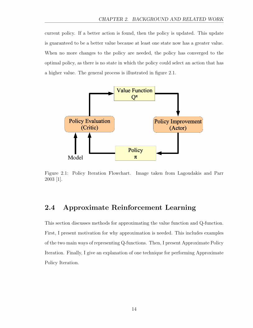
current policy. If a better action is found, then the policy is updated. This update
is guaranteed to be a better value because at least one state now has a greater value.
When no more changes to the policy are needed, the policy has converged to the
optimal policy, as there is no state in which the policy could select an action that has
a higher value. The general process is illustrated in figure 2.1.
Figure 2.1: Policy Iteration Flowchart. Image taken from Lagoudakis and Parr2003 [1].
2.4 Approximate Reinforcement Learning
This section discusses methods for approximating the value function and Q-function.
First, I present motivation for why approximation is needed. This includes examples
of the two main ways of representing Q-functions. Then, I present Approximate Policy
Iteration. Finally, I give an explanation of one technique for performing Approximate
Policy Iteration.
14
CHAPTER 2. BACKGROUND AND RELATED WORK
2.4.1 Value Function Representation
Any RL algorithm that uses the Q-function to solve for the optimal policy, requires
a representation of the Q-function. The most common representation is a table of
values, with one value for each state-action pair. This means that there is no approx-
imation error present in the estimate, however, as the state-action space grows the
number of values needed to represent the Q-function grows. Generally, as the number
of values an agent needs to learn increases, its convergence rate will decrease. In the
most extreme case, the state space is continuous and an exact representation would
require learning an infinite number of values.
Approximation can overcome these issues. The most popular approximation is a
linear combination of features. These features can be as simple as a discretization of
the state space or they can be complex functions hand picked by domain experts. The
only constraint is that the features can only use information from the current state
of the environment and the current set of actions. This is shown in equation 2.14.
Q =n∑i=0
θifi(s, a) (2.14)
Each θ is a weight and fi(s, a) is the i-th feature function. Typically, an extra
feature always equal to 1 is added in to the representation to allow for a constant offset
for the entire linear combination. The weights, θi, are often combined into a single
“weight vector” Θ = [θ0, · · · , θn]. The features are similarly combined into a feature
vector f(s, a) = [f0(s, a), · · · , fn(s, a)]. This allows equation 2.14 to be rewritten in
the more compact form shown in equation 2.15.
Q = Θ · f (2.15)
Now the agent only needs to learn the values of Θ instead of the individual Q-value
of every state-action pair.
15
CHAPTER 2. BACKGROUND AND RELATED WORK
It is important to note that if poor features are chosen, it may be impossible for
the agent to find a reasonable policy. As an extreme example, consider trying to
approximate a policy with a single feature that always evaluates to 1. In this case, all
of the state-action pairs would have exactly the same value, thus making it impossible
for the agent to make intelligent decisions.
The feature representation can also give some generalization to the agent’s expe-
rience. Consider the case where an agent has visited a state s1 many times and has
performed all of the different actions many times. This means that the agent has a
good estimate of the Q-function for that state. Assume that the state has a feature
vector value of fa. If the agent then visits a similar state s2, which has a feature vector
fb, then because s1 is similar to s2 it is likely that fa ≈ fb. This means that the agent
will likely already know the best action in s2 even though it has not visited that state
many times. Features also allow experts in a domain to encode prior knowledge. All
of these upsides can make the feature vector representation a better choice.
2.4.2 Approximate Policy Iteration
Policy iteration using a parametric representation, such as the one shown in equa-
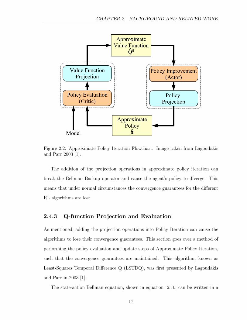
tion 2.15, is known as “Approximate Policy Iteration”. The general process is il-
lustrated in figure 2.2. The process is mostly the same, with the addition of value
function and policy projection operations.
16
CHAPTER 2. BACKGROUND AND RELATED WORK
Figure 2.2: Approximate Policy Iteration Flowchart. Image taken from Lagoudakisand Parr 2003 [1].
The addition of the projection operations in approximate policy iteration can
break the Bellman Backup operator and cause the agent’s policy to diverge. This
means that under normal circumstances the convergence guarantees for the different
RL algorithms are lost.
2.4.3 Q-function Projection and Evaluation
As mentioned, adding the projection operations into Policy Iteration can cause the
algorithms to lose their convergence guarantees. This section goes over a method of
performing the policy evaluation and update steps of Approximate Policy Iteration,
such that the convergence guarantees are maintained. This algorithm, known as
Least-Squares Temporal Difference Q (LSTDQ), was first presented by Lagoudakis
and Parr in 2003 [1].
The state-action Bellman equation, shown in equation 2.10, can be written in a
17
CHAPTER 2. BACKGROUND AND RELATED WORK
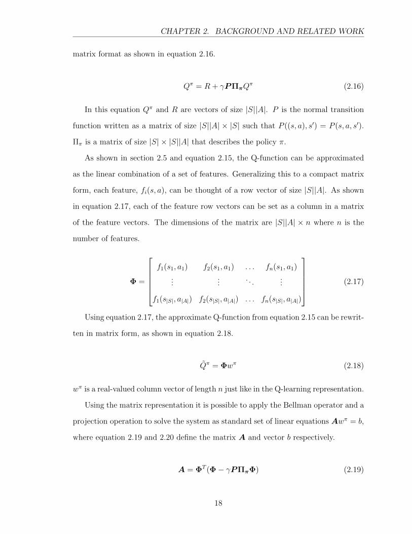
matrix format as shown in equation 2.16.
Qπ = R + γPΠπQπ (2.16)
In this equation Qπ and R are vectors of size |S||A|. P is the normal transition
function written as a matrix of size |S||A| × |S| such that P ((s, a), s′) = P (s, a, s′).
Ππ is a matrix of size |S| × |S||A| that describes the policy π.
As shown in section 2.5 and equation 2.15, the Q-function can be approximated
as the linear combination of a set of features. Generalizing this to a compact matrix
form, each feature, fi(s, a), can be thought of a row vector of size |S||A|. As shown
in equation 2.17, each of the feature row vectors can be set as a column in a matrix
of the feature vectors. The dimensions of the matrix are |S||A| × n where n is the
number of features.
Φ =
f1(s1, a1) f2(s1, a1) . . . fn(s1, a1)
......
. . ....
f1(s|S|, a|A|) f2(s|S|, a|A|) . . . fn(s|S|, a|A|)
(2.17)
Using equation 2.17, the approximate Q-function from equation 2.15 can be rewrit-
ten in matrix form, as shown in equation 2.18.
Qπ = Φwπ (2.18)
wπ is a real-valued column vector of length n just like in the Q-learning representation.
Using the matrix representation it is possible to apply the Bellman operator and a
projection operation to solve the system as standard set of linear equations Awπ = b,
where equation 2.19 and 2.20 define the matrix A and vector b respectively.
A = ΦT (Φ− γPΠπΦ) (2.19)
18
CHAPTER 2. BACKGROUND AND RELATED WORK
b = ΦTR (2.20)
2.5 Q-Learning
Q-learning is one of the most common model-free reinforcement learning algorithms.
Q-learning learns an estimate of the Q-function using feedback from the environment
and then using equation 2.13, the optimal actions for the policy are chosen. The
agent bootstraps itself with a guess for the Q-function, which is refined based on the
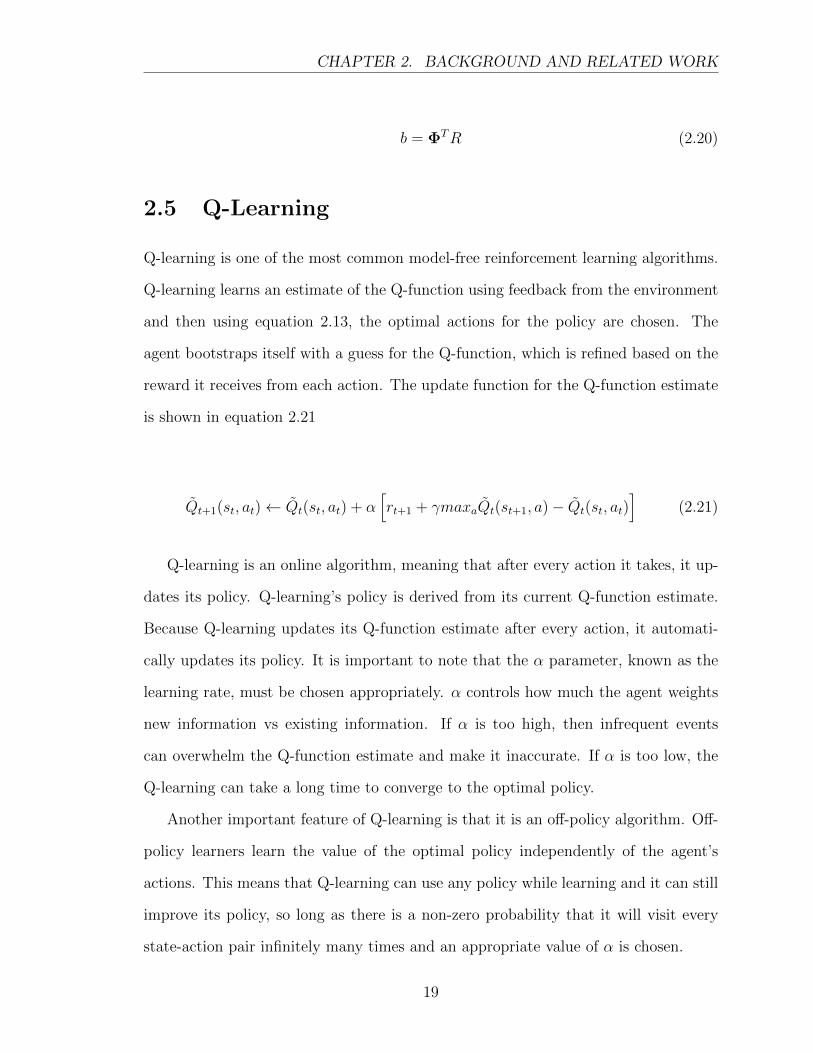
reward it receives from each action. The update function for the Q-function estimate
is shown in equation 2.21
Qt+1(st, at)← Qt(st, at) + α[rt+1 + γmaxaQt(st+1, a)− Qt(st, at)
](2.21)
Q-learning is an online algorithm, meaning that after every action it takes, it up-
dates its policy. Q-learning’s policy is derived from its current Q-function estimate.
Because Q-learning updates its Q-function estimate after every action, it automati-
cally updates its policy. It is important to note that the α parameter, known as the
learning rate, must be chosen appropriately. α controls how much the agent weights
new information vs existing information. If α is too high, then infrequent events
can overwhelm the Q-function estimate and make it inaccurate. If α is too low, the
Q-learning can take a long time to converge to the optimal policy.
Another important feature of Q-learning is that it is an off-policy algorithm. Off-
policy learners learn the value of the optimal policy independently of the agent’s
actions. This means that Q-learning can use any policy while learning and it can still
improve its policy, so long as there is a non-zero probability that it will visit every
state-action pair infinitely many times and an appropriate value of α is chosen.
19
CHAPTER 2. BACKGROUND AND RELATED WORK
2.5.1 Approximate Q-learning
Approximate Q-learning uses the representation from equation 2.15 in conjunction
with the Q-learning update function from equation 2.21 to learn an optimal policy in
an online, off-policy manner. The Q-learning update equation is used with an online
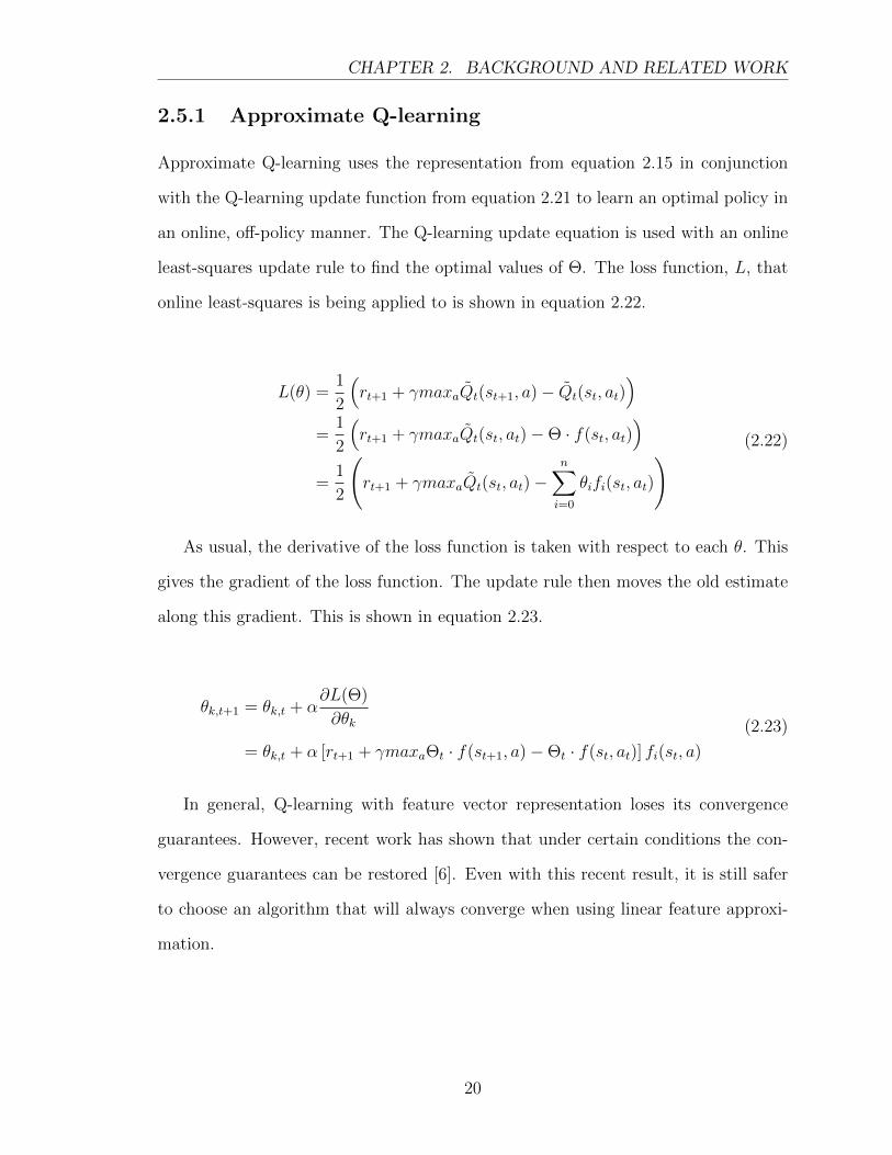
least-squares update rule to find the optimal values of Θ. The loss function, L, that
online least-squares is being applied to is shown in equation 2.22.
L(θ) =1
2
(rt+1 + γmaxaQt(st+1, a)− Qt(st, at)
)=
1
2
(rt+1 + γmaxaQt(st, at)−Θ · f(st, at)
)=
1
2
(rt+1 + γmaxaQt(st, at)−
n∑i=0
θifi(st, at)
) (2.22)
As usual, the derivative of the loss function is taken with respect to each θ. This
gives the gradient of the loss function. The update rule then moves the old estimate
along this gradient. This is shown in equation 2.23.
θk,t+1 = θk,t + α∂L(Θ)
∂θk
= θk,t + α [rt+1 + γmaxaΘt · f(st+1, a)−Θt · f(st, at)] fi(st, a)
(2.23)
In general, Q-learning with feature vector representation loses its convergence
guarantees. However, recent work has shown that under certain conditions the con-
vergence guarantees can be restored [6]. Even with this recent result, it is still safer
to choose an algorithm that will always converge when using linear feature approxi-
mation.
20
CHAPTER 2. BACKGROUND AND RELATED WORK
2.6 Least-Squares Policy Iteration
This section presents the Least-Squares Policy Iteration (LSPI) algorithm. LSPI is
an offline, approximate policy iteration algorithm that represents the policy as a
linear combination of features. First, the policy evaluation and improvement step
of the approximation policy iteration process is described. Then, the overall LSPI
algorithm is shown. The LSPI algorithm provides strong guarantees for convergence
of the policy, even with approximation and projection errors. This makes it a great
choice for large, and complex MDPs that require approximation to efficiently solve.
Least-Squares Temporal Difference Algorithm
Section 2.4.3 explained how the Bellman equations could be constructed in matrix
form and solved as a system of linear equations. Unfortunately the A and b values
cannot be calculated directly by the agent because they require the transition model,
P , and the reward function, R. However, using samples from the environment, A
and b can be estimated. The samples are tuples defined as (s, a, s′, r). s is the state,
in which the agent took action a. r is the reward the agent received for taking the
action a. s′ is the state the agent transitioned to. Algorithm 1 gives the pseudocode
used to iteratively build the estimates of A and b from a set of samples D. This
algorithm is known as Least-Squares Temporal Difference (LSTD) Q as it uses a set
of samples to, in a model free manner, get a least-squares fixed-point approximation
of the Q-function.
21
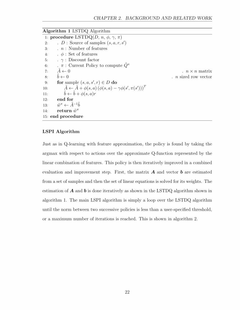
CHAPTER 2. BACKGROUND AND RELATED WORK
Algorithm 1 LSTDQ Algorithm
1: procedure LSTDQ(D, n, φ, γ, π)2: . D : Source of samples (s, a, r, s′)3: . n : Number of features4: . φ : Set of features5: . γ : Discount factor6: . π : Current Policy to compute Qπ
7: A← 0 . n× n matrix8: b← 0 . n sized row vector9: for sample (s, a, s′, r) ∈ D do10: A← A+ φ(s, a) (φ(s, a)− γφ(s′, π(s′)))T
11: b← b+ φ(s, a)r12: end for13: wπ ← A−1b14: return wπ
15: end procedure
LSPI Algorithm
Just as in Q-learning with feature approximation, the policy is found by taking the
argmax with respect to actions over the approximate Q-function represented by the
linear combination of features. This policy is then iteratively improved in a combined
evaluation and improvement step. First, the matrix A and vector b are estimated
from a set of samples and then the set of linear equations is solved for its weights. The
estimation of A and b is done iteratively as shown in the LSTDQ algorithm shown in
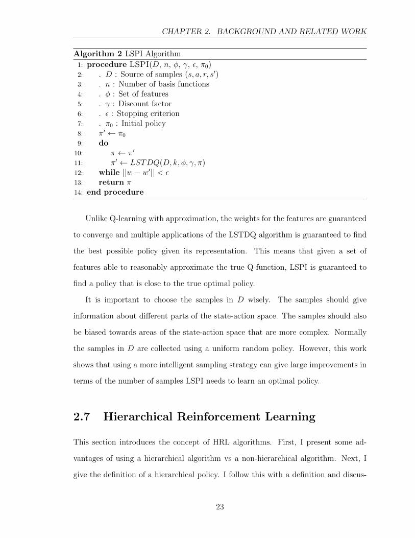
algorithm 1. The main LSPI algorithm is simply a loop over the LSTDQ algorithm
until the norm between two successive policies is less than a user-specified threshold,
or a maximum number of iterations is reached. This is shown in algorithm 2.
22
CHAPTER 2. BACKGROUND AND RELATED WORK
Algorithm 2 LSPI Algorithm
1: procedure LSPI(D, n, φ, γ, ε, π0)2: . D : Source of samples (s, a, r, s′)3: . n : Number of basis functions4: . φ : Set of features5: . γ : Discount factor6: . ε : Stopping criterion7: . π0 : Initial policy8: π′ ← π09: do10: π ← π′
11: π′ ← LSTDQ(D, k, φ, γ, π)12: while ||w − w′|| < ε13: return π14: end procedure
Unlike Q-learning with approximation, the weights for the features are guaranteed
to converge and multiple applications of the LSTDQ algorithm is guaranteed to find
the best possible policy given its representation. This means that given a set of
features able to reasonably approximate the true Q-function, LSPI is guaranteed to
find a policy that is close to the true optimal policy.
It is important to choose the samples in D wisely. The samples should give
information about different parts of the state-action space. The samples should also
be biased towards areas of the state-action space that are more complex. Normally
the samples in D are collected using a uniform random policy. However, this work
shows that using a more intelligent sampling strategy can give large improvements in
terms of the number of samples LSPI needs to learn an optimal policy.
2.7 Hierarchical Reinforcement Learning
This section introduces the concept of HRL algorithms. First, I present some ad-
vantages of using a hierarchical algorithm vs a non-hierarchical algorithm. Next, I
give the definition of a hierarchical policy. I follow this with a definition and discus-
23
CHAPTER 2. BACKGROUND AND RELATED WORK
sion of the two types of optimality possible for a hierarchical policy. I then define
Semi-Markov Decision Processes (SMDPs) and explain what purpose they serve in
the context of the task hierarchy. Finally, I provide a brief overview of some of the
existing HRL frameworks.
2.7.1 Advantages of Hierarchical Reinforcement Learning
Both Q-learning and LSPI are capable, in theory, of solving any MDP optimally,
however, in practice, large MDPs present significant challenges for both algorithms.
The biggest issue is known as “the curse of dimensionality”, which is that the number
of parameters that need to be learned grows exponentially with the size of the state
space. So, as the state-action space grows, the number of samples and the compu-
tational resources needed to find an optimal policy can quickly become intractably
large. Additionally, as the state-action space increases in size the rewards tend to
become sparser, which make the agent’s learning more difficult as it receives less
frequent feedback.
Luckily, many MDPs inherently have structure in terms of their state variables and
reward functions. Inspiration can be taken from human problem solving techniques.
Rather than treating the state-action space as “flat”, an agent can hierarchically
break down the MDP into sub-problems that are much easier to solve.
Breaking a large task into subtasks has many advantages. First, each subtask
will be, by definition, smaller than the full task it was created from. Additionally,
because each subtask is smaller it will take less actions to execute. Therefore, the
reward signals will not need to be propagated as far back along the trajectory of
a policy. Another advantage is that subtasks will often only need to know some of
the state variable values in order to make an optimal decision. This allows each
subtask policy to ignore irrelevant state variables, thus making the subtask MDPs
even smaller.
24
CHAPTER 2. BACKGROUND AND RELATED WORK
In addition to the above advantages, hierarchical MDPs can make it easier to
include prior expert knowledge in an agent. Rather than starting completely from
scratch, an expert can give a hint to the agent in the form of policies for some
of the subtasks and even in the structure of the hierarchy itself. Another way of
including prior information is to use Bayesian priors over the state-action space.
However, previous work has shown that the hierarchical information and the Bayesian
information can complement one another [7]. Essentially, the hierarchy provides
coarse prior information about the overall policy, and Bayesian priors provide fine-
grained prior information at the level of a single state-action pair.
Subtasks also open the possibility to transfer knowledge between agents. Many
MDP hierarchies will have similar subtasks. If a subtask in one MDP already has an
optimal policy it can be used as a starting point for a policy in a similar subtask in
a different MDP.
2.7.2 Hierarchical Policies
In the flat MDP, the agent’s goal is to find a policy that optimizes the expected
rewards the agent will receive. In the hierarchical case, the agent’s goal is to find
a hierarchical policy that optimizes the expected rewards, while conforming to the
hierarchy’s constraints.
A hierarchy is defined by the set of its subtasks, M . Each Mi ∈ M has its own
policy π(i, s). The hierarchical policy is the set of policies for each subtask. The
actions in the subtask policies can be either primitive actions from the original MDP
or subtasks from the hierarchy.
To execute a hierarchical policy, the agent starts in the root task of the hierarchy,
M0. It then consults M0’s policy, π(0, s). π0 gives either a primitive action or a
subtask. If the policy calls for a primitive action, that action is immediately executed.
When the policy calls for a subtask, the agent recurses down into the selected subtask
25
CHAPTER 2. BACKGROUND AND RELATED WORK
and begins executing it according to its policy. The agent continues executing the
chosen subtask until that subtask is finished, at which point it returns to the parent
and continues with the parent policy. This recursive execution of subtask policies
continues until the root task terminates, at which point the original MDP has been
finished.
An alternative execution style is called “polled execution” [2]. Polled execution
makes each decision by starting at the root of the hierarchy. It then recurses down the
hierarchy choosing the child subtask specified by each subtask’s policy. Eventually,
it reaches a primitive action which it executes. It then starts again at the root of the
hierarchy. The main difference is that, in the normal execution style once a subtask
is started it continues executing until it is finished, whereas in polled execution, the
agent starts at the root task every single time.
2.7.3 Hierarchical and Recursive Optimality
The goal of the agent is to find a hierarchical policy that optimizes the expected
rewards it will receive. In all of the hierarchical frameworks the provided hierarchy
constrains the space of possible policies in the underlying MDP. If a good hierarchy
is provided, the agent’s job of learning what to do in the environment is significantly
easier. On the other hand, the restriction in the policy space may prevent the agent
from learning the globally optimal policy. For this reason, hierarchical algorithms
seek a different definition of optimality.
The first type of hierarchical optimality is recursive optimality. In a recursively
optimal policy, each subtask policy is optimal given that its children have optimal
policies. The second type of optimality is hierarchically optimal. In a hierarchically
optimal policy, the policy of a subtask may be suboptimal so that another subtask
can have a better policy. Hierarchically optimal policies are better than recursively
optimal policies, however, to learn a hierarchically optimal policy the subtasks must
26
CHAPTER 2. BACKGROUND AND RELATED WORK
somehow take into account the other subtasks, which complicates the learning pro-
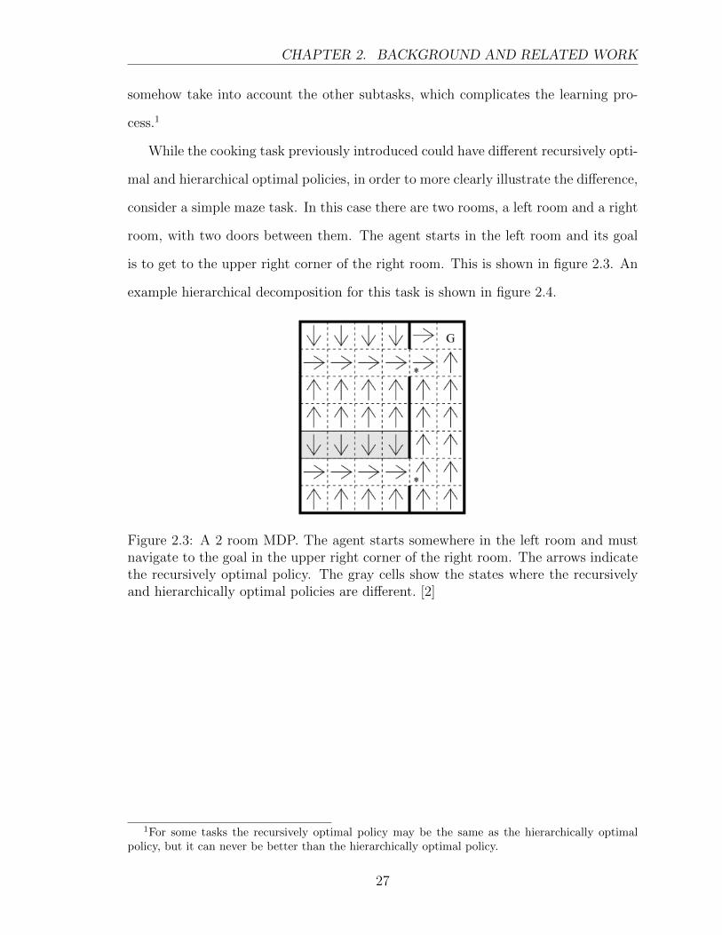
cess.1
While the cooking task previously introduced could have different recursively opti-
mal and hierarchical optimal policies, in order to more clearly illustrate the difference,
consider a simple maze task. In this case there are two rooms, a left room and a right
room, with two doors between them. The agent starts in the left room and its goal
is to get to the upper right corner of the right room. This is shown in figure 2.3. An
example hierarchical decomposition for this task is shown in figure 2.4.
Figure 2.3: A 2 room MDP. The agent starts somewhere in the left room and mustnavigate to the goal in the upper right corner of the right room. The arrows indicatethe recursively optimal policy. The gray cells show the states where the recursivelyand hierarchically optimal policies are different. [2]
1For some tasks the recursively optimal policy may be the same as the hierarchically optimalpolicy, but it can never be better than the hierarchically optimal policy.
27
CHAPTER 2. BACKGROUND AND RELATED WORK
Root
Exit Left Room Navigate Right Room
Navigate(t)
North East South West
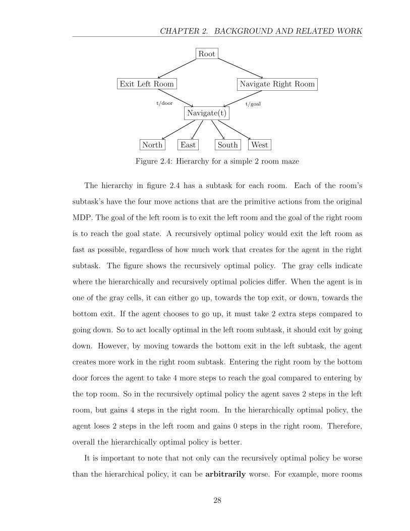
t/door t/goal
Figure 2.4: Hierarchy for a simple 2 room maze
The hierarchy in figure 2.4 has a subtask for each room. Each of the room’s
subtask’s have the four move actions that are the primitive actions from the original
MDP. The goal of the left room is to exit the left room and the goal of the right room
is to reach the goal state. A recursively optimal policy would exit the left room as
fast as possible, regardless of how much work that creates for the agent in the right
subtask. The figure shows the recursively optimal policy. The gray cells indicate
where the hierarchically and recursively optimal policies differ. When the agent is in
one of the gray cells, it can either go up, towards the top exit, or down, towards the
bottom exit. If the agent chooses to go up, it must take 2 extra steps compared to
going down. So to act locally optimal in the left room subtask, it should exit by going
down. However, by moving towards the bottom exit in the left subtask, the agent
creates more work in the right room subtask. Entering the right room by the bottom
door forces the agent to take 4 more steps to reach the goal compared to entering by
the top room. So in the recursively optimal policy the agent saves 2 steps in the left
room, but gains 4 steps in the right room. In the hierarchically optimal policy, the
agent loses 2 steps in the left room and gains 0 steps in the right room. Therefore,
overall the hierarchically optimal policy is better.
It is important to note that not only can the recursively optimal policy be worse
than the hierarchical policy, it can be arbitrarily worse. For example, more rooms
28
CHAPTER 2. BACKGROUND AND RELATED WORK
can be added in order to make the two-rooms domain recursively optimal policy worse
than it is consider that in the two-rooms domain to make the recursively optimal
policy worse than it. Each room can have the sub-optimality shown in the example
present. So, by adding in more rooms between the agent and the goal it is possible
to construct an example of a domain where the recursively optimal policy will be
arbitrarily worse than the hierarchically optimal policy.
2.7.4 Semi-Markov Decision Processes
One complication that arises from a hierarchical decomposition of a regular MDP,
is that the subtasks become Semi-Markov Decision Processes (SMDPs). The main
difference between an SMDP and an MDP is that an SMDP has actions that take
multiple time steps. While this distinction does not add any new representational
capabilities compared to a standard MDP, it does make specifying the problem much
easier. While an action is executing, the state may change multiple times and the
agent may receive multiple reward signals.
Just like an MDP, an SMDP is defined as a tuple (S, S0, A, P,R, γ). S, S0, and
A are all defined the same as a regular MDP, only P and R differ. In an MDP the
transition function was defined as the P (s, a, s′) or the probability of starting in state
s, executing action a and ending in state s′. In an SMDP the actions can take multiple
time steps so the function requires another input parameter N . P (s, a,N, s′) is the
probability of starting in state s, taking durative action a and this action then taking
N steps and ending with the agent in state s′. As mentioned, an SMDP adds no
extra representational power because if the transition model is marginalized over the
variable N a normal MDP transition model is obtained for the underlying MDP. The
reward function is similarly changed to include a number of time steps from action
a until a reward is received. That is R(s, a,N) is the function R : S × A ×N → R,
which defines the reward received N time steps into the execution of action a from
29
CHAPTER 2. BACKGROUND AND RELATED WORK
state s. Just as P can be marginalized over N to receive the underlying MDPs
transition model, R can be marginalized over N to receive the underlying MDPs
reward function. The γ term remains the same as in the original MDP tuple.
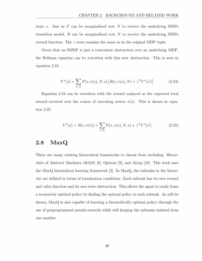
Given that an SMDP is just a convenient abstraction over an underlying MDP,
the Bellman equation can be rewritten with this new abstraction. This is seen in
equation 2.24.
V π(s) =∑s′,N
P (s, π(s), N, s)[R(s, π(s), N) + γNV π(s′)
](2.24)
Equation 2.24 can be rewritten with the reward replaced as the expected total
reward received over the course of executing action π(s). This is shown in equa-
tion 2.25.
V π(s) = R(s, π(s)) +∑s′,N
P (s, π(s), N, s) + γNV π(s′) (2.25)
2.8 MaxQ
There are many existing hierarchical frameworks to choose from including: Hierar-
chies of Abstract Machines (HAM) [8], Options [9], and ALisp [10]. This work uses
the MaxQ hierarchical learning framework [2]. In MaxQ, the subtasks in the hierar-
chy are defined in terms of termination conditions. Each subtask has its own reward
and value function and its own state abstraction. This allows the agent to easily learn
a recursively optimal policy by finding the optimal policy in each subtask. As will be
shown, MaxQ is also capable of learning a hierarchically optimal policy through the
use of preprogrammed pseudo-rewards while still keeping the subtasks isolated from
one another.
30
CHAPTER 2. BACKGROUND AND RELATED WORK
2.8.1 MaxQ Hierarchy
MaxQ takes the MDP, M , and divides it into a hierarchy of n subtasks, (M0, · · · ,Mn).
Each of the tasks shown in the hierarchy is specified by a three tuple, (Ti, Ai, Ri).
Ti(si) is a logical predicate that partitions the states in S into a set of active states Si
and terminal states Ti. The agent can only execute subtask Mi when the current state
s is in Si. Ai is the set of actions that can be performed in subtask Mi. This can be a
primitive action from the original MDP’s set A or a subtask from the hierarchy. If a
child subtask Mj has parameters then it will appear in Ai once for each of the possible
bindings. Ri(s, a) is a pseudo-reward function which specifies expert coded rewards
when the agent transitions from a state s ∈ Si to a state s′ ∈ Ti. This function
gives the agent an idea of how desirable a specific termination state is, which can
allow MaxQ to find hierarchically optimal policies while treating each subtask as
independent.
MaxQ executes the policy using a stack and each subtask’s policy. The agent
starts with an empty execution stack. It then checks the root subtask’s policy to
determine which action to call. If the action is a primitive action, the agent executes
it and then walks back up the execution stack until a non-terminal subtask is reached.
If the action is a non-primitive action, then it recurses down the hierarchy selecting
the best action from each subtask’s policy until a primitive action is reached.
While each subtask has its own policy, the value of the policy is determined by
the value of its children subtasks and primitive actions. The next section explains
how the value function is hierarchically decomposed.
2.8.2 Value Function Decomposition
Recall that the value function is expectation over the cumulative discounted rewards
the agent will receive while executing a policy π. The difference in MaxQ is that now
there is a value function for every subtask. So, the value function is parameterized
31
CHAPTER 2. BACKGROUND AND RELATED WORK
by the subtask index as shown in equation 2.26.
V π(i, s) = E{rt + γrt+1 + γ2rt+2 + · · · |st = s, π
}(2.26)
Consider if the policy πi chooses the subroutine a. Subroutine a will run for
a number of steps, N , and then terminate in state s′ according to the transition
model for the subtask i, P πi (s, a,N, s′). This means that the value function from
equation 2.26 can be split into the expectation over two summations as shown in
equation 2.27.
V π(i, s) = E
{N−1∑k=0
γkrt+k +∞∑k=N
γkrt+k|st = s, π
}(2.27)
The first summation is the discounted sum of rewards obtained while executing
the subtask a from state s to termination. In other words V π(a, s) =∑N−1
k=0 γkrt+k.
The second term is the value of continuing the policy from state s′, V π(i, s′), with a
discount equal to the number of steps it took a to terminate. Equation 2.27 can be
rewritten as equation 2.28. This equation is of the same form as the standard MDP
Bellman equation shown in equation 2.25. In this case R(s, π(s)) = V π(πi(s), s).
V π(i, s) = V π(πi(s), s) +∑s′,N
P πi (s, πi(s), N, s
′)γNV π(i, s′) (2.28)
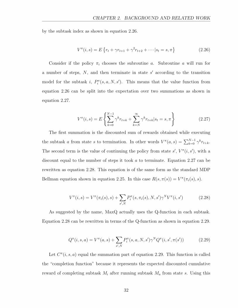
As suggested by the name, MaxQ actually uses the Q-function in each subtask.
Equation 2.28 can be rewritten in terms of the Q-function as shown in equation 2.29.
Qπ(i, s, a) = V π(a, s) +∑s′,N
P πi (s, a,N, s′)γNQπ(i, s′, π(s′)) (2.29)
Let Cπ(i, s, a) equal the summation part of equation 2.29. This function is called
the “completion function” because it represents the expected discounted cumulative
reward of completing subtask Mi after running subtask Ma from state s. Using this
32
CHAPTER 2. BACKGROUND AND RELATED WORK
new definition, equation 2.29 can be rewritten recursively as in equation 2.30.
Qπ(i, s, a) = V π(a, s) + Cπ(i, s, a) (2.30)
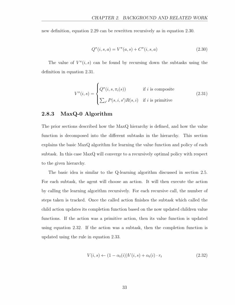
The value of V π(i, s) can be found by recursing down the subtasks using the
definition in equation 2.31.
V π(i, s) =
Qπ(i, s, πi(s)) if i is composite∑
s′ P (s, i, s′)R(s, i) if i is primitive
(2.31)
2.8.3 MaxQ-0 Algorithm
The prior sections described how the MaxQ hierarchy is defined, and how the value
function is decomposed into the different subtasks in the hierarchy. This section
explains the basic MaxQ algorithm for learning the value function and policy of each
subtask. In this case MaxQ will converge to a recursively optimal policy with respect
to the given hierarchy.
The basic idea is similar to the Q-learning algorithm discussed in section 2.5.
For each subtask, the agent will choose an action. It will then execute the action
by calling the learning algorithm recursively. For each recursive call, the number of
steps taken is tracked. Once the called action finishes the subtask which called the
child action updates its completion function based on the now updated children value
functions. If the action was a primitive action, then its value function is updated
using equation 2.32. If the action was a subtask, then the completion function is
updated using the rule in equation 2.33.
V (i, s)← (1− αt(i))V (i, s) + αt(i) · rt (2.32)
33
CHAPTER 2. BACKGROUND AND RELATED WORK
C(i, s, a)← (1− αt(i)) · C(i, s, a) + αt(i) · γNV (i, s′) (2.33)
Throughout both of the algorithms the value function is needed. Equation 2.34
shows how these numbers are defined. Evaluating these values requires a complete
search of all paths through the MaxQ hierarchy staring at node i and ending at all
of the leaf nodes that are descendants of i.
V (i, s) =
maxaQ(i, s, a) if i is composite
V (i, s) if i is primitive
Q(i, s, a) = V (a, s) + C(i, s, a)
(2.34)
Just like Q-learning, the MaxQ paper proves that so long as each state-action pair
in a subtask has a non-zero probability of being visited an infinite number of times,
then MaxQ is guaranteed to converge.
2.8.4 Pseudo-Rewards
The issue with the MaxQ-0 algorithm is that each subtask’s policy is computed op-
timally with respect to its children. This is the definition of recursive optimality.
However, as shown, a better type of optimality, hierarchical optimality, exists. The
issue with finding hierarchically optimal policy is that the subtasks can no longer be
treated as independent. Now the execution stack for a policy effects which terminal
state a subtask should try to end in. This was shown in the two rooms example.
MaxQ deals with the suboptimality of a recursively optimal policy by allowing
each subtask to define a pseudo-reward function, Ri. Pseudo-rewards are hand-coded,
fixed reward functions included in the MaxQ hierarchy definition. The pseudo-reward
function can only be non-zero for state-action pairs that transition to a termination
state for the subtask. These extra rewards are included in addition to the true MDP
34
CHAPTER 2. BACKGROUND AND RELATED WORK
rewards received by the agent during execution. The purpose of the pseudo-reward
is to allow the programmer to weight a particular subtask exit up or down according
to how useful that exit is in the next subtask to be executed.
To illustrate how this works, consider the previous two rooms example from sec-
tion 2.7.3. In this domain the recursively optimal policy moves the agent to the
closest door, but the hierarchically optimal policy moves the agent to the top door.
As was shown, the hierarchically optimal policy has a greater value than the recur-
sively optimal policy, even though the hierarchical policy’s left room subtask has a
locally suboptimal policy.
If MaxQ-0 was run on the two rooms domain, it would converge to the recursively
optimal policy because MaxQ-0 does not use pseudo-rewards. However, if a pseudo-
reward function is defined for the left room subtask, the programmer can give a
pseudo-reward of +10 to the top exit. The left subtask can use this pseudo reward
when calculating its internal policy. This will cause the left room policy to always
use the top door, thus making the whole policy hierarchically optimal.
MaxQ-0 can be modified into the MaxQ algorithm by tracking two completion
functions for each subtask. One completion function, which uses the pseudo-rewards,
determines the internal policy of that subtask. The other completion function is the
same as the one used in MaxQ-0. This completion function is used by the parent
subtask when computing the values of its actions. Separate completion functions are
needed to guarantee that the pseudo-rewards of a task do not “contaminate” the
other SMDPs, which would change the MDP that was being solved.
35
Chapter 3
Hierarchical Sampling
This chapter explains the contributions of this work and provides a theoretical anal-
ysis of the contributions. First, I give motivation for why hierarchical sampling is
needed. Then, I present my hierarchical sampling algorithm. To prove the theoreti-
cal properties of variations of this algorithm I define an operation, called “Hierarchical
Projection”, which maps the distribution of samples in the hierarchical MDP to the
distribution of samples in the flat MDP. Next, I present three variations of the hierar-
chical sampling algorithm and prove asymptotic convergence properties with respect
to the target distribution. Following the hierarchical sampling algorithm explanation,
I introduce the concept of “derived samples”, which are samples generated from the
hierarchy. I first present inhibited action samples, which teach the flat policy solver
which actions are inhibited by the hierarchy. I then present abstract samples which
generalize samples across multiple states using information in the hierarchy about ir-
relevant state variables. Finally, I show the full algorithm using hierarchical sampling,
hierarchy samples and LSPI.
36
CHAPTER 3. HIERARCHICAL SAMPLING
3.1 Motivation
As discussed in section 2.7.1, hierarchical algorithms have many advantages over
traditional flat algorithms. Even so, HRL algorithms often settle for a recursively
optimal policy. By sacrificing global and hierarchical optimality the space of possible
possibles is greatly restricted. This can lead to huge increases in the rate of conver-
gence to the optimal policy. Also, computing a recursively optimal policy is generally
much easier, as when computing a hierarchically optimal policy all of the subtask
interactions must be considered. The issue with recursively optimal policies is that,
as shown in section 2.7.3, recursively optimal policies can be arbitrarily worse than
the hierarchical optimal policy. So even though HRL algorithms, which guarantees
recursive optimality, can greatly speed up the convergence of the policy, the policy it
converges to might not be any good!
MaxQ attempts to solve this trade-off between computational complexity and
the optimality of the policy through pseudo-rewards, however, pseudo-rewards have
their own issues. If the proper pseudo-rewards are set for the tasks in the hierarchy
then MaxQ can find the hierarchically optimal policy with very little extra overhead.
However, picking the proper pseudo-rewards can be difficult in practice. In general
the expert needs to have an idea of what the optimal policy looks like in order to pick
good values. Also, if poor values are chosen, then the pseudo-rewards can do more
harm than good. For instance, consider if the incorrect pseudo-rewards are chosen
for the two rooms domain from section 2.7.3. If a positive pseudo-reward is placed on
the top door then MaxQ will converge to the hierarchically optimal policy. However,
if instead a positive pseudo-reward is placed on the bottom door MaxQ will actually
do worse than the recursively optimal policy, as now the agent will always try to exit
through the bottom door.
Despite these shortcomings, HRL algorithms still have a number of advantages
over flat RL algorithms. Q-learning, LSPI and other flat RL algorithms can take
37
CHAPTER 3. HIERARCHICAL SAMPLING
a long time to learn when the state-action space of an MDP is large. The “curse
of dimensionality” can be a major issue for many algorithms. As the state space
grows, the computational resources can increase exponentially with the size of the
state space. Additionally, as the state-action space becomes larger the reward signals
tend to be sparser. This means the agent will have to wait longer before it receives
feedback. When feedback is received a long time after the action takes place, it can
be difficult for the agent to determine what the exact cause of the feedback was, thus
making it difficult to determine the optimal actions for a policy.
Another downside of flat algorithms is that they can lack an easy way to encode
prior information. Bootstrapping the agent with prior information can help the agent
converge to the optimal policy faster by more accurately directing the exploration
and policy search. Without prior information, the agent’s initial policy is random,
which puts the agent at a high risk of doing something dangerous to its environment
or itself. For simulated domains this is not a concern, but for an agent in the real
world, such as a robot, this might be a major concern.
Previous work has shown that Bayesian priors can encode some prior information
about particular state-action pairs. However, it has been shown that this information
is actually different than the type of information that a hierarchical decomposition
gives [7]. It is possible to include Bayesian priors on possible policies, however, this
has its own issues. In general, it is difficult to compute with policy priors. Also, policy
priors do not allow for state and action abstraction like a task hierarchy. Therefore,
even if Bayesian priors are used there is still a use for the task hierarchy information.
Hierarchies also break the large MDP down into smaller, easier to solve subtasks.
This allows the agent to abstract away state variables and actions that are irrelevant
in each sub problem, making each subtask easier to solve. This type of decomposi-
tion also encodes relationships between the subtasks based on their positions in the
hierarchy. Related tasks will be in the same subgraph, and unrelated subtasks will
38
CHAPTER 3. HIERARCHICAL SAMPLING
not. Consider the kitchen example discussed previously. If the agent wants to cook
the pasta then it does not need to concern itself with the actions related to cooking
the broccoli. Additionally it does not need to concern itself with the parts of the
state that are related to the broccoli when cooking the pasta, as they have no effect
on the task at hand.
One of the major advantages of MaxQ is the ability for state abstraction. Even
though the decomposition creates more SMDPs to be solved, these SMDPs can elimi-
nate irrelevant state variables. This makes the state-action space of each SMDP much
smaller and thus easier to solve. However, even with state abstraction it is still pos-
sible to have too large of a state space. For example, if a state variable is continuous,
it is impossible to use the tabular representation that MaxQ uses in each subtask. In
theory it is possible to use a feature based representation like in Q-learning or LSPI,
but just like in Q-learning, the convergence guarantees are lost.
Ideally, an algorithm could be created that has the advantages of the flat methods
(better than recursively optimal policies and feature approximation) with the advan-
tages of the hierarchical algorithms (faster convergence, state abstraction, elimination
of irrelevant actions while learning). This thesis presents an algorithmic framework
that accomplishes these things.
3.2 Hierarchical Sampling Algorithm
The main contribution of this work is a method of using a task hierarchy as a set
of constraints on the sampling process. A normal, offline, “flat” RL algorithm can
then use these samples to converge to a policy both faster and safer. The sampling
technique is separated from the actual learning, meaning that in theory it can be
used with any offline learning algorithm, however, this work focuses on applying it
with the LSPI algorithm. This work focuses on using a MaxQ hierarchy to construct
39
CHAPTER 3. HIERARCHICAL SAMPLING
the constraints, but in theory any hierarchical framework could be used in a similar
manner.
At each state the hierarchy has terminated subtasks and non-terminated subtasks.
The terminated subtasks form constraints on the actions that can be taken. If an
action is unavailable in every executable subtask, then the hierarchy constrains the
agent so that it will not try that action. This makes sure that the agent spends its
time exploring actions that are actually relevant to the state. The hierarchy can also
be defined to disallow dangerous actions in certain states. In that case this sampling
technique will also stop the agent from executing the dangerous actions.
The second part of the contributions uses the collected samples and the hierarchy
to derive new samples. These samples are referred to as “derived samples”. There are
two types of derived samples: inhibited action samples and abstract samples. Inhib-
ited action samples are generated for actions the agent was disallowed from testing,
due to the hierarchy constraints. These samples guarantee that the policy found by
the agent never chooses these actions. The second type of sample, abstract samples,
generalize individual samples across irrelevant state variables. The information in the
original sample is duplicated and irrelevant state variables are varied to indicate to
the agent, that no matter the value of the irrelevant state variables, the action will
have the same outcome.
The sampling collection algorithm dictates how the agent goes about collecting
the “real” samples. Whereas in normal sampling a uniform random policy over the
state-action space is used, the sampling strategies presented in this work modify
this probability distribution via the hierarchy. This thesis presents three different
variations on this technique.
40
CHAPTER 3. HIERARCHICAL SAMPLING
3.3 Sampling Algorithm
The standard way for an agent to select actions when collecting samples from an
MDP, is to use a uniform random policy. In every state, the agent selects with
uniform random probability an available action. So if three actions are available, the
chance that the agent will try any of one of them is one-third. This type of sampling
policy has the advantage that as the number of samples it collects approaches infinity,
the probability that it has seen every state-action pair goes to 1. This ensures that
eventually the agent will have enough information to find the optimal policy.
The issue with a uniform random policy, is that many actions are only relevant in
a small subset of the state space. This means that the agent will waste a lot of samples
trying actions that will never be relevant. If the agent knew ahead of time how likely
an action is to be relevant in a given state, it could bias its sample collection towards
these actions.
The kitchen domain provides a good example of a case where some actions are
irrelevant in most of the state space. In the kitchen task many of the actions require
very specific states. For instance, placing the pasta in the water should only be done
after the water is boiled. Also, plating the food should only be done after the food is
cooked. The MaxQ agent, by virtue of the hierarchy, knows that putting the pasta
in the water is unlikely to be the correct action. It also knows that until the food is
ready, the plating actions are completely irrelevant.
An even more pressing issue with a uniform random policy is that the agent may
select actions that are dangerous to itself or the environment. These actions may
prevent the agent from ever completing its task. For instance, turning on the stove is
essential to cooking the meal, however, if the stove is turned on at an inappropriate
time the agent may get burned or start a fire. Even if an action doesn’t cause physical
harm, it may transition the agent to a state in which it can never complete its task. If
the agent does an incorrect action when preparing the food, it may ruin the ingredients
41
CHAPTER 3. HIERARCHICAL SAMPLING
and be unable to ever finish preparing the meal.
The MaxQ agent can avoid ruining the ingredients by limiting the actions that can
be applied to subtasks via termination conditions. Whenever the agent is in a state
where it is not safe to do an action, then the subtasks containing that action should
be in a terminated state. This will prevent MaxQ from ever using the dangerous
actions.
The most basic contribution of this work is the design and analysis of a sampling
algorithm that directs how the agent collects its real samples so that dangerous state-
action pairs are avoided. The distribution of actions in each state is also biased to
select actions that, according to the hierarchy, are more likely to be relevant. The
algorithm uses the same hierarchy provided by the MaxQ framework. Three specific
variations on this basic algorithm are presented and analyzed. They are referred to as:
Random Hierarchical Policy (RHP) sampling, Weakly Polled sampling, and Polled
sampling. A theoretical analysis of the different properties of the variations is also
presented.
3.3.1 Hierarchical Projection
When the agent is executing a hierarchical policy, the state space no longer consists of
just the state of the environment, S. It now consists of the callstack used to reach the
current subtask, Mi. The callstack can be thought of as a path through the hierarchy
from the root task to the current subtask which is being executed. For example,
in the kitchen task hierarchy, shown in figure 1.1, if the agent is executing “cook
noodles” subtask, then the callstack would be “{cook dinner, make pasta}”. The
hierarchies are actually poly-trees meaning that some subtasks may have multiple
possible callstacks. For example, in the two-rooms hierarchy, shown in figure 2.4,
the navigate subtask is a child of both “Exit left root” and “Navigate right room”.
This means that when executing navigate there are two callstacks possible “{Root,
42
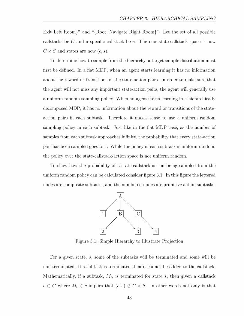
CHAPTER 3. HIERARCHICAL SAMPLING
Exit Left Room}” and “{Root, Navigate Right Room}”. Let the set of all possible
callstacks be C and a specific callstack be c. The new state-callstack space is now
C × S and states are now (c, s).
To determine how to sample from the hierarchy, a target sample distribution must
first be defined. In a flat MDP, when an agent starts learning it has no information
about the reward or transitions of the state-action pairs. In order to make sure that
the agent will not miss any important state-action pairs, the agent will generally use
a uniform random sampling policy. When an agent starts learning in a hierarchically
decomposed MDP, it has no information about the reward or transitions of the state-
action pairs in each subtask. Therefore it makes sense to use a uniform random
sampling policy in each subtask. Just like in the flat MDP case, as the number of
samples from each subtask approaches infinity, the probability that every state-action
pair has been sampled goes to 1. While the policy in each subtask is uniform random,
the policy over the state-callstack-action space is not uniform random.
To show how the probability of a state-callstack-action being sampled from the
uniform random policy can be calculated consider figure 3.1. In this figure the lettered
nodes are composite subtasks, and the numbered nodes are primitive action subtasks.
A
B C1
2 3 4
Figure 3.1: Simple Hierarchy to Illustrate Projection
For a given state, s, some of the subtasks will be terminated and some will be
non-terminated. If a subtask is terminated then it cannot be added to the callstack.
Mathematically, if a subtask, Mi, is terminated for state s, then given a callstack
c ∈ C where Mi ∈ c implies that (c, s) 6∈ C × S. In other words not only is that
43
CHAPTER 3. HIERARCHICAL SAMPLING
subtask impossible to enter, its children cannot be entered.
The callstack of a subtask is essentially a path through the hierarchy. There-
fore, for a given state, the probability of a specific callstack being sampled is the
probability of traversing the hierarchy via that callstack’s path. The probability of
traversing a specific path is the probability of each of the path’s segments being cho-
sen. Each segment in the path is determined by the selected child subtask and the
children subtasks are selected via a uniform random sampling policy in each subtask.
Equation 3.1 shows the probability of selecting a specific path segment.
P (Mi|s) =1
#children(Mi|s)(3.1)
In this equation Mi is the current subtask being sampled. #children(Mi|s) is the
number of non-terminated children of subtask Mi for the state s. The probability is
conditioned on the state s because the set of non-terminated subtasks depends on the
current state.
The segments are all chosen independently of one another, so to get the full path
probability, all of the individual segment probabilities are multiplied. Equation 3.2
shows the probability for a path in the hierarchy. In this equation the S variables
represent segments in the path.
P (c|s) = P ((S0, S1, · · · , Sn)|s)
= P (S0|s)P (S1|s) · · ·P (Sn|s)
=1
#children(M0|s)#children(M1|s) · · ·#children(Mn|s)
(3.2)
For example, consider a state s where all of the subtasks in the hierarchy from
figure 3.1 are non-terminated. In this case the probability of the callstack “{A, B,
3}” being chosen in state s, will be P (((A,B), (B, 3))|s) = 16. Using equation 3.1,
the probability of segment (A,B) being chosen is P ((A, b)|s) = 13
and the prob-
44
CHAPTER 3. HIERARCHICAL SAMPLING
ability of segment (B, 3) being chosen is P ((B, 3)|s) = 12. These values can be
used with equation 3.2 to get the final probability of the full path. In this case
P (((A,B), (B, 3))|s) = P ((A,B)|s)P ((B, 3)|s) = 16.
Equations 3.1 and 3.2 define the target distribution over the state-callstack space.
However, my sampling algorithms use the hierarchy to collect samples in the original
flat state-action space. Therefore it is necessary to define the “hierarchy projection”
operation which maps the state-callstack distribution to a state-action distribution.
The flat samples only keep information about which primitive actions were tried
in what state, they do not contain information about the callstack at the time the
action was sampled. Therefore, to project the hierarchical distribution down to a flat
distribution for each state-action pair in the flat MDP, the probability is the sum
of all of the state-callstacks which have that action at the top. This is shown in
equation 3.3.
P (a|s) =∑
∀c∈C,a∈c
P (c|s) (3.3)
As a sanity check, consider a flat MDP with no prior information known. This flat
MDP can be transformed into a hierarchy with a single root task and every primitive
action as a child of the root task. Figure 3.2 shows an example of what this might
look like. This hierarchy tells the agent that all tasks are relevant to the root task and
that all are equally likely to be relevant. Essentially it contains no information that
the flat MDP does not have. Therefore, we would expect the projected hierarchical
distribution to be uniform over the state-action space. Using the equation 3.3 this
indeed is the case.
45
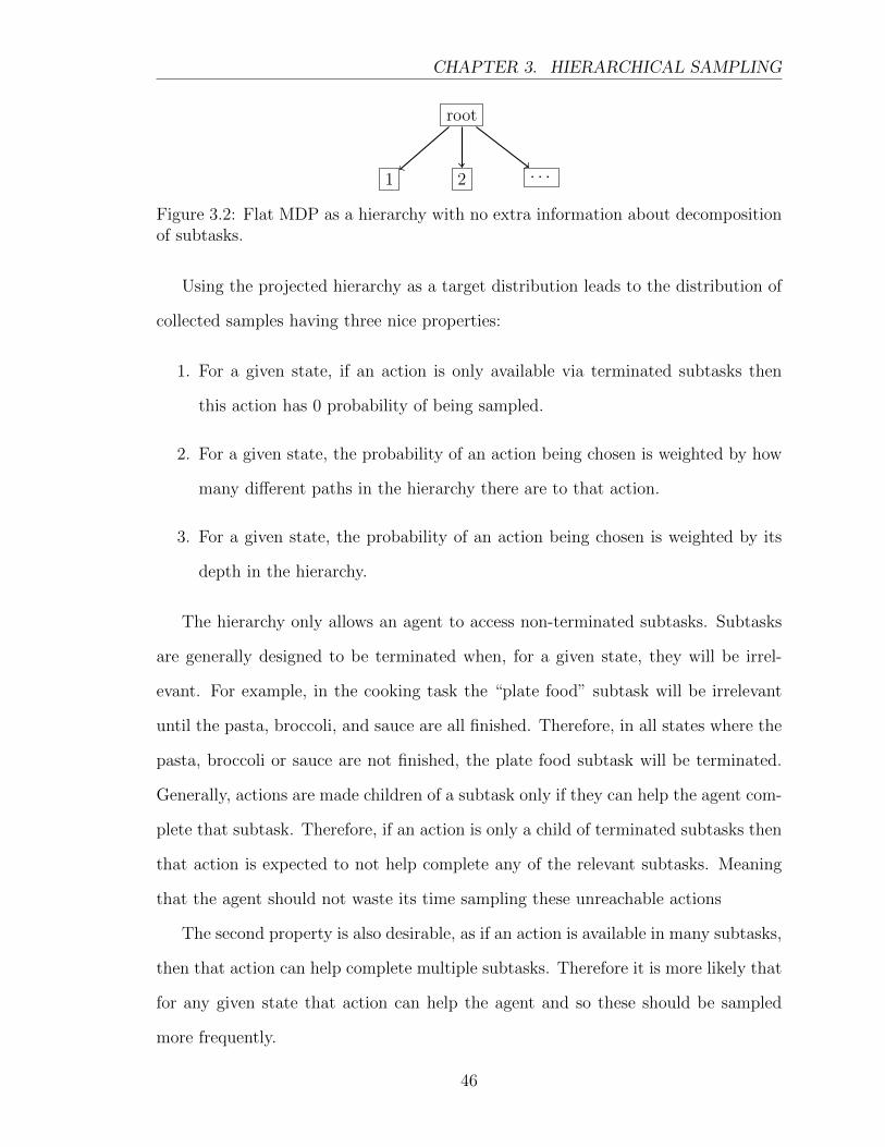
CHAPTER 3. HIERARCHICAL SAMPLING
root
1 2 · · ·
Figure 3.2: Flat MDP as a hierarchy with no extra information about decompositionof subtasks.
Using the projected hierarchy as a target distribution leads to the distribution of
collected samples having three nice properties:
1. For a given state, if an action is only available via terminated subtasks then
this action has 0 probability of being sampled.
2. For a given state, the probability of an action being chosen is weighted by how
many different paths in the hierarchy there are to that action.
3. For a given state, the probability of an action being chosen is weighted by its
depth in the hierarchy.
The hierarchy only allows an agent to access non-terminated subtasks. Subtasks
are generally designed to be terminated when, for a given state, they will be irrel-
evant. For example, in the cooking task the “plate food” subtask will be irrelevant
until the pasta, broccoli, and sauce are all finished. Therefore, in all states where the
pasta, broccoli or sauce are not finished, the plate food subtask will be terminated.
Generally, actions are made children of a subtask only if they can help the agent com-
plete that subtask. Therefore, if an action is only a child of terminated subtasks then
that action is expected to not help complete any of the relevant subtasks. Meaning
that the agent should not waste its time sampling these unreachable actions
The second property is also desirable, as if an action is available in many subtasks,
then that action can help complete multiple subtasks. Therefore it is more likely that
for any given state that action can help the agent and so these should be sampled
more frequently.
46
CHAPTER 3. HIERARCHICAL SAMPLING
The third property ensures that actions closer to the root subtask will be more
likely to be sampled. Remember that the root subtask has the goal of the original
MDP that was decomposed. Therefore an action closer to this subtask is more likely
to be helpful to completing the overall task, and not just one of the decomposed
subtasks. So it is more useful for these actions to be sampled more frequently.
It is important to note that this hierarchically projected distribution can be arbi-
trarily different from the flat uniform random sampling distribution. In states where
there are actions unreachable in the hierarchy, the unreachable actions will have 0
probability of being sampled, whereas in the flat uniform random distribution they
will have a non-zero probability. The weighting due to actions appearing multiple
times and an action’s depth in the hierarchy can make them different even in states
where there are no unreachable actions. If the hierarchy is poorly designed this can be
bad. For example if an important action for a state was unreachable in the hierarchy
the agent would never sample this action and therefore never learn that it should take
this action. In practice however, the hierarchies have been carefully designed by ex-
perts with prior knowledge and so this difference between the hierarchically projected
distribution and the flat uniform random distribution is not an issue.
The next sections describe the variations on the core sampling algorithm that
the agent uses to actually collect samples. The goal is that these action selection
strategies, select actions such that the distribution of samples over the state-action
space converge to the distribution defined by the hierarchical projection operation
from this section.
3.3.2 Hierarchy Sampling Algorithm
In section 2.6, I presented the LSPI algorithm. The key input to the LSPI algorithm
was the set of samples, D. The agent uses this sampling algorithm to produce the
sample set, D, that LSPI uses. No modifications to LSPI need to be made in order
47
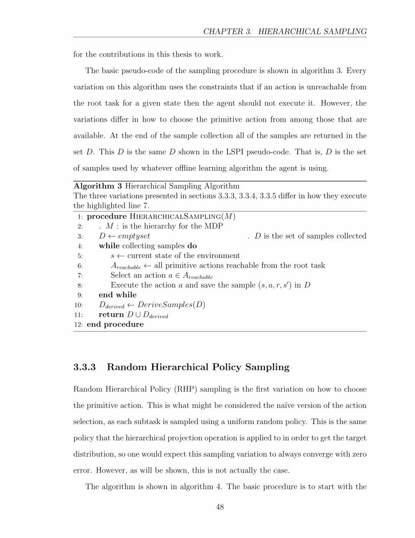
CHAPTER 3. HIERARCHICAL SAMPLING
for the contributions in this thesis to work.
The basic pseudo-code of the sampling procedure is shown in algorithm 3. Every
variation on this algorithm uses the constraints that if an action is unreachable from
the root task for a given state then the agent should not execute it. However, the
variations differ in how to choose the primitive action from among those that are
available. At the end of the sample collection all of the samples are returned in the
set D. This D is the same D shown in the LSPI pseudo-code. That is, D is the set
of samples used by whatever offline learning algorithm the agent is using.
Algorithm 3 Hierarchical Sampling AlgorithmThe three variations presented in sections 3.3.3, 3.3.4, 3.3.5 differ in how they executethe highlighted line 7.
1: procedure HierarchicalSampling(M)2: . M : is the hierarchy for the MDP3: D ← emptyset . D is the set of samples collected4: while collecting samples do5: s← current state of the environment6: Areachable ← all primitive actions reachable from the root task7: Select an action a ∈ Areachable8: Execute the action a and save the sample (s, a, r, s′) in D9: end while10: Dderived ← DeriveSamples(D)11: return D ∪Dderived
12: end procedure
3.3.3 Random Hierarchical Policy Sampling
Random Hierarchical Policy (RHP) sampling is the first variation on how to choose
the primitive action. This is what might be considered the naıve version of the action
selection, as each subtask is sampled using a uniform random policy. This is the same
policy that the hierarchical projection operation is applied to in order to get the target
distribution, so one would expect this sampling variation to always converge with zero
error. However, as will be shown, this is not actually the case.
The algorithm is shown in algorithm 4. The basic procedure is to start with the
48
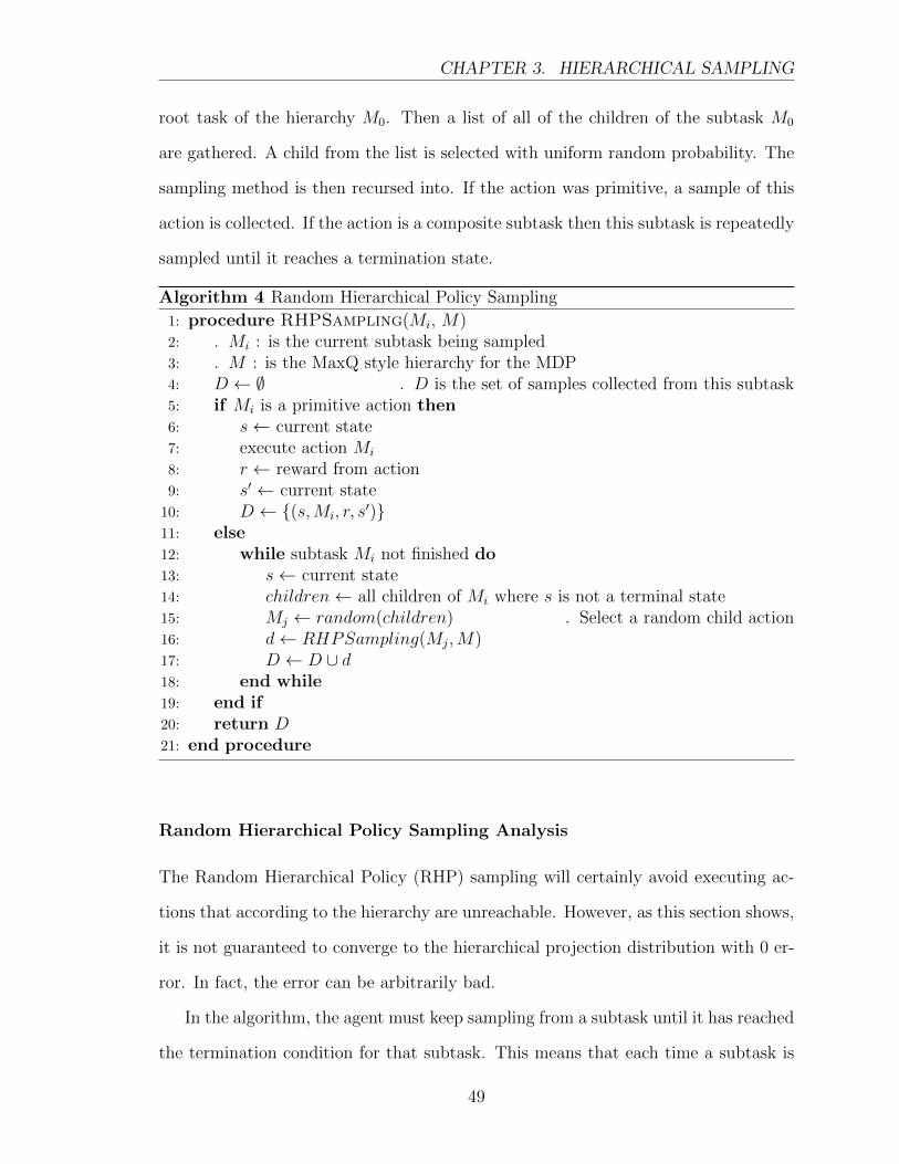
CHAPTER 3. HIERARCHICAL SAMPLING
root task of the hierarchy M0. Then a list of all of the children of the subtask M0
are gathered. A child from the list is selected with uniform random probability. The
sampling method is then recursed into. If the action was primitive, a sample of this
action is collected. If the action is a composite subtask then this subtask is repeatedly
sampled until it reaches a termination state.
Algorithm 4 Random Hierarchical Policy Sampling
1: procedure RHPSampling(Mi, M)2: . Mi : is the current subtask being sampled3: . M : is the MaxQ style hierarchy for the MDP4: D ← ∅ . D is the set of samples collected from this subtask5: if Mi is a primitive action then6: s← current state7: execute action Mi
8: r ← reward from action9: s′ ← current state10: D ← {(s,Mi, r, s
′)}11: else12: while subtask Mi not finished do13: s← current state14: children← all children of Mi where s is not a terminal state15: Mj ← random(children) . Select a random child action16: d← RHPSampling(Mj,M)17: D ← D ∪ d18: end while19: end if20: return D21: end procedure
Random Hierarchical Policy Sampling Analysis
The Random Hierarchical Policy (RHP) sampling will certainly avoid executing ac-
tions that according to the hierarchy are unreachable. However, as this section shows,
it is not guaranteed to converge to the hierarchical projection distribution with 0 er-
ror. In fact, the error can be arbitrarily bad.
In the algorithm, the agent must keep sampling from a subtask until it has reached
the termination condition for that subtask. This means that each time a subtask is
49
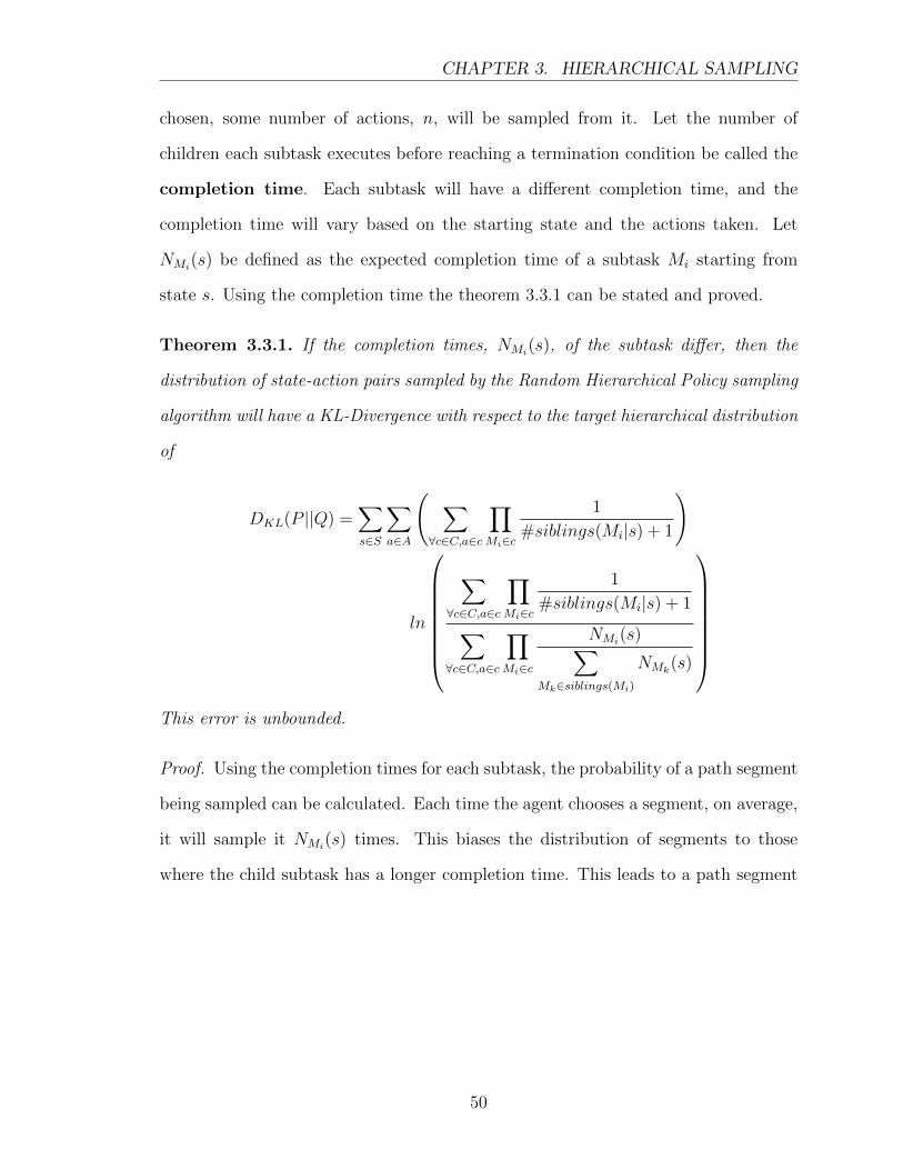
CHAPTER 3. HIERARCHICAL SAMPLING
chosen, some number of actions, n, will be sampled from it. Let the number of
children each subtask executes before reaching a termination condition be called the
completion time. Each subtask will have a different completion time, and the
completion time will vary based on the starting state and the actions taken. Let
NMi(s) be defined as the expected completion time of a subtask Mi starting from
state s. Using the completion time the theorem 3.3.1 can be stated and proved.
Theorem 3.3.1. If the completion times, NMi(s), of the subtask differ, then the
distribution of state-action pairs sampled by the Random Hierarchical Policy sampling
algorithm will have a KL-Divergence with respect to the target hierarchical distribution
of
DKL(P ||Q) =∑s∈S
∑a∈A
( ∑∀c∈C,a∈c
∏Mi∈c
1
#siblings(Mi|s) + 1
)
ln
∑
∀c∈C,a∈c
∏Mi∈c
1
#siblings(Mi|s) + 1∑∀c∈C,a∈c
∏Mi∈c
NMi(s)∑
Mk∈siblings(Mi)
NMk(s)
This error is unbounded.
Proof. Using the completion times for each subtask, the probability of a path segment
being sampled can be calculated. Each time the agent chooses a segment, on average,
it will sample it NMi(s) times. This biases the distribution of segments to those
where the child subtask has a longer completion time. This leads to a path segment
50
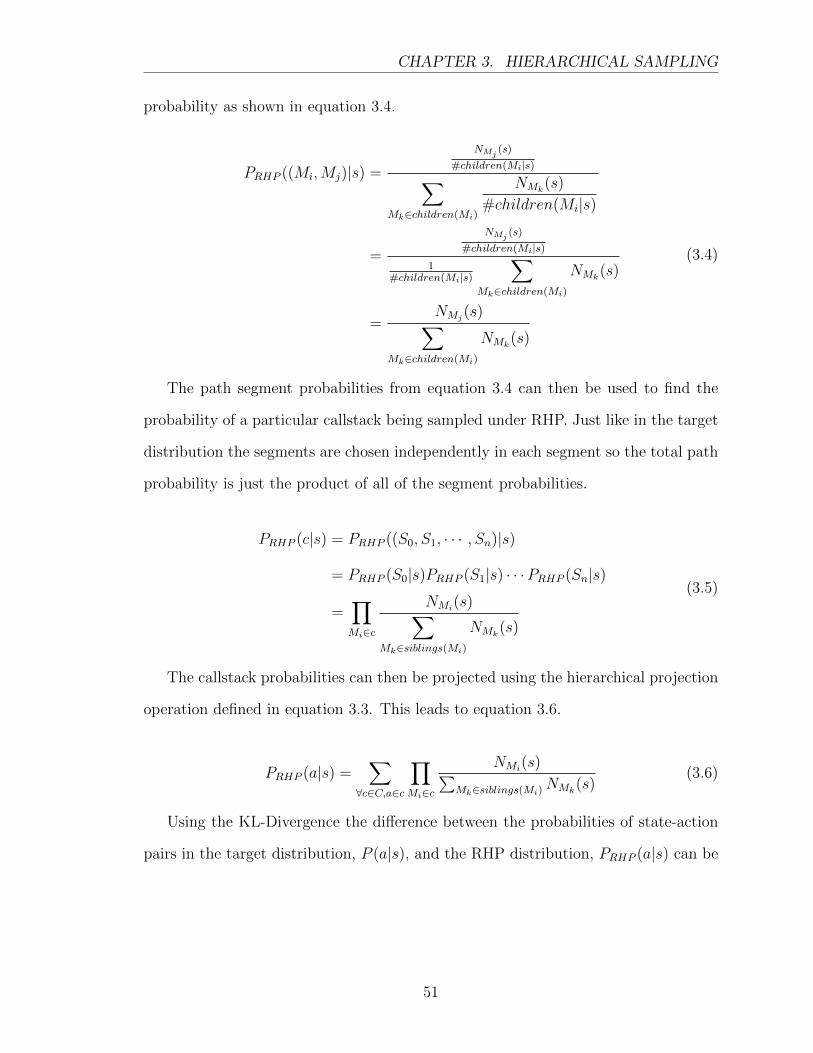
CHAPTER 3. HIERARCHICAL SAMPLING
probability as shown in equation 3.4.
PRHP ((Mi,Mj)|s) =
NMj(s)
#children(Mi|s)∑Mk∈children(Mi)
NMk(s)
#children(Mi|s)
=
NMj(s)
#children(Mi|s)1
#children(Mi|s)
∑Mk∈children(Mi)
NMk(s)
=NMj
(s)∑Mk∈children(Mi)
NMk(s)
(3.4)
The path segment probabilities from equation 3.4 can then be used to find the
probability of a particular callstack being sampled under RHP. Just like in the target
distribution the segments are chosen independently in each segment so the total path
probability is just the product of all of the segment probabilities.
PRHP (c|s) = PRHP ((S0, S1, · · · , Sn)|s)
= PRHP (S0|s)PRHP (S1|s) · · ·PRHP (Sn|s)
=∏Mi∈c
NMi(s)∑
Mk∈siblings(Mi)
NMk(s)
(3.5)
The callstack probabilities can then be projected using the hierarchical projection
operation defined in equation 3.3. This leads to equation 3.6.
PRHP (a|s) =∑
∀c∈C,a∈c
∏Mi∈c
NMi(s)∑
Mk∈siblings(Mi)NMk
(s)(3.6)
Using the KL-Divergence the difference between the probabilities of state-action
pairs in the target distribution, P (a|s), and the RHP distribution, PRHP (a|s) can be
51
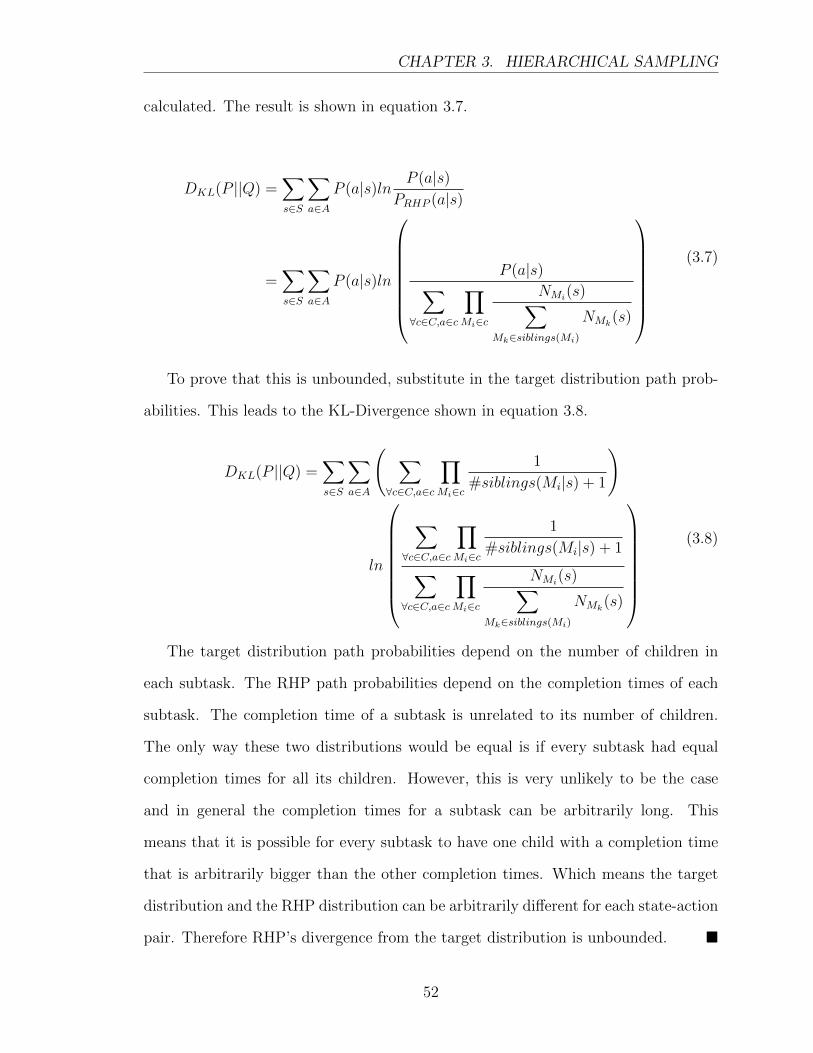
CHAPTER 3. HIERARCHICAL SAMPLING
calculated. The result is shown in equation 3.7.
DKL(P ||Q) =∑s∈S
∑a∈A
P (a|s)ln P (a|s)PRHP (a|s)
=∑s∈S
∑a∈A
P (a|s)ln
P (a|s)∑
∀c∈C,a∈c
∏Mi∈c
NMi(s)∑
Mk∈siblings(Mi)
NMk(s)
(3.7)
To prove that this is unbounded, substitute in the target distribution path prob-
abilities. This leads to the KL-Divergence shown in equation 3.8.
DKL(P ||Q) =∑s∈S
∑a∈A
( ∑∀c∈C,a∈c
∏Mi∈c
1
#siblings(Mi|s) + 1
)
ln
∑
∀c∈C,a∈c
∏Mi∈c
1
#siblings(Mi|s) + 1∑∀c∈C,a∈c
∏Mi∈c
NMi(s)∑
Mk∈siblings(Mi)
NMk(s)
(3.8)
The target distribution path probabilities depend on the number of children in
each subtask. The RHP path probabilities depend on the completion times of each
subtask. The completion time of a subtask is unrelated to its number of children.
The only way these two distributions would be equal is if every subtask had equal
completion times for all its children. However, this is very unlikely to be the case
and in general the completion times for a subtask can be arbitrarily long. This
means that it is possible for every subtask to have one child with a completion time
that is arbitrarily bigger than the other completion times. Which means the target
distribution and the RHP distribution can be arbitrarily different for each state-action
pair. Therefore RHP’s divergence from the target distribution is unbounded. �
52
CHAPTER 3. HIERARCHICAL SAMPLING
3.3.4 Weakly Polled Sampling
The issue with RHP sampling is that, in some cases, it can focus its sample collection
too heavily on a single subtask. Sticking with subtasks until they terminate can skew
the distribution of samples towards subtasks that take a long time to complete when
randomly sampling. Weakly polled sampling attempts to fix this issue through a
minor change to the primitive action selection procedure.
Rather than sticking with a subtask to completion, weakly polled sampling adds
an extra “exit subtask” action to every subtask. Each time the agent selects an action
in a subtask it has the chance of selecting the exit subtask action which kicks the
agent back up to the parent subtask. The modified pseudocode for this is shown in
algorithm 5.
The relevant changes are on lines 15 and 16-18. Line 15 modifies the action
selection to select an action from the union of the set of children actions and the
early exit action. Lines 16-18 ensure that if the early exit action was chosen then it
will leave the function early. Otherwise the algorithm is exactly the same as the RHP
Sampling.
53
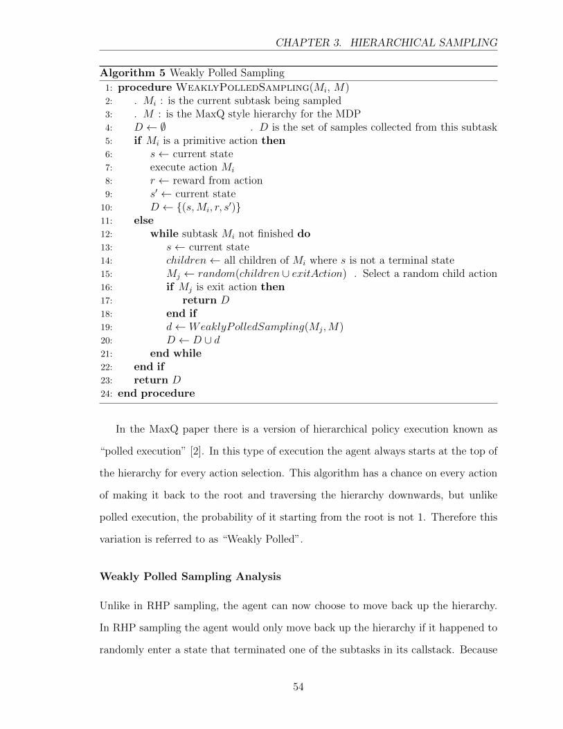
CHAPTER 3. HIERARCHICAL SAMPLING
Algorithm 5 Weakly Polled Sampling
1: procedure WeaklyPolledSampling(Mi, M)2: . Mi : is the current subtask being sampled3: . M : is the MaxQ style hierarchy for the MDP4: D ← ∅ . D is the set of samples collected from this subtask5: if Mi is a primitive action then6: s← current state7: execute action Mi
8: r ← reward from action9: s′ ← current state10: D ← {(s,Mi, r, s
′)}11: else12: while subtask Mi not finished do13: s← current state14: children← all children of Mi where s is not a terminal state15: Mj ← random(children ∪ exitAction) . Select a random child action16: if Mj is exit action then17: return D18: end if19: d← WeaklyPolledSampling(Mj,M)20: D ← D ∪ d21: end while22: end if23: return D24: end procedure
In the MaxQ paper there is a version of hierarchical policy execution known as
“polled execution” [2]. In this type of execution the agent always starts at the top of
the hierarchy for every action selection. This algorithm has a chance on every action
of making it back to the root and traversing the hierarchy downwards, but unlike
polled execution, the probability of it starting from the root is not 1. Therefore this
variation is referred to as “Weakly Polled”.
Weakly Polled Sampling Analysis
Unlike in RHP sampling, the agent can now choose to move back up the hierarchy.
In RHP sampling the agent would only move back up the hierarchy if it happened to
randomly enter a state that terminated one of the subtasks in its callstack. Because
54
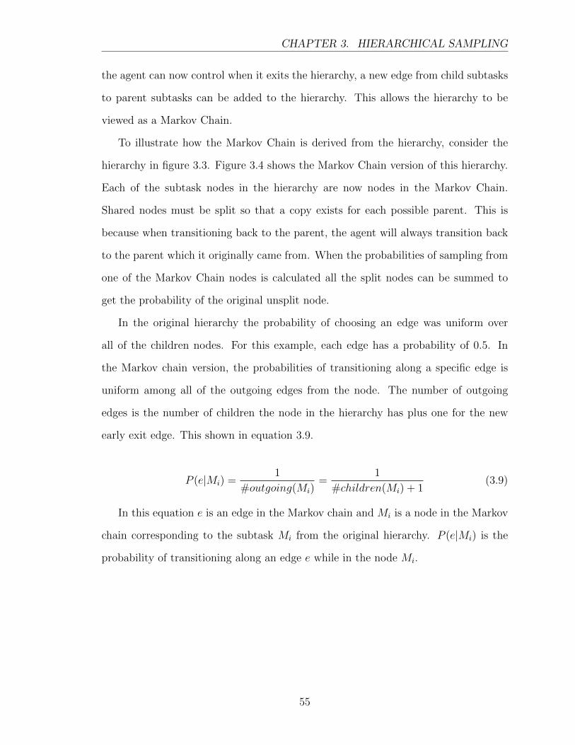
CHAPTER 3. HIERARCHICAL SAMPLING
the agent can now control when it exits the hierarchy, a new edge from child subtasks
to parent subtasks can be added to the hierarchy. This allows the hierarchy to be
viewed as a Markov Chain.
To illustrate how the Markov Chain is derived from the hierarchy, consider the
hierarchy in figure 3.3. Figure 3.4 shows the Markov Chain version of this hierarchy.
Each of the subtask nodes in the hierarchy are now nodes in the Markov Chain.
Shared nodes must be split so that a copy exists for each possible parent. This is
because when transitioning back to the parent, the agent will always transition back
to the parent which it originally came from. When the probabilities of sampling from
one of the Markov Chain nodes is calculated all the split nodes can be summed to
get the probability of the original unsplit node.
In the original hierarchy the probability of choosing an edge was uniform over
all of the children nodes. For this example, each edge has a probability of 0.5. In
the Markov chain version, the probabilities of transitioning along a specific edge is
uniform among all of the outgoing edges from the node. The number of outgoing
edges is the number of children the node in the hierarchy has plus one for the new
early exit edge. This shown in equation 3.9.
P (e|Mi) =1
#outgoing(Mi)=
1
#children(Mi) + 1(3.9)
In this equation e is an edge in the Markov chain and Mi is a node in the Markov
chain corresponding to the subtask Mi from the original hierarchy. P (e|Mi) is the
probability of transitioning along an edge e while in the node Mi.
55
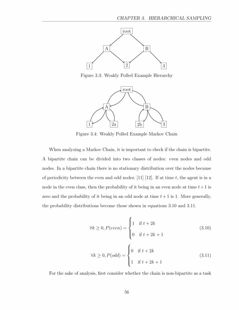
CHAPTER 3. HIERARCHICAL SAMPLING
root
A B
1 2 3
Figure 3.3: Weakly Polled Example Hierarchy
root
A B
1 2a 2b 3
Figure 3.4: Weakly Polled Example Markov Chain
When analyzing a Markov Chain, it is important to check if the chain is bipartite.
A bipartite chain can be divided into two classes of nodes: even nodes and odd
nodes. In a bipartite chain there is no stationary distribution over the nodes because
of periodicity between the even and odd nodes. [11] [12]. If at time t, the agent is in a
node in the even class, then the probability of it being in an even node at time t+1 is
zero and the probability of it being in an odd node at time t+ 1 is 1. More generally,
the probability distributions become those shown in equations 3.10 and 3.11.
∀k ≥ 0, P (even) =
1 if t+ 2k
0 if t+ 2k + 1
(3.10)
∀k ≥ 0, P (odd) =
0 if t+ 2k
1 if t+ 2k + 1
(3.11)
For the sake of analysis, first consider whether the chain is non-bipartite as a task
56
CHAPTER 3. HIERARCHICAL SAMPLING
hierarchy can be either bipartite or non-bipartite. 1 If a hierarchy is bipartite, then
the nodes can be split into their even and odd classes and then analyzed using the
same non-bipartite Markov Chain stationary distribution equations.
For a non-bipartite Markov chain, the stationary distribution over the states is
defined by the simple formula [11] [12] shown in equation 3.12.
ω(v) =C(v)
k(3.12)
Where v is a node in the Markov Chain, this case v ∈M . C(v) is the total of the
edge weights for all edges between node v and some other node, and k =∑
v∈V C(v).
Theorem 3.3.2. The distribution over the state-action pairs sampled by the Weakly
Polled sampling algorithm will have a KL-Divergence with respect to the target hier-
archical projection distribution of
DKL(P ||Q) =∑s∈S
∑a∈A
∑Ma∈parent(a)
P (Ma|s)#children(Ma|s)
ln
∑Ma∈parent(a)
P (Ma|s)∑
x∈A∑
Mx∈parent(x)1
#children(Mx|s)+1
#children(Ma|s)∑
Ma∈parent(a)1
#children(Ma|s)+1
(3.13)
when the task hierarchy is non-bipartite. When the task hierarchy is bipartite, the
KL-Divergence with respect to the target hierarchical projection distribution will be
1Most task hierarchies, being poly-trees will be bipartite. However, it is possible to imagine non-bipartite hierarchies. For example, consider a hierarchy with a root node that has two children: acomposite task A and a primitive task b. If A also has b as a child, then the graph is non-bipartite.
57
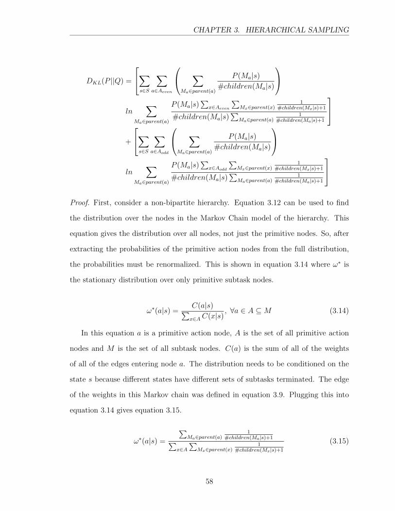
CHAPTER 3. HIERARCHICAL SAMPLING
DKL(P ||Q) =
∑s∈S
∑a∈Aeven
∑Ma∈parent(a)
P (Ma|s)#children(Ma|s)
ln
∑Ma∈parent(a)
P (Ma|s)∑
x∈Aeven
∑Mx∈parent(x)
1#children(Mx|s)+1
#children(Ma|s)∑
Ma∈parent(a)1
#children(Ma|s)+1
+
∑s∈S
∑a∈Aodd
∑Ma∈parent(a)
P (Ma|s)#children(Ma|s)
ln
∑Ma∈parent(a)
P (Ma|s)∑
x∈Aodd
∑Mx∈parent(x)
1#children(Mx|s)+1
#children(Ma|s)∑
Ma∈parent(a)1
#children(Ma|s)+1
Proof. First, consider a non-bipartite hierarchy. Equation 3.12 can be used to find
the distribution over the nodes in the Markov Chain model of the hierarchy. This
equation gives the distribution over all nodes, not just the primitive nodes. So, after
extracting the probabilities of the primitive action nodes from the full distribution,
the probabilities must be renormalized. This is shown in equation 3.14 where ω∗ is
the stationary distribution over only primitive subtask nodes.
ω∗(a|s) =C(a|s)∑x∈AC(x|s)
, ∀a ∈ A ⊆M (3.14)
In this equation a is a primitive action node, A is the set of all primitive action
nodes and M is the set of all subtask nodes. C(a) is the sum of all of the weights
of all of the edges entering node a. The distribution needs to be conditioned on the
state s because different states have different sets of subtasks terminated. The edge
of the weights in this Markov chain was defined in equation 3.9. Plugging this into
equation 3.14 gives equation 3.15.
ω∗(a|s) =
∑Ma∈parent(a)
1#children(Ma|s)+1∑
x∈A∑
Mx∈parent(x)1
#children(Mx|s)+1
(3.15)
58
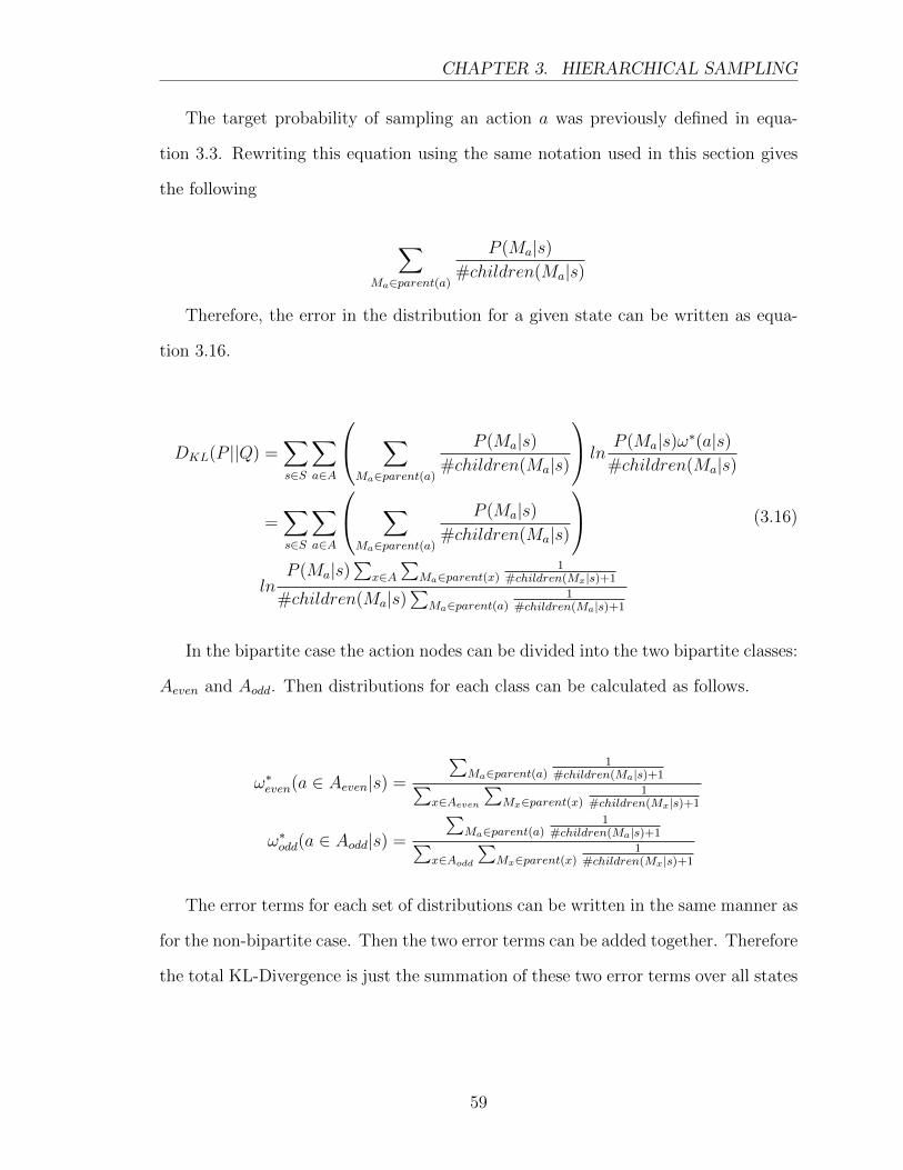
CHAPTER 3. HIERARCHICAL SAMPLING
The target probability of sampling an action a was previously defined in equa-
tion 3.3. Rewriting this equation using the same notation used in this section gives
the following
∑Ma∈parent(a)
P (Ma|s)#children(Ma|s)
Therefore, the error in the distribution for a given state can be written as equa-
tion 3.16.
DKL(P ||Q) =∑s∈S
∑a∈A
∑Ma∈parent(a)
P (Ma|s)#children(Ma|s)
lnP (Ma|s)ω∗(a|s)
#children(Ma|s)
=∑s∈S
∑a∈A
∑Ma∈parent(a)
P (Ma|s)#children(Ma|s)
ln
P (Ma|s)∑
x∈A∑
Ma∈parent(x)1
#children(Mx|s)+1
#children(Ma|s)∑
Ma∈parent(a)1
#children(Ma|s)+1
(3.16)
In the bipartite case the action nodes can be divided into the two bipartite classes:
Aeven and Aodd. Then distributions for each class can be calculated as follows.
ω∗even(a ∈ Aeven|s) =
∑Ma∈parent(a)
1#children(Ma|s)+1∑
x∈Aeven
∑Mx∈parent(x)
1#children(Mx|s)+1
ω∗odd(a ∈ Aodd|s) =
∑Ma∈parent(a)
1#children(Ma|s)+1∑
x∈Aodd
∑Mx∈parent(x)
1#children(Mx|s)+1
The error terms for each set of distributions can be written in the same manner as
for the non-bipartite case. Then the two error terms can be added together. Therefore
the total KL-Divergence is just the summation of these two error terms over all states
59
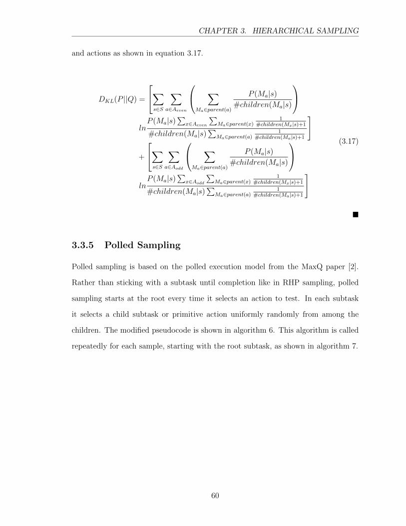
CHAPTER 3. HIERARCHICAL SAMPLING
and actions as shown in equation 3.17.
DKL(P ||Q) =
∑s∈S
∑a∈Aeven
∑Ma∈parent(a)
P (Ma|s)#children(Ma|s)
lnP (Ma|s)
∑x∈Aeven
∑Ma∈parent(x)
1#children(Mx|s)+1
#children(Ma|s)∑
Ma∈parent(a)1
#children(Ma|s)+1
]
+
∑s∈S
∑a∈Aodd
∑Ma∈parent(a)
P (Ma|s)#children(Ma|s)
lnP (Ma|s)
∑x∈Aodd
∑Ma∈parent(x)
1#children(Mx|s)+1
#children(Ma|s)∑
Ma∈parent(a)1
#children(Ma|s)+1
](3.17)
�
3.3.5 Polled Sampling
Polled sampling is based on the polled execution model from the MaxQ paper [2].
Rather than sticking with a subtask until completion like in RHP sampling, polled
sampling starts at the root every time it selects an action to test. In each subtask
it selects a child subtask or primitive action uniformly randomly from among the
children. The modified pseudocode is shown in algorithm 6. This algorithm is called
repeatedly for each sample, starting with the root subtask, as shown in algorithm 7.
60
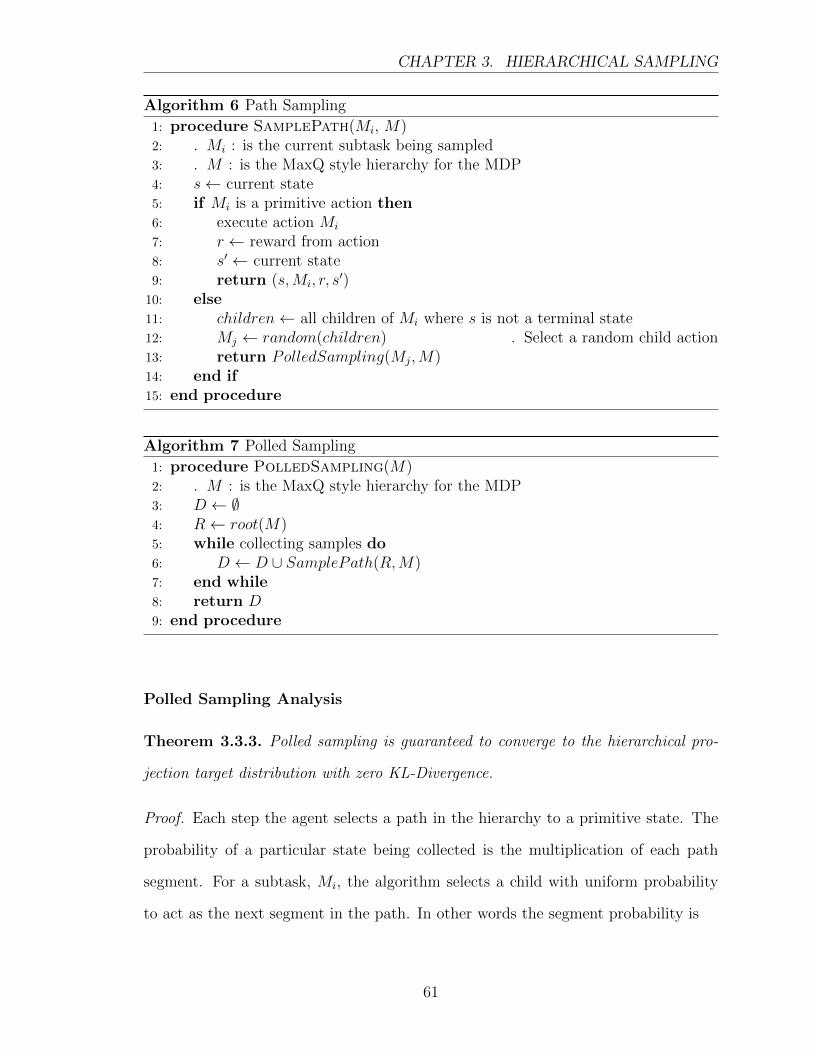
CHAPTER 3. HIERARCHICAL SAMPLING
Algorithm 6 Path Sampling
1: procedure SamplePath(Mi, M)2: . Mi : is the current subtask being sampled3: . M : is the MaxQ style hierarchy for the MDP4: s← current state5: if Mi is a primitive action then6: execute action Mi
7: r ← reward from action8: s′ ← current state9: return (s,Mi, r, s
′)10: else11: children← all children of Mi where s is not a terminal state12: Mj ← random(children) . Select a random child action13: return PolledSampling(Mj,M)14: end if15: end procedure
Algorithm 7 Polled Sampling
1: procedure PolledSampling(M)2: . M : is the MaxQ style hierarchy for the MDP3: D ← ∅4: R← root(M)5: while collecting samples do6: D ← D ∪ SamplePath(R,M)7: end while8: return D9: end procedure
Polled Sampling Analysis
Theorem 3.3.3. Polled sampling is guaranteed to converge to the hierarchical pro-
jection target distribution with zero KL-Divergence.
Proof. Each step the agent selects a path in the hierarchy to a primitive state. The
probability of a particular state being collected is the multiplication of each path
segment. For a subtask, Mi, the algorithm selects a child with uniform probability
to act as the next segment in the path. In other words the segment probability is
61
CHAPTER 3. HIERARCHICAL SAMPLING
1
#children(Mi|s)
This is the same probability as a path segment in the hierarchical projection
distribution. This probability was defined in equation 3.1. Therefore, the probability
of any one path being picked for an action is equal to the hierarchical projection
distribution path probability defined in equation 3.2. For a given state, each time
a path is chosen, it is chosen independently and because the distribution does not
change, it is guaranteed that the distribution of sampled paths will converge to the
theoretical hierarchical distribution.
Just like in the hierarchical projection operation, the actions actually being sam-
pled are the primitive action subtasks at the end of each path. Therefore the prob-
ability of an action picked via polled sampling is the same as the target hierarchical
projection probability defined in equation 3.3. �
3.3.6 Discussion
The previous sections presented the main hierarchical sampling algorithm and three
different variations on this algorithm. Out of the three, only one of the algorithms is
guaranteed to converge with zero KL-Divergence from the target distribution. How-
ever, it is important to note that this result is only about asymptotic convergence.
I did not perform a finite sample analysis. So nothing theoretical can be said about
the rate at which these algorithms converge to their final distributions. Because the
rates of convergence are unknown, it is difficult to say that the polled sampling will
always perform best. There may be situations where weakly polled sampling, or RHP
sampling converges faster. Even though they will converge with error, it might be
possible for the error to be small enough, such that LSPI can find the optimal policy.
Also, there may be other variations that perform even better.
62
CHAPTER 3. HIERARCHICAL SAMPLING
It also cannot be said how much error in the sample distribution is enough to
break the policy solver that uses the collected samples. It may be that on some
domains RHP has an error small enough for the agent to find an optimal policy. On
other domains the error may be so large that the policies found via RHP sampling
perform worse than flat LSPI. For these two reasons it is important to empirically
evaluate the performance of all three variations.
3.4 Derived Samples
This section presents two methods for expanding the set of collected samples using
the hierarchy. These generated samples are referred to as “derived samples” because
the agent creates them by examining the real samples in the context of the given task
hierarchy. The first type of derived samples presented are inhibited action samples.
These samples are designed to guarantee that the policy does not choose an action
prohibited by the hierarchy. The second type of hierarchy samples are abstract sam-
ples. These samples use state abstraction in the hierarchy to generate extra samples
for potentially unvisited state-action pairs.
3.4.1 Inhibited Action Samples
When using the hierarchical sampling algorithm, no matter the variation, the distri-
bution of samples over the state-action space is guaranteed to contain no state-action
pairs where in the given state there is no path in the hierarchy to the action through
non-terminated tasks. This property is desirable because it prevents the agent from
wasting samples on irrelevant actions and in some cases can be used to prevent the
agent from taking dangerous actions. However, the issue is that the learning algo-
rithm using these samples is unaware of the hierarchy. In some cases the policy solver
can decide that these unsampled actions are the best action to use in the policy.
63
CHAPTER 3. HIERARCHICAL SAMPLING
To resolve this issue, a way is needed to inform the learning agent that the inhibited
actions should never be chosen for the policy. This has to be done in such a way that
the choice of the optimal action from among the other actions is unaffected.
Inhibited action samples are generated by combining the collected samples with
information in the hierarchy. For each sample that was collected, the agent can
consult its hierarchy to see if there are any unreachable actions. If there are such
actions, then for each action a new sample is generated. This new sample has the
same s and s′ as the original sample, and the action is set to the unreachable action.
The only remaining portion to be determined is the reward.
It is important to properly choose the reward that is assigned to the generated
samples. If the reward is higher than any of the action rewards, then there is a
chance the policy will choose the inhibited action. If the reward is higher than the
real samples then it can affect the estimate of the value of the state thus causing
inaccuracies in other parts of the policy. Therefore, it is necessary to choose a reward
that is less than or equal to the worst possible value of a state-action pair in the
MDP.
The worst possible value a state-action pair could have, is if the policy chose an
action that does not change the state and has the smallest reward out of all of the
actions. This means that when following the policy, the agent would execute this
action an infinite number of times receiving the reward rmin each time. The total
reward collected from following the policy in this state is then defined by the sum
of the discounted rewards. This happens to be a geometric series, so a closed form
64
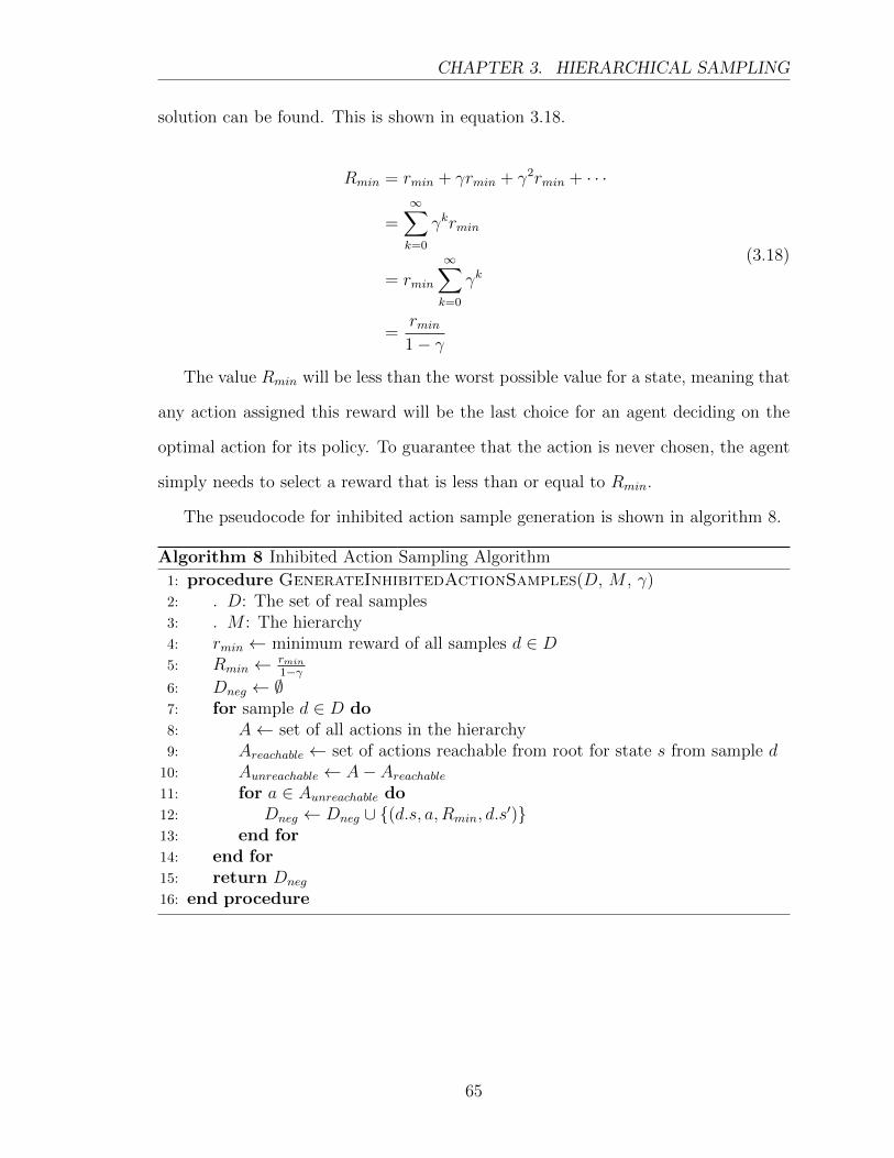
CHAPTER 3. HIERARCHICAL SAMPLING
solution can be found. This is shown in equation 3.18.
Rmin = rmin + γrmin + γ2rmin + · · ·
=∞∑k=0
γkrmin
= rmin
∞∑k=0
γk
=rmin1− γ
(3.18)
The value Rmin will be less than the worst possible value for a state, meaning that
any action assigned this reward will be the last choice for an agent deciding on the
optimal action for its policy. To guarantee that the action is never chosen, the agent
simply needs to select a reward that is less than or equal to Rmin.
The pseudocode for inhibited action sample generation is shown in algorithm 8.
Algorithm 8 Inhibited Action Sampling Algorithm
1: procedure GenerateInhibitedActionSamples(D, M , γ)2: . D: The set of real samples3: . M : The hierarchy4: rmin ← minimum reward of all samples d ∈ D5: Rmin ← rmin
1−γ6: Dneg ← ∅7: for sample d ∈ D do8: A← set of all actions in the hierarchy9: Areachable ← set of actions reachable from root for state s from sample d10: Aunreachable ← A− Areachable11: for a ∈ Aunreachable do12: Dneg ← Dneg ∪ {(d.s, a, Rmin, d.s
′)}13: end for14: end for15: return Dneg
16: end procedure
65
CHAPTER 3. HIERARCHICAL SAMPLING
3.4.2 Abstract Samples
In many MDPs there are state variables in the state that only affect the value of a
small subset of the state-action space. Unfortunately, even though these state vari-
ables affect the transition and reward functions in only a small part of the state-action
space, the flat RL algorithms must spend time learning that these state variables are
largely irrelevant by sampling the MDP. One of the major advantages of the MaxQ
framework is that the hierarchical decomposition allows each subtask to have an ab-
stract state function. This function can remove the irrelevant state variables, so that
the subtask policy ignores the irrelevant variables. This can significantly shrink each
subtask’s state-action space and thus make it much easier to learn the optimal policy
in each subtask.
It would be ideal to take this same state abstraction and apply it in the flat MDP
case, so that the agent does not need to waste samples determining that a state
variable is irrelevant. Abstract samples provide a way to take the state abstraction
functions encoded in the MaxQ hierarchy and translate the information so that the
offline flat MDP algorithm can utilize it.
For each real sample collected, the sample is checked against the hierarchy to
see if there are any irrelevant state variables for the sample’s action. If there are any
irrelevant variables found, then the new abstract samples are generated by copying the
real sample and then randomly changing the values of the irrelevant state variables.
These abstract samples teach the offline learning algorithm that the transition and
reward function are unaffected by the irrelevant variables without requiring the agent
to collect explicit samples from the environment, like it would in the normal flat RL
algorithms.
MaxQ uses many different state abstraction rules, but the one that allows abstract
samples to be generated is the “Max Node Irrelevance” condition [2]. Assume that the
state can be factored into the set of relevant state variables, X, and irrelevant state
66
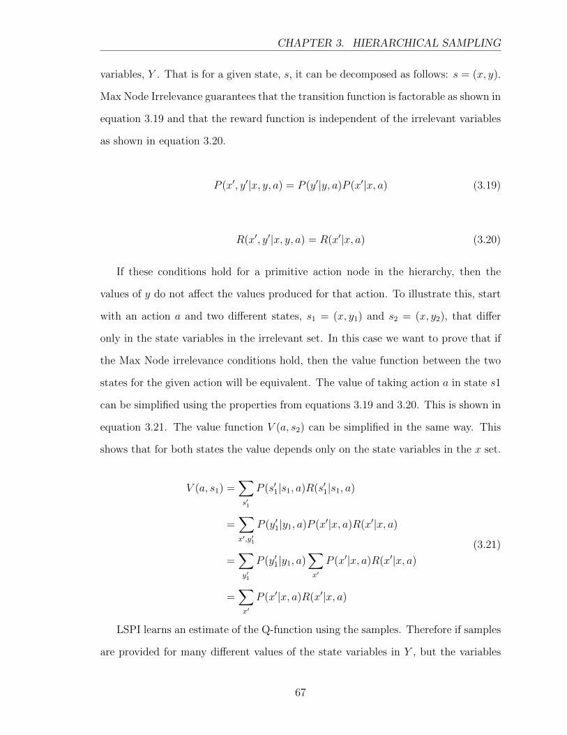
CHAPTER 3. HIERARCHICAL SAMPLING
variables, Y . That is for a given state, s, it can be decomposed as follows: s = (x, y).
Max Node Irrelevance guarantees that the transition function is factorable as shown in
equation 3.19 and that the reward function is independent of the irrelevant variables
as shown in equation 3.20.
P (x′, y′|x, y, a) = P (y′|y, a)P (x′|x, a) (3.19)
R(x′, y′|x, y, a) = R(x′|x, a) (3.20)
If these conditions hold for a primitive action node in the hierarchy, then the
values of y do not affect the values produced for that action. To illustrate this, start
with an action a and two different states, s1 = (x, y1) and s2 = (x, y2), that differ
only in the state variables in the irrelevant set. In this case we want to prove that if
the Max Node irrelevance conditions hold, then the value function between the two
states for the given action will be equivalent. The value of taking action a in state s1
can be simplified using the properties from equations 3.19 and 3.20. This is shown in
equation 3.21. The value function V (a, s2) can be simplified in the same way. This
shows that for both states the value depends only on the state variables in the x set.
V (a, s1) =∑s′1
P (s′1|s1, a)R(s′1|s1, a)
=∑x′,y′1
P (y′1|y1, a)P (x′|x, a)R(x′|x, a)
=∑y′1
P (y′1|y1, a)∑x′
P (x′|x, a)R(x′|x, a)
=∑x′
P (x′|x, a)R(x′|x, a)
(3.21)
LSPI learns an estimate of the Q-function using the samples. Therefore if samples
are provided for many different values of the state variables in Y , but the variables
67
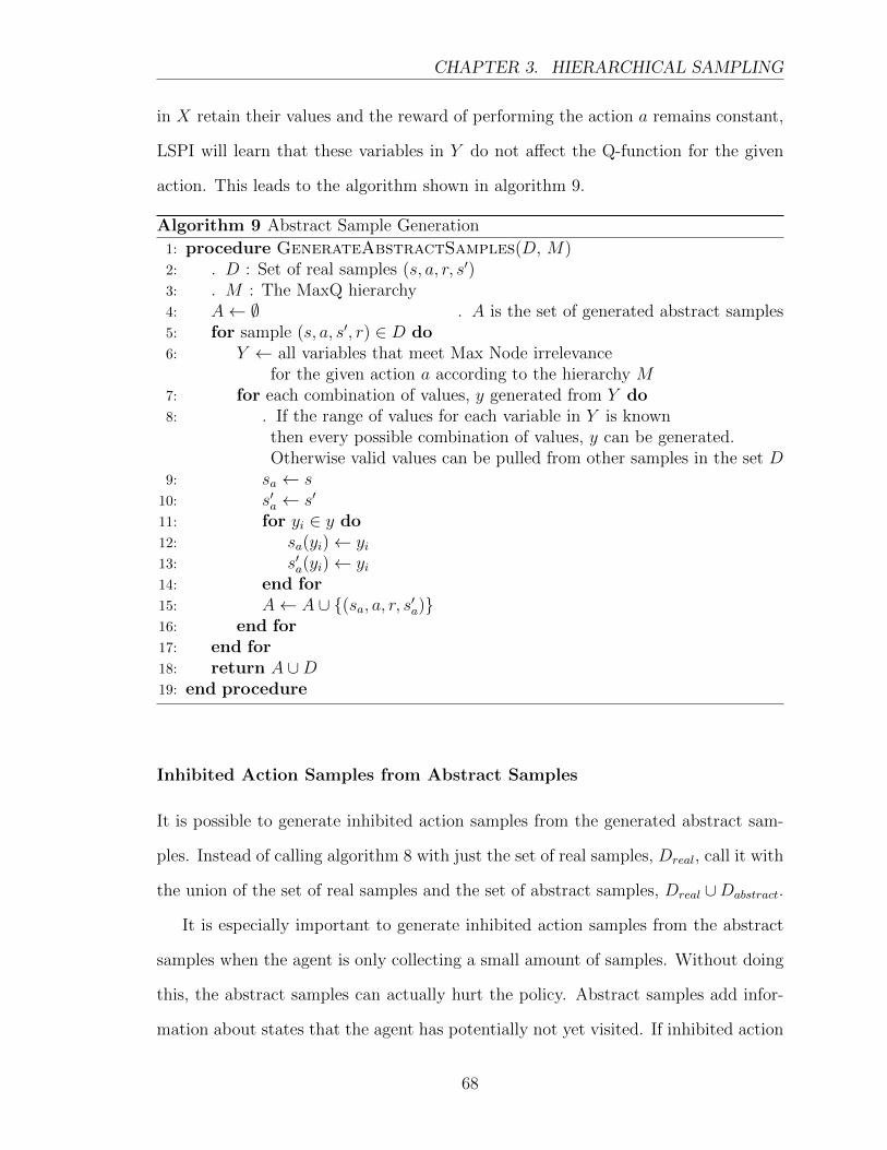
CHAPTER 3. HIERARCHICAL SAMPLING
in X retain their values and the reward of performing the action a remains constant,
LSPI will learn that these variables in Y do not affect the Q-function for the given
action. This leads to the algorithm shown in algorithm 9.
Algorithm 9 Abstract Sample Generation
1: procedure GenerateAbstractSamples(D, M)2: . D : Set of real samples (s, a, r, s′)3: . M : The MaxQ hierarchy4: A← ∅ . A is the set of generated abstract samples5: for sample (s, a, s′, r) ∈ D do6: Y ← all variables that meet Max Node irrelevance
for the given action a according to the hierarchy M7: for each combination of values, y generated from Y do8: . If the range of values for each variable in Y is known
then every possible combination of values, y can be generated.Otherwise valid values can be pulled from other samples in the set D
9: sa ← s10: s′a ← s′
11: for yi ∈ y do12: sa(yi)← yi13: s′a(yi)← yi14: end for15: A← A ∪ {(sa, a, r, s′a)}16: end for17: end for18: return A ∪D19: end procedure
Inhibited Action Samples from Abstract Samples
It is possible to generate inhibited action samples from the generated abstract sam-
ples. Instead of calling algorithm 8 with just the set of real samples, Dreal, call it with
the union of the set of real samples and the set of abstract samples, Dreal ∪Dabstract.
It is especially important to generate inhibited action samples from the abstract
samples when the agent is only collecting a small amount of samples. Without doing
this, the abstract samples can actually hurt the policy. Abstract samples add infor-
mation about states that the agent has potentially not yet visited. If inhibited action
68
CHAPTER 3. HIERARCHICAL SAMPLING
samples are only generated for real samples and not the derived abstract samples,
then there may be states which were never really sampled, but still have abstract
samples. In these states the inhibited action samples are required to guarantee that
LSPI does not get confused and choose an action that should be inhibited.
3.4.3 Discussion
Both of types of derived samples are going to skew the distribution of real samples.
This invalidates the sample convergence results, however, the target distribution is
clearly only a sufficient condition for convergence. If converging to the target dis-
tribution was necessary, then LSPI would not work with uniform random sampling.
Really, the most important thing for the convergence of LSPI, is that it receives
lots of high quality data about as many of the state-action pairs as possible. Both of
these techniques only add correct information to the existing real sample information.
Therefore it seems reasonable to expect that these techniques will help performance.
Even if the effects did lead to a distribution LSPI could not work with, the LSPI
algorithm contains a term to undo biasing in the sample distribution. This could
be used to fix any of the biases introduced by derived samples. Future work will
examine a more robust theoretical analysis of how both of these techniques affect the
convergence properties.
3.5 Hierarchical Sampling with Derived Samples
Algorithm 10 shows the full algorithm using both the hierarchical sampling varia-
tion and the derived sample generation subroutines. Note that the order that the
samples are generated is important. The abstract samples must be generated first
so that inhibited action samples can be generated for both the abstract samples and
the real samples. Also the LSPI algorithm could be replaced by another off-policy,
69
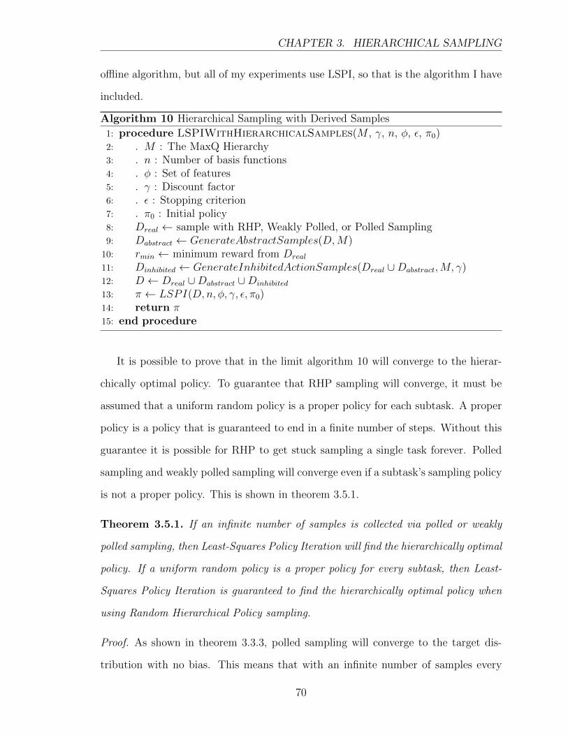
CHAPTER 3. HIERARCHICAL SAMPLING
offline algorithm, but all of my experiments use LSPI, so that is the algorithm I have
included.
Algorithm 10 Hierarchical Sampling with Derived Samples
1: procedure LSPIWithHierarchicalSamples(M , γ, n, φ, ε, π0)2: . M : The MaxQ Hierarchy3: . n : Number of basis functions4: . φ : Set of features5: . γ : Discount factor6: . ε : Stopping criterion7: . π0 : Initial policy8: Dreal ← sample with RHP, Weakly Polled, or Polled Sampling9: Dabstract ← GenerateAbstractSamples(D,M)10: rmin ← minimum reward from Dreal
11: Dinhibited ← GenerateInhibitedActionSamples(Dreal ∪Dabstract,M, γ)12: D ← Dreal ∪Dabstract ∪Dinhibited
13: π ← LSPI(D,n, φ, γ, ε, π0)14: return π15: end procedure
It is possible to prove that in the limit algorithm 10 will converge to the hierar-
chically optimal policy. To guarantee that RHP sampling will converge, it must be
assumed that a uniform random policy is a proper policy for each subtask. A proper
policy is a policy that is guaranteed to end in a finite number of steps. Without this
guarantee it is possible for RHP to get stuck sampling a single task forever. Polled
sampling and weakly polled sampling will converge even if a subtask’s sampling policy
is not a proper policy. This is shown in theorem 3.5.1.
Theorem 3.5.1. If an infinite number of samples is collected via polled or weakly
polled sampling, then Least-Squares Policy Iteration will find the hierarchically optimal
policy. If a uniform random policy is a proper policy for every subtask, then Least-
Squares Policy Iteration is guaranteed to find the hierarchically optimal policy when
using Random Hierarchical Policy sampling.
Proof. As shown in theorem 3.3.3, polled sampling will converge to the target dis-
tribution with no bias. This means that with an infinite number of samples every
70
CHAPTER 3. HIERARCHICAL SAMPLING
reachable path in every state will be sampled. Therefore, every state-action pair pos-
sible is sampled with polled sampling. With an infinite amount of samples, each of
these state-action pairs is sampled an infinite amount of times.
The Q-learning paper [17] showed that if every state-action pair is visited infinitely
often then it is possible for the agent to find the optimal policy. In this case only
state-action pairs allowed by the hierarchy are sampled infinitely often, so globally
optimal policies cannot be guaranteed. However, hierarchically optimal policies can
be guaranteed because all of the state-action pairs consistent with the hierarchy will
be sampled infinitely often.
Weakly polled sampling will have bias from the target distribution, but it has a
non-zero probability of sampling any reachable action for a given state. Therefore,
with an infinite amount of samples, weakly polled sampling will also sampling each
state-action pair consistent with the hierarchy infinitely often.
Random Hierarchical Policy sampling requires that a uniform random policy be
a proper policy. If the policy is not proper, it is possible for a RHP to get stuck
sampling a single subtask forever. Polled sampling does not have this issue because
it always starts at the root, meaning it does not stick with a non-terminated subtask.
It chooses new subtasks every time it samples. Weakly Polled sampling does not
have this issue because it can leave a non-terminated subtask and move to a different
subtask.
When proper policies are assumed RHP sampling will also allow LSPI to find the
hierarchically optimal policy. RHP too has a non-zero probability of sampling each
reachable subtask because the completion times are now finite. Therefore, RHP will
sample every state-action pair consistent with the hierarchy infinitely often.
The inhibited action samples do not affect the ability to find the hierarchically
optimal policy. As shown they simple guarantee that unreachable actions are never
chosen in the final policy. This is consistent with the hierarchically optimal policy.
71
CHAPTER 3. HIERARCHICAL SAMPLING
The abstract action samples do not affect the ability to find the hierarchically
optimal policy. Any sample generated via abstract samples could have been sampled
directly using one of the three sampling variations. Therefore it is not adding any
extra information in the case of infinite samples being collected via the hierarchical
sampling variations. �
72
Chapter 4
Empirical Evaluation
This section describes the different experiments performed to test the theoretical con-
tributions described in section 3. The basic methodology is described in section 4.1.
Any special modifications to the methodology is described in that experiments sec-
tion.
First, I test the hypothesis that using hierarchical sampling can increase the rate
of convergence to the optimal policy. I then test the hypothesis that my algorithms
will converge to the hierarchically optimal policy, even when MaxQ will not. Next,
I test the hypothesis that abstract samples improve the convergence rate more than
inhibited action samples. Finally, I test the hypothesis that the polled sampling will
converge with zero error, and the other two sampling variations will not. I follow
these results with a brief discussion.
4.1 Methodology
I tested my hierarchical sampling algorithm using MaxQ as a hierarchical learning
algorithm baseline. I used flat LSPI and flat Q-learning as a baseline for flat learning
algorithms. Both my agents and the baseline agents were tested over a variety of
different MDPs. In each domain, the agents were run for a set range of samples.
73
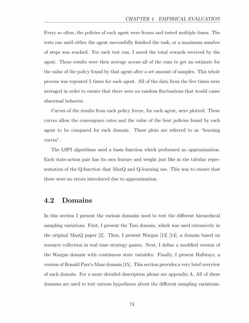
CHAPTER 4. EMPIRICAL EVALUATION
Every so often, the policies of each agent were frozen and tested multiple times. The
tests ran until either the agent successfully finished the task, or a maximum number
of steps was reached. For each test run, I saved the total rewards received by the
agent. These results were then average across all of the runs to get an estimate for
the value of the policy found by that agent after a set amount of samples. This whole
process was repeated 5 times for each agent. All of the data from the five times were
averaged in order to ensure that there were no random fluctuations that would cause
abnormal behavior.
Curves of the results from each policy freeze, for each agent, were plotted. These
curves allow the convergence rates and the value of the best policies found by each
agent to be compared for each domain. These plots are referred to as “learning
curves”.
The LSPI algorithms used a basis function which performed no approximation.
Each state-action pair has its own feature and weight just like in the tabular repre-
sentation of the Q-function that MaxQ and Q-learning use. This was to ensure that
there were no errors introduced due to approximation.
4.2 Domains
In this section I present the various domains used to test the different hierarchical
sampling variations. First, I present the Taxi domain, which was used extensively in
the original MaxQ paper [2]. Then, I present Wargus [13] [14], a domain based on
resource collection in real time strategy games. Next, I define a modified version of
the Wargus domain with continuous state variables. Finally, I present Hallways, a
version of Ronald Parr’s Maze domain [15]. This section provides a very brief overview
of each domain. For a more detailed description please see appendix A. All of these
domains are used to test various hypotheses about the different sampling variations.
74
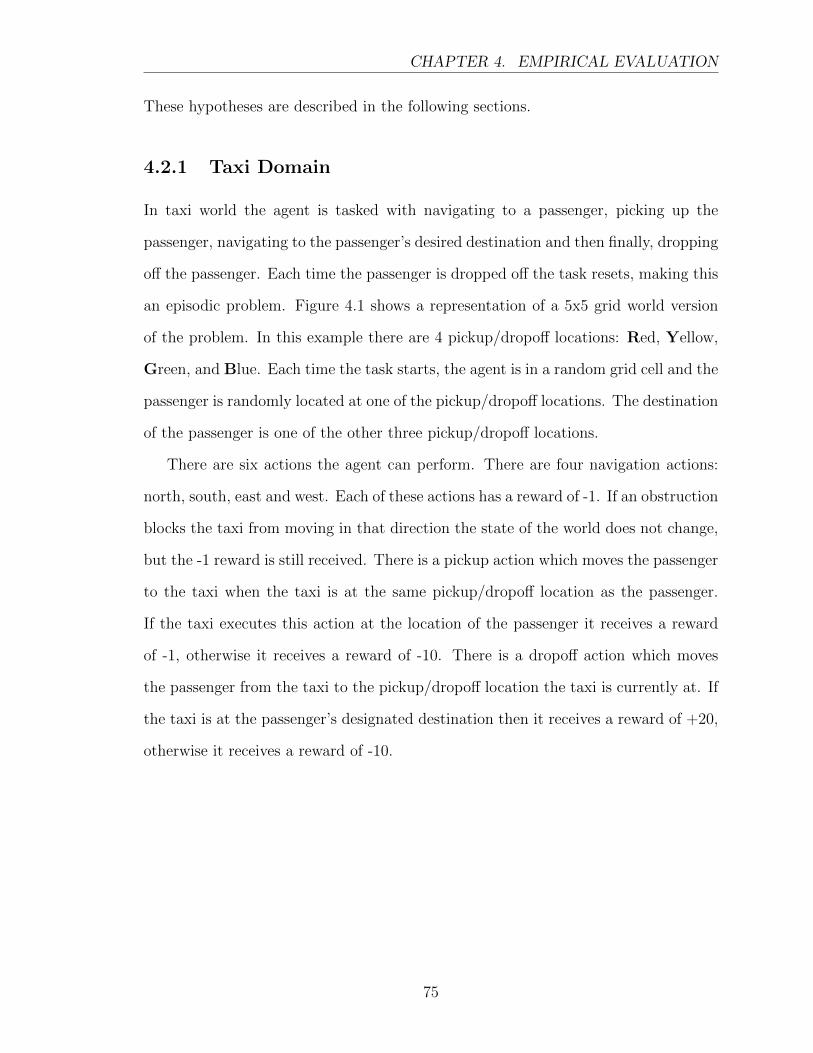
CHAPTER 4. EMPIRICAL EVALUATION
These hypotheses are described in the following sections.
4.2.1 Taxi Domain
In taxi world the agent is tasked with navigating to a passenger, picking up the
passenger, navigating to the passenger’s desired destination and then finally, dropping
off the passenger. Each time the passenger is dropped off the task resets, making this
an episodic problem. Figure 4.1 shows a representation of a 5x5 grid world version
of the problem. In this example there are 4 pickup/dropoff locations: Red, Yellow,
Green, and Blue. Each time the task starts, the agent is in a random grid cell and the
passenger is randomly located at one of the pickup/dropoff locations. The destination
of the passenger is one of the other three pickup/dropoff locations.
There are six actions the agent can perform. There are four navigation actions:
north, south, east and west. Each of these actions has a reward of -1. If an obstruction
blocks the taxi from moving in that direction the state of the world does not change,
but the -1 reward is still received. There is a pickup action which moves the passenger
to the taxi when the taxi is at the same pickup/dropoff location as the passenger.
If the taxi executes this action at the location of the passenger it receives a reward
of -1, otherwise it receives a reward of -10. There is a dropoff action which moves
the passenger from the taxi to the pickup/dropoff location the taxi is currently at. If
the taxi is at the passenger’s designated destination then it receives a reward of +20,
otherwise it receives a reward of -10.
75
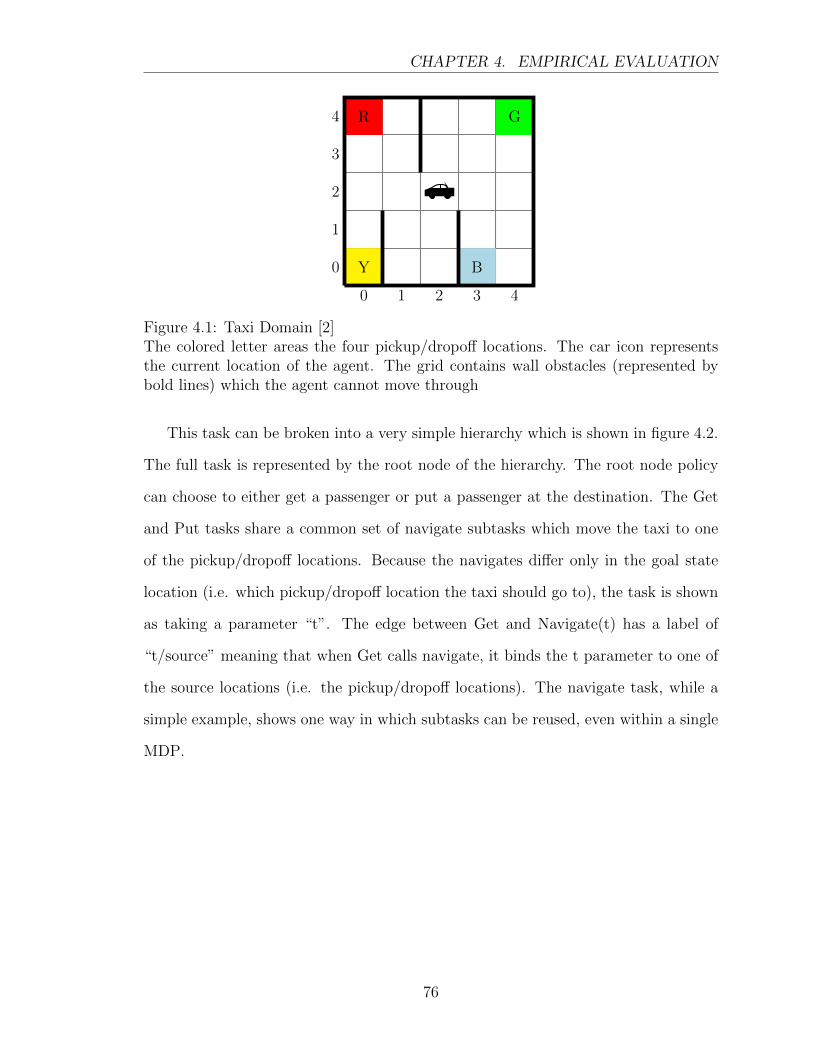
CHAPTER 4. EMPIRICAL EVALUATION
0 1 2 3 4
0
1
2
3
4 R
BY
G
Figure 4.1: Taxi Domain [2]The colored letter areas the four pickup/dropoff locations. The car icon representsthe current location of the agent. The grid contains wall obstacles (represented bybold lines) which the agent cannot move through
This task can be broken into a very simple hierarchy which is shown in figure 4.2.
The full task is represented by the root node of the hierarchy. The root node policy
can choose to either get a passenger or put a passenger at the destination. The Get
and Put tasks share a common set of navigate subtasks which move the taxi to one
of the pickup/dropoff locations. Because the navigates differ only in the goal state
location (i.e. which pickup/dropoff location the taxi should go to), the task is shown
as taking a parameter “t”. The edge between Get and Navigate(t) has a label of
“t/source” meaning that when Get calls navigate, it binds the t parameter to one of
the source locations (i.e. the pickup/dropoff locations). The navigate task, while a
simple example, shows one way in which subtasks can be reused, even within a single
MDP.
76
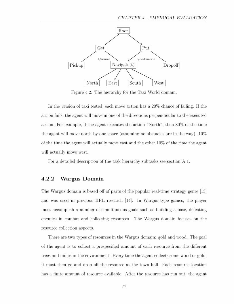
CHAPTER 4. EMPIRICAL EVALUATION
Root
Get Put
Navigate(t)Pickup Dropoff
North East South West
t/source t/destination
Figure 4.2: The hierarchy for the Taxi World domain.
In the version of taxi tested, each move action has a 20% chance of failing. If the
action fails, the agent will move in one of the directions perpendicular to the executed
action. For example, if the agent executes the action “North”, then 80% of the time
the agent will move north by one space (assuming no obstacles are in the way). 10%
of the time the agent will actually move east and the other 10% of the time the agent
will actually move west.
For a detailed description of the task hierarchy subtasks see section A.1.
4.2.2 Wargus Domain
The Wargus domain is based off of parts of the popular real-time strategy genre [13]
and was used in previous HRL research [14]. In Wargus type games, the player
must accomplish a number of simultaneous goals such as building a base, defeating
enemies in combat and collecting resources. The Wargus domain focuses on the
resource collection aspects.
There are two types of resources in the Wargus domain: gold and wood. The goal
of the agent is to collect a prespecified amount of each resource from the different
trees and mines in the environment. Every time the agent collects some wood or gold,
it must then go and drop off the resource at the town hall. Each resource location
has a finite amount of resource available. After the resource has run out, the agent
77
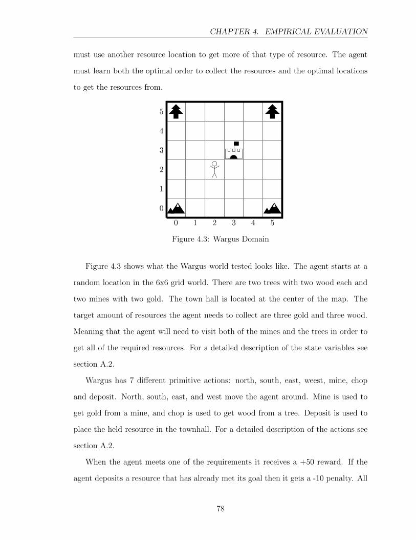
CHAPTER 4. EMPIRICAL EVALUATION
must use another resource location to get more of that type of resource. The agent
must learn both the optimal order to collect the resources and the optimal locations
to get the resources from.
0 1 2 3 4 5
0
1
2
3
4
5
Figure 4.3: Wargus Domain
Figure 4.3 shows what the Wargus world tested looks like. The agent starts at a
random location in the 6x6 grid world. There are two trees with two wood each and
two mines with two gold. The town hall is located at the center of the map. The
target amount of resources the agent needs to collect are three gold and three wood.
Meaning that the agent will need to visit both of the mines and the trees in order to
get all of the required resources. For a detailed description of the state variables see
section A.2.
Wargus has 7 different primitive actions: north, south, east, weest, mine, chop
and deposit. North, south, east, and west move the agent around. Mine is used to
get gold from a mine, and chop is used to get wood from a tree. Deposit is used to
place the held resource in the townhall. For a detailed description of the actions see
section A.2.
When the agent meets one of the requirements it receives a +50 reward. If the
agent deposits a resource that has already met its goal then it gets a -10 penalty. All
78
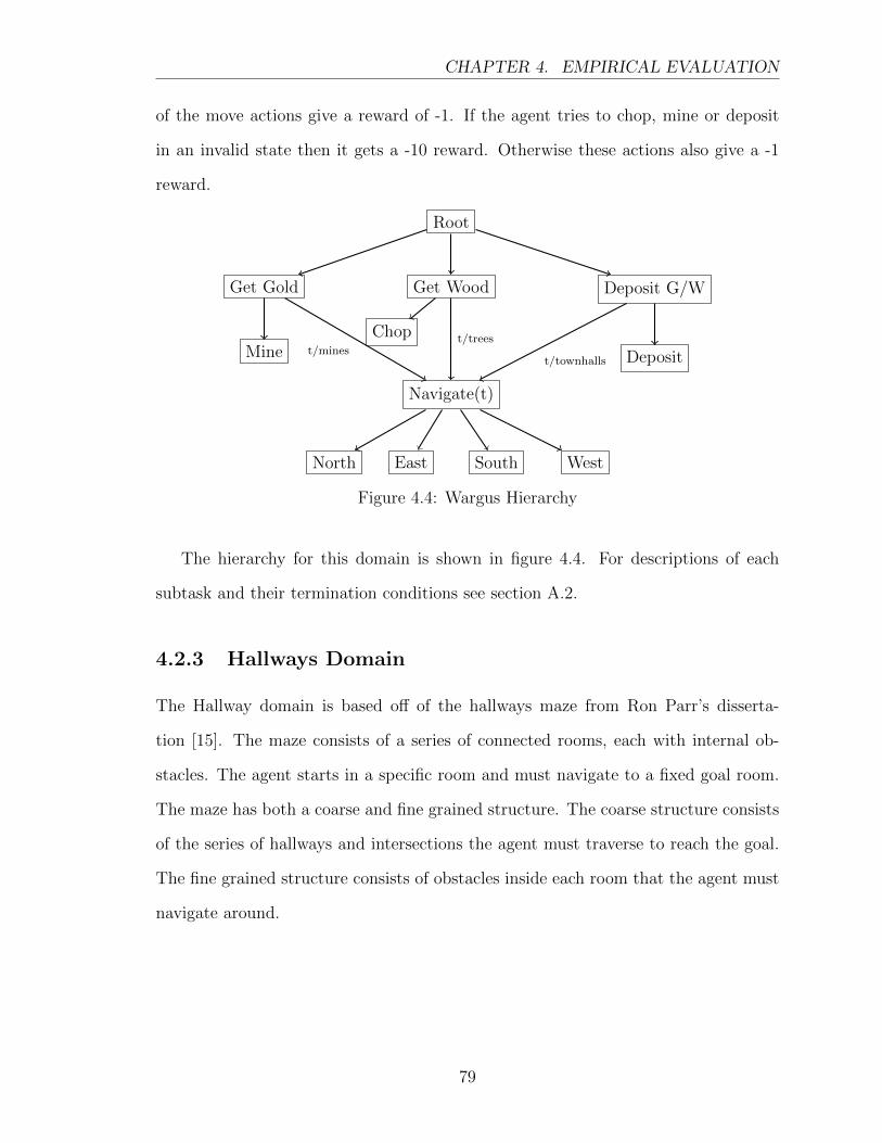
CHAPTER 4. EMPIRICAL EVALUATION
of the move actions give a reward of -1. If the agent tries to chop, mine or deposit
in an invalid state then it gets a -10 reward. Otherwise these actions also give a -1
reward.
Root
Get Gold Get Wood Deposit G/W
MineChop
Deposit
Navigate(t)
North East South West
t/minest/trees
t/townhalls
Figure 4.4: Wargus Hierarchy
The hierarchy for this domain is shown in figure 4.4. For descriptions of each
subtask and their termination conditions see section A.2.
4.2.3 Hallways Domain
The Hallway domain is based off of the hallways maze from Ron Parr’s disserta-
tion [15]. The maze consists of a series of connected rooms, each with internal ob-
stacles. The agent starts in a specific room and must navigate to a fixed goal room.
The maze has both a coarse and fine grained structure. The coarse structure consists
of the series of hallways and intersections the agent must traverse to reach the goal.
The fine grained structure consists of obstacles inside each room that the agent must
navigate around.
79
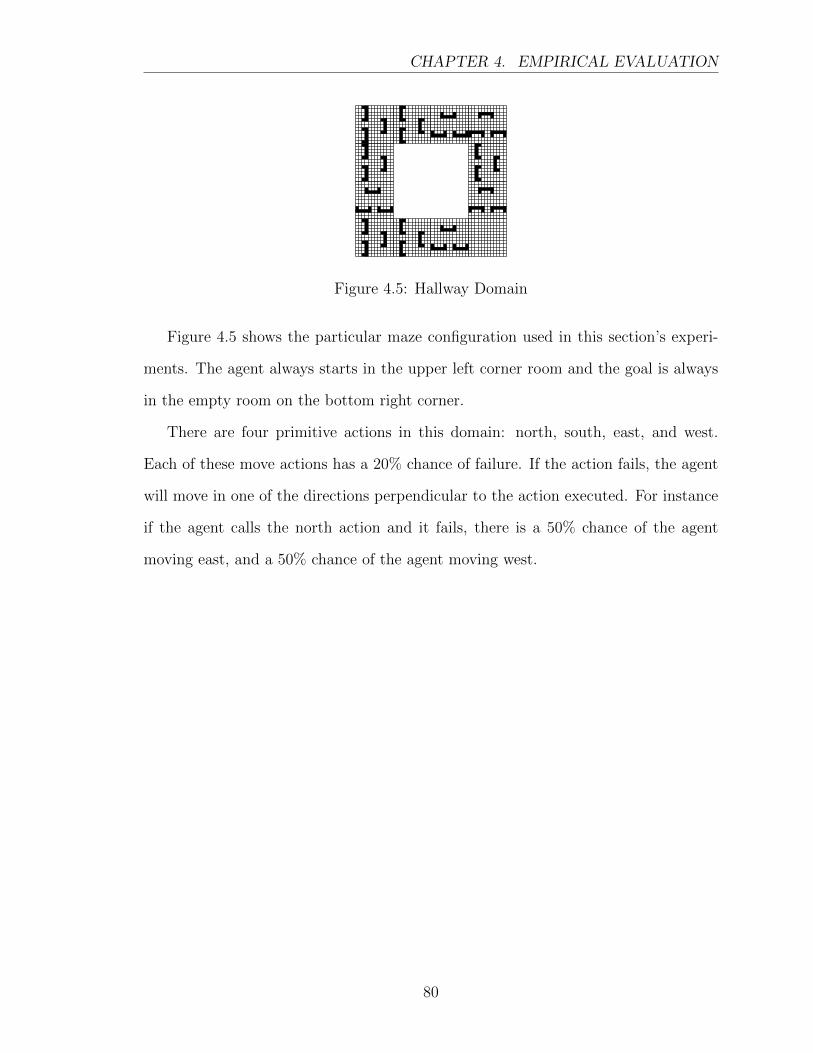
CHAPTER 4. EMPIRICAL EVALUATION
Figure 4.5: Hallway Domain
Figure 4.5 shows the particular maze configuration used in this section’s experi-
ments. The agent always starts in the upper left corner room and the goal is always
in the empty room on the bottom right corner.
There are four primitive actions in this domain: north, south, east, and west.
Each of these move actions has a 20% chance of failure. If the action fails, the agent
will move in one of the directions perpendicular to the action executed. For instance
if the agent calls the north action and it fails, there is a 50% chance of the agent
moving east, and a 50% chance of the agent moving west.
80
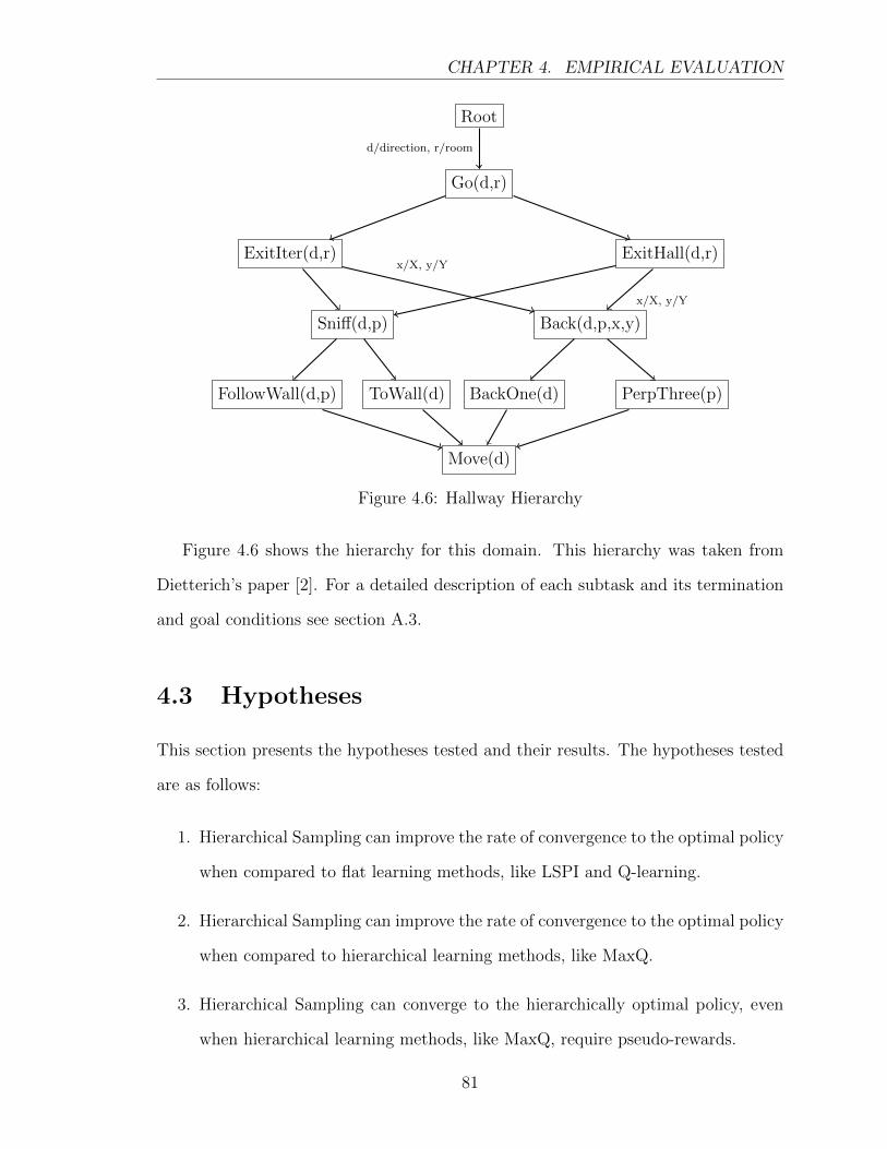
CHAPTER 4. EMPIRICAL EVALUATION
Root
Go(d,r)
ExitIter(d,r) ExitHall(d,r)
Sniff(d,p) Back(d,p,x,y)
FollowWall(d,p) ToWall(d) BackOne(d) PerpThree(p)
Move(d)
d/direction, r/room
x/X, y/Y
x/X, y/Y
Figure 4.6: Hallway Hierarchy
Figure 4.6 shows the hierarchy for this domain. This hierarchy was taken from
Dietterich’s paper [2]. For a detailed description of each subtask and its termination
and goal conditions see section A.3.
4.3 Hypotheses
This section presents the hypotheses tested and their results. The hypotheses tested
are as follows:
1. Hierarchical Sampling can improve the rate of convergence to the optimal policy
when compared to flat learning methods, like LSPI and Q-learning.
2. Hierarchical Sampling can improve the rate of convergence to the optimal policy
when compared to hierarchical learning methods, like MaxQ.
3. Hierarchical Sampling can converge to the hierarchically optimal policy, even
when hierarchical learning methods, like MaxQ, require pseudo-rewards.
81
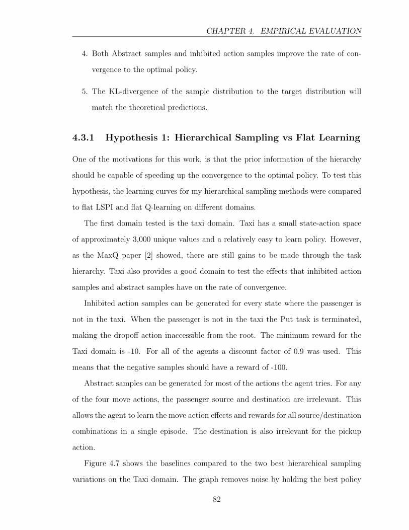
CHAPTER 4. EMPIRICAL EVALUATION
4. Both Abstract samples and inhibited action samples improve the rate of con-
vergence to the optimal policy.
5. The KL-divergence of the sample distribution to the target distribution will
match the theoretical predictions.
4.3.1 Hypothesis 1: Hierarchical Sampling vs Flat Learning
One of the motivations for this work, is that the prior information of the hierarchy
should be capable of speeding up the convergence to the optimal policy. To test this
hypothesis, the learning curves for my hierarchical sampling methods were compared
to flat LSPI and flat Q-learning on different domains.
The first domain tested is the taxi domain. Taxi has a small state-action space
of approximately 3,000 unique values and a relatively easy to learn policy. However,
as the MaxQ paper [2] showed, there are still gains to be made through the task
hierarchy. Taxi also provides a good domain to test the effects that inhibited action
samples and abstract samples have on the rate of convergence.
Inhibited action samples can be generated for every state where the passenger is
not in the taxi. When the passenger is not in the taxi the Put task is terminated,
making the dropoff action inaccessible from the root. The minimum reward for the
Taxi domain is -10. For all of the agents a discount factor of 0.9 was used. This
means that the negative samples should have a reward of -100.
Abstract samples can be generated for most of the actions the agent tries. For any
of the four move actions, the passenger source and destination are irrelevant. This
allows the agent to learn the move action effects and rewards for all source/destination
combinations in a single episode. The destination is also irrelevant for the pickup
action.
Figure 4.7 shows the baselines compared to the two best hierarchical sampling
variations on the Taxi domain. The graph removes noise by holding the best policy
82
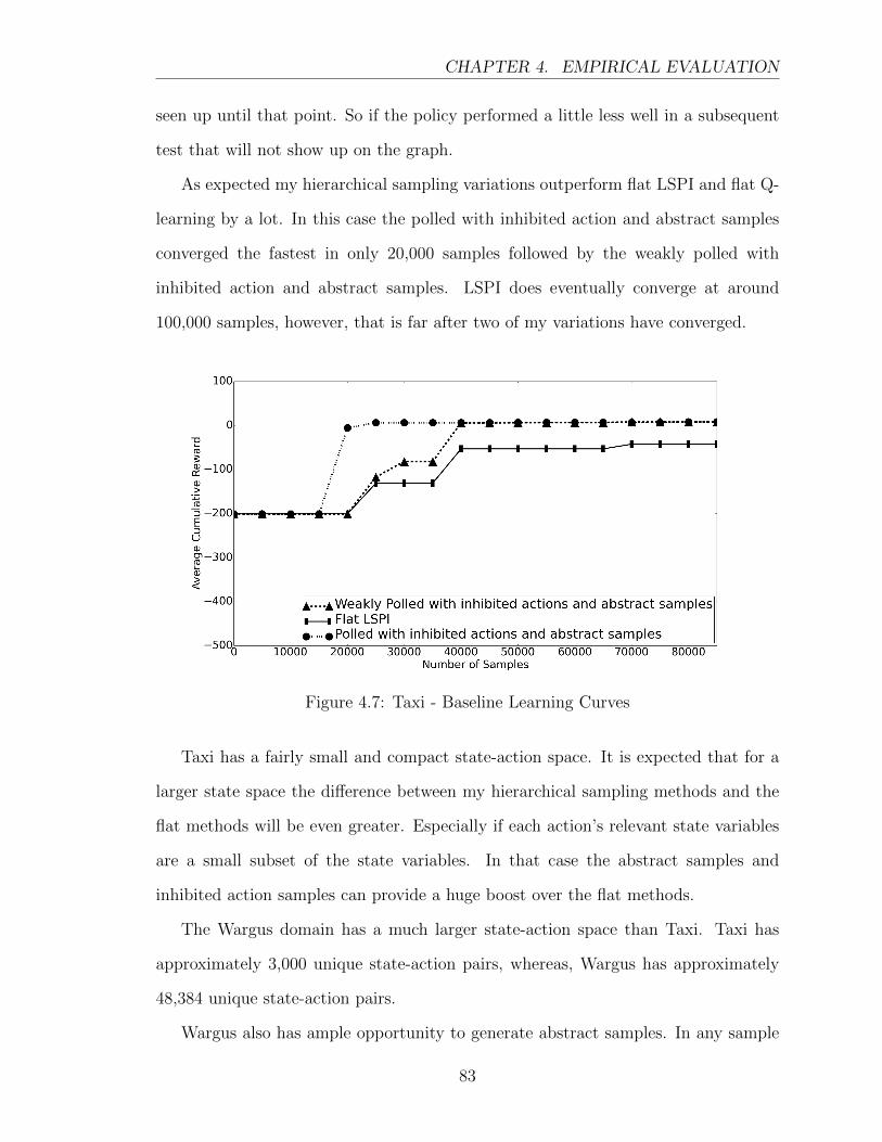
CHAPTER 4. EMPIRICAL EVALUATION
seen up until that point. So if the policy performed a little less well in a subsequent
test that will not show up on the graph.
As expected my hierarchical sampling variations outperform flat LSPI and flat Q-
learning by a lot. In this case the polled with inhibited action and abstract samples
converged the fastest in only 20,000 samples followed by the weakly polled with
inhibited action and abstract samples. LSPI does eventually converge at around
100,000 samples, however, that is far after two of my variations have converged.
Figure 4.7: Taxi - Baseline Learning Curves
Taxi has a fairly small and compact state-action space. It is expected that for a
larger state space the difference between my hierarchical sampling methods and the
flat methods will be even greater. Especially if each action’s relevant state variables
are a small subset of the state variables. In that case the abstract samples and
inhibited action samples can provide a huge boost over the flat methods.
The Wargus domain has a much larger state-action space than Taxi. Taxi has
approximately 3,000 unique state-action pairs, whereas, Wargus has approximately
48,384 unique state-action pairs.
Wargus also has ample opportunity to generate abstract samples. In any sample
83
CHAPTER 4. EMPIRICAL EVALUATION
for a move action (North, South, East, West) only the X and Y location variables
are relevant. When mining, the variables related to the wood collection portion of
the task are irrelevant. Similarly when the agent is chopping wood, the variables
related to the gold collection portion of the task are irrelevant. The flat methods
need to manually collect samples in order to learn which states are irrelevant for a
given action, but the hierarchical methods can generate them through the abstract
sample procedure.
Inhibited action samples are also useful in Wargus. When the agent is not holding
any resource, the deposit action is unavailable. The inhibited action samples should
quickly teach the agent not to call deposit when it has no resource. The environment
also provides a negative reward for calling deposit in these states, meaning the flat
learning methods will eventually learn this fact. However, by using inhibited samples,
the agent does not need to waste time collecting samples for these actions. Similarly,
inhibited action samples can be generated for chop and mine when the agent has a
resource or that particular resource’s goal has been met.
Figure 4.8 shows the baselines compared to the top three hierarchical sampling
variations on the Wargus domain. Again the best policies were held across points.
As expected my hierarchical sampling methods do significantly better than the flat
learning algorithms. All three variations converge within 20,000 samples to the opti-
mal policy, compared to flat LSPI which even by 100,000 samples has not yet found
the optimal policy.
84
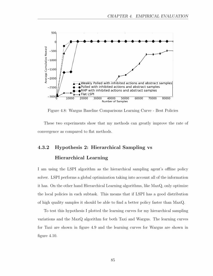
CHAPTER 4. EMPIRICAL EVALUATION
Figure 4.8: Wargus Baseline Comparisons Learning Curve - Best Policies
These two experiments show that my methods can greatly improve the rate of
convergence as compared to flat methods.
4.3.2 Hypothesis 2: Hierarchical Sampling vs
Hierarchical Learning
I am using the LSPI algorithm as the hierarchical sampling agent’s offline policy
solver. LSPI performs a global optimization taking into account all of the information
it has. On the other hand Hierarchical Learning algorithms, like MaxQ, only optimize
the local policies in each subtask. This means that if LSPI has a good distribution
of high quality samples it should be able to find a better policy faster than MaxQ.
To test this hypothesis I plotted the learning curves for my hierarchical sampling
variations and the MaxQ algorithm for both Taxi and Wargus. The learning curves
for Taxi are shown in figure 4.9 and the learning curves for Wargus are shown in
figure 4.10.
85
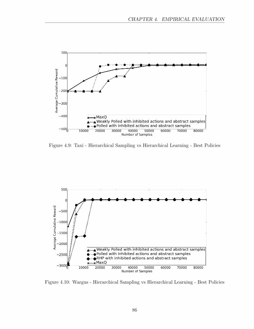
CHAPTER 4. EMPIRICAL EVALUATION
Figure 4.9: Taxi - Hierarchical Sampling vs Hierarchical Learning - Best Policies
Figure 4.10: Wargus - Hierarchical Sampling vs Hierarchical Learning - Best Policies
86
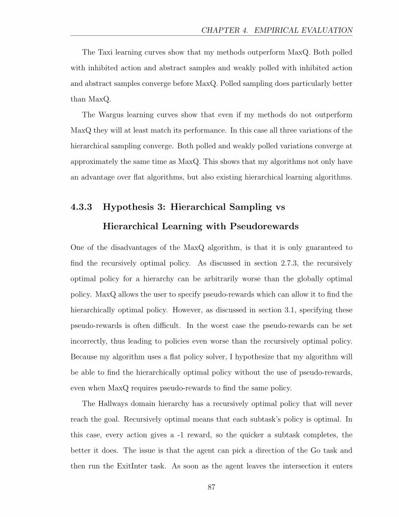
CHAPTER 4. EMPIRICAL EVALUATION
The Taxi learning curves show that my methods outperform MaxQ. Both polled
with inhibited action and abstract samples and weakly polled with inhibited action
and abstract samples converge before MaxQ. Polled sampling does particularly better
than MaxQ.
The Wargus learning curves show that even if my methods do not outperform
MaxQ they will at least match its performance. In this case all three variations of the
hierarchical sampling converge. Both polled and weakly polled variations converge at
approximately the same time as MaxQ. This shows that my algorithms not only have
an advantage over flat algorithms, but also existing hierarchical learning algorithms.
4.3.3 Hypothesis 3: Hierarchical Sampling vs
Hierarchical Learning with Pseudorewards
One of the disadvantages of the MaxQ algorithm, is that it is only guaranteed to
find the recursively optimal policy. As discussed in section 2.7.3, the recursively
optimal policy for a hierarchy can be arbitrarily worse than the globally optimal
policy. MaxQ allows the user to specify pseudo-rewards which can allow it to find the
hierarchically optimal policy. However, as discussed in section 3.1, specifying these
pseudo-rewards is often difficult. In the worst case the pseudo-rewards can be set
incorrectly, thus leading to policies even worse than the recursively optimal policy.
Because my algorithm uses a flat policy solver, I hypothesize that my algorithm will
be able to find the hierarchically optimal policy without the use of pseudo-rewards,
even when MaxQ requires pseudo-rewards to find the same policy.
The Hallways domain hierarchy has a recursively optimal policy that will never
reach the goal. Recursively optimal means that each subtask’s policy is optimal. In
this case, every action gives a -1 reward, so the quicker a subtask completes, the
better it does. The issue is that the agent can pick a direction of the Go task and
then run the ExitInter task. As soon as the agent leaves the intersection it enters
87
CHAPTER 4. EMPIRICAL EVALUATION
the ExitHall subtask. If the agent calls the Back subtask, then it will reenter the
intersection, causing Back and ExitHall to terminate in a single step. The agent will
then call ExitInter again and keep repeating this sequence forever. This is because
the number of steps to actually exit the hallway in the correct direction will be a lot
more than the one step it takes for the agent to just go back into the intersection it
just left. Hence, without pseudo-rewards MaxQ will perform terribly on this domain.
Pseudo-rewards are necessary for MaxQ to find a policy that at least reaches the
goal. I define the pseudo-rewards as +1000 if the ExitHall subtask exits into the
goal intersection and -1000 if the ExitHall subtask exits into any other intersection,
including the one it just came from. So if the agent calls ExitHall(north, room8) and
it successfully enters the intersection north of room8, it will receive a pseudo-reward
of +1000. If it instead enters the intersection in room8, it will receive a pseudo-
reward of -1000. Even if the agent takes a very circuitous route through the obstacles
it will take far less than 1000 steps for it to reach the goal intersection. So now
internally ExitHall will consider the sniff actions as a better choice than the back
action. It is important to note that I cannot prove that these pseudo-rewards are the
best pseudo-rewards possible, however, as will be shown they do improve the policy
MaxQ finds.
While MaxQ with pseudo-rewards can converge to the hierarchically optimal pol-
icy for Hallways, the hierarchically optimal policy will not be as good as a globally
optimal policy that can be found by algorithms such as flat Q-learning and flat LSPI.
Given the Hallways hierarchy, the MaxQ agent is stuck moving forward until it hits
an obstacle. Before it can get out of the obstacle and go around, it first has to slide
along the obstacle until it hits a corner. On the other hand, the flat policies can
preemptively move around the obstacle. Also the hierarchical policy has to pick a
sliding direction and stick with it until it either finishes the subtask or gets stuck.
If noise causes the agent to drift then it might be more optimal to pick a different
88
CHAPTER 4. EMPIRICAL EVALUATION
perpendicular direction to slide in. These two effects cause the globally optimal pol-
icy found by the flat methods to perform better than the hierarchical optimal policy
found by algorithms like MaxQ.
Unlike in the Taxi and Wargus domains, Hallways has no irrelevant state variables,
so no abstract samples can be generated. However, inhibited actions can be generated
for move actions that would attempt to move the agent into a wall or obstacle.
In the general case I expect my algorithm will only be able to converge to the
hierarchically optimal policy, however, Hallways is a special case where hierarchical
sampling can find the globally optimal policy. In Hallways the hierarchy is such
that the hierarchical sampling agent will receive samples for every action in every
state. These samples will either come from directly sampling the environment or
from deriving inhibited samples. Because LSPI will receive samples for every state-
action pair, LSPI should be able to find the globally optimal policy. In the general
case only hierarchically optimal policies can be guaranteed because the hierarchy may
stop state-action pairs that are important to the globally optimal policy from being
sampled. If such a hierarchy was used for sampling, then policy solver would be
missing the information it needs to find the globally optimal policy.
Figure 4.11 shows the learning curves of the best hierarchical sampling variations
and MaxQ with pseudo-rewards.
89
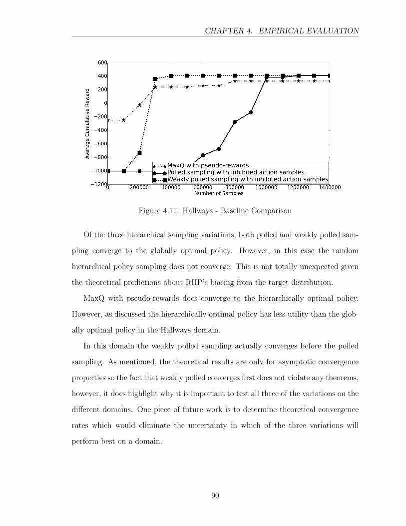
CHAPTER 4. EMPIRICAL EVALUATION
Figure 4.11: Hallways - Baseline Comparison
Of the three hierarchical sampling variations, both polled and weakly polled sam-
pling converge to the globally optimal policy. However, in this case the random
hierarchical policy sampling does not converge. This is not totally unexpected given
the theoretical predictions about RHP’s biasing from the target distribution.
MaxQ with pseudo-rewards does converge to the hierarchically optimal policy.
However, as discussed the hierarchically optimal policy has less utility than the glob-
ally optimal policy in the Hallways domain.
In this domain the weakly polled sampling actually converges before the polled
sampling. As mentioned, the theoretical results are only for asymptotic convergence
properties so the fact that weakly polled converges first does not violate any theorems,
however, it does highlight why it is important to test all three of the variations on the
different domains. One piece of future work is to determine theoretical convergence
rates which would eliminate the uncertainty in which of the three variations will
perform best on a domain.
90
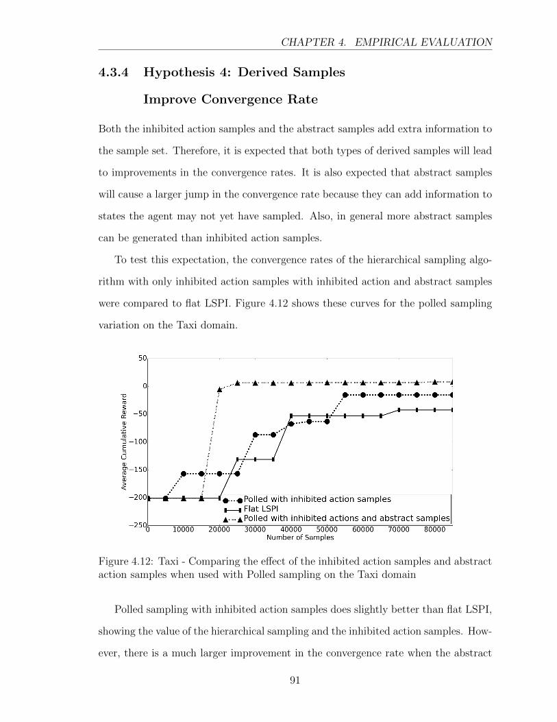
CHAPTER 4. EMPIRICAL EVALUATION
4.3.4 Hypothesis 4: Derived Samples
Improve Convergence Rate
Both the inhibited action samples and the abstract samples add extra information to
the sample set. Therefore, it is expected that both types of derived samples will lead
to improvements in the convergence rates. It is also expected that abstract samples
will cause a larger jump in the convergence rate because they can add information to
states the agent may not yet have sampled. Also, in general more abstract samples
can be generated than inhibited action samples.
To test this expectation, the convergence rates of the hierarchical sampling algo-
rithm with only inhibited action samples with inhibited action and abstract samples
were compared to flat LSPI. Figure 4.12 shows these curves for the polled sampling
variation on the Taxi domain.
Figure 4.12: Taxi - Comparing the effect of the inhibited action samples and abstractaction samples when used with Polled sampling on the Taxi domain
Polled sampling with inhibited action samples does slightly better than flat LSPI,
showing the value of the hierarchical sampling and the inhibited action samples. How-
ever, there is a much larger improvement in the convergence rate when the abstract
91
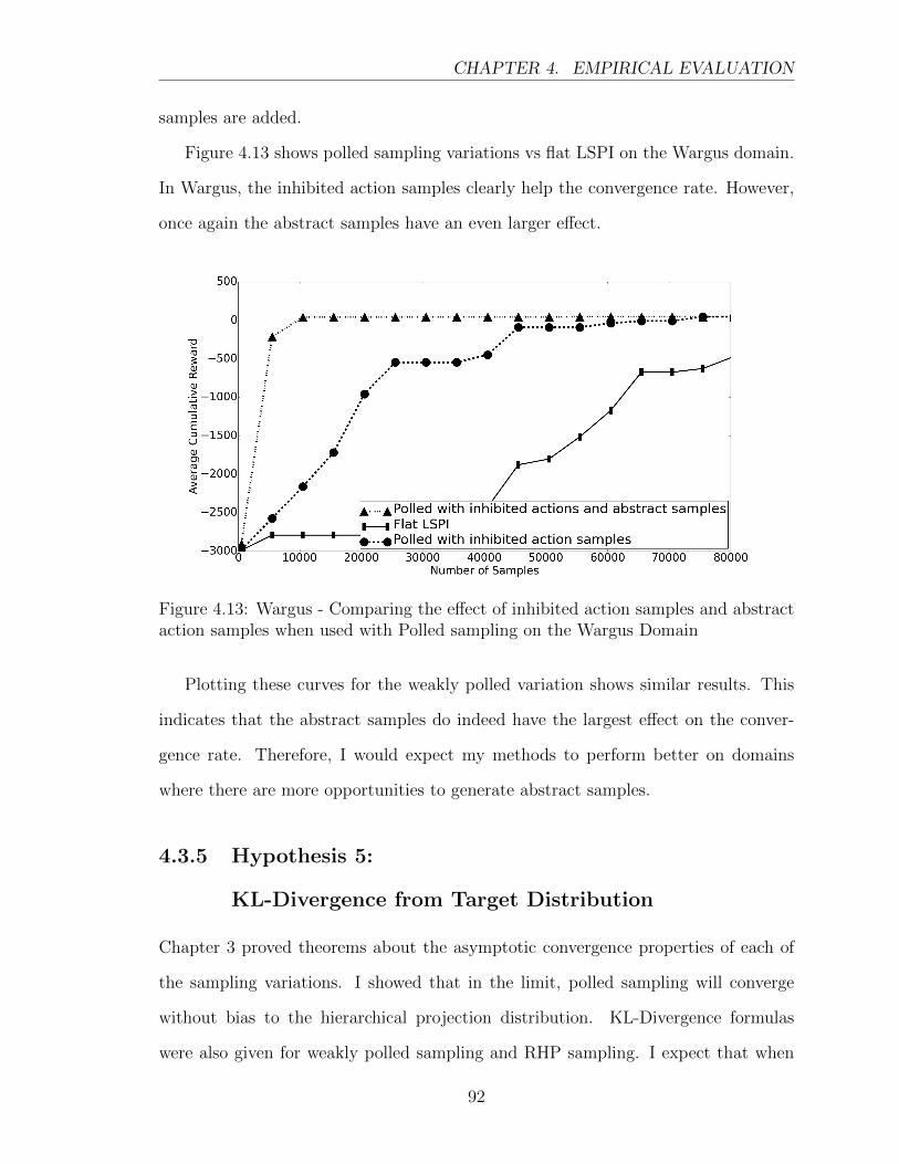
CHAPTER 4. EMPIRICAL EVALUATION
samples are added.
Figure 4.13 shows polled sampling variations vs flat LSPI on the Wargus domain.
In Wargus, the inhibited action samples clearly help the convergence rate. However,
once again the abstract samples have an even larger effect.
Figure 4.13: Wargus - Comparing the effect of inhibited action samples and abstractaction samples when used with Polled sampling on the Wargus Domain
Plotting these curves for the weakly polled variation shows similar results. This
indicates that the abstract samples do indeed have the largest effect on the conver-
gence rate. Therefore, I would expect my methods to perform better on domains
where there are more opportunities to generate abstract samples.
4.3.5 Hypothesis 5:
KL-Divergence from Target Distribution
Chapter 3 proved theorems about the asymptotic convergence properties of each of
the sampling variations. I showed that in the limit, polled sampling will converge
without bias to the hierarchical projection distribution. KL-Divergence formulas
were also given for weakly polled sampling and RHP sampling. I expect that when
92
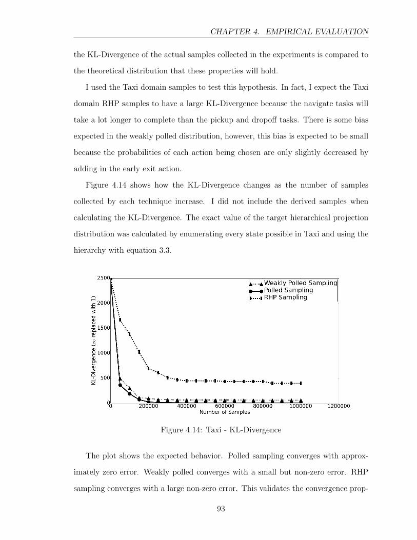
CHAPTER 4. EMPIRICAL EVALUATION
the KL-Divergence of the actual samples collected in the experiments is compared to
the theoretical distribution that these properties will hold.
I used the Taxi domain samples to test this hypothesis. In fact, I expect the Taxi
domain RHP samples to have a large KL-Divergence because the navigate tasks will
take a lot longer to complete than the pickup and dropoff tasks. There is some bias
expected in the weakly polled distribution, however, this bias is expected to be small
because the probabilities of each action being chosen are only slightly decreased by
adding in the early exit action.
Figure 4.14 shows how the KL-Divergence changes as the number of samples
collected by each technique increase. I did not include the derived samples when
calculating the KL-Divergence. The exact value of the target hierarchical projection
distribution was calculated by enumerating every state possible in Taxi and using the
hierarchy with equation 3.3.
Figure 4.14: Taxi - KL-Divergence
The plot shows the expected behavior. Polled sampling converges with approx-
imately zero error. Weakly polled converges with a small but non-zero error. RHP
sampling converges with a large non-zero error. This validates the convergence prop-
93

CHAPTER 4. EMPIRICAL EVALUATION
erties analyzed in chapter 3.
94

Chapter 5
Conclusions
In this work, I have introduced a new sampling algorithm that uses prior informa-
tion encoded in a task hierarchy, to direct sample collection for an offline learning
algorithm. While this idea can be applied to other offline algorithms and other task
hierarchy frameworks, I have focused my analysis and experiments on the use of LSPI
and the MaxQ framework. I introduced the target distribution that a hierarchical
sampling algorithm should converge to through the new “hierarchical projection” op-
eration. I then used this distribution to analyze three different variations on the basic
hierarchical sampling algorithm in the process proving properties of their asymptotic
convergence to the target distribution. I also introduced the concept of “derived
samples”, which allow an agent to expand the samples it has collected using addi-
tional information encoded in a task hierarchy. Through multiple experiments I have
shown that my hierarchical sampling algorithm not only outperforms flat learning
algorithms, such as Q-learning and LSPI, but that it can also outperform hierarchical
learning algorithms, such as MaxQ. I have also shown that for domains which MaxQ
requires pseudo-rewards to converge, my algorithm is capable of finding the hier-
archically optimal policy with no pseudo-rewards. Additionally, I have shown that
derived samples can significantly improve the rate of convergence to the optimal pol-
95
CHAPTER 5. CONCLUSIONS
icy. Finally, I have experimentally validated the theoretical asymptotic convergence
properties for the hierarchical sampling variations.
The main limitation of the hierarchical sampling technique is the amount of com-
putational resources needed to find the policy. LSPI does a global optimization by
solving a large set of linear equations. This optimization can take a long time and
use a lot of memory. Therefore, it would be useful to investigate methods of reduc-
ing these computational costs, such as by verifying that approximation works with
my algorithm. This thesis also does not provide theoretical analysis of the rate of
convergence. So future work should examine theoretical convergence rates. Finally,
a stronger theoretical basis should be developed for the derived samples.
This work provides a theoretical framework to analyze any future hierarchical
sampling results. More importantly, this work has proven that when compared to
existing methods, using the task hierarchy to direct sample collection can have large
positive effects, both on the rate of policy convergence, and the quality of the con-
verged policies.
96
Bibliography
[1] M. G. Lagoudakis and R. Parr, “Least-Squares Policy Iteration,” pp. 1107–1149,
2003. [Online]. Available: https://www.cs.duke.edu/research/AI/LSPI/jmlr03.
[2] T. G. Dietterich, “Hierarchical Reinforcement Learning with MAXQ Value
Function Decomposition,” J. Artif. Intell. Res.(JAIR), vol. 13, pp. 227–303, 2000.
[Online]. Available: http://www.jair.org/media/639/live-639-1834-jair.pdf
[3] M. L. Puterman, Markov Decision Processes: Discrete Stochastic Dynamic Pro-
gramming. Hoboken, NJ USA: John Wiley & Sons, Inc., 2005.
[4] L. P. Kaelbling, M. L. Littman, and A. W. Moore, “Reinforcement learning: A
survey,” Journal of artificial intelligence research, pp. 237–285, 1996.
[5] R. Bellman, “Dynamic programming and Lagrange multipliers,” Proceedings of
the National Academy of Sciences of the United States of America, vol. 42, no. 10,
p. 767, 1956.
[6] R. S. Sutton, H. R. Maei, and C. Szepesvari, “A convergent o(n)
temporal-difference algorithm for off-policy learning with linear function
approximation,” in Advances in Neural Information Processing Systems 21,
D. Koller, D. Schuurmans, Y. Bengio, and L. Bottou, Eds. Curran Associates,
Inc., 2009, pp. 1609–1616. [Online]. Available: http://papers.nips.cc/paper/
97
BIBLIOGRAPHY
3626-a-convergent-on-temporal-difference-algorithm-for-off-policy-learning-with-linear-function-approximation.
[7] F. Cao and S. Ray, “Bayesian Hierarchical Reinforcement Learning,” in Advances
in Neural Information Processing Systems, 2012, pp. 73–81. [Online]. Available:
http://papers.nips.cc/paper/4752-bayesian-hierarchical-reinforcement-learning
[8] R. Parr and S. Russell, “Reinforcement learning with hierarchies of machines,”
pp. 1043–1049, Jul. 1998. [Online]. Available: http://dl.acm.org/citation.cfm?
id=302528.302894
[9] R. S. Sutton, D. Precup, and S. Singh, “Between MDPs and semi-MDPs: A
framework for temporal abstraction in reinforcement learning,” Artificial intelli-
gence, vol. 112, no. 1, pp. 181–211, 1999.
[10] D. Andre and S. J. Russell, “State abstraction for programmable reinforcement
learning agents,” in AAAI/IAAI, 2002, pp. 119–125.
[11] L. Lovasz, “Random Walks on Graphs: A Survey,” pp. 1–46, 1993. [Online].
Available: http://www.cs.elte.hu/∼lovasz/erdos.pdf
[12] D. Aldous and J. A. Fill, “Reversible Markov Chains and Random Walks on
Graphs,” vol. 2002, 2014.
[13] Pali and Stratagus Team, “Wargus,” 2010. [Online]. Available: https:
//launchpad.net/wargus
[14] N. Mehta, S. Ray, P. Tadepalli, and T. Dietterich, “Automatic discovery and
transfer of MAXQ hierarchies,” in Proceedings of the 25th international confer-
ence on Machine learning. ACM, 2008, pp. 648–655.
[15] R. E. Parr, “Hierarchical control and learning for Markov decision processes,”
Ph.D. dissertation, Citeseer, 1998.
98
BIBLIOGRAPHY
[16] R. S. Sutton and A. G. Barto, Reinforcement learning: An introduction. MIT
press Cambridge, 1998, vol. 1, no. 1.
[17] C. J. C. H. Watkins and P. Dayan, “Q-learning,” Machine Learning,
vol. 8, no. 3-4, pp. 279–292, May 1992. [Online]. Available: http:
//link.springer.com/10.1007/BF00992698
[18] M. Wiering and M. van Otterlo, Reinforcement Learning State-of-the-Art, M.-H.
Lim, Y.-S. Ong, M. Wiering, and M. van Otterlo, Eds. Berlin, Heidelberg:
Springer-Verlag, 2012.
[19] A. Bai, F. Wu, and X. Chen, “Online planning for large MDPs with MAXQ
decomposition,” in Proceedings of the 11th International Conference on Au-
tonomous Agents and Multiagent Systems-Volume 3. International Foundation
for Autonomous Agents and Multiagent Systems, 2012, pp. 1215–1216.
[20] S. Roncagliolo and P. Tadepalli, “Function approximation in hierarchical rela-
tional reinforcement learning,” in Proceedings of the ICML-2004 Workshop on
Relational Reinforcement Learning, 2004, pp. 1–5.
[21] K. Grave and S. Behnke, “Bayesian exploration and interactive demonstration
in continuous state MAXQ-learning,” in Robotics and Automation (ICRA), 2014
IEEE International Conference on. IEEE, 2014, pp. 3323–3330.
99
Detailed Domain Descriptions
This appendix contains more detailed information about the different domains. This
includes a domains state variables, detailed action behaviors, and detailed subtask
descriptions.
A.1 Taxi Domain
The basic taxi description is located in section 4.2.1. Figure 4.1 gives an illustration
of the domain and figure 4.2 gives the task hierarchy.
A.1.1 Taxi State Variables
Taxi has four state variables. They are as follows:
X The X location of the grid cell the agent is currently in.
Y The Y location of the grid cell the agent is currently in.
Source When the passenger has not been picked up this represents the location the
taxi should pick the passenger up from. After the passenger has been picked up
it represents whether the passenger is still in the taxi or whether the passenger
has been dropped off at the destination.
Destination One of the four pickup/dropoff locations. This is the location that the
passenger should be dropped off in.
100
APPENDIX . DETAILED DOMAIN DESCRIPTIONS
A.1.2 Taxi Action Effects
The taxi actions and their effects and rewards are as follows:
North Moves the taxi up one cell unless it at the top of the grid. This action always
give a -1 reward.
East Moves the taxi right one cell unless there is a wall to the agent’s right or the
agent is in the last column. This action always give a -1 reward.
South Moves the taxi down one cell unless it is in the bottom row. This action
always give a -1 reward.
West Moves the taxi left one cell unless there is a wall to the agent’s left or the agent
is in the first column. This action always give a -1 reward.
Pickup If the taxi is at the passenger’s source location then this moves the passenger
into the taxi and give a -1 reward. Otherwise nothing happens and the agent
gets a -10 reward.
Dropoff If the passenger is in the taxi and the taxi is at the correct dropoff loca-
tion then this moves the passenger to the destination and give a +20 reward.
Otherwise nothing happens and the agent gets a -10 reward
A.1.3 Taxi Subtask Descriptions
The termination conditions for each subtask are as follows:
Root This is the original MDP. The goal is to dropoff the passenger at the specified
dropoff location.
Get The goal of this subtask is to navigate to and pickup the passenger. This subtask
is only executable if the passenger is not currently in the taxi.
101
APPENDIX . DETAILED DOMAIN DESCRIPTIONS
Put The goal of this subtask is to navigate to the destination and dropoff the pas-
senger. This subtask is only executable if the passenger is in the taxi.
Pickup This is the primitive pickup action. If the taxi is at the location of the
passenger it succeeds.
Dropoff This is the primitive dropoff action. if the taxi is at the destination of the
passenger and the passenger is in the taxi then this succeeds.
Navigate(t) The goal is for the agent to navigate to the location specified by the “t”
parameter. When called from Get t is bound to one of the 4 source locations.
When called from Put t is bound to one of the 4 destination locations. This
subtask is terminated when the taxi is at the specified destination.
North This is the primitive move north action.
East This is the primitive move east action.
South This is the primitive move south action.
West This is the primitive move west action.
A.2 Wargus Domain
The basic Wargus description is located in section 4.2.2. Figure 4.3 shows an illus-
tration of this domain and figure 4.4 gives the hierarchy.
A.2.1 Wargus State Variables
The Wargus state variables are as follows:
X The X location of the agent in the grid world.
Y The Y location of the agent in the grid world.
102

APPENDIX . DETAILED DOMAIN DESCRIPTIONS
Resource The resource held by the agent. It has three values: None, Gold and
Wood.
Tree 1 Has Wood 1 if the tree at (0, 5) still has wood, 0 otherwise.
Tree 2 Has Wood 1 if the tree at (5, 5) still has wood, 0 otherwise.
Mine 1 Has Gold 1 if the mine at (0, 0) still has gold, 0 otherwise.
Mine 2 Has Gold 1 if the mine at (5, 0) still has gold, 0 otherwise.
Wood Requirement Met 1 if the agent has collected the goal amount of wood, 0
otherwise.
Gold Requirement Met 1 if the agent has collected the goal amount of gold, 0
otherwise.
A.2.2 Wargus Action Effects
The Wargus actions are as follows:
North Move the agent up one cell in the grid
East Move the agent one cell right in the grid
South Move the agent one cell down in the grid
West Move the agent one cell left in the grid
Mine Gold If the agent is on the location of a gold mine and that gold mine has
gold, and the agent is holding nothing, then change the resource held by the
agent to “Gold”.
Chop Wood If the agent is next to the location of a tree and that tree has wood,
and the agent is hold nothing, then change the resource held by the agent to
“Wood”
103
APPENDIX . DETAILED DOMAIN DESCRIPTIONS
Deposit If the agent is hold either gold or wood, and is next to the town hall, then
change the resource held by the agent to “None” and increase the resource count
for that resource. If the resource count matches the goal amount of resources
then change the appropriate requirement met variable to 1.
A.2.3 Wargus Subtask Descriptions
The termination conditions for each subtask are as follows:
Root This task is terminated when both “Wood Requirement Met” and “Gold Re-
quirement Met” are 1.
Get Gold This task is terminated when the agent is holding either gold or wood. It
is also terminated when the “Gold Requirement Met” variable is 1.
Get Wood This task is terminated when the agent is holding either gold or wood.
It is also terminated when the “Wood Requirement Met” variable is 1.
Deposit GW This Task is terminated when the agent is holding nothing.
Mine This is the primitive action “Mine Gold”.
Chop This is the primitive action “Chop Wood”.
Deposit This is the primitive action “Deposit”.
Navigate(t) This task is terminated when the agent is at the location specified by
t. The “Get Gold” task binds t to the locations of the gold mines. The “Get
Wood” task binds t to the locations the agent can chop wood. The “Deposit
GW” task binds t to the locations the agent can deposit.
North This is the primitive action “North”
East This is the primitive action “East”
104
APPENDIX . DETAILED DOMAIN DESCRIPTIONS
South This is the primitive action “South”
West This is the primitive action “West”
A.3 Hallways Domain
The basic hallways domain was presented in section 4.2.3. Figure 4.5 shows an illus-
tration of the configuration used and figure 4.6 shows the task hierarchy.
A.3.1 Hallways State Variables
The state variables of Hallways are as follows:
Room The current room number of the agent.
X The X location in the current room.
Y The Y location in the current room.
A.3.2 Hallways Subtask Descriptions
The Hallways hierarchy is intended to be a close conversion of the Hierarchy of Ab-
stract Machines (HAM) that was used in Parr’s original dissertation. However, HAM
subtasks, unlike MaxQ subtasks, can have internal states. To get around this lim-
itation, separate subtasks for each internal state of the HAM are created. HAMs
can also terminate after a set amount of actions, however, MaxQ subtasks can only
terminate based on a change in the state of the subtask. Hence the large number of
subtasks and the large number of parameters when compared to the hierarchies for
wargus and taxi.
The subtasks are described as follows:
Root The original MDP task. It chooses a direction, d, to Go.
105
APPENDIX . DETAILED DOMAIN DESCRIPTIONS
Go(d,r) The parameter r is bound to the ID of the room this task is started in.
This task terminates when the agent enters an intersection other than r. If the
intersection entered is the first intersection in direction d then Go reaches a goal
termination state, otherwise it is non-goal termination state.
ExitInter(d,r) Terminates when the agent has exited room r. The termination is a
goal terminal if the agent exited in direction d.
ExitHall(d,r) Terminates when the agent has exited the current hall (i.e. entered
an intersection). The goal condition is that the agent has entered the first
intersection in direction d from room r. Otherwise it is a non-goal terminal.
Sniff(d,r) In the original HAM controller the subtask sniff would move the agent
until it hit a wall and then move perpendicularly along the wall until either
the wall ended or it got stuck in a corner. This subtask broken down into
two subtasks, ToWall and FollowWall, in order to represent the two classes of
internal states in the original HAM.
ToWall(d) The agent moves in direction d until it hits a wall.
FollowWall(d,p) The agent moves in direction p until either the direction d is clear
or both d and p and blocked.
Back(d,p,x,y) In the original HAM controller the subtask Back would execute a
precoded sequence of steps (one step back and five steps in direction p). This
subtask is broken down into two subtasks, BackOne and PerpThree, in order
to represent the two classes of internal states in the original HAM. The goal
is for the agent to move one step backwards and then three steps in direction
p. In order to check if the agent has moved relative to its starting position the
starting position, x and y, are bound as parameters in this subtask.
106
APPENDIX . DETAILED DOMAIN DESCRIPTIONS
BackOne(d,x,y) The agent moves one step backwards, in direction opposite d. This
subtask terminates if the agent has moved one more cells in the opposite direc-
tion of d or if there is a wall in the opposite direction of d.
PerpThree(p,x,y) The agent moves three steps in direction p. This subtask termi-
nates if the agent has moved three or more cells in direction p or of if there is
a wall in direction p.
Move(d) Moves the agent in direction d. This maps to the primitive actions: north,
south, east, and west.
107