Hierarchical models

STAT 518

Sp 08

Rainfall measurementRain gauge (1 hr)

High wind, low rain rate (evaporation)Spatially localized, temporally moderate

Radar reflectivity (6 min)Attenuation, not ground measureSpatially integrated, temporally fine

Cloud top temp. (satellite, ca 12 hrs)Not directly related to precipitationSpatially integrated, temporally sparse

Distrometer (drop sizes, 1 min)Expensive measurementSpatially localized, temporally fine

Radar image

Drop size distribution

QuickTime™ and aPhoto - JPEG decompressor

are needed to see this picture.

Basic relations

Rainfall rate:

v(D) terminal velocity for drop size DN(t) number of drops at time tf(D) pdf for drop size distributionGauge data:

g(w) gauge type correction factorw(t) meteorological variables such as wind speed

€

R(t) = cRπ

6D3v(D)N(t)f(D)

0

∞

∫ dD

€

G(t)~ N g(w(t)) R(s)ds,σG2

t − Δ

t

∫ ⎛

⎝ ⎜

⎞

⎠ ⎟

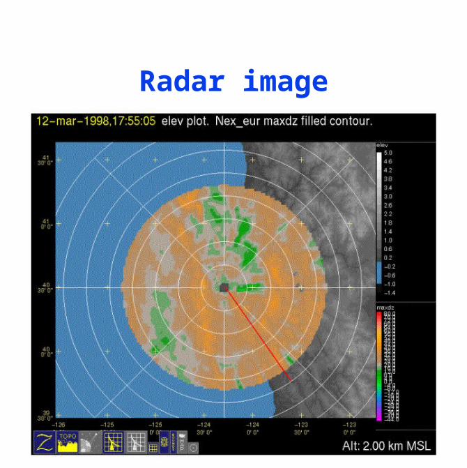
Basic relations, cont.

Radar reflectivity:

Observed radar reflectivity:

€

ZD(t) = cZ D6v(D)N(t)f(D)dD0

∞

∫ ⎛

⎝ ⎜

⎞

⎠ ⎟

€

Z(t) ~ N(ZD (t),σZ2 )

Structure of model

Data: [G|N(D),G] [Z|N(D),Z]

Processes: [N|N,N] [D|t,D]

log GARCH LN

Temporal dynamics: [N(t)|]

AR(1)

Model parameters: [G,Z,N,,D|H]

Hyperparameters: H

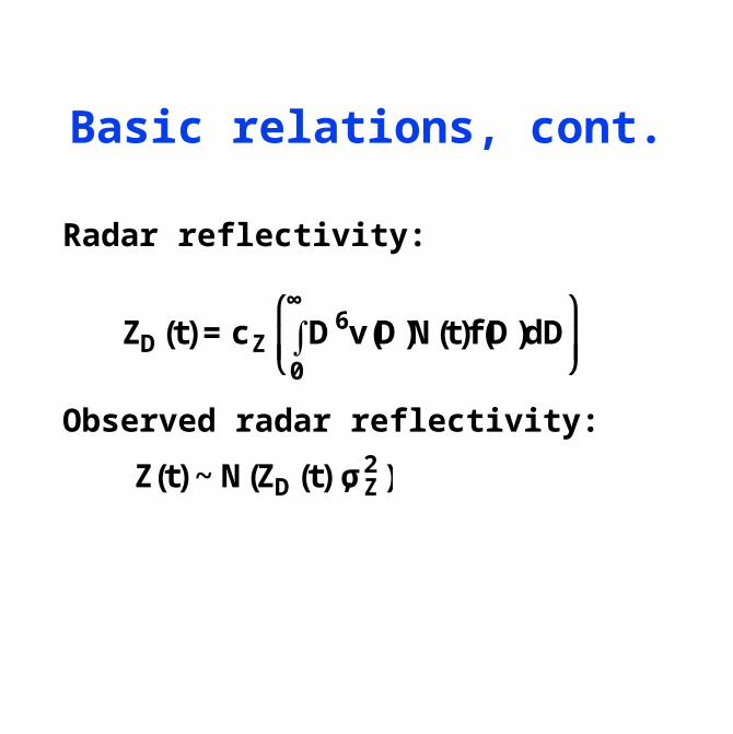
MCMC approach

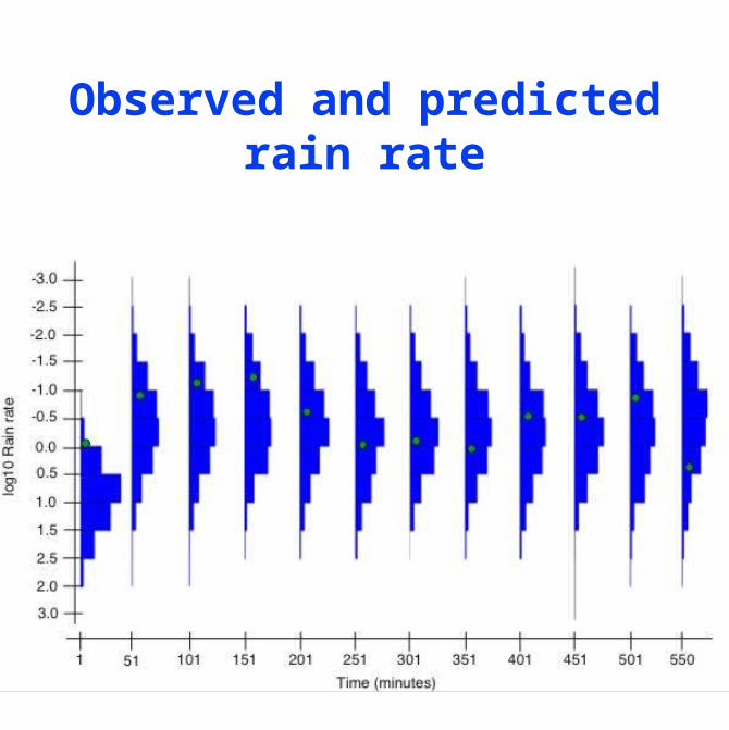
Observed and predicted rain rate

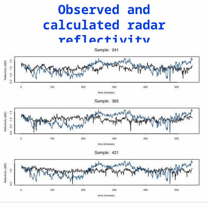
Observed and calculated radar reflectivity

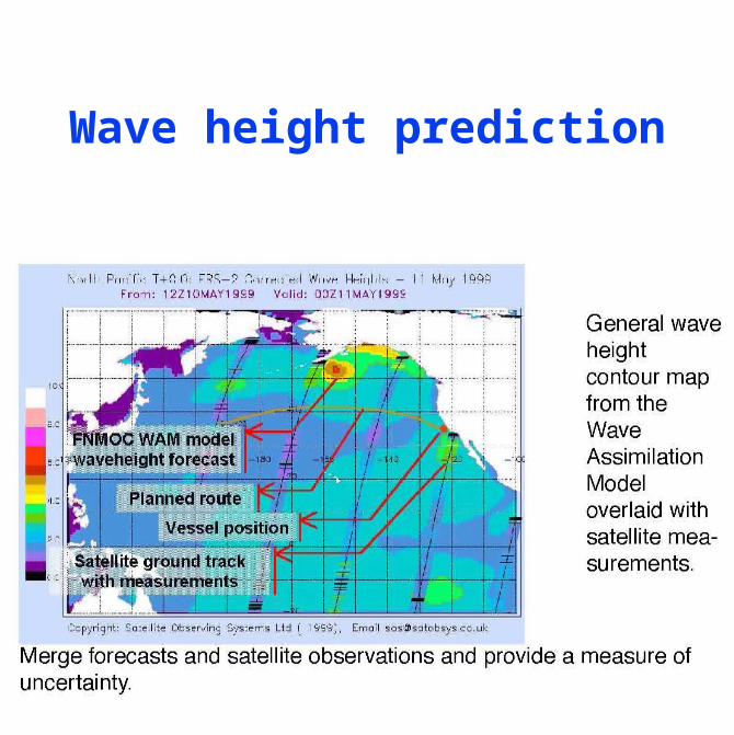
Wave height prediction

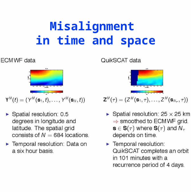
Misalignment in time and space

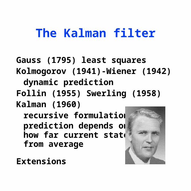
The Kalman filter

Gauss (1795) least squaresKolmogorov (1941)-Wiener (1942)

dynamic predictionFollin (1955) Swerling (1958)Kalman (1960)

recursive formulationprediction depends onhow far current state isfrom average

Extensions

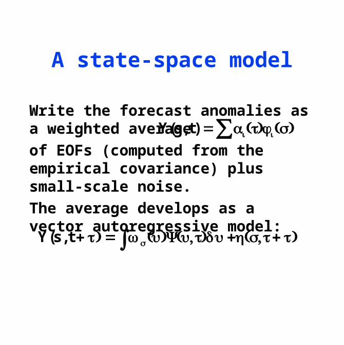
A state-space model

Write the forecast anomalies as a weighted average

of EOFs (computed from the empirical covariance) plus small-scale noise.

The average develops as a vector autoregressive model:

Y(s, t + τ) = ws (u)Y(u, t)du+∫ η(s, t+ τ)

Y(s, t) = ai (t)φi (s)∑

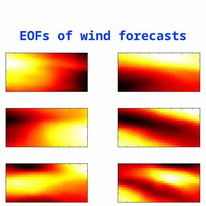
EOFs of wind forecasts

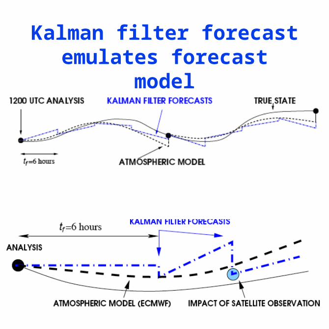
Kalman filter forecast emulates forecast model

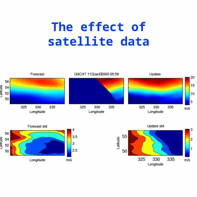
The effect of satellite data

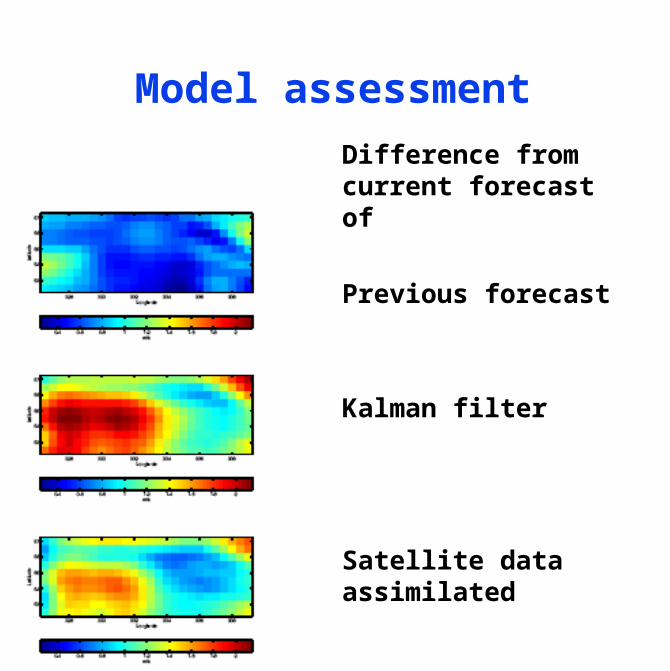
Model assessment

Difference from current forecast of

Previous forecast

Kalman filter

Satellite data assimilated