Embed Size (px)
Citation preview
Smooth-threshold multivariate genetic prediction with unbiased model selection
Masao Ueki* and Gen Tamiya† for Alzheimer’s Disease Neuroimaging Initiative‡
*Biostatistics Center, Kurume University, 67 Asahi-Machi, Ku-rume, Fukuoka 830-0011, Japan
†Tohoku Medical Megabank Organization, Tohoku University, 2-1 Seiryo-Machi, Aoba-Ku, Sendai 980-8573, Japan
Abstract
We develop a new genetic prediction method, smooth-threshold multivariate genetic prediction,
using single nucleotide polymorphisms (SNPs) data in genome-wide association studies (GWASs).
Our method consists of two stages. At the first stage, unlike the usual discontinuous SNP
screening as used in the gene score method, our method continuously screens SNPs based on the
output from standard univariate analysis for marginal association of each SNP. At the second
stage, the predictive model is built by a generalized ridge regression simultaneously using the
screened SNPs with SNP weight determined by the strength of marginal association. Continuous
SNP screening by the smooth-thresholding not only makes prediction stable but also leads to a
closed form expression of generalized degrees of freedom (GDF). The GDF leads to the Stein’s
unbiased risk estimation (SURE) which enables data-dependent choice of optimal SNP screening
cutoff without using cross-validation. Our method is very rapid because computationally expensive
genome-wide scan is required only once in contrast to the penalized regression methods including
lasso and elastic net. Simulation studies which mimic real GWAS data with quantitative and binary
traits demonstrate that the proposed method outperforms the gene score method and genomic best
linear unbiased prediction (GBLUP), and also shows comparable or sometimes improved
performance with the lasso and elastic net being known to have good predictive ability but with
heavy computational cost. Application to whole-genome sequencing (WGS) data from the
Alzheimer’s Disease Neuroimaging Initiative (ADNI) exhibits that the proposed method shows
higher predictive power than the gene score and GBLUP methods.
Keywords
Genetic prediction; marginal association screening; model selection; smooth-thresholding
‡Data used in preparation of this article were obtained from the Alzheimer’s Disease Neuroimaging Initiative (ADNI) database (adni.loni.usc.edu). As such, the investigators within the ADNI contributed to the design and implementation of ADNI and/or provided data but did not participate in analysis or writing of this report. A complete listing of ADNI investigators can be found at: http://adni.loni.usc.edu/wp-content/uploads/howtoapply/ADNIAcknowledgementList.pdf
HHS Public AccessAuthor manuscriptGenet Epidemiol. Author manuscript; available in PMC 2018 March 13.
Published in final edited form as:Genet Epidemiol. 2016 April ; 40(3): 233–243. doi:10.1002/gepi.21958.
Author M
anuscriptA
uthor Manuscript
Author M
anuscriptA
uthor Manuscript
1 Introduction
Genome-wide association study (GWAS) is a popular tool for discovering disease-
susceptibility genes using large number of single nucleotide polymorphisms (SNPs) without
prior knowledge [The Wellcome Trust Case Control Consortium 2007]. Apart from
discovery of susceptibility genes, prediction of individual’s phenotype from high-
dimensional genetic information, termed as a genetic prediction, is an important task for
personalized medicine. Currently, researchers are exploring the most effective way of
building genetic prediction models [Purcell et al. 2009, Evans et al. 2009]. In this paper, we
develop a new statistical approach, smooth-threshold multivariate genetic prediction, for
building genetic predictive models with input of large-scale genome-wide SNPs data.
We consider standard multiple regression model but with high-dimensional predictor
variables. To be specific, y = (y1, . . . , yn)T represent response variables of individual’s
phenotype data modeled by a conditional distribution given predictor variables X = (X1, . . . ,
Xp) observed for n individuals, in which Xj = (x1,j, . . . , xn,j)T for j ∈ M = {1, . . . , p}. The
conditional expectation of yi given xi = (xi,1, . . . , xi,n) is assumed to be a linear combination
η{E(yi|xi)} = xiβ, where η is some known monotone function and β is a vector of regression
coefficients. In this paper, we consider linear regression with identity map η for quantitative
trait such as clinical characteristics, and logistic regression with logit function η for binary
trait such as affected/unaffected status. Each Xj is either genotype at a SNP site or other
covariate such as sex, age, body mass index (BMI), smoking status, alcohol consumption
and principal components for population stratification [Price et al. 2006]. Each SNP can take
one of three possible genotypes, gg, gG and GG, where g and G denote minor and major
alleles at the SNP site, respectively. If Xj represents the observed count of minor allele g at a
SNP site, Xj takes a value from {0, 1, 2}. Under the Hardy–Weinberg equilibrium (HWE),
the observed count of minor allele g at each SNP follows a binomial distribution with
parameter f ∈ [0, 0.5] called a minor allele frequency (MAF), i.e. frequency of the minor
allele g in general population. Quality controls (QCs) are often conducted to remove low-
quality SNPs by checking HWE and missing rates as well as low MAF SNPs. Even after
those QCs, large number of SNPs still remain. Since sample sizes are usually far less than
the number of SNPs, the predictive modeling in GWAS faces the p ≫ n problem (e.g. Fan
and Lv [2008]). The p ≫ n condition hampers multiple regression that fits simultaneously
using p predictors X.
Standard GWAS analysis conducts marginal association scan between y and each Xj
independently, i.e. a univariate analysis which tests the slope parameter in univariate
regression model [The Wellcome Trust Case Control Consortium 2007, Yamagata University
Genomic Cohort Consortium 2014], followed by multiple test using a Bonferroni correction
with a stringent significance level (e.g. p-value less than 5 × 10⁻⁸) in order to control the rate
of false positive findings. Meanwhile, suppose that X does not include covariates and
consists of SNPs only. Let Tj(y, X) represent a non-negative test statistic for testing
association between jth SNP Xj and y as a function of y and X, and the corresponding
inclusion threshold be t > 0. For example, t is a chi-squared quantile at a given p-value cutoff
for chi-squared test statistics Tj(y, X). The resulting SNP set from a marginal association
screening at a threshold t is defined by A = {j ∈ M : Tj(y, X) > t}. Purcell et al. [2009]
Ueki and Tamiya Page 2
Genet Epidemiol. Author manuscript; available in PMC 2018 March 13.
Author M
anuscriptA
uthor Manuscript
Author M
anuscriptA
uthor Manuscript
proposed a gene score method which simply averages each genotype data weighted by
estimated effect size for each SNP in A. Warren et al. [2013] consider multiple regression
for SNPs in A, called a multivariate gene score method.
In the purpose of prediction, the cutoff t can be chosen in terms of prediction ability.
However, evaluating prediction ability is not straightforward unlike in traditional setting
without screening. It is known that, the screening invalidates traditional statistical
procedures, called an winner’s curse effect [Zollner and Pritchard 2007, Zhong and Prentice
2008, Ghosh et al. 2008]. Analogous problem arises in the context of prediction modeling.
Actually, simulation studies as well as examination on real GWAS datasets reported that
screening leads to overfitting [Kooperberg et al. 2010]. In Supplementary Material, we show
that the screening can deflate the residual sum of squares (RSS) compared with the RSS
without screening, so that the RSS becomes too optimistic. Since screening complicates the
behavior of RSS, naive use of RSS is unwarranted in measuring prediction ability. Instead,
we can use cross-validation (or sample splitting) which divides the training data into two
parts, one of which is used for ranking SNPs and remaining is used to construct a predictive
model [Purcell et al. 2009, Kooperberg et al. 2010, Wray et al. 2013, Wei et al. 2013].
Purcell et al. [2009] choose an optimal inclusion cutoff by cross-validation.
Although cross-validation takes into account of the screening, reduced sample sizes in
training stage may lose predictive power [Dudbridge 2013], which is a severe concern when
sample sizes are small. Five or ten-folds cross-validation is commonly used in model
selection. For example, the SparSNP program [Abraham et al. 2012] implementing
penalized regression methods, the lasso and elastic net, searches for entire genome-wide
SNPs data without SNP screening. SparSNP selects the tuning parameter by k-fold cross-
validation with default setting of k = 10. Repeated genome-wide scans needed at each
candidate tuning parameter and multiple runs of model fit-ting in each fold increase
computational cost. For large-scale data such as the whole-genome sequencing (WGS) data,
heavy computational cost critically limits the applicability although penalized methods are
known to give better predictive power than the simpler gene score method [Purcell et al.
2009].
In this paper, we develop a new predictive modeling approach, a smooth-threshold
multivariate genetic prediction, which is really applicable to large-scale genome-wide data
such as WGS data while preserving high prediction ability. Our method consists of two
stages. At the first stage, our method continuously screens SNPs based on the output from
standard univariate analysis for marginal association of each SNP. At the second stage, the
predictive model is built by a generalized ridge regression simultaneously using the screened
SNPs with SNP weight determined by the strength of marginal association reflecting the
uncertainty of inclusion. Since the final predictive model is essentially built in multiple
regression model as in the sure independence screening [Fan and Lv 2008], the correlations
between predictor variables are accounted for (See also Warren et al. [2013]). Marginal
association signal is used only for penalizing each regression coefficient. Our method is very
rapid because computationally expensive genome-wide scan is required only once in
contrast to the penalized methods which need genome-wide scan several times. Our proposal
can be seen as a smoothed version of multiple regression after single SNP-GWAS screening
Ueki and Tamiya Page 3
Genet Epidemiol. Author manuscript; available in PMC 2018 March 13.
Author M
anuscriptA
uthor Manuscript
Author M
anuscriptA
uthor Manuscript
of predictor variables at some p-value cutoff, in which the discontinuous process in
screening is replaced by a continuous function. The resulting continuity makes the
prediction stable in the sense of Breiman [1996]. The continuity in SNP screening also leads
to a closed form expression of generalized degrees of freedom (GDF) [Ye 1998, Efron
2004], and allows an application of Stein’s unbiased risk estimation (SURE) [Stein 1981].
While the Mallows’ Cp [Mallows 1973] with the usual degrees of freedom is no longer
unbiased model selection criterion due to the effect of screening, we can readily construct an
unbiased Cp-type model selection criterion using the GDF [Ye 1998, Efron 2004]. It allows
data-dependent choice of optimal SNP inclusion cutoff without relying on cross-validation.
The effect of screening is properly accounted for by the SURE’s unbiasedness. Since no
cross-validation is needed, computationally expensive genome-wide scan is required only
once in ranking SNPs. We also extend to generalized linear models and propose a
loglikelihood-based Cp-type model selection criterion. Simulation studies which mimic real
SNP-GWAS data for both quantitative and binary traits show that the proposed method gives
better performance than gene score and genomic best linear unbiased prediction (GBLUP)
[Goddard et al. 2009, Yang et al. 2011, Lee et al. 2011, Makowsky et al. 2013, de Los
Campos et al. 2013, Speed and Balding 2014] and attains a comparable or sometime
improved prediction performance with the lasso and elastic net in SparSNP program.
Application to large-scale WGS data from Alzheimer’s Disease Neuroimaging Initiative
(ADNI) exhibits that the proposed method gives higher predictive performance than both the
gene score and GBLUP methods.
2 Materials and Methods
Here we consider linear multiple regression model, y = μ + ε, where μ = E(y|X) = Xβ, ε ~ N(0, σ2In), X is a p-dimensional design matrix and β is the corresponding p regression
coefficients. Since p is much larger than n in typical GWAS data, some dimensionality
reduction is required. Sparsity assuming that many components of β are zero would be a
realistic assumption. If susceptible SNPs show relatively large marginal signal, marginal
association screening effectively reduces the dimensionality. The gene score method [Purcell
et al. 2009] and its multivariate generalization [Warren et al. 2013] use upper-ranked SNPs
in marginal association, A = {j ∈ M : Tj(y, X) > t}, for a given cutoff value t > 0. Although
dimensionality is effectively reduced, discontinuity in y present in the screening process in
A may incur instability of prediction, i.e. small change in data can make large changes in the
prediction [Breiman 1996]. See also Fan and Li [2001]. To address the discontinuity issue,
we use a smooth-thresholding proposed by Ueki [2009]. To be specific, we propose to
estimate the regression coefficients by
(1)
where Ac indicates the complement set of A, ǦA = {(I|A|−ĎA)(ΣAA+λI|A|)+τĎA}−1, Σ =
XTX, ΣAA = (Σjk)j∈A,k∈A, γ and τ are non-negative tuning parameters and λ > 0 is a small
Ueki and Tamiya Page 4
Genet Epidemiol. Author manuscript; available in PMC 2018 March 13.
Author M
anuscriptA
uthor Manuscript
Author M
anuscriptA
uthor Manuscript
constant to avoid singularity of ǦA. The corresponding prediction of yi is then .
Here Ďj is an adaptive lasso smooth-thresholding function defined by
(2)
Since Ďj = 1 if and only if Tj(y, X) ≤ t, the screened set A with Ďj is the same as that with D̂j
= 1{Tj(y,X)≤t}, where 1{·} denotes the indicator function. It can be seen that Ďj replaces the
discontinuous screening process D̂j by a continuous function. As a result, μ̌i(y) turns out to
be continuous in y.
The regression coefficient for the screened set in (1), β̌A, can be seen as a solution to
(3)
with WA = diag(Wj : j ∈ A) where Wj = λ + τ Ďj/(1 − Ďj), which is the minimizer of a
generalized ridge regression loss, , with respect to βA. Ridge
weight for each predictor variable, Wj, represents uncertainty of marginal association
screening. If the marginal association is very weak, we have Ďj ≈ 1 and large Wj, then the
corresponding regression coefficient is strongly shrunken towards zero. If the marginal
association is strong, we have Ďj ≈ 0 and Wj ≈ λ, then the corresponding regression
coefficient is less penalized. From the fact that the winner’s curse effect produces larger
selection bias for small regression coefficient [Zhong and Prentice 2008], it is expected that
the above penalization decreases the selection bias.
Predictive power largely depends on the choice of t. It may be done using cross-validation
by dividing a dataset into test and training samples [Warren et al. 2013]. Cross-validation
takes into account sampling variability due to the screening [Wray et al. 2013, Wei et al.
2013]. However, repeated genome-wide scans to obtain the screened set A needed in cross-
validation incurs computational burden. It is also concerned that the reduction in training
sample sizes decreases the predictive power of the model [Dudbridge 2013]. Instead of
cross-validation, we propose a Cp-type criterion based on SURE using GDF. The continuity
of μ̌i(y) in y leads to a closed-form expression of GDF. In what follows, we consider p-value
cutoff α instead of t by a one-toone transformation t = F−1(1 − α), where F−1 is a quantile
function of the distribution of Tj(y, X) under the null hypothesis of no marginal association
such as F or χ2 distribution. An optimal α is determined by minimizing the Cp-type criterion
within a range of α for search, [αmin, αmax]. The proposed procedure is outlined at the end
of this section. It is noteworthy that the computational intensive genome-wide scan is
required only once in the single-SNP association screening at Step 1. Subsequent Steps 2–4
are performed on the reduced set of SNPs whose single-SNP association p-value is less than
αmax.
Ueki and Tamiya Page 5
Genet Epidemiol. Author manuscript; available in PMC 2018 March 13.
Author M
anuscriptA
uthor Manuscript
Author M
anuscriptA
uthor Manuscript
It is shown that in Supplementary Material that expectation of the Cp-type criterion equals to
. The selection bias in RSS due to screening mentioned above is
accounted for by this unbiasedness property. Consequently, model selection with the Cp-type
criterion is expected to work properly. In principle, the two tuning parameters (γ and τ)
other than α may be selected by the Cp-type criterion. However, simulation studies and our
experiences in real data applications suggested that better predictive power is attained with
some fixed values of γ and τ, possibly, because the reduction of tuning parameters decreases
sampling variability due to search of optimal prediction model. Specifically, we use fixed
values of γ = 1 and throughout. Consequently, we consider single tuning
parameter α to be optimized. The Cp-type criterion contains σ2 which is often unknown. A
surrogate estimate of σ2 is given in Supplementary Material. More details of this section
including formulas, derivations, extension to generalized linear models and additional
descriptions are given in Supplementary Material.
Outline of algorithm
Step 1. Perform single-SNP association analysis for p SNPs.
Step 2. Screen SNPs whose single-SNP association p-value is less than αmax.
Step 3. Fix γ and τ as suggested in main text, and select an optimal α from candidate
values in [αmin, αmax] by minimizing the Cp-type criterion:
Explicit formulas are given in Supplementary Material.
Step 4. Compute β̌ by (1) using the selected α.
3 Results
3.1 Simulation results
To examine the performance of the proposed method, we conducted simulation studies with
artificial data which mimic real SNP-GWAS data. Simulations were based on sampling
individuals from general population where HAPGEN v2.2.0 [Su et al. 2011] was used with
input of haplotype data consisting of 73,832 SNPs on chromosome 10 from HapMap3 east
Asian population (JPT+CHB). In our experiments, we compared the proposed method,
lasso, elastic net, GBLUP and gene score (GS) methods. For lasso and elastic net, we used
SparSNP program, in which default parameters of 10 × 10 cross-validation were used for
tuning. For elastic net, a fixed L2 penalty of λ2 = 1 was used throughout as in Abraham et al.
[2013]. For GBLUP, we used GCTA v1.24.4 [Yang et al. 2011]. For GS, we used PRSice
v1.23 [Euesden et al. 2015] with default setting with clumping, in which samples are
randomly divided into two datasets with 1:9 proportion (1/10 for target data and 9/10 for
training data) for selecting optimal p-value cutoff from {0.01, 0.02, , . . . , 0.5}.
Ueki and Tamiya Page 6
Genet Epidemiol. Author manuscript; available in PMC 2018 March 13.
Author M
anuscriptA
uthor Manuscript
Author M
anuscriptA
uthor Manuscript
Quantitative traits—Using HAPGEN v2.2.0, n individuals from general population were
sampled. Then, a quantitative phenotype yi for each individual i = 1, . . . , n was generated
according to the linear regression model, yi = μi + εi, where X0,iβ0, εi ~ N (0, σ2) is an
independent Gaussian noise, X0,i is a vector of p0 causal SNPs, a subset from 73,832 SNPs
coded 0, 1, 2 for minor allele counts in the generated genotype data and β0 is the p0 true
regression coefficients for causal SNPs. In our simulations, p0 was set in advance, then p0
causal SNPs were randomly assigned from 73,832 SNPs.
We consider both oligogenic and polygenic architectures as follows. For oligogenic scenario,
we set n = 1000, and each of p0 elements of β0, β0,j, was randomly chosen from three values
{0.2, 0.1, 0.05}. We repeated simulations 50 times and examined the following four models:
Model O1, p0 = 10, σ2 = 1 (h2 = 0.13); Model O2, p0 = 10, σ2 = 2 (h2 = 0.07); Model O3, p0
= 50, σ2 = 1 (h2 = 0.47); Model O4, p0 = 50, σ2 = 2 (h2 = 0.31). Here h2 denotes the narrow
sense heritability averaged over 50 replicates. For each replicate, the narrow sense
heritability is computated by where and qj is the
MAF for each of p0 causal SNPs. For polygenic scenario, we set n = 5000, and each of p0
elements of β0 was set as and ξj was independently and identically
generated from a double exponential (or Laplace) distribution with zero median and
scale parameter. We then set σ2 = 1 − h2 so that . We repeated
simulations 20 times and examined the following six models: Model P1, p0 = 100, h2 = 0.3;
Model P2, p0 = 100, h2 = 0.1; Model P3, p0 = 100, h2 = 0.05; Model P4, p0 = 200, h2 = 0.3;
Model P5, p0 = 200, h2 = 0.1; Model P6, p0 = 200, h2 = 0.05.
In all simulations, we randomly chose 100 subjects for test samples, say Nte, and set the
remaining Ntr = {1, . . . , n} \ Nte as training samples. Predictive power was evaluated by
whether the proposed method trained on the training samples predicts the phenotype of test
samples. Using the proposed unbiased model selection criterion, an optimal p-value cutoff
was chosen from 50 equally-spaced candidate values between αmax = 9n/(p log n) and αmin
= 5 × 10⁻⁸ in −log10 scale, i.e. αmax = α(1) > α(2) > ··· > α(50) = αmin We used PLINK --
assoc option to compute marginal association p-values, and then screened SNPs whose p-
value is less than αmax. Since the PLINK’s association p-value is based on Wald test, we
recomputed F-test statistics (Tj(y, X) described in Supplementary Material) for the above
screened SNPs. In practice, each p-value cutoff, αk, was converted to a threshold for Tj(y,
X)s to be optimized, t(k) = F−1(1 − α(k)), where F−1 denotes the quantile function of F (1, n − 1)-distribution. The optimal cutoff was determined from t(1) < t(2) <···< t(50) which
minimizes the Cp-type criterion.
Resulting prediction errors, PSEtr = |Ntr|−1 Σi∈Ntr E{(y0,i − μ̌tr,i)2} = |Ntr|−1Σi∈NtrE{(μi −
μ̌tr,i)2} + σ2, and PSEte =|Nte|−1 Σi∈NteE{(yi − μ̌tr,i)2}, are plotted as a function of α in
Figures 1 (oligogenic scenario) and 2 (polygenic scenario) averaged over replicates. Here,
μ̌tr,i = Xiβ̌tr denotes the predicted value for ith sample using the regression coefficients β̌tr by
the proposed smooth-threshold multivariate genetic prediction based on training samples,
while y0,i is an independent future observation from the same distribution of yi given Xi, i.e.,
μi + ε0,i, with Gaussian noise ε0,i ~ N (0, σ2) independent of εi and μi = X0,iβ0. It can be
Ueki and Tamiya Page 7
Genet Epidemiol. Author manuscript; available in PMC 2018 March 13.
Author M
anuscriptA
uthor Manuscript
Author M
anuscriptA
uthor Manuscript
seen that the proposed Cp-type criterion indeed possesses the unbiasedness to the true mean
squared prediction error for training samples, PSEtr, across various p-value cutoff values.
Each curve had a minimum at some optimal cutoff value and formed a convex function.
The regression coefficients β̌tr estimated on training samples were used for predicting
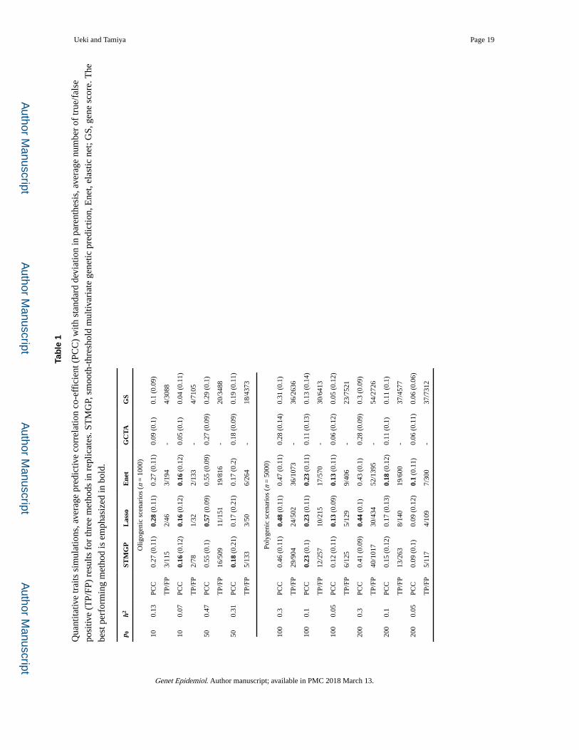
phenotype value of test samples. In Table 1, the predictive power was evaluated by the
predictive correlation coefficient (PCC) which is the Pearson’s correlation between the
predicted value and the actual phenotype of test samples. For the proposed method, the
predicted values for test samples were computed at an optimal p-value cutoff value selected
by minimizing the proposed Cp-type criterion. From the PCCs given in Table 1, the
prediction performance of lasso and elastic net was comparable with the proposed method.
On the other hand, the GBLUP and GS showed much lower performance than the proposed
method, lasso and elastic net in some oligogenic scenarios. In polygenic scenarios, the
proposed method gave slightly lower performance than the lasso and elastic net. We also
conducted additional polygenic simulations assuming low heritabilities. The results given in
Supplementary Material show that all methods gave very low predictive performance,
agreeing with the observation in Warren et al. [2013].
For the proposed method, lasso, elastic net and gene score, Table 1 gives the average number
of true and false positives, respectively, defined by that non-zero coefficients from each
method are truly and falsely causal SNPs. Overall, all methods yielded large number of false
positives, which would result from that the assumed effect sizes were small relative to the
noise.
Binary traits—For simulations of binary traits, case-control data were used for training
samples to build a predictive model, and then the predictive model was tested through
independent test samples from general population. We consider both oligogenic and
polygenic architectures as follows. For oligogenic scenario, 1000 balanced case-control
samples (500 cases and 500 controls) for training and 1000 samples for test were considered.
Case-control samples were collected based on repeated sampling from general population as
described below in detail. A binary phenotype yi ∈ {0, 1} of each individual from general
population was generated according to the logistic regression model μi = P (yi = 1|Xi) = 1/{1
+ exp(−θi)}, where Xi denotes a realization of the individual i’s SNPs vector with additive
coding as in the quantitative trait simulation, θi = Xiβ0 + b0, b0 is the baseline regression
coefficient and β0 denotes p0 true regression coefficients. p0 causal SNPs were randomly
chosen from all 73,832 SNPs, and then, 0,1,2 coding was carried out according to the minor
allele count in reference haplotype data. Then, p0 regression coefficients β0 were randomly
assigned from three values {(m/2) log 1.1, (m/2) log 1.2, (m/2) log 1.5}, with a constant
parameter m. The following four models were considered: Model O5, p0 = 10, m = 2, b0 =
−4 (h2 = 0.05); Model O6, p0 = 10, m = 3, b0 = −5 (h2 = 0.11); Model O7, p0 = 50, m = 0.8,
b0 = −4 (h2 = 0.04); Model O8, p0 = 50, m = 1.2, b0 = −5 (h2 = 0.09). Here h2 denotes the
narrow sense heritability averaged over 50 replicates just like the quantitative traits
simulations using except that σ2 = p2/3 which is the variance of logistic
distribution with unit scale (i.e. liability follows logistic distribution rather than Gaussian).
For polygenic scenario, 5000 balanced case-control samples (2500 cases and 2500 controls)
Ueki and Tamiya Page 8
Genet Epidemiol. Author manuscript; available in PMC 2018 March 13.
Author M
anuscriptA
uthor Manuscript
Author M
anuscriptA
uthor Manuscript
for training and 1000 samples for test were considered. First we generated liability from
Gaussian distribution as done in the polygenic quantitative traits simulations, in which mean
of liability is adjusted to be zero. Then, we assigned yi = 1 if the liability exceeds Φ−1(1 −
K0) and 0 otherwise, where K0 = 0.1 and Φ−1 is the standard normal quantile function. We
repeated simulations 20 times and examined the following six models: Model P7, p0 = 100,
h2 = 0.3; Model P8, p0 = 100, h2 = 0.1; Model P9, p0 = 100, h2 = 0.05; Model P10, p0 = 200,
h2 = 0.3; Model P11, p0 = 200, h2 = 0.1; Model P12, p0 = 200, h2 = 0.05, which correspond
to the models with liability generated from Models P1,. . . ,P6.
n0 cases and n1 controls data were generated as follows. First, 1000 individuals were
sampled from general population using HAPGEN as described in earlier of this subsection.
In each sampling, case/control status was assigned for each individual according to the
specified model. Since the number of cases was in general smaller than that of controls, a
subset of controls with the same number of cases occurred was randomly chosen. As a
result, cases and controls with equal numbers were stored. The above process was continued
until total sample size reaches to the desired number. In addition, 1000 individuals were
generated from general population using HAPGEN, and a case/control status was assigned
from the specified regression model. The 1000 individuals were used for test samples.
Using the proposed (approximate) unbiased model selection criterion, an optimal p-value
cutoff was chosen from 50 equally-spaced candidate values between αmax = 3n/(p log n) and
αmin = 5 × 10⁻⁸ in −log10 scale. Marginal association screening was conducted as in the
quantitative trait simulations except that the score test statistic was used for Tj(y, X) instead
of the F-test statistic and that F −1 is the quantile function of χ2 distribution with one degree
of freedom. As in Figures 1 and 2, Figures 3 and 4 give prediction errors measured by −2× loglikelihood, PLtr = |Ntr|−1Σi∈Ntrq{(μi, θ̌tr,i) and PLte = |Nte|−1Σi∈Nteq{(yi, θ̌tr,i), as a
function of α. Here θ̌tr,i = Xiβ̌tr denotes the predicted value for ith sample using the
regression coefficients β̌tr by the proposed smooth-threshold multivariate genetic prediction
learned on the training samples. From Figures 3 and 4, the proposed Cp-type criterion
appeared to be close to the true mean prediction −2× loglikelihood. Each curve had a
minimum at some optimal cutoff value and formed a convex function.
The regression coefficients β̌tr estimated on training samples were used to predict the
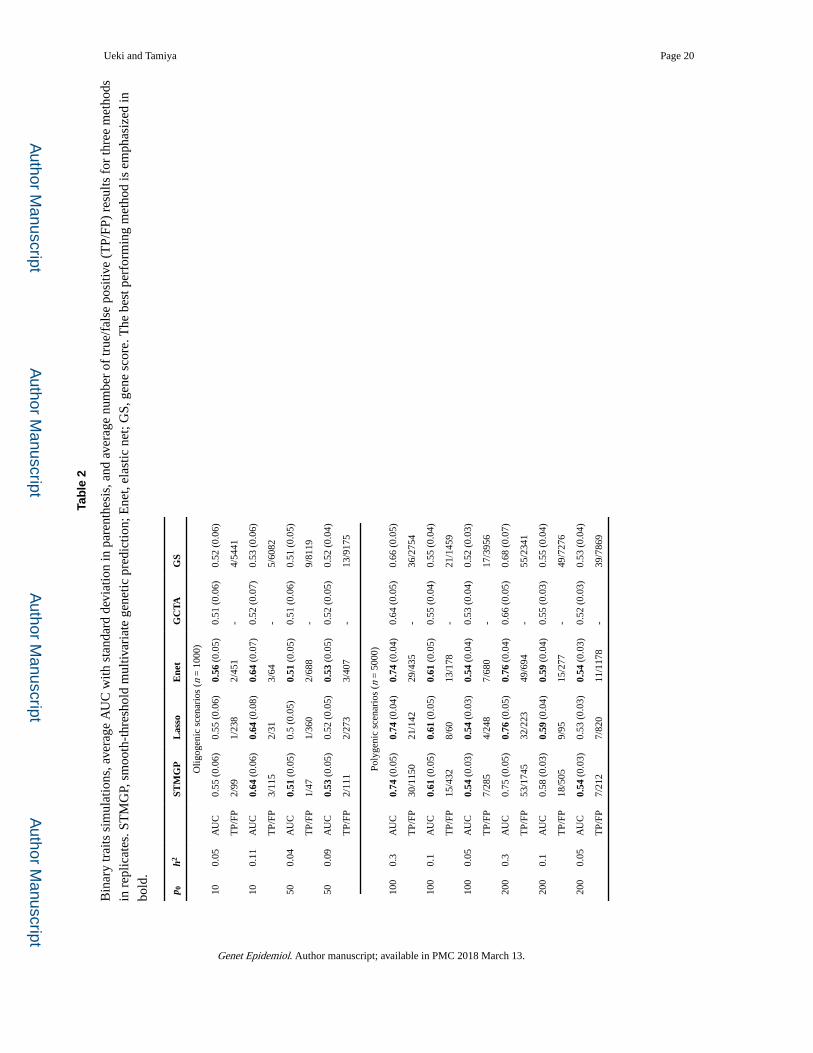
phenotype of test samples. In Table 2, the predictive power was evaluated by the area under
a receiver operating characteristic curve (AUC). For the proposed method, the mean
prediction errors for test samples were computed using an optimal p-value cutoff value
selected by minimizing the proposed Cp-type criterion. Resulting prediction performances
were given in Table 2. The proposed method, lasso and elastic net, showed comparable
predictive power. On the other hand, the GBLUP and GS showed much lower performance
than the proposed method, lasso and elastic net in some oligogenic scenarios. In
Supplementary Material, we also conducted additional polygenic simulations assuming low
heritabilities. The results are similar to that in quantitative traits simulations. For the
proposed method, lasso, elastic net and gene score, average number of true and false
positives were compared in Table 2. As in quantitative traits simulations, large number of
false positives resulted in all methods.
Ueki and Tamiya Page 9
Genet Epidemiol. Author manuscript; available in PMC 2018 March 13.
Author M
anuscriptA
uthor Manuscript
Author M
anuscriptA
uthor Manuscript
3.2 Application to ADNI-WGS data
We applied our proposed method to ADNI-WGS dataset obtained from the publicly
available data of the Alzheimer’s Disease Neuroimage Initiative (ADNI) database
(adni.loni.usc.edu). The ADNI was launched in 2003 as a public-private partnership, led by
Principal Investigator Michael W. Weiner, MD. The primary goal of ADNI has been to test
whether serial magnetic resonance imaging (MRI), positron emission tomography (PET),
other biological markers, and clinical and neuropsychological assessment can be combined
to measure the progression of mild cognitive impairment (MCI) and early Alzheimer’s
disease (AD). For up-to-date information, see www.adni-info.org. ADNI is an ongoing
longitudinal study with the primary purpose of exploring the genetic and neuroimaing
information associated with late-onset Alzheimer’s disease (LOAD). The study recruited
elderly subjects older than 65 years of age consisting about 400 subjects with mild cognitive
impairment (MCI), about 200 subjects with Alzheimer’s disease (AD), and around 200
healthy controls (normal). Each subject was followed for at least 3 years. During the study
period, the subjects were assessed with magnetic resonance imaging (MRI) measures and
psychiatric evaluation to determine the diagnosis status at each time point.
We used high coverage WGS data called using Broad best practices (BWA & GATK
HaplotypeCaller). From the ADNI-WGS data, we extracted 8,657,877 single nucleotide
variant (SNV) sites. In our analysis, we used 713 non-Hispanic Caucasian samples
excluding one of pairs showing cryptic relatedness implied by the PLINK’s pairwise π̂
statistic [Purcell et al. 2007] greater than 0.125. Consequently, the total numbers of subjects
with the current status of normal, MCI and AD were 245, 426 and 42, respectively. We
separately considered three different definitions of phenotypes: (i) normal (= 1), MCI (= 2)
and AD (= 3) as quantitative traits, (ii) normal (= 1), MCI (= 2) and AD (= 2) as binary
traits, (iii) normal (= 1), MCI (= 1) and AD (= 2) as binary traits. We also considered two
kinds of adjustments for covariates: (a) sex and age, (b) sex, age, year of education (EDU)
and family history (FH). For family history, we coded 1 if any of subject’s mother, father
and siblings had affected AD, and 0 otherwise. We chose the above covariates because of the
known influence on AD.
We used the proposed smooth-threshold multivariate genetic prediction, GBLUP and GP
methods for building prediction model. In all three methods, covariates were adjusted. Since
the ADNI-WGS data include large number of SNVs, we did not apply the lasso and elastic
net in SparSNP due to prohibitive computational cost.
First, we randomly divided 718 samples into ten groups with roughly equal size. Then, one
of ten groups was set as test samples and remaining was set as training samples.
Consequently, we had ten combinations of test/training samples (i.e. 10-fold cross-
validation). For each of ten combinations, we built a prediction model based on training
samples, and predict phenotype data of test samples by the prediction model. For each
training data, we used SNVs with MAF > 1% and with missing genotype rates < 10% in
building prediction model. For the proposed smooth-threshold multivariate genetic
prediction, we searched for an optimal p-value cutoff from 50 equally-spaced points between
Ueki and Tamiya Page 10
Genet Epidemiol. Author manuscript; available in PMC 2018 March 13.
Author M
anuscriptA
uthor Manuscript
Author M
anuscriptA
uthor Manuscript
αmax = 3000/8657877 and αmin = 5 × 10⁻⁸ in −log10 scale while we fixed γ = 1 and
.
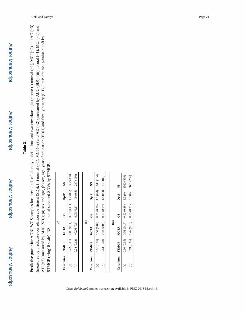
In Table 3, predictive power for each three methods averaged over ten test/training datasets
was given where standard deviation was given in parenthesis. In (i), phenotype data were
treated as a quantitative trait, and the predictive power was evaluated by PCC. In (ii) and
(iii), phenotype data were treated as binary traits, and the predictive power was evaluated by
AUC. The proposed method showed the best predictive power among three competing
methods as observed in simulation studies.
In Table 3, we also provided selected optimal p-value cutoff values in −log10 scale and
number of screened SNVs by the proposed method averaged over 10 test/training datasets.
We note that, in (iii), the proposed Cp-type criterion failed to identify the optimal p-value
cutoff in the sense that the minimum value of the criterion was always at the boundary for
search, 3000/8657877 (or 3.5 in −log10 scale), as seen in the zero standard deviation in Table
3. It implies that the results for the proposal in Table 3 were suboptimal despite the higher
predictive power than the competing methods. One reason of failing to select an optimal p-
value cutoff in (iii) would be the small sample size in cases, which made the estimation of
Cp-type criterion highly unstable. On the other hand, for (i) and (ii), the proposed Cp-type
criterion could take an optimal p-value cutoff which was not at the boundary, i.e. the
selection of optimal p-value cutoff was successful.
Our proposed method gave higher predictive power than the GBLUP and gene score as
observed in our oligogenic simulations. In our analyses, we included SNVs on APOE
(Apolipoprotein E) gene known to have large contribution to developing AD. For such
disease, the genetic architecture may be approximated by sparse models considered in the
oligogenic scenarios. We note that the predictive power is still insufficient for practical
genetic prediction. Recent studies [Chatterjee et al. 2013, Dudbridge 2013] under
infinitesimal models [Fisher 1918] state that more sample sizes are needed to construct
accurate predictive models. It is expected that increasing sample sizes improve the predictive
power. Our proposed approach is general and has a potential to apply to various high-
dimensional problems based on multiple linear regression.
4 Conclusion
In this paper, we presented a new efficient predictive modeling using smooth-threshold
multivariate genetic prediction. The method can be seen as a smoothed version of multiple
regression after marginal association screening or multivariate gene score [Warren et al.
2013]. Advantages of continuity include (i) stabilizing prediction and (ii) applicability of Cp-
type unbiased model selection criterion. For (i), through extensive simulation studies, the
predictive power of the proposed method had a comparable performance with the
contemporary shrinkage methods, lasso and elastic net, which has large computational cost.
For (ii), the unbiasedness property of Cp-type criterion was confirmed by simulation studies.
The use of Cp-type criterion allows to tune an optimal p-value cutoff without using cross-
validation. We are unnecessarily to be concerned on training sample sizes.
Ueki and Tamiya Page 11
Genet Epidemiol. Author manuscript; available in PMC 2018 March 13.
Author M
anuscriptA
uthor Manuscript
Author M
anuscriptA
uthor Manuscript
The fact that the proposed method requires computationally intensive genome-wide scan
only once makes computation more rapid. It is advantageous for WGS data which include
large number of variants. An R code which implements the proposed method with input of
PLINK-binary format data and summary statistics such as single-SNP association p-values
is available from the authors upon request.
Supplementary Material
Refer to Web version on PubMed Central for supplementary material.
Acknowledgments
The authors would like to thank a referee, Dr. Doug Speed and Prof. Sadanori Konishi for helpful comments that led to significant improvement of the paper. Data collection and sharing for this project was funded by the Alzheimer’s Disease Neuroimaging Initiative (ADNI) (National Institutes of Health Grant U01 AG024904) and DOD ADNI (Department of Defense award number W81XWH-12-2-0012). ADNI is funded by the National Institute on Aging, the National Institute of Biomedical Imaging and Bioengi-neering, and through generous contributions from the following: AbbVie, Alzheimer’s Association; Alzheimer’s Drug Discovery Foundation; Araclon Biotech; BioClinica, Inc.; Biogen; Bristol-Myers Squibb Company; CereSpir, Inc.; Eisai Inc.; Elan Pharmaceuticals, Inc.; EliLilly and Company; EuroIm-mun; F. Hoffmann-La Roche Ltd and its affiliated company Genentech, Inc.; Fujirebio; GE Healthcare; IXICO Ltd.; Janssen Alzheimer Immunotherapy Research & Development, LLC.; Johnson & Johnson Pharmaceutical Research & Development LLC.; Lumosity; Lundbeck; Merck & Co., Inc.; Meso Scale Diagnostics, LLC.; NeuroRx Research; Neurotrack Technologies; No-vartis Pharmaceuticals Corporation; Pfizer Inc.; Piramal Imaging; Servier; Takeda Pharmaceutical Company; and Transition Therapeutics. The Cana-dian Institutes of Health Research is providing funds to support ADNI clinical sites in Canada. Private sector contributions are facilitated by the Foundation for the National Institutes of Health (www.fnih.org). The grantee organization is the Northern California Institute for Research and Education, and the study is coordinated by the Alzheimer’s Disease Cooperative Study at the University of California, San Diego. ADNI data are disseminated by the Laboratory for Neuro Imaging at the University of Southern California. This work was carried out under the ISM General Cooperative Research 1 (2015-ISM-CRP-1013) and was partially supported by a Grant-in-Aid for Young Scientist (B) (25870074) and Grants-in-Aid for Scientific Research (C) (25330049 and 25460403).
References
Abraham G, Kowalczyk A, Zobel J, Inouye M. SparSNP: fast and memory-efficient analysis of all SNPs for phenotype prediction. BMC Bioinf. 2012; 13:88.
Abraham G, Kowalczyk A, Zobel J, Inouye M. Performance and robustness of penalized and unpenalized methods for genetic prediction of complex human disease. Genet Epidemiol. 2013; 37:184–195. [PubMed: 23203348]
Breiman L. Heuristics of instability and stabilization in model selection. Ann Stat. 1996; 24:2350–2383.
Chatterjee N, Wheeler B, Sampson J, Hartge P, Chanock SJ, Park JH. Projecting the performance of risk prediction based on polygenic analyses of genome-wide association studies. Nat Genet. 2013; 45:400–5. [PubMed: 23455638]
de Los Campos G, Vazquez AI, Fernando R, Klimentidis YC, Sorensen D. Prediction of complex human traits using the genomic best linear unbiased predictor. PLoS Genet. 2013; 9:e1003608. [PubMed: 23874214]
Dudbridge F. Power and predictive accuracy of polygenic risk scores. PLoS Genet. 2013; 9:e1003348. [PubMed: 23555274]
Efron B. The estimation of prediction error: covariance penalties and Ccross-validation. J Am Stat Assoc. 2004; 99:619–632.
Euesden J, Lewis CM, O’Reilly PF. PRSice: Polygenic Risk Score software. Bioinformatics. 2015; 31:1466–68. [PubMed: 25550326]
Ueki and Tamiya Page 12
Genet Epidemiol. Author manuscript; available in PMC 2018 March 13.
Author M
anuscriptA
uthor Manuscript
Author M
anuscriptA
uthor Manuscript
Evans DM, Visscher PM, Wray NR. Harnessing the information contained within genome-wide association studies to improve individual prediction of complex disease risk. Hum Mol Genet. 2009; 18:3525–3531. [PubMed: 19553258]
Fan J, Li R. Variable selection via nonconcave penalized likelihood and its oracle properties. J Am Stat Assoc. 2001; 96:1348–1360.
Fan J, Lv J. Sure independence screening for ultrahigh dimensional feature space (with discussion). J Roy Stat Soc B. 2008; 70:849–911.
Fisher RA. The correlations between relatives on the supposition of Mendelian inheritance. Philos Trans Roy Soc Edi. 1918; 52:399–433.
Ghosh A, Zou F, Wright FA. Estimating odds ratios in genome scans: an approximate conditional likelihood approach. Am J Hum Genet. 2008; 82:1064–1074. [PubMed: 18423522]
Goddard ME, Wray NR, Verbyla K, Visscher PM. Estimating effects and making predictions form genome-wide data. Stat Sci. 2009; 24:517–29.
Kooperberg C, Leblanc M, Obenchain V. Risk prediction using genome-wide association studies. Genet Epidemiol. 2010; 34:643–652. [PubMed: 20842684]
Lee SH, Wray NR, Goddard ME, Visscher PM. Estimating missing heritability for disease from genome-wide association studies. Am J Hum Genet. 2011; 88:294–305. [PubMed: 21376301]
Makowsky R, Pajewski NM, Klimentidis YC, Vazquez AI, Duarte CW, Al-lison DB, de los Campos G. Power and predictive accuracy of poly-genic risk scores. PLoS Genet. 2013; 9:e1003348. [PubMed: 23555274]
Mallows CL. Some Comments on Cp. Technometrics. 1973; 15:661–75.
Price AL, Patterson NJ, Plenge RM, Weinblatt ME, Shadick NA, Reich D. Principal components analysis corrects for stratification in genome-wide association studies. Nat Genet. 2006; 38:904–909. [PubMed: 16862161]
Purcell S, Neale B, Todd-Brown K, Thomas L, Ferreira MA, Bender D, Maller J, Sklar P, de Bakker PI, Daly MJ, Sham PC. PLINK: a tool set for whole-genome association and population-based linkage analyses. Am J Hum Genet. 2007; 81:559–75. [PubMed: 17701901]
Purcell SM, Wray NR, Stone JL, Visscher PM, O’Donovan MC, Sullivan PF, Sklar P. Consortium International Schizophrenia. Common polygenic variation contributes to risk of schizophrenia and bipolar disorder. Nature. 2009; 460:748–52. [PubMed: 19571811]
Speed D, Balding DJ. MultiBLUP: improved SNP-based prediction for complex traits. Genome Res. 2014; 24:1550–1557. [PubMed: 24963154]
Stein CM. Estimation of the mean of a multivariate normal distribution. Ann Stat. 1981; 9:1135–1151.
Su Z, Marchini J, Donnelly P. HAPGEN: simulation of multiple disease SNPs. Bioinformatics. 2011; 5:2304–5.
The Wellcome Trust Case Control Consortium. Genome-wide association study of 14,000 cases of seven common diseases and 3,000 shared controls. Nature. 2007; 447:661–678. [PubMed: 17554300]
Ueki M. A note on automatic variable selection using smooth-threshold estimating equation. Biometrika. 2009; 96:1005–1011.
Warren H, Casas JP, Hingorani A, Dudbridge F, Whittaker J. Genetic prediction of quantitative lipid traits: comparing shrinkage models to gene scores. Genet Epidemiol. 2013; 38:72–83. [PubMed: 24272946]
Wei Z, Wang W, Bradfield J, Li J, Cardinale C, Frackelton E, Kim C, Mentch F, Van Steen K, Visscher PM, Baldassano RN, Hakonarson H. Consortium. International IBD Genetics. Large sample size, wide variant spectrum, and advanced machine-learning technique boost risk prediction for inflammatory bowel disease. Am J Hum Genet. 2013; 92:1008–1012. [PubMed: 23731541]
Wray NR, Yang J, Hayes BJ, Price AL, Goddard ME, Visscher PM. Pitfalls of predicting complex traits from SNPs. Nat Rev Genet. 2013; 14:507–15. [PubMed: 23774735]
Yamagata University Genomic Cohort Consortium. Pleiotropic effect of common variants at ABO glycosyltranferase locus in 9q32 on plasma levels of pancreatic lipase and angiotensin converting enzyme. PLoS One. 2014; 9:e55903. [PubMed: 24586218]
Ueki and Tamiya Page 13
Genet Epidemiol. Author manuscript; available in PMC 2018 March 13.
Author M
anuscriptA
uthor Manuscript
Author M
anuscriptA
uthor Manuscript

Yang J, Lee SH, Goddard ME, Visscher PM. GCTA: a tool for genome-wide complex trait analysis. Am J Hum Genet. 2011; 88:76–82. [PubMed: 21167468]
Ye J. On measuring and correcting the effects of data mining and model selection. J Am Stat Assoc. 1998; 93:120–131.
Zhong H, Prentice RL. Bias-reduced estimators and confidence intervals for odds ratios in genome-wide association studies. Biostatistics. 2008; 9:621–634. [PubMed: 18310059]
Zollner S, Pritchard JK. Overcoming the winner’s curse: estimating penetrance parameters from case-control data. Am J Hum Genet. 2007; 80:605–615. [PubMed: 17357068]
Ueki and Tamiya Page 14
Genet Epidemiol. Author manuscript; available in PMC 2018 March 13.
Author M
anuscriptA
uthor Manuscript
Author M
anuscriptA
uthor Manuscript
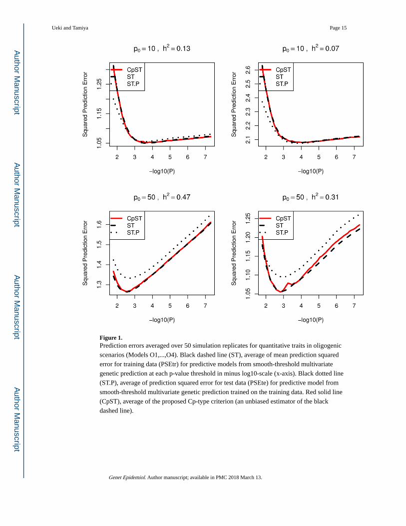
Figure 1. Prediction errors averaged over 50 simulation replicates for quantitative traits in oligogenic
scenarios (Models O1,...,O4). Black dashed line (ST), average of mean prediction squared
error for training data (PSEtr) for predictive models from smooth-threshold multivariate
genetic prediction at each p-value threshold in minus log10-scale (x-axis). Black dotted line
(ST.P), average of prediction squared error for test data (PSEte) for predictive model from
smooth-threshold multivariate genetic prediction trained on the training data. Red solid line
(CpST), average of the proposed Cp-type criterion (an unbiased estimator of the black
dashed line).
Ueki and Tamiya Page 15
Genet Epidemiol. Author manuscript; available in PMC 2018 March 13.
Author M
anuscriptA
uthor Manuscript
Author M
anuscriptA
uthor Manuscript
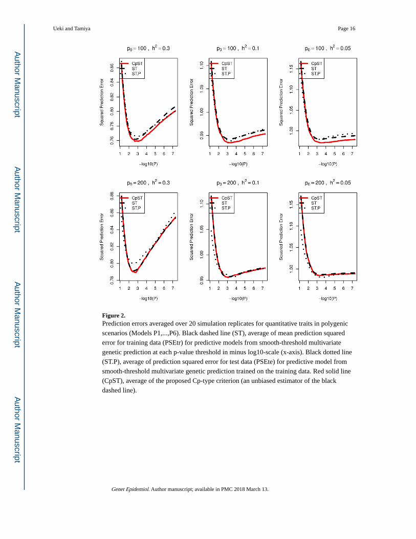
Figure 2. Prediction errors averaged over 20 simulation replicates for quantitative traits in polygenic
scenarios (Models P1,...,P6). Black dashed line (ST), average of mean prediction squared
error for training data (PSEtr) for predictive models from smooth-threshold multivariate
genetic prediction at each p-value threshold in minus log10-scale (x-axis). Black dotted line
(ST.P), average of prediction squared error for test data (PSEte) for predictive model from
smooth-threshold multivariate genetic prediction trained on the training data. Red solid line
(CpST), average of the proposed Cp-type criterion (an unbiased estimator of the black
dashed line).
Ueki and Tamiya Page 16
Genet Epidemiol. Author manuscript; available in PMC 2018 March 13.
Author M
anuscriptA
uthor Manuscript
Author M
anuscriptA
uthor Manuscript
Figure 3. Prediction −2 × loglikelihood averaged over 50 simulation replicates for binary traits in
oligogenic scenarios (O5,...,O8). Black dashed line (ST), average of mean −2 ×
loglikelihood for training data (PSEtr) for predictive models from smooth-threshold
multivariate genetic prediction at each p-value threshold in minus log10-scale (x-axis).
Black dotted line (ST.P), average of prediction −2 × loglikelihood for test data (PSEte) for
predictive model from smooth-threshold multivariate genetic prediction trained on the
training data. Red solid line (CpST), average of the proposed Cp-type criterion (an
approximate unbiased estimator of the black dashed line).
Ueki and Tamiya Page 17
Genet Epidemiol. Author manuscript; available in PMC 2018 March 13.
Author M
anuscriptA
uthor Manuscript
Author M
anuscriptA
uthor Manuscript
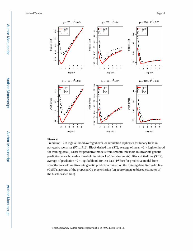
Figure 4. Prediction −2 × loglikelihood averaged over 20 simulation replicates for binary traits in
polygenic scenarios (P7,...,P12). Black dashed line (ST), average of mean −2 × loglikelihood
for training data (PSEtr) for predictive models from smooth-threshold multivariate genetic
prediction at each p-value threshold in minus log10-scale (x-axis). Black dotted line (ST.P),
average of prediction −2 × loglikelihood for test data (PSEte) for predictive model from
smooth-threshold multivariate genetic prediction trained on the training data. Red solid line
(CpST), average of the proposed Cp-type criterion (an approximate unbiased estimator of
the black dashed line).
Ueki and Tamiya Page 18
Genet Epidemiol. Author manuscript; available in PMC 2018 March 13.
Author M
anuscriptA
uthor Manuscript
Author M
anuscriptA
uthor Manuscript
Author M
anuscriptA
uthor Manuscript
Author M
anuscriptA
uthor Manuscript
Ueki and Tamiya Page 19
Tab
le 1
Qua
ntita
tive
trai
ts s
imul
atio
ns, a
vera
ge p
redi
ctiv
e co
rrel
atio
n co
-eff
icie
nt (
PCC
) w
ith s
tand
ard
devi
atio
n in
par
enth
esis
, ave
rage
num
ber
of tr
ue/f
alse
posi
tive
(TP/
FP)
resu
lts f
or th
ree
met
hods
in r
eplic
ates
. ST
MG
P, s
moo
th-t
hres
hold
mul
tivar
iate
gen
etic
pre
dict
ion,
Ene
t, el
astic
net
; GS,
gen
e sc
ore.
The
best
per
form
ing
met
hod
is e
mph
asiz
ed in
bol
d.
p 0h2
STM
GP
Las
soE
net
GC
TA
GS
Olig
ogen
ic s
cena
rios
(n
= 1
000)
100.
13PC
C0.
27 (
0.11
)0.
28 (
0.11
)0.
27 (
0.11
)0.
09 (
0.1)
0.1
(0.0
9)
TP/
FP3/
115
2/46
3/19
4-
4/30
88
100.
07PC
C0.
16 (
0.12
)0.
16 (
0.12
)0.
16 (
0.12
)0.
05 (
0.1)
0.04
(0.
11)
TP/
FP2/
781/
322/
133
-4/
7105
500.
47PC
C0.
55 (
0.1)
0.57
(0.
09)
0.55
(0.
09)
0.27
(0.
09)
0.29
(0.
1)
TP/
FP16
/509
11/1
5119
/816
-20
/348
8
500.
31PC
C0.
18 (
0.21
)0.
17 (
0.21
)0.
17 (
0.2)
0.18
(0.
09)
0.19
(0.
11)
TP/
FP5/
133
3/50
6/26
4-
18/4
373
Poly
geni
c sc
enar
ios
(n =
500
0)
100
0.3
PCC
0.46
(0.
11)
0.48
(0.
11)
0.47
(0.
11)
0.28
(0.
14)
0.31
(0.
1)
TP/
FP29
/904
24/5
0236
/107
3-
36/2
636
100
0.1
PCC
0.23
(0.
1)0.
23 (
0.11
)0.
23 (
0.11
)0.
11 (
0.13
)0.
13 (
0.14
)
TP/
FP12
/257
10/2
1517
/570
-30
/641
3
100
0.05
PCC
0.12
(0.
11)
0.13
(0.
09)
0.13
(0.
11)
0.06
(0.
12)
0.05
(0.
12)
TP/
FP6/
125
5/12
99/
406
-23
/752
1
200
0.3
PCC
0.41
(0.
09)
0.44
(0.
1)0.
43 (
0.1)
0.28
(0.
09)
0.3
(0.0
9)
TP/
FP40
/101
730
/434
52/1
395
-54
/272
6
200
0.1
PCC
0.15
(0.
12)
0.17
(0.
13)
0.18
(0.
12)
0.11
(0.
1)0.
11 (
0.1)
TP/
FP13
/263
8/14
019
/600
-37
/457
7
200
0.05
PCC
0.09
(0.
1)0.
09 (
0.12
)0.
1 (0
.11)
0.06
(0.
11)
0.06
(0.
06)
TP/
FP5/
117
4/10
97/
300
-37
/731
2
Genet Epidemiol. Author manuscript; available in PMC 2018 March 13.
Author M
anuscriptA
uthor Manuscript
Author M
anuscriptA
uthor Manuscript
Ueki and Tamiya Page 20
Tab
le 2
Bin
ary
trai
ts s
imul
atio
ns, a
vera
ge A
UC
with
sta
ndar
d de
viat
ion
in p
aren
thes
is, a
nd a
vera
ge n
umbe
r of
true
/fal
se p
ositi
ve (
TP/
FP)
resu
lts f
or th
ree
met
hods
in r
eplic
ates
. ST
MG
P, s
moo
th-t
hres
hold
mul
tivar
iate
gen
etic
pre
dict
ion;
Ene
t, el
astic
net
; GS,
gen
e sc
ore.
The
bes
t per
form
ing
met
hod
is e
mph
asiz
ed in
bold
.
p 0h2
STM
GP
Las
soE
net
GC
TA
GS
Olig
ogen
ic s
cena
rios
(n
= 1
000)
100.
05A
UC
0.55
(0.
06)
0.55
(0.
06)
0.56
(0.
05)
0.51
(0.
06)
0.52
(0.
06)
TP/
FP2/
991/
238
2/45
1-
4/54
41
100.
11A
UC
0.64
(0.
06)
0.64
(0.
08)
0.64
(0.
07)
0.52
(0.
07)
0.53
(0.
06)
TP/
FP3/
115
2/31
3/64
-5/
6082
500.
04A
UC
0.51
(0.
05)
0.5
(0.0
5)0.
51 (
0.05
)0.
51 (
0.06
)0.
51 (
0.05
)
TP/
FP1/
471/
360
2/68
8-
9/81
19
500.
09A
UC
0.53
(0.
05)
0.52
(0.
05)
0.53
(0.
05)
0.52
(0.
05)
0.52
(0.
04)
TP/
FP2/
111
2/27
33/
407
-13
/917
5
Poly
geni
c sc
enar
ios
(n =
500
0)
100
0.3
AU
C0.
74 (
0.05
)0.
74 (
0.04
)0.
74 (
0.04
)0.
64 (
0.05
)0.
66 (
0.05
)
TP/
FP30
/115
021
/142
29/4
35-
36/2
754
100
0.1
AU
C0.
61 (
0.05
)0.
61 (
0.05
)0.
61 (
0.05
)0.
55 (
0.04
)0.
55 (
0.04
)
TP/
FP15
/432
8/60
13/1
78-
21/1
459
100
0.05
AU
C0.
54 (
0.03
)0.
54 (
0.03
)0.
54 (
0.04
)0.
53 (
0.04
)0.
52 (
0.03
)
TP/
FP7/
285
4/24
87/
680
-17
/395
6
200
0.3
AU
C0.
75 (
0.05
)0.
76 (
0.05
)0.
76 (
0.04
)0.
66 (
0.05
)0.
68 (
0.07
)
TP/
FP53
/174
532
/223
49/6
94-
55/2
341
200
0.1
AU
C0.
58 (
0.03
)0.
59 (
0.04
)0.
59 (
0.04
)0.
55 (
0.03
)0.
55 (
0.04
)
TP/
FP18
/505
9/95
15/2
77-
49/7
276
200
0.05
AU
C0.
54 (
0.03
)0.
53 (
0.03
)0.
54 (
0.03
)0.
52 (
0.03
)0.
53 (
0.04
)
TP/
FP7/
212
7/82
011
/117
8-
39/7
869
Genet Epidemiol. Author manuscript; available in PMC 2018 March 13.
Author M
anuscriptA
uthor Manuscript
Author M
anuscriptA
uthor Manuscript
Ueki and Tamiya Page 21
Tab
le 3
Pred
ictiv
e po
wer
for
AD
NI-
WG
S sa
mpl
es f
or th
ree
kind
s of
phe
noty
pe d
efin
ition
s an
d tw
o co
vari
ate
adju
stm
ents
: (i)
nor
mal
(=
1), M
CI
(=2)
and
AD
(=
3)
(mea
sure
d by
pre
dict
ive
corr
elat
ion
coef
fici
ent (
SD))
, (ii)
nor
mal
(=
1), M
CI
(=2)
and
AD
(=
2) (
mea
sure
d by
AU
C (
SD))
, (iii
) no
rmal
(=
1), M
CI
(=1)
and
AD
(=
2) (
mea
sure
d by
AU
C (
SD))
; (a)
sex
and
age
, (b)
sex
, age
, yea
r of
edu
catio
n (E
DU
) an
d fa
mily
his
tory
(FH
). O
ptP,
opt
imal
p-v
alue
cut
off
by
STM
GP
(−lo
g10
scal
e). N
S, n
umbe
r of
scr
eene
d SN
Vs
by S
TM
GP.
(i)
Cov
aria
tes
STM
GP
GC
TA
GS
Opt
PN
S
(a
)0.
22 (
0.11
)0.
06 (
0.14
)0.
07 (
0.11
)4.
7 (0
.5)
362
(350
)
(b
)0.
24 (
0.12
)−
0.06
(0.
1)0.
05 (
0.1)
4.9
(0.3
)24
7 (1
60)
(ii)
Cov
aria
tes
STM
GP
GC
TA
GS
Opt
PN
S
(a
)0.
61 (
0.05
)0.
54 (
0.09
)0.
51 (
0.09
)4.
8 (0
.4)
143
(104
)
(b
)0.
63 (
0.08
)0.
44 (
0.08
)0.
51 (
0.09
)4.
8 (0
.4)
113
(82)
(iii)
Cov
aria
tes
STM
GP
GC
TA
GS
Opt
PN
S
(a
)0.
60 (
0.15
)0.
51 (
0.17
)0.
52 (
0.18
)3.
5 (0
)35
23 (
309)
(b
)0.
69 (
0.15
)0.
47 (
0.15
)0.
55 (
0.21
)3.
5 (0
)36
01 (
296)
Genet Epidemiol. Author manuscript; available in PMC 2018 March 13.


![Automated hippocampal segmentation in 3D MRI using …adni.loni.usc.edu/adni-publications/Maglietta_2016_pattern analysis.pdfemployed as segmentation tools in [11]. RF uses multiple](https://img.pdfslide.us/doc/110x75/5e62aef5c459b244b608e663/automated-hippocampal-segmentation-in-3d-mri-using-adniloniusceduadni-publicationsmaglietta2016pattern.jpg)