HHS Public Access 1 Scott C Brown Peter Eschbach Li Han

Particle size distributions by transmission electron microscopy: an interlaboratory comparison case study

Stephen B Rice1, Christopher Chan2, Scott C Brown2, Peter Eschbach3, Li Han4, David S Ensor4, Aleksandr B Stefaniak5, John Bonevich6, András E Vladár6, Angela R Hight Walker6, Jiwen Zheng7, Catherine Starnes8, Arnold Stromberg8, Jia Ye9, and Eric A Grulke9

1 Lawrence Murphy, Cabot Corporation, 157 Concord Road, Billerica, MA 01821, USA

2 Dupont Central Research and Development, Experimental Station—Bldg 228, PO Box 80228, Wilmington, DE 19880-0228, USA

3 Hewlett Packard Corporation, OR, USA

4 RTI International, Aerosol Science, Nanotechnology Engineering Technology Unit, 3040 Cornwallis Rd, PO Box 12194, Research Triangle Park, NC 27709, USA

5 National Institute for Occupational Safety and Health, 095 Willowdale Road, Morgantown, WV 26505, USA

6 National Institute of Standards and Technology, 100 Bureau Drive, Stop 8443, Gaithersburg, MD 20899-8443, USA

7 US Food and Drug Administration, Division of Chemistry and Materials Science (DCMS), WO62, Room G102, 10903 New Hampshire Avenue, Silver Spring, MD 20993, USA

8 Statistics Department and Applied Statistics Laboratory, University of Kentucky, Lexington, KY 40506, USA

9 Chemical and Materials Engineering, University of Kentucky, Lexington, KY 40506, USA

Abstract

This paper reports an interlaboratory comparison that evaluated a protocol for measuring and

analysing the particle size distribution of discrete, metallic, spheroidal nanoparticles using

transmission electron microscopy (TEM). The study was focused on automated image capture and

automated particle analysis. NIST RM8012 gold nanoparticles (30 nm nominal diameter) were

measured for area-equivalent diameter distributions by eight laboratories. Statistical analysis was

used to (1) assess the data quality without using size distribution reference models, (2) determine

reference model parameters for different size distribution reference models and non-linear

regression fitting methods and (3) assess the measurement uncertainty of a size distribution

parameter by using its coefficient of variation. The interlaboratory area-equivalent diameter mean,

27.6 nm ± 2.4 nm (computed based on a normal distribution), was quite similar to the area-

equivalent diameter, 27.6 nm, assigned to NIST RM8012. The lognormal reference model was the

preferred choice for these particle size distributions as, for all laboratories, its parameters had

[email protected].

HHS Public AccessAuthor manuscriptMetrologia. Author manuscript; available in PMC 2015 September 08.

Published in final edited form as:Metrologia. 2013 November ; 50(6): 663–678. doi:10.1088/0026-1394/50/6/663.

Author M

anuscriptA

uthor Manuscript

Author M

anuscriptA

uthor Manuscript

lower relative standard errors (RSEs) than the other size distribution reference models tested

(normal, Weibull and Rosin–Rammler–Bennett). The RSEs for the fitted standard deviations were

two orders of magnitude higher than those for the fitted means, suggesting that most of the

parameter estimate errors were associated with estimating the breadth of the distributions. The

coefficients of variation for the interlaboratory statistics also confirmed the lognormal reference

model as the preferred choice. From quasi-linear plots, the typical range for good fits between the

model and cumulative number-based distributions was 1.9 fitted standard deviations less than the

mean to 2.3 fitted standard deviations above the mean. Automated image capture, automated

particle analysis and statistical evaluation of the data and fitting coefficients provide a framework

for assessing nanoparticle size distributions using TEM for image acquisition.

1. Introduction

1.1. Nanoparticle size distributions by transmission electron microscopy

Nanotechnology research is accelerating innovation. For example, the number of

nanoparticle patents has an exponential growth rate of >30% in recent years. Nano-objects

are materials with one, two or three external dimensions on the nanoscale, nominally

ranging from 1 nm to 100 nm [1]. Nanoparticles, which have all three external dimensions

on the nanoscale, have performance properties that often depend on their physico-chemical

characteristics, i.e. size, shape, surface structure and texture. For example, catalytic

properties of nanoparticles usually depend on their crystal structures, size distributions and

exposed surfaces, edges and corners. The growth rates of different crystallographic surfaces

can vary, leading to asymmetric particles [2]. Toxicity can be affected by nanoparticle size

[3], which makes this an important metric for risk assessment [4, 5]. Stakeholders in

nanoparticle characterization include industry, academics, government agencies (and

particularly, regulatory agencies), and the general public through non-governmental

organizations.

There are a wide variety of analytical methods for particle size measurements, including

electron microscopy, dynamic light scattering [6], centrifugal liquid sedimentation, small-

angle x-ray scattering, field flow fractionation, particle tracking analysis, atomic force

microscopy [7] and x-ray diffraction [8]. These methods are based on different measurands,

and a comparison between methods should be made with care. Many of the measurement

methods for particle sizes on the nanoscale have focused on assessing an average particle

size for the sample. Performance properties of nanoparticles often depend on size and shape

and few particle size distributions of commercial products are monomodal and narrow in

range. In fact, the nanoparticle size distribution is important to product performance in

applications, in the environment, and for health and safety and for regulations. Transmission

electron microscopy (TEM) methods provide two-dimensional images of nanoparticles;

these images can be used to produce number-based size distributions.

1.2. Analysis and reporting of size distributions

Because we are interested in more than a single point representation of the sample size, we

compared appropriate reference distributions, such as the normal, lognormal and Weibull

distributions, with particle size distribution data. TEM particle size data were converted

Rice et al. Page 2

Metrologia. Author manuscript; available in PMC 2015 September 08.

Author M

anuscriptA

uthor Manuscript

Author M

anuscriptA

uthor Manuscript

directly to cumulative number-based distributions. This information is useful for both

nanoparticle applications, for which the surface properties may be distinctly different below

a specific length scale, and regulatory requirements, for which the fraction of particles below

a length scale of 100 nm would be related to whether the sample is on the nanoscale. Size

distribution reference models generally have two parameters, representing the size and the

shape of the distribution. For the normal distribution, these would be the sample mean and

the sample standard deviation. The number of particles needed for high-accuracy estimates

of the average diameter is known to depend on the spread of the particle size distribution [9].

An important step in the process is visualizing the fitted model prediction relative to the

actual data. This step helped us answer the following question: where does the model

deviate from the data, i.e. over what diameter range do we know the distribution well? This

has relevance for the application and regulatory communities. Because TEM can be a costly

method, automated image capture, particle analysis and statistical assessment were

preferred.

1.3. Metrology checklist and term definitions

A metrology checklist [10], established by ISO/TC 229, was used to assess and design the

protocol (appendix A). There are a variety of reference materials for characterizing

nanoparticle size (see [11] for lists of reference materials [12] and their sources). RM8012, a

suspension of discrete, spheroidal, gold nanoparticles with a nominal size of 30 nm (NIST),

was used in this study to facilitate sample preparation, image capture, particle analysis and

statistical assessment of measurement uncertainty. Appendix B provides definitions of

statistical, measurands and metrology terms used in this study.

1.4. Protocol objectives

This case study is intended to provide a scientific foundation for an International

Organization for Standardization (ISO; www.iso.org) standard for the measurement of

particle size distributions on the nanoscale by TEM. The committee, ISO/TC 229

Nanotechnologies, was established in 2005, and now has 34 national member bodies, about

40 liaison members (other ISO TCs or international organizations), along with 11 observers.

The authors of this study are members of the US Technical Advisory Group (TAG) to TC

229. Standards developed by ISO/TC 229 are intended to improve commerce and facilitate

communications among buyers, sellers and regulators of raw and intermediate materials.

The case study protocol for 30 nm gold nanoparticles was based on a National Institute for

Occupational Safety and Health (NIOSH) internal interlaboratory comparison [13, 14] and a

generic protocol from the UK National Physical Laboratory [15]. Discrete, spheroidal

nanoparticles represent one of the less-complex nanoparticle morphologies; measurands of

this sample should have relatively high reproducibility, and fitted parameters modelling the

distributions should have low relative standard errors (RSEs). There are many TEM

instruments, and sample preparation techniques are often tuned by each operator for their

system. Typically, TEM sample preparation is a major contributor to measurement

uncertainty. Sample preparation was not assessed in this case study. Sample mounting and

dilution guidance from previous studies of this reference material was used by one lab to

Rice et al. Page 3


Author M

anuscriptA

uthor Manuscript

Author M

anuscriptA

uthor Manuscript

http://www.iso.org

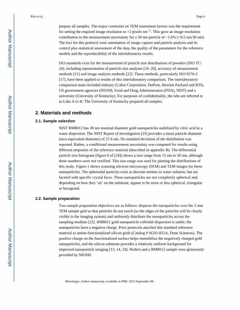
prepare all samples. The major constraint on TEM instrument factors was the requirement

for setting the required image resolution to >2 pixels nm−1. This gave an image resolution

contribution to the measurement uncertainty for a 30 nm particle of ~1.6% (<0.5 nm/30 nm).

The foci for this protocol were automation of image capture and particle analysis and its

control plus statistical assessment of the data, the quality of the parameters for the reference

models and the reproducibility of the interlaboratory results.

ISO standards exist for the measurement of particle size distributions of powders (ISO TC/

24), including representation of particle size analyses [16–20], accuracy of measurement

methods [21] and image analysis methods [22]. These methods, particularly ISO 9276-3

[17], have been applied to results of this interlaboratory comparison. The interlaboratory

comparison team included industry (Cabot Corporation, DuPont, Hewlett Packard and RTI),

US government agencies (NIOSH, Food and Drug Administration (FDA), NIST) and a

university (University of Kentucky). For purposes of confidentiality, the labs are referred to

as Labs A to H. The University of Kentucky prepared all samples.

2. Materials and methods

2.1. Sample selection

NIST RM8012 has 30 nm nominal diameter gold nanoparticles stabilized by citric acid in a

water dispersion. The NIST Report of Investigation [23] provides a mean particle diameter

(area-equivalent diameter) of 27.6 nm. No standard deviation of the distribution was

reported. Rather, a conditional measurement uncertainty was computed for results using

different ampoules of the reference material (described in appendix B). The differential

particle size histogram (figure 6 of [24]) shows a size range from 15 nm to 50 nm, although

these numbers were not certified. This size range was used for plotting the distributions of

this study. Figure 1 shows scanning electron microscopy (SEM) and TEM images for these

nanoparticles. The spheroidal particles exist as discrete entities in water solution, but are

faceted with specific crystal faces. These nanoparticles are not completely spherical and,

depending on how they ‘sit’ on the substrate, appear to be more or less spherical, triangular

or hexagonal.

2.2. Sample preparation

Two sample preparation objectives are as follows: disperse the nanoparticles over the 3 mm

TEM sample grid so that particles do not touch (so the edges of the particles will be clearly

visible in the imaging system) and uniformly distribute the nanoparticles across the

sampling medium [22]. RM8012 gold nanoparticle colloidal dispersion is stable; the

nanoparticles have a negative charge. Prior protocols attached this standard reference

material to amine-functionalized silicon grids (Catalog # SG01-051A, Dune Sciences). The

positive charge on the functionalized surface helps immobilize the negatively charged gold

nanoparticles, and the silicon substrate provides a relatively uniform background for

improved nanoparticle imaging [13, 14, 24]. Wafers and a RM8012 sample were generously

provided by NIOSH.

Rice et al. Page 4


Author M

anuscriptA

uthor Manuscript

Author M

anuscriptA

uthor Manuscript

The typical time required to receive the sample, acquire over 500 data points, analyse the

data with ImageJ and assemble the frame-wise data into a master table for analysis exceeded

20 h. Each lab received one grid; no grids were shared between laboratories.

2.3. Instrument factors

ISO 13322-1:2004 [22] provides guidance on electron microscope operating conditions for

particle size imaging and a measurement uncertainty analysis specifically for lognormal

distributions, which would be the most common reference model for nanoparticle

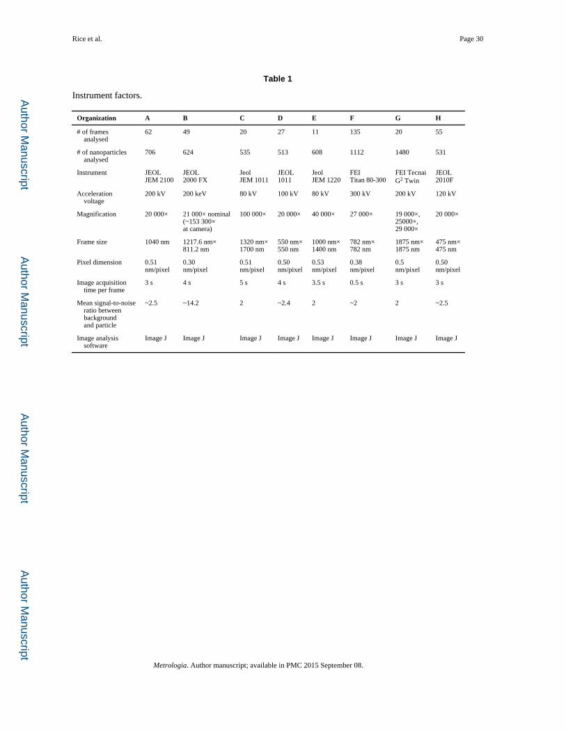
distributions. Table 1 shows the instrument factors of each lab. Specific guidance was as

follows [22]:

• set the accelerating voltage according to the material to be measured (120 kV);

• select the sample working distance specified by the electron microscope

manufacturer for high-resolution imaging;

• mount the sample flat on the specimen holder with the stage tilt set to zero;

• switch off the dynamic focus and tilt correction;

• align the instrument according to the manufacturer’s procedures;

• select operating conditions to minimize drift.

While no SEM instruments were used in this study for particle size determination, it is

notable that a recent good practice guide [15] provides some guidance on selection of

instrument parameters for use with this type of instrument for particle sizing.

Calibration—Since TEMs have wide ranges of magnification and many operating modes,

the actual magnification at any given instrument settings may differ from the indicated

magnification by up to 10%. Calibration of the instrument to a known length scale under

optical conditions similar to those used for analysis is preferred. Standards should be run

near the time of the study to provide verification of correct instrument operation within

manufacturer specifications and to validate measurement procedures. Typical examples are

given in a good practice guide ([15, chapter 4]).

2.4. Image acquisition

Each participating lab used the loading procedure specific for their instrument to mount the

TEM grid in the system. The loading procedure was to minimize the eucentric height

adjustment required. The images were to be of sufficient quality such that individual

particles can be resolved and their dimensions measured. Each lab analysed one wafer,

measured at least 500 particles, and reported the results to the team. The specific instructions

were the following.

• Acquire images that have histograms centred and wide enough to cover at least

80% of the possible grey levels.

• Select a magnification/image resolution combination that will provide a minimum

of two pixels/nm, i.e. >2 pixel nm−1 or <0.5 nm/pixel.

Rice et al. Page 5


Author M

anuscriptA

uthor Manuscript

Author M

anuscriptA

uthor Manuscript

• Ensure that a scale bar is visible in each digital image/frame.

• Do not exclude irregularly shaped particles or particles with sharp corners.

• Do not report data for any touching particles (note: overlapping particles can rest

on one another, reducing their projected 2D area in a top-down view).

• Do not report data for any particles that appear cut by the frame (note: for the case

in which there is a difference in particle diameters greater than an order of

magnitude, it may be necessary to establish a frame, divide it via a grid pattern, and

measure large particles at a lower magnification. The protocol did not address this

issue).

• Count and report at least 500 particles in frames that are well spaced across the

sample (note: the number of particles measured directly affects the measurement

uncertainty of the sample mean and standard deviation. In general, the user will

select precisions for the sample mean and standard deviation, and then estimate

how many particles might be needed. There is guidance on how the sample mean is

affected by the sample size [9, 25–28], but less guidance on the effects of sample

size on the sample standard deviation).

• For all selected particles in each frame, report the particle number, the frame

number and all measurand data.

• Save images as lossless (like tagged image file format, tiff or dmc) image file type.

Do not save images as lossy image file type, like jpg.

The area-equivalent average diameters of all reported particles were used to generate

number-based, cumulative particle size distributions.

2.5. Particle analysis

Since a large number of nanoparticles are needed for a high-quality particle size distribution,

the work will be facilitated when image analysis software is used. Both commercial and

open source software are available. For a typical sample, an appropriate reference model for

the data may not be known, the data may not be monomodal, and the sample may be

contaminated with nanoparticles of different sizes and shapes. Multiple models might need

to be compared with the data and multiple measurands might be needed to help screen for

the desired nanoparticles. Therefore, we have used a more general analysis approach that

estimates the sample mean and standard deviation from a non-linear fit of the reference

model to sample population data. The minimum number of particles for analysis was set at

500 for each lab, based on the experience from prior studies.

This protocol assumed that all images were taken in digital format. ImageJ, open source

software with a suite of analysis routines (http://rsbweb.nih.gov/ij/download.html), was used

by all laboratories for particle analysis. The procedure steps were as follows.

• Create working copies of all images/frames (preserve the original unmodified

images).

• Open ImageJ and open the frame file.

Rice et al. Page 6


Author M

anuscriptA

uthor Manuscript

Author M

anuscriptA

uthor Manuscript

http://rsbweb.nih.gov/ij/download.html

• Set the measurement scale using the scale bar or another measurement of pixel size,

returning to the original scale prior to continuing.

• Crop the image to remove scale bars and other image artefacts that might affect

contrast or particle analysis.

• Check and correct brightness and contrast to ensure that all images have histograms

centred and wide enough to cover at least 80% of the possible grey levels.

• The thresholding operation may result in frame files with single pixel artefacts or

poor image quality, e.g. rough particles or uneven background due to non-uniform

electron beam illumination. In the case of the former, apply the despeckle and

erode/dilate processes to remove these artefacts and save the changes. In the case of

poor image quality, the operator could clean up the edges of particles or correct for

uneven background by applying special filters. Assess the image transformation

and save changes.

• Touching particles should not be addressed by using automated separation

algorithms (Watershed, in the case of ImageJ). Rather, all particle analyses should

be recorded, and touching particles should be removed manually from the

spreadsheet of the results.

• Select the measurands (such as area, shape descriptors, Feret’s diameter). Note:

several size and shape descriptors will help identify imaging and measurement

issues as well as assist with the characterization of the sample.

• Analyse the particles (ImageJ specific settings should include the following: show

outlines, display results, include holes and exclude on edges).

• Save each image file that shows particle outlines and their number sequence

(filename.tif) and the spreadsheet (Results.xls), which reports all measurand values,

the particle number and the frame number associated with each particle.

2.6. Data analysis

There are three major applications for statistical analysis of particle size data: assessment of

data robustness, fitting reference models to the size distributions and assessment of

measurement uncertainty.

2.6.1. Statistical assessment of data—Analysis of variance (ANOVA) was used to

assess the intra-laboratory repeatability (variation with one operator and one instrument;

section 2.20 of [29]) and interlaboratory reproducibility (variation of measurements with the

same process done with different instruments and different operators; section 2.24 of [29]).

At the specified resolution (>2 pixels nm−1), there were usually a small number of

nanoparticles in any given view frame for most labs. It is not likely that reasonable estimates

for the sample size mean and standard deviation can be obtained from one frame. Therefore,

one-way ANOVA was used to test the null hypothesis (see the definition in appendix B) that

all of the frames within one lab had the same mean area-equivalent diameter (repeatability).

Also, ANOVA with the frames treated as a random effect nested within labs was used to

investigate the null hypothesis that the mean area-equivalent diameter among laboratories

Rice et al. Page 7


Author M

anuscriptA

uthor Manuscript

Author M

anuscriptA

uthor Manuscript

was the same (reproducibility). Finally, since RM8012 was investigated for its mean area-

equivalent diameter, the bias (or trueness; appendix B and sections 2.14, 2.14 of [29]) of the

reported area-equivalent diameters can be estimated.

For intra-laboratory repeatability, the objective, metric and software were as follows.

Objective: assess whether all frames within a selected lab are best represented by the same

mean.

• Null hypothesis: for each lab, all frames have the same mean.

• Alternative hypothesis: for each lab, not all frames have the same mean.

Metric: if the p-value <0.05, then we reject the null hypothesis and conclude that at least two

frames reported by that lab have different averages.

Software: SAS v9.3, the GLM procedure (http://support.sas.com/documentation/cdl/en/

statug/62962/HTML/default/viewer.htm#glm_toc.htm). A program is available for

interlaboratory comparison users to perform this test on data matrices imported from an

Excel spreadsheet.

For interlaboratory reproducibility, the objective, metric and software were as follows.

Objective: assess whether all labs are best represented by the same mean.

• Null hypothesis: all labs have the same mean.

• Alternative hypothesis: not all labs have the same mean.

Metric: if the p-value <0.05, then we reject the null hypothesis and conclude that at least two

labs have different averages.

Software: SAS v9.3, the MIXED procedure (http://support.sas.com/documentation/cdl/en/

statug/63962/HTML/default/viewer.htm#mixed_toc.htm).

2.6.2. Fitting reference models to data—Three reference models are commonly fitted

to cumulative particle size distribution data: lognormal, Rosin–Rammler–Bennett and

Weibull. These three, plus the normal distribution, were compared with the cumulative

frequency data generated in this case study. In all cases, two parameter models were used.

Differential probability distributions were not used as information is lost when the data are

binned, often obscuring the details near the ends of the distributions.

Three different visualization methods [17] were used to optimize the parameter estimates for

cumulative distribution data: (1) minimizing the variance between the data and reference

model, (2) setting the residual deviations between the data and reference model to zero and

(3) transforming the three reference models into linear functions (quasi-linear regression). A

commercial non-linear regression package, SYSTAT® software (version 10.1), was used to

optimize parameters for each data set.

The software provided the R2 value for the optimized fit, the parameter estimates (for

example, the mean, x(fit), and standard variation, s(fit)), and the standard errors of the

Rice et al. Page 8


Author M

anuscriptA

uthor Manuscript

Author M

anuscriptA

uthor Manuscript

http://support.sas.com/documentation/cdl/en/statug/62962/HTML/default/viewer.htm#glm_toc.htm

http://support.sas.com/documentation/cdl/en/statug/62962/HTML/default/viewer.htm#glm_toc.htm

http://support.sas.com/documentation/cdl/en/statug/63962/HTML/default/viewer.htm#mixed_toc.htm

http://support.sas.com/documentation/cdl/en/statug/63962/HTML/default/viewer.htm#mixed_toc.htm

parameter estimates (for example, SEx(fit) and SEs(fit)). The mean and the standard deviation

of the model are descriptive statistics. The standard error of a descriptive statistics describes

the expected bounds for a random sampling process; it describes how close the sample

statistic (the mean or standard deviation) is to those of the population. The standard errors

were determined using Wald confidence intervals, which are appropriate when there is little

correlation between the fitted parameters, i.e. the mean and the standard deviation (this is the

case for all of our data). The ratio of the standard error to the estimate is the RSE. The RSE

decreases as the number of particles increases; smaller RSE values indicate that the estimate

of the parameter for the sample is closer to that of the whole population. The RSE can be

used as a measure of quality for fitted parameters, facilitating the comparisons of different

reference models, different measurands and different fitting methods.

For each parameter and its associated statistics, it is possible to construct a ‘grand’ statistic

for the interlaboratory study. For example, the fitted lognormal means that each lab will

have a grand mean and a grand standard deviation. The ratio of the grand standard deviation

to the grand mean is the coefficient of variation for that parameter or statistic (for example,

ĉv,x(fit) and ĉv,s(fit)). The coefficient of variation, a parameter’s standard error divided by its

estimate, is also a type A component of the measurement uncertainty (section 2.26 of [29])

and related to the reproducibility of the data. The definitions for these statistical tools are

given in appendix B.

2.6.3. Assessment of measurement uncertainty—Standards organizations require

statements on measurement uncertainty. There are differences between CEN (Comité

Européen de Normalisation), ISO and ASTM (American Society for Testing and Materials)

approaches [30], although all of these report pooled uncertainties. ASTM uses precision and

bias estimates (ASTM E456), which generally qualifies the test method. ISO Guide to the

Expression of Uncertainty in Measurement (GUM) [31] describes top-down and bottom-up

approaches. The top-down approach, based on repeated testing and the statistical evaluation

of the results, is used often in chemistry (see ISO 5725). The bottom-up approach is more

often (but not only) used in physics. This approach identifies all relevant measurement

parameters, identifies all sources of uncertainties in the test, quantifies each source of

uncertainty with a probability distribution, calculates the combined (pooled) standard

uncertainty, and estimates the expanded uncertainty at the 95% confidence interval. Some

references provide great detail on measurement uncertainty for measurement of particle size

alone [9, 25–28]. We have followed the more general approach of Braun et al [6].

Measurement uncertainty: For the area-equivalent diameter, elements of the pooled

measurement uncertainty, (uc(x)), could include the interlaboratory reproducibility, (u(ir));

the trueness, (u(t)); and the image resolution error, (u(c)). The image resolution error

depends on particle size, ranging from 3.3% to 1.7% to 1% for particle sizes of 15 nm, 30

nm and 50 nm.

Rice et al. Page 9


Author M

anuscriptA

uthor Manuscript

Author M

anuscriptA

uthor Manuscript

For the normal distributions, we have the information needed to compute each of these

components for the sample mean. However, the lognormal mean of RM8012 has not been

reported or certified, so only the interlaboratory reproducibility and the image resolution

error can be computed.

3. Results and discussion

3.1. Sample preparation and instrument factors

Although each laboratory used a different TEM instrument, the sample grids were suitable

for each one. Sample preparation, a known element of variability for TEM analysis, was not

varied in this study. RM8012 is known to have discrete, non-aggregated gold nanoparticles

in its suspension medium. This is confirmed by its Report of Investigation, in which the

average particle size by dynamic light scattering is essentially the same as the size by TEM.

In general, the gold nanoparticles were well separated on the functionalized silicon TEM

grid surfaces, but a number of touching particles were observed on all grids. There are at

least two mechanisms by which this could occur: agglomeration, which is a general

phenomenon for colloidal particles in solution and increases with particle concentrations,

and random deposition of one nanoparticle near another. Touching nanoparticles were

assumed to be agglomerated. For Laboratory H, a total of 672 nanoparticles were imaged.

Of these, there were 530 discrete nanoparticles. Fifty-one dimer, 11 trimer and one septamer

nano-objects were judged to be touching and were not counted, i.e. only 79% of the imaged

nanoparticles could be used directly for the automated particle analysis. It is likely that the

identification of touching particles could be automated by using shape factor or aspect ratio

measurands, but this was not addressed in this interlaboratory comparison.

One lab reported a calibration error, which occurred when two different magnifications were

used for particle imaging (one of these magnifications had not been properly calibrated).

This type of error was easily detected by the ANOVA analysis of frame-to-frame particle

diameter means. In general, the labs could achieve good contrast between nanoparticles and

the background, and the sample preparation method [13] gave a reasonable number of

discrete, non-touching particles on the grids.

3.2. Automated particle analysis via ImageJ

One laboratory reported thresholding problems that resulted in a number of small particle

artefacts being reported. This was detected by reviewing the cumulative particle size

distribution of all the data; about 5% of the ‘particles’ were less than 6 nm, which was

known not to be characteristic of this reference material. The issue was corrected by redoing

the thresholding and ensuring that the despeckle and erode/dilate steps were used. The

effects of the erode/dilate step can be checked directly during the particle analysis process.

The artefacts also could be removed manually, but this would reduce the benefits of

automated analyses.

Touching particles were not analysed in this interlaboratory comparison, although ImageJ

has a tool to do so (Watershed). The Watershed tool separates touching particles by inserting

a linear boundary at the ‘necks’ between particles. This approach tends to reduce the total

area attributed to each particle and to lower the average area-equivalent diameter reported

Rice et al. Page 10


Author M

anuscriptA

uthor Manuscript

Author M

anuscriptA

uthor Manuscript

for the sample. Figure 2 shows residual deviations and quantile plots for the analysis of non-

touching and touching particles reported by Lab E (the maximum Feret diameter was used

as the measurand for these plots). The Watershed algorithm data have larger residual

deviations than the non-touching particle data (figure 2(a)). On a quantile plot, the size

distribution for the Watershed algorithm data is narrower and the mean value of the

distribution is shifted to a lower value (figure 2(b)). The use of this algorithm could

introduce a consistent bias into the sample mean data.

Other factors affecting particle analysis. Even with discrete, spheroidal particles and a good

sample preparation method, the results of the automated particle size analysis can require

additional operator review. Typical analysis problems were thresholding inconsistency and

artefacts created by the inclusion of scale bars in the analysed images. Since gold

nanoparticles are faceted, crystalline solids, different cross-sectional shapes can be present

in the images and very few particles have shape factors near one (representing a circular

cross-section). Although area-equivalent diameter was the preferred measurand for this

study (particularly since this was the measurand investigated for RM8012), other

measurands that relate to nanoparticle shape provide important information about the

sample. These include the minimum and maximum Feret diameters, and the shape factor.

For more complex shapes, additional measurands should be considered [20].

The protocol used for the US TAG interlaboratory comparison on gold nanoparticles

provided no guidance for post-processing review of the raw data from the automated image

capture and particle analysis process. Interlaboratory comparisons of the data showed that

there were differences in the ranges of particle sizes reported as well as the cumulative

particle size distributions. These differences appeared to be due to differences in how

operators treated the data and/or set thresholding parameters.

3.3. Data analysis

3.3.1. Assessment of data quality—Statistical methods used to assess data precision

and accuracy assume homogeneous variance and normally distributed residuals.

Intra-laboratory assessments: The one-way ANOVA test provides a rapid way to assess

whether the data in all frames within a lab are best represented by the same mean. If the null

hypothesis is not rejected, we have more confidence in the data. If the null hypothesis is

rejected, the particle data (images plus measurand results) can be reviewed to determine

whether any artefacts or unusual particles exist in any frame with a mean not equal to the lab

grand mean. Therefore, intra-laboratory statistical assessment can help identify the

following: (1) repeatability, (2) particles that may be outside the expected range for the

distribution, (3) frames with dissimilar mean particle sizes, (4) calibration errors at different

magnification levels, (5) thresholding to eliminate small ‘ghost’ particles, (6) thresholding to

eliminate large particles, (7) touching particles measured as one particle, and others.

Any particles added to or removed from the data set would need to be justified on technical

grounds. We prefer not to use traditional outlier tests to identify particles that appear to be

outside the distribution—we are trying to determine its true ‘breadth’. In addition, showing

the data range and mean for each frame can trigger reviews even when the frame mean may

Rice et al. Page 11


Author M

anuscriptA

uthor Manuscript

Author M

anuscriptA

uthor Manuscript

be similar (an unusually large and an unusually small particle might offset each other, for

example). The variation in the sample means provides an indication of the intra-laboratory

repeatability.

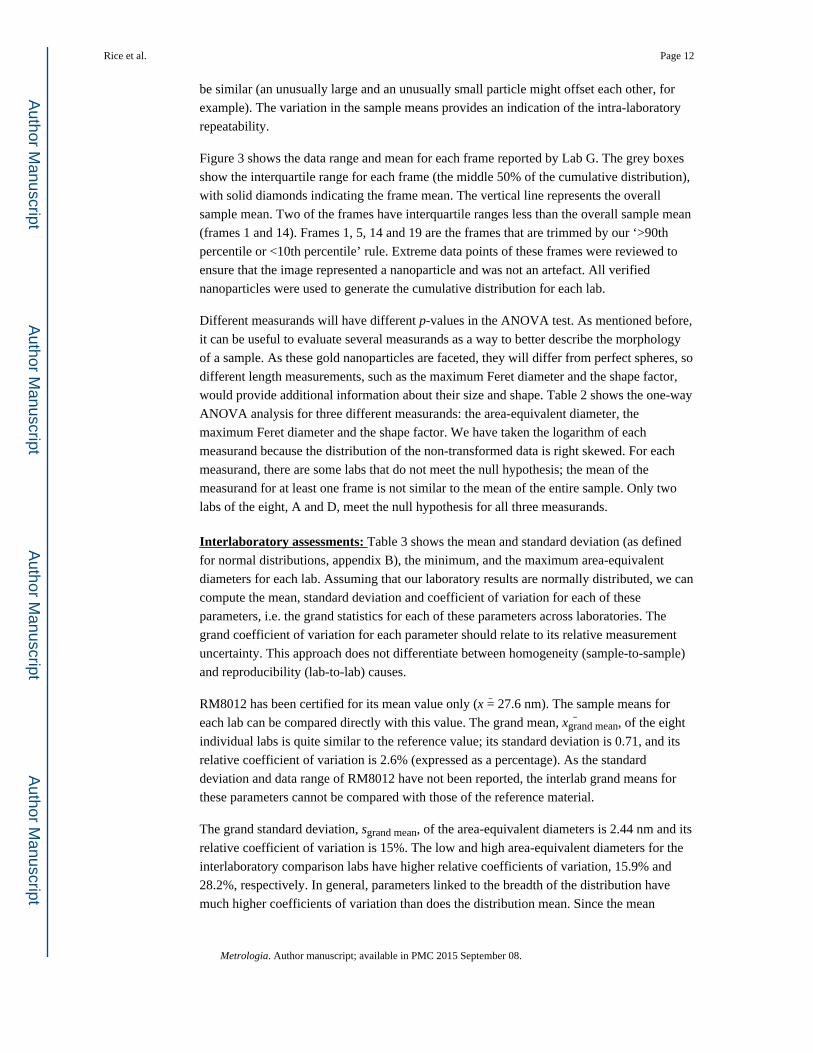
Figure 3 shows the data range and mean for each frame reported by Lab G. The grey boxes

show the interquartile range for each frame (the middle 50% of the cumulative distribution),

with solid diamonds indicating the frame mean. The vertical line represents the overall

sample mean. Two of the frames have interquartile ranges less than the overall sample mean

(frames 1 and 14). Frames 1, 5, 14 and 19 are the frames that are trimmed by our ‘>90th

percentile or <10th percentile’ rule. Extreme data points of these frames were reviewed to

ensure that the image represented a nanoparticle and was not an artefact. All verified

nanoparticles were used to generate the cumulative distribution for each lab.

Different measurands will have different p-values in the ANOVA test. As mentioned before,

it can be useful to evaluate several measurands as a way to better describe the morphology

of a sample. As these gold nanoparticles are faceted, they will differ from perfect spheres, so

different length measurements, such as the maximum Feret diameter and the shape factor,

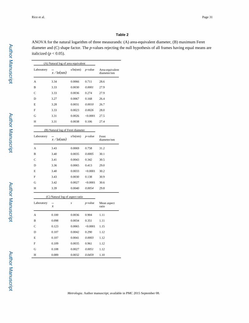
would provide additional information about their size and shape. Table 2 shows the one-way

ANOVA analysis for three different measurands: the area-equivalent diameter, the

maximum Feret diameter and the shape factor. We have taken the logarithm of each

measurand because the distribution of the non-transformed data is right skewed. For each

measurand, there are some labs that do not meet the null hypothesis; the mean of the

measurand for at least one frame is not similar to the mean of the entire sample. Only two

labs of the eight, A and D, meet the null hypothesis for all three measurands.

Interlaboratory assessments: Table 3 shows the mean and standard deviation (as defined

for normal distributions, appendix B), the minimum, and the maximum area-equivalent

diameters for each lab. Assuming that our laboratory results are normally distributed, we can

compute the mean, standard deviation and coefficient of variation for each of these

parameters, i.e. the grand statistics for each of these parameters across laboratories. The

grand coefficient of variation for each parameter should relate to its relative measurement

uncertainty. This approach does not differentiate between homogeneity (sample-to-sample)

and reproducibility (lab-to-lab) causes.

RM8012 has been certified for its mean value only (x = 27.6 nm). The sample means for

each lab can be compared directly with this value. The grand mean, xgrand mean, of the eight

individual labs is quite similar to the reference value; its standard deviation is 0.71, and its

relative coefficient of variation is 2.6% (expressed as a percentage). As the standard

deviation and data range of RM8012 have not been reported, the interlab grand means for

these parameters cannot be compared with those of the reference material.

The grand standard deviation, sgrand mean, of the area-equivalent diameters is 2.44 nm and its

relative coefficient of variation is 15%. The low and high area-equivalent diameters for the

interlaboratory comparison labs have higher relative coefficients of variation, 15.9% and

28.2%, respectively. In general, parameters linked to the breadth of the distribution have

much higher coefficients of variation than does the distribution mean. Since the mean

Rice et al. Page 12


Author M

anuscriptA

uthor Manuscript

Author M

anuscriptA

uthor Manuscript

diameter is reported for RM8012, we can compute the bias using the definition provided in

appendix B. For m = x (the mean of the sample or reference material), the bias is defined as

where Δm = |cm − ccrm| is the absolute difference between the mean measured value and the

certified value.

Table 4 shows the Δm values for each lab. The relative bias for the mean of the

interlaboratory comparison study was 2%.

The interlaboratory assessment used a model with frames nested within labs to identify

differences between pairwise laboratories. Similarly to the intra-laboratory assessment, the

null hypothesis is that every lab has the same mean. Results from the ANOVA test can vary

depending on the measurand. For the area-equivalent diameter measurand, the frame-to-

frame (nested) ANOVA analyses gave similar results when using either the area-equivalent

diameter (corresponding to the normal distribution) or the log transformed measurand

(corresponding to the lognormal distribution). For most lab pairs, the null hypothesis was

rejected; only 4 of 28 pairs fail to reject the null hypothesis. For this comparison, frames

with means less than the 10th percentile or greater than the 90th percentile were excluded,

i.e. data that might be questionable were not considered. This suggests that the lab means

are, in general, different from each other, possibly related to the use of different instruments

and different operators.

3.3.2. Fitting reference models to data—The visual comparison of the data to a

reference model is valuable in selecting which models are appropriate. Figure 4 shows a

cumulative distribution plot of the Rosin–Rammler–Bennett model applied to the shape

factor data of lab H. The equation is shown in the figure; the fitting parameters were selected

to minimize the variance between the model and the data. In general, the model (red curve)

tracks directly through the data except at high values. There are more nanoparticles with

high shape factors than predicted by the model; in this data set, the highest shape factor was

~1.7 and a significant fraction of the nanoparticles had shape factors greater than 1.2. The

median value for the shape factor is 1.07, indicating that the gold nanoparticles are not

perfectly spherical.

Selecting the reference model (measurand = area−equivalent diameter). The lognormal

distribution is the preferred choice for the particle size distribution data in this

interlaboratory comparison as its fitted parameters have lower coefficients of variation than

other reference models. Table 5 reports the parameter estimates, their standard errors, and

the RSEs for the normal and lognormal reference models applied to the data of each lab. The

quality of the fit can be assessed, in part, by comparing the RSE for the parameter estimates

of the two reference models. The RSE grand mean for the lognormal model is one-fourth

that of the RSE grand mean for the normal model. The RSE grand standard deviation for the

lognormal model is about 30% smaller than that of the normal model. The R2 values for

Rice et al. Page 13


Author M

anuscriptA

uthor Manuscript

Author M

anuscriptA

uthor Manuscript

both reference models are close to one and provide little differentiation. The Weibull

distribution was also fitted to these data. It had lower R2 values, higher RSE values, and a

poor fit visually to the cumulative distributions, particularly at the lower particle sizes.

The standard error of a statistic is expected to decrease as the number of data points

increases (SEx ~ 1/√n). As shown in figure 5, the RSEs of the fitted lognormal mean and

standard deviation show an inverse trend to the number of particles measured. The R2 values

of power law correlations for these data RSEs are not high, likely reflecting other factors

associated with the different laboratories.

The coefficient of variation represents the standard deviation of a statistic, and can be used

to compare reference model choices across the interlaboratory study (using the ‘grand mean’

approach). For normal and lognormal distributions, the mean and standard deviation can be

computed both from the standard definitions and the non-linear regression approach (fitted

parameters). Table 6 shows these data for these four cases (two reference models with two

estimation methods). The two coefficients of variation for the fitted parameters (mean and

standard deviation) need to be considered together in making the decision for a reference

model. For the fitted parameters, the coefficient of variation for the lognormal mean is much

smaller than the coefficient of variation for the normal mean, while the coefficients of

variation for the related standard deviations are similar. Therefore, the lognormal reference

model appears to be the better choice when non-linear regression is used. When the standard

definitions for mean and standard deviation are used, the coefficients of variation for the

respective grand means are similar while the coefficient of variation for the standard

deviation of the lognormal reference model is lower than that for the normal reference

model. In this case, the shape of the distribution appears to be better described by the

lognormal model.

Selecting measurands—In this study, the preferred measurand is the area-equivalent

diameter, primarily because the sample itself has been well studied with respect to Da–e.

With more complex morphologies, the choice of key measurands may not always be guided

by the application. For example, nanoparticle shape might be characterized either by the

shape factor or circularity; the choice might be made based on the data quality. Or, different

image processing algorithms might give data of different quality. As discussed in the

previous section, ANOVA tests can be used to identify frame-to-frame similarities of

measurand means. This distribution-independent approach provides some guidance on

which measurands are well known.

A comparison of coefficient of variation values for the area-equivalent and maximum Feret

diameters showed no statistically significant difference between these measurands. The R2

values for the non-linear regression fits were both 0.998. The coefficients of variation for the

means and standard deviations of these measurands were similar, and both values were

within one standard deviation of each other. Therefore, the selection of either would provide

a similar measurement uncertainty for the distribution fit.

Selecting the fitting method—Three fitting methods are described in ISO 9276-3 [17].

Figure 6 compares fitted data for two labs that did not reject the null hypothesis for similar

Rice et al. Page 14


Author M

anuscriptA

uthor Manuscript

Author M

anuscriptA

uthor Manuscript

frame-to-frame means (Labs B and F, table 5). The comparison included the ANOVA

frame-to-frame assessment (boxplot), a cumulative frequency plot, a residual deviation plot

and a quasi-linear regression (quantile) plot. For Lab B, the ANOVA boxplot (A1) shows

relatively uniform distribution of data around the mean diameter (computed using the

standard definition; solid vertical line). The cumulative distribution plot (a2) shows that the

model (solid curve) tracks the data well up to 90% of the sample, then underestimates the

fraction of large particles. The residual deviation plot (a3) shows systematic deviations of

the data from the model. The analysis of this effect is beyond the scope of this work. The

quantile plot (a4) shows that the model tracks the data reasonably well between −2 and +2

standard deviations from the mean (as shown on the Y -axis). Above and below these levels,

there are systematic deviations.

Lab F had the lowest coefficients of variation for its parameters. The boxplot for Lab F (b1)

shows a relatively uniform distribution of the data around the mean diameter. On the

cumulative distribution (b2), the model (solid curve) tracks the data well over the entire

distribution. The residual derivation plot (b3) shows that there are systematic deviations

from the model and the data. The quantile plot (b4) shows that the model tracks the data

well over the range from −2 to +2 standard deviations from the mean. However, there are

noticeable deviations of the data for larger nanoparticles for standard deviations greater than

2.

Based on these examples, the cumulative distribution plot appears to be a reasonable method

to develop a general fit to the data. The residual deviation plot would be most sensitive to

differences in the middle of the distribution. The quantile plot is very efficient for

identifying deviations at the edges of the distribution. In general, the choice of method will

depend on the application for the data and model.

3.3.3. Assessment of measurement uncertainty

When we evaluate the area-equivalent diameter using the normal model, we can generate the

following measurement uncertainty components for the sample mean: the interlab

reproducibility, the trueness and the image resolution. However, since the reference material

was not certified for a lognormal reference model, it is not possible to determine the trueness

of the preferred reference model parameters of this study. Rather, we computed expanded

measurement uncertainties for the reference model parameters, mean and standard deviation

of the interlaboratory comparison. Using coefficients of variation allowed the comparison of

lognormal and normal parameters on a relative basis. The equation used was [23]

where k = 2, N = 8 (number of observations), and cv corresponds to the appropriate value in

table 6. The most interesting comparison is between the fitted parameters of the lognormal

distribution (the preferred model) and the standard definition parameters of the normal

distribution (RM 8012 is certified for this mean). For the fitted lognormal distribution,

UILC,x(fit) = 1.62% and UILC,s(fit) = 12.6%. For the normal distribution, UILC,x = 5.54% and

Rice et al. Page 15


Author M

anuscriptA

uthor Manuscript

Author M

anuscriptA

uthor Manuscript

UILC,s = 33.7%. Even though the mean area-equivalent diameter for this interlaboratory

study was similar to the value assigned to RM8012 (table 3), the expanded measurement

uncertainty was over 5% on a relative basis.

4. Summary and conclusions

Automated analysis of particle size measurands is an important objective for interpreting

particle size distributions by TEM. Properly implemented, automated image analysis should

reduce the time needed for evaluation and provide protocols with documented precision.

Statistical analysis of the test results can be used to (1) assess the data quality with no use of

reference models, (2) determine reference model parameters for different models and fitting

methods, and (3) assess essential parts of measurement uncertainty of parameters by using

their coefficients of variation. These quality measures can be used for a variety of

applications, such as process quality control, regulation [8], and method development and

validation.

Comparing the particle size distributions of non-touching and touching particles

demonstrated that the deconvoluting routine reduced both the mean and the standard

deviation for the processed data set. Self-review of particle size distribution data can be

improved by the use of statistical analysis tools that quickly identify particle images that

should be reviewed for consistency. The ANOVA test can be used to evaluate

intralaboratory and interlaboratory data quality independent of a model choice for the

distribution. If these methods are used with a reference material, then the trueness of the

protocol to the value assigned to the reference material measurand can be determined.

In this interlaboratory comparison, only two of the eight labs did not reject the null

hypothesis of similar frame-to-frame means for three different measurands (area-equivalent

diameter, maximum Feret diameter and shape factor). Yet, the interlaboratory area-

equivalent diameter mean (27.6 nm; coefficient of variation = 2.6%; expanded measurement

uncertainty = 5.5%) was quite similar to that of RM8012. With respect to visualization tools,

the cumulative distribution plot was used to verify general agreement between the data and

model, the residual deviation plot was helpful in showing deviations near the sample mean,

and the quantile plot was used to show differences near the ends of the distribution. Quasi-

linear plots of the eight data sets showed that the average range for good fits between the

model and the cumulative number-based distributions was −1.9σ to +2.3σ . There often were

significant deviations between data and model outside of this range, suggesting a practical

limit to the applicability of reference models for TEM characterization.

The RSEs of the fitted parameters provided a good starting point for evaluating intralab data

quality. The RSEs aided in the selection of preferred reference models, the comparison of

different measurands and the selection of the fitting methods. The RSEs did not appear to

correlate with the number of frames analysed or the pixels/nm of the frame scale, which was

tightly controlled. RSEs for lognormal model parameters, the mean and standard deviation,

generally decreased as the number of particles measured increased. However, the standard

deviation RSEs were about two orders of magnitude larger than those of the mean.

Rice et al. Page 16


Author M

anuscriptA

uthor Manuscript

Author M

anuscriptA

uthor Manuscript

Therefore, most of the error of the reference models appears to be associated with the

breadths of the distributions.

Interlaboratory results were analysed by constructing grand averages of the parameter values

from all labs. The coefficients of variation (as percentages) could be used to evaluate quality

of the parameter estimates across the ILC. In general, the grand mean is better known than

the grand standard deviation. The coefficient of variation for a parameter could be used to

estimate its relative expanded measurement uncertainty as part of a measurement uncertainty

budget.

Acknowledgments

Statements in this paper reflect the opinions of the authors and do not necessarily reflect the opinions of the National Institute of Standards and Technology (NIST), the National Institute for Occupational Safety and Health (NIOSH) or the US Food and Drug Administration (FDA). Certain commercial equipment, instruments or materials are identified in this paper. Such identification does not imply recommendation or endorsement by NIST, NIOSH or the FDA, nor does it imply that the products identified are necessarily the best available for the purpose.

Appendix A: Metrology checklist [10]

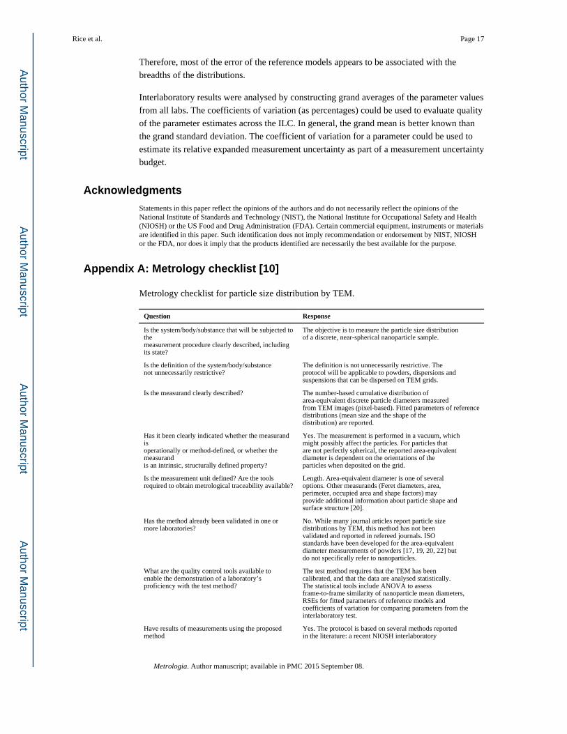
Metrology checklist for particle size distribution by TEM.

Question Response

Is the system/body/substance that will be subjected to themeasurement procedure clearly described, including its state?

The objective is to measure the particle size distributionof a discrete, near-spherical nanoparticle sample.

Is the definition of the system/body/substancenot unnecessarily restrictive?

The definition is not unnecessarily restrictive. Theprotocol will be applicable to powders, dispersions andsuspensions that can be dispersed on TEM grids.

Is the measurand clearly described? The number-based cumulative distribution ofarea-equivalent discrete particle diameters measuredfrom TEM images (pixel-based). Fitted parameters of referencedistributions (mean size and the shape of thedistribution) are reported.

Has it been clearly indicated whether the measurand isoperationally or method-defined, or whether the measurandis an intrinsic, structurally defined property?

Yes. The measurement is performed in a vacuum, whichmight possibly affect the particles. For particles thatare not perfectly spherical, the reported area-equivalentdiameter is dependent on the orientations of theparticles when deposited on the grid.

Is the measurement unit defined? Are the toolsrequired to obtain metrological traceability available?

Length. Area-equivalent diameter is one of severaloptions. Other measurands (Feret diameters, area,perimeter, occupied area and shape factors) mayprovide additional information about particle shape andsurface structure [20].

Has the method already been validated in one ormore laboratories?

No. While many journal articles report particle sizedistributions by TEM, this method has not beenvalidated and reported in refereed journals. ISOstandards have been developed for the area-equivalentdiameter measurements of powders [17, 19, 20, 22] butdo not specifically refer to nanoparticles.

What are the quality control tools available toenable the demonstration of a laboratory’sproficiency with the test method?

The test method requires that the TEM has beencalibrated, and that the data are analysed statistically.The statistical tools include ANOVA to assessframe-to-frame similarity of nanoparticle mean diameters,RSEs for fitted parameters of reference models andcoefficients of variation for comparing parameters from theinterlaboratory test.

Have results of measurements using the proposed method

Yes. The protocol is based on several methods reportedin the literature: a recent NIOSH interlaboratory

Rice et al. Page 17


Author M

anuscriptA

uthor Manuscript

Author M

anuscriptA

uthor Manuscript

Question Response

already been published in peer-reviewed journals byseveral laboratories?

comparison [13], a NIST protocol [14], and a genericprotocol from the National Physical Laboratory [15].

Is the required instrumentation widely available? Yes. TEM is widely available, but is costly to operate.Automated image capture and image analysis methods [32]are used to improve uniformity of measurements.

Does the document propose a measurementuncertainty budget?

Type A and B measurement uncertainties of the fittedparameters were assessed [30, 31, 33].

Appendix B: Definitions of statistical and metrological terms

Statistical definitions

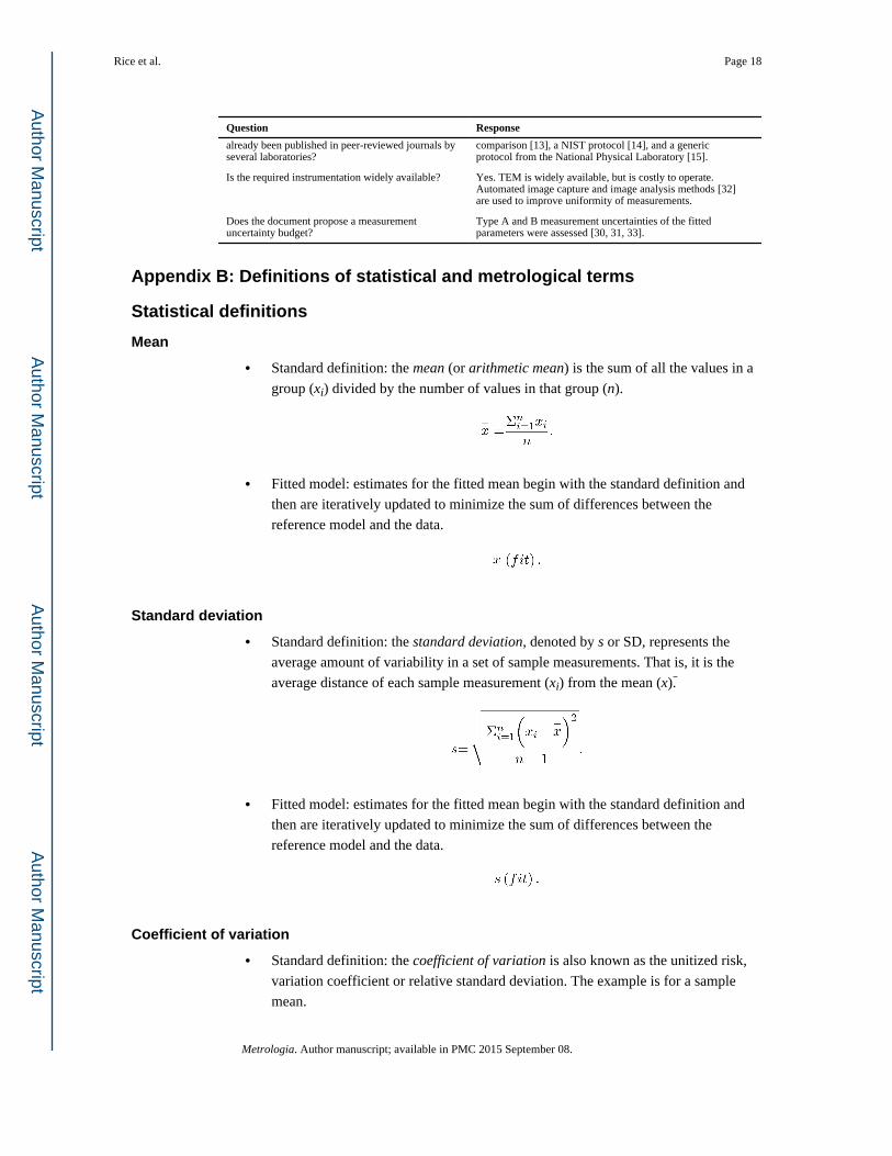
Mean

• Standard definition: the mean (or arithmetic mean) is the sum of all the values in a

group (xi) divided by the number of values in that group (n).

• Fitted model: estimates for the fitted mean begin with the standard definition and

then are iteratively updated to minimize the sum of differences between the

reference model and the data.

Standard deviation

• Standard definition: the standard deviation, denoted by s or SD, represents the

average amount of variability in a set of sample measurements. That is, it is the

average distance of each sample measurement (xi) from the mean (x).

• Fitted model: estimates for the fitted mean begin with the standard definition and

then are iteratively updated to minimize the sum of differences between the

reference model and the data.

Coefficient of variation

• Standard definition: the coefficient of variation is also known as the unitized risk,

variation coefficient or relative standard deviation. The example is for a sample

mean.

Rice et al. Page 18


Author M

anuscriptA

uthor Manuscript

Author M

anuscriptA

uthor Manuscript

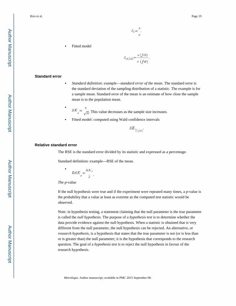
• Fitted model

Standard error

• Standard definition: example—standard error of the mean. The standard error is

the standard deviation of the sampling distribution of a statistic. The example is for

a sample mean. Standard error of the mean is an estimate of how close the sample

mean is to the population mean.

•. This value decreases as the sample size increases.

• Fitted model: computed using Wald confidence intervals

Relative standard error

The RSE is the standard error divided by its statistic and expressed as a percentage.

Standard definition: example—RSE of the mean.

•

.

The p-value

If the null hypothesis were true and if the experiment were repeated many times, a p-value is

the probability that a value at least as extreme as the computed test statistic would be

observed.

Note: in hypothesis testing, a statement claiming that the null parameter is the true parameter

is called the null hypothesis. The purpose of a hypothesis test is to determine whether the

data provide evidence against the null hypothesis. When a statistic is obtained that is very

different from the null parameter, the null hypothesis can be rejected. An alternative, or

research hypothesis, is a hypothesis that states that the true parameter is not (or is less than

or is greater than) the null parameter; it is the hypothesis that corresponds to the research

question. The goal of a hypothesis test is to reject the null hypothesis in favour of the

research hypothesis.

Rice et al. Page 19


Author M

anuscriptA

uthor Manuscript

Author M

anuscriptA

uthor Manuscript

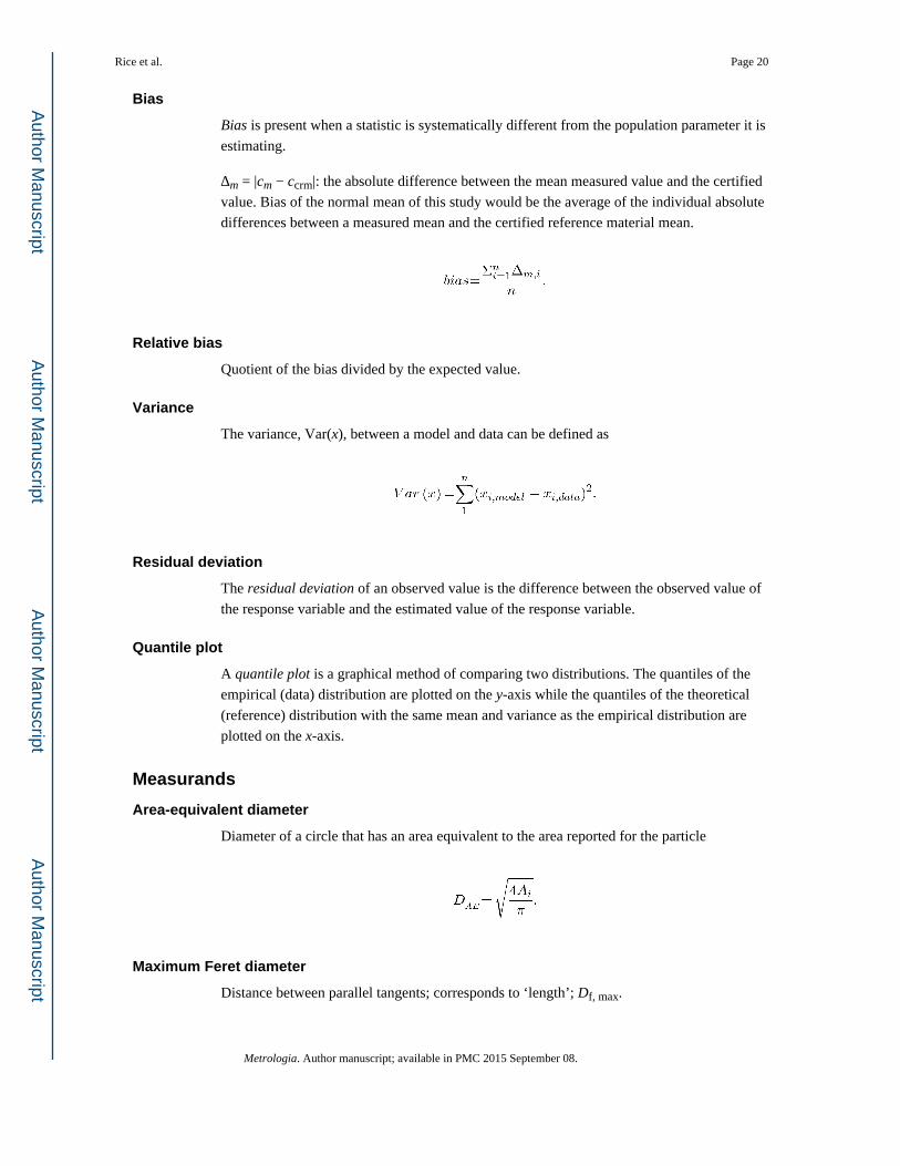
Bias

Bias is present when a statistic is systematically different from the population parameter it is

estimating.

Δm = |cm − ccrm|: the absolute difference between the mean measured value and the certified

value. Bias of the normal mean of this study would be the average of the individual absolute

differences between a measured mean and the certified reference material mean.

Relative bias

Quotient of the bias divided by the expected value.

Variance

The variance, Var(x), between a model and data can be defined as

Residual deviation

The residual deviation of an observed value is the difference between the observed value of

the response variable and the estimated value of the response variable.

Quantile plot

A quantile plot is a graphical method of comparing two distributions. The quantiles of the

empirical (data) distribution are plotted on the y-axis while the quantiles of the theoretical

(reference) distribution with the same mean and variance as the empirical distribution are

plotted on the x-axis.

Measurands

Area-equivalent diameter

Diameter of a circle that has an area equivalent to the area reported for the particle

Maximum Feret diameter

Distance between parallel tangents; corresponds to ‘length’; Df, max.

Rice et al. Page 20


Author M

anuscriptA

uthor Manuscript

Author M

anuscriptA

uthor Manuscript

Minimum Feret diameter

Distance between parallel tangents; corresponds to ‘breadth’; Df,min.

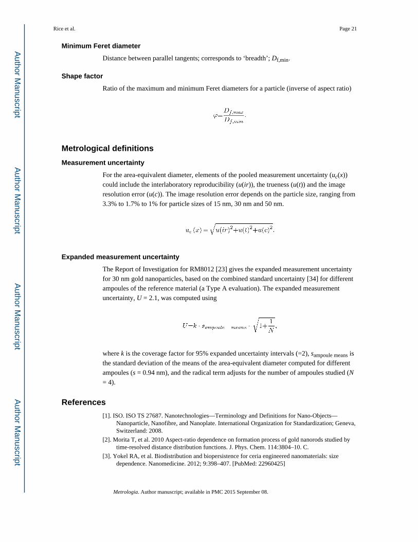
Shape factor

Ratio of the maximum and minimum Feret diameters for a particle (inverse of aspect ratio)

Metrological definitions

Measurement uncertainty

For the area-equivalent diameter, elements of the pooled measurement uncertainty (uc(x))

could include the interlaboratory reproducibility (u(ir)), the trueness (u(t)) and the image

resolution error (u(c)). The image resolution error depends on the particle size, ranging from

3.3% to 1.7% to 1% for particle sizes of 15 nm, 30 nm and 50 nm.

Expanded measurement uncertainty

The Report of Investigation for RM8012 [23] gives the expanded measurement uncertainty

for 30 nm gold nanoparticles, based on the combined standard uncertainty [34] for different

ampoules of the reference material (a Type A evaluation). The expanded measurement

uncertainty, U = 2.1, was computed using

where k is the coverage factor for 95% expanded uncertainty intervals (=2), sampoule means is

the standard deviation of the means of the area-equivalent diameter computed for different

ampoules (s = 0.94 nm), and the radical term adjusts for the number of ampoules studied (N

= 4).

References

[1]. ISO. ISO TS 27687. Nanotechnologies—Terminology and Definitions for Nano-Objects—Nanoparticle, Nanofibre, and Nanoplate. International Organization for Standardization; Geneva, Switzerland: 2008.

[2]. Morita T, et al. 2010 Aspect-ratio dependence on formation process of gold nanorods studied by time-resolved distance distribution functions. J. Phys. Chem. 114:3804–10. C.

[3]. Yokel RA, et al. Biodistribution and biopersistence for ceria engineered nanomaterials: size dependence. Nanomedicine. 2012; 9:398–407. [PubMed: 22960425]

Rice et al. Page 21


Author M

anuscriptA

uthor Manuscript

Author M

anuscriptA

uthor Manuscript

[4]. Macphail RC, Grulke EA, Yokel RA. Assessing nanoparticle risk poses prodigious challenges. Wiley Interdiscip. Rev. Nanomed. Nanobiotechnol. 2013; 5:374–87. [PubMed: 23568806]

[5]. EASAC-JRC. Impact of Engineering Nanomaterials on Health: Considerations for Benefit-Risk Assessment. E.A.S.A. Council. , editor. European Commission Joint Research Centre; Luxembourg: 2011. p. 9

[6]. Braun A, et al. Validation of dynamic light scattering and centrifugal liquid sedimentation methods for nanoparticle characterisation. Adv. Powder Technol. 2011; 22:766–70.

[7]. Couteau O, Roebben G. Measurement of the size of spherical nanoparticles by means of atomic force microscopy. Meas. Sci. Technol. 2011; 22:065101.

[8]. Linsinger, T., et al. Requirements on Measurements for the Implementation of the European Commission Definition of the Term ‘Nanomaterial’. E.C.J.R. Centre. , editor. Institute for Reference Materials and Measurements; Luxembourg: 2012.

[9]. Masuda H, Iinoya K. Theoretical study of the scatter of experimental data due to particle-size-distribution. J. Chem. Eng. Japan. 1970; 4:60–6.

[10]. ISO. Metrological check-list for the Preparation and Evaluation of ISO NWIPS and ISO WDs, ISO/TC 229N 673. 2008

[11]. Linsinger TPJ, et al. Reference materials for measuring the size of nanoparticles. TrAC, Trends Anal. Chem. 2011; 30:18–27.

[12]. ISO. ISO Guide 34. General Requirements for the Competence of Reference Material Producers. International Organization for Standardization (ISO); Geneva, Switzerland: 2009.

[13]. NIOSH. NIOSH/DUNE Interlaboratory Study: Evaluation of a Sample Preparation Technique for Determination of TEM-Based Size Distribution using NIST Reference Materials 8011, 8012, and 8013: gold nanoparticles. 2012:11. NIOSH/Dune Sciences.

[14]. Bonevich, JE.; Haller, WK. Measuring the size of nanoparticles using transmission electron microscopy (TEM). In: NIST. , editor. NIST-NCL Joint Assay Protocol, PCC-7 Version 1.1. NIST-NCL; Washington, DC: 2010. p. 13

[15]. Boyd RD, et al. Good practice guide for the determination of the size distribution of spherical nanoparticle samples. Measurement Good Practice Guide No 119. 2011 National Physical Laboratory.

[16]. ISO. ISO 9276-2 Representation of Results of Particle Size Analysis—Part 2: Calculation of Average Particle Sizes/Diameters and Moments From Particle Size Distributions. ISO; Geneva: 2001.

[17]. ISO. ISO 9276-3 Representation of Results of Particle Size Analysis—Part 3: Fitting of an Experimental Cumulative Curve to a Reference Model. ISO; Geneva: 2008.

[18]. ISO. ISO 9276-1 Representation of Results of Particle Size Analysis—Part 1: Graphical Representation. ISO; Geneva:

[19]. ISO. ISO 9276-5 Representation ofResults of Particle Size Analysis—Part 5: Methods of Calculation Relating to Particle Size Analyses using Logarithmic Normal Probability Distribution. ISO; Geneva: 2005. p. 12

[20]. ISO. ISO 9276-6 Representation of Results of Particle Size Analysis—Part 6: Descriptive and Quantitative Representation of Particle Shape and Morphology. ISO; Geneva: 2008. p. 23

[21]. ISO. Accuracy (Trueness and Precision) of Measurement Methods and Results—Part 1: General Principles and Definitions. ISO; Geneva: 5725. ISO

[22]. ISO. ISO 13322-1 Particle Size Analysis—Image Analysis Methods—Part 1: Static Image Analysis Methods. ISO; Geneva: 2004. p. 39

[23]. NIST. Report of Investigation. Reference Material 8012. Gold Nanoparticles, Nominal 30 nm Diameter. National Institute of Standards and Technology; Gaithersburg, MD: 2007. p. 10

[24]. Vladar, AE.; Ming, B. Measuring the size of colloidal gold nano-particles using high-resolution scanning electron microscopy. In: NIST. , editor. NIST-NCL Joint Assay Protocol, PCC-15. Version 1.1. NIST-NCL; Washington, DC: 2011. p. 20

[25]. Masuda H, Gotoh K. Study on the sample size required for the estimation of mean particle diameter. Adv. Powder Technol. 1999; 10:159–73.

Rice et al. Page 22


Author M

anuscriptA

uthor Manuscript

Author M

anuscriptA

uthor Manuscript

[26]. Song NW, et al. Uncertainty estimation of nanoparticle size distribution from a finite number of data obtained by microscopic analysis. Metrologia. 2009; 46:480–8.

[27]. Yoshida H, et al. Particle size measurement of standard reference particle candidates and theoretical estimation of uncertainty region. Adv. Powder Technol. 2009; 20:145–9.

[28]. Yoshida H, et al. Theoretical calculation of uncertainty region based on the general size distribution in the preparation of standard reference particles for particle size measurement. Adv. Powder Technol. 2012; 23:185–90.

[29]. JCGM. International Vocabulary on Metrology—Basic and General Concepts and Associated Terms (VIM). 2012 Available from: www.bipm.org/utils/common/documents/jcgm/JCGM_100_2008_E.pdf.

[30]. Kandil F. Measurement Uncertainty in Material Testing: Differences and Similarities between ISO, CEN, and ASTM approaches. 2011 Available from: www.vamas.org/documents/twa13/vamas_twa13_measurement_uncertainty_in_material_testing.pdf.

[31]. ISO. Guide to the Expression of Uncertainty in Measurement. International Organization for Standardization; Geneva, Switzerland: 1993.

[32]. Ferreira T, Rasband W. ImageJ User Guide IJ 1.45m. 2011 NIH.

[33]. Taylor, BN.; Kuyatt, CE. NIST Technical Note 1297. Washington, DC: 1994. Guidelines for evaluating and expressing the uncertainty of NIST measurement results.

[34]. NIST. Guidelines for evaluating and expressing the uncertainty of NIST measurement results. NIST Technical Note 1297. 1994 edBN Taylor andCE Kuyatt, National Institute of Standards and Technology.

Rice et al. Page 23


Author M

anuscriptA

uthor Manuscript

Author M

anuscriptA

uthor Manuscript

http://www.bipm.org/utils/common/documents/jcgm/JCGM_100_2008_E.pdf

http://www.bipm.org/utils/common/documents/jcgm/JCGM_100_2008_E.pdf

http://www.vamas.org/documents/twa13/vamas_twa13_measurement_uncertainty_in_material_testing.pdf

http://www.vamas.org/documents/twa13/vamas_twa13_measurement_uncertainty_in_material_testing.pdf

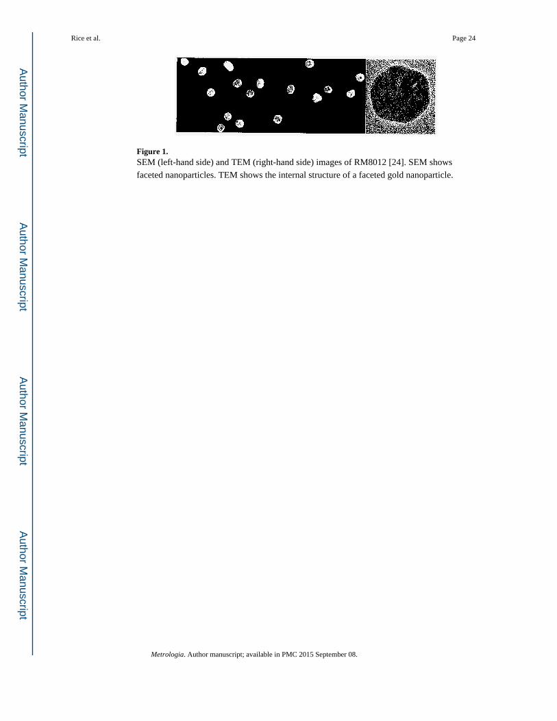
Figure 1. SEM (left-hand side) and TEM (right-hand side) images of RM8012 [24]. SEM shows

faceted nanoparticles. TEM shows the internal structure of a faceted gold nanoparticle.

Rice et al. Page 24


Author M

anuscriptA

uthor Manuscript

Author M

anuscriptA

uthor Manuscript

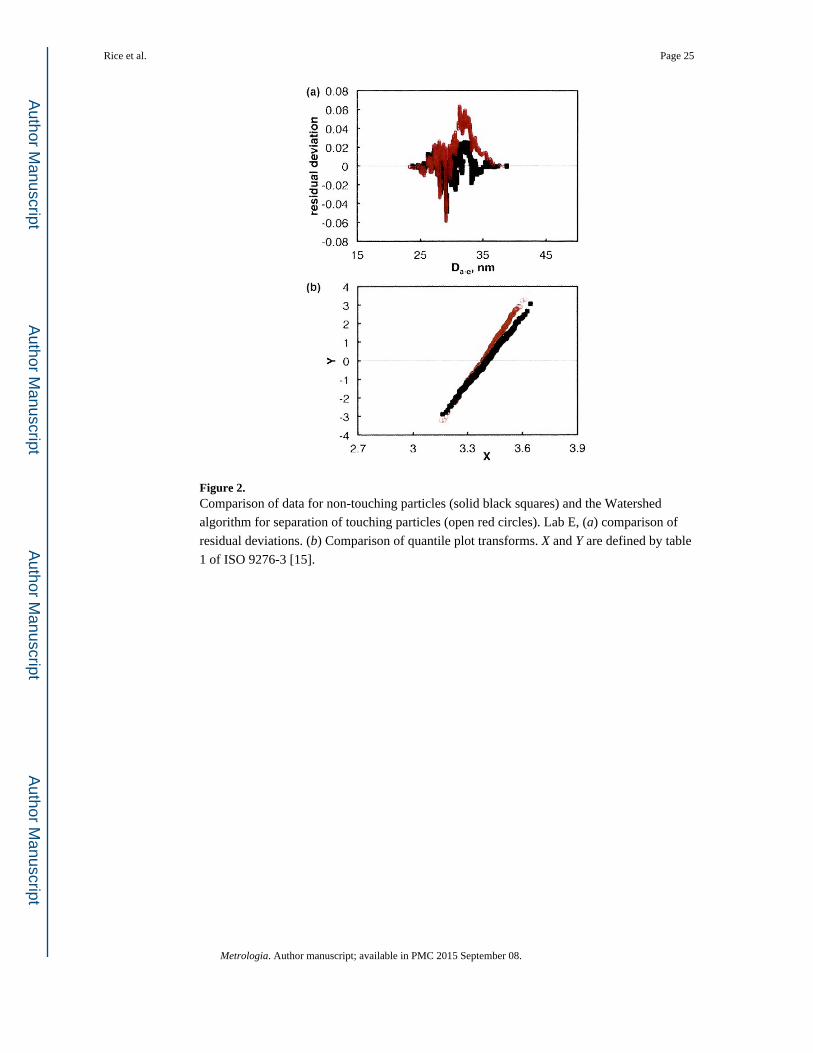
Figure 2. Comparison of data for non-touching particles (solid black squares) and the Watershed

algorithm for separation of touching particles (open red circles). Lab E, (a) comparison of

residual deviations. (b) Comparison of quantile plot transforms. X and Y are defined by table

1 of ISO 9276-3 [15].

Rice et al. Page 25


Author M

anuscriptA

uthor Manuscript

Author M

anuscriptA

uthor Manuscript

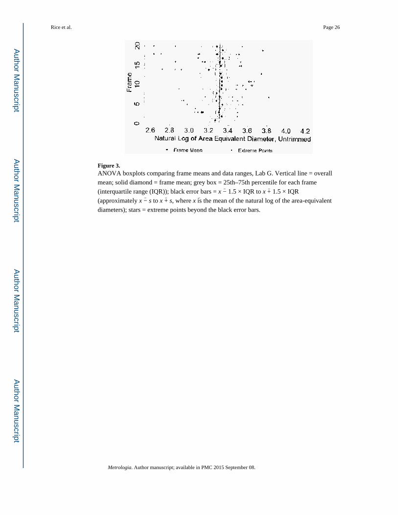
Figure 3. ANOVA boxplots comparing frame means and data ranges, Lab G. Vertical line = overall

mean; solid diamond = frame mean; grey box = 25th–75th percentile for each frame

(interquartile range (IQR)); black error bars = x − 1.5 × IQR to x + 1.5 × IQR

(approximately x − s to x + s, where x is the mean of the natural log of the area-equivalent

diameters); stars = extreme points beyond the black error bars.

Rice et al. Page 26


Author M

anuscriptA

uthor Manuscript

Author M

anuscriptA

uthor Manuscript

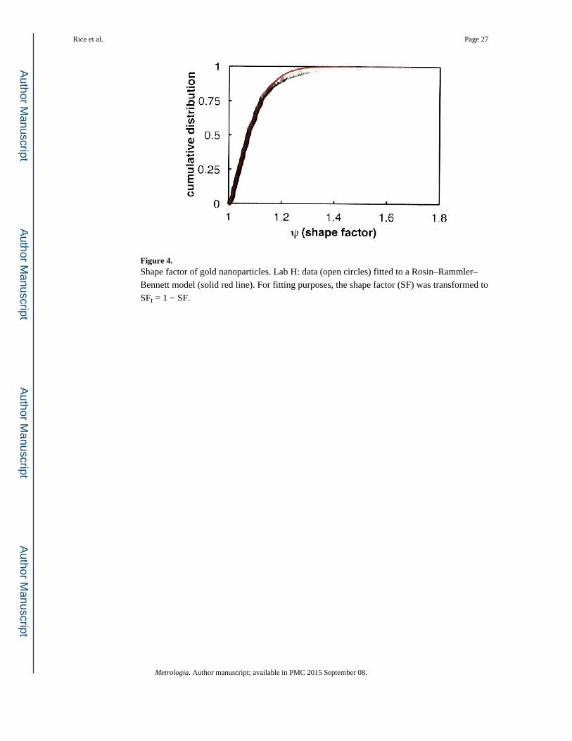
Figure 4. Shape factor of gold nanoparticles. Lab H: data (open circles) fitted to a Rosin–Rammler–

Bennett model (solid red line). For fitting purposes, the shape factor (SF) was transformed to

SFt = 1 − SF.

Rice et al. Page 27


Author M

anuscriptA

uthor Manuscript

Author M

anuscriptA

uthor Manuscript

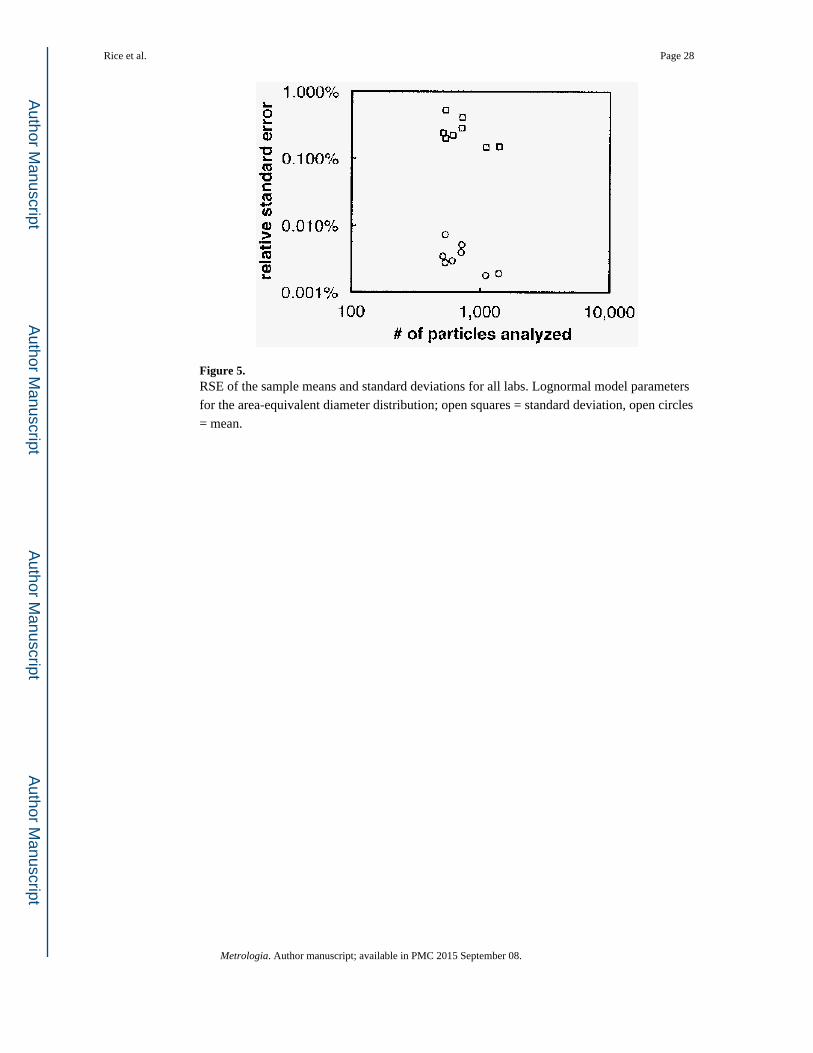
Figure 5. RSE of the sample means and standard deviations for all labs. Lognormal model parameters

for the area-equivalent diameter distribution; open squares = standard deviation, open circles

= mean.

Rice et al. Page 28


Author M

anuscriptA

uthor Manuscript

Author M

anuscriptA

uthor Manuscript

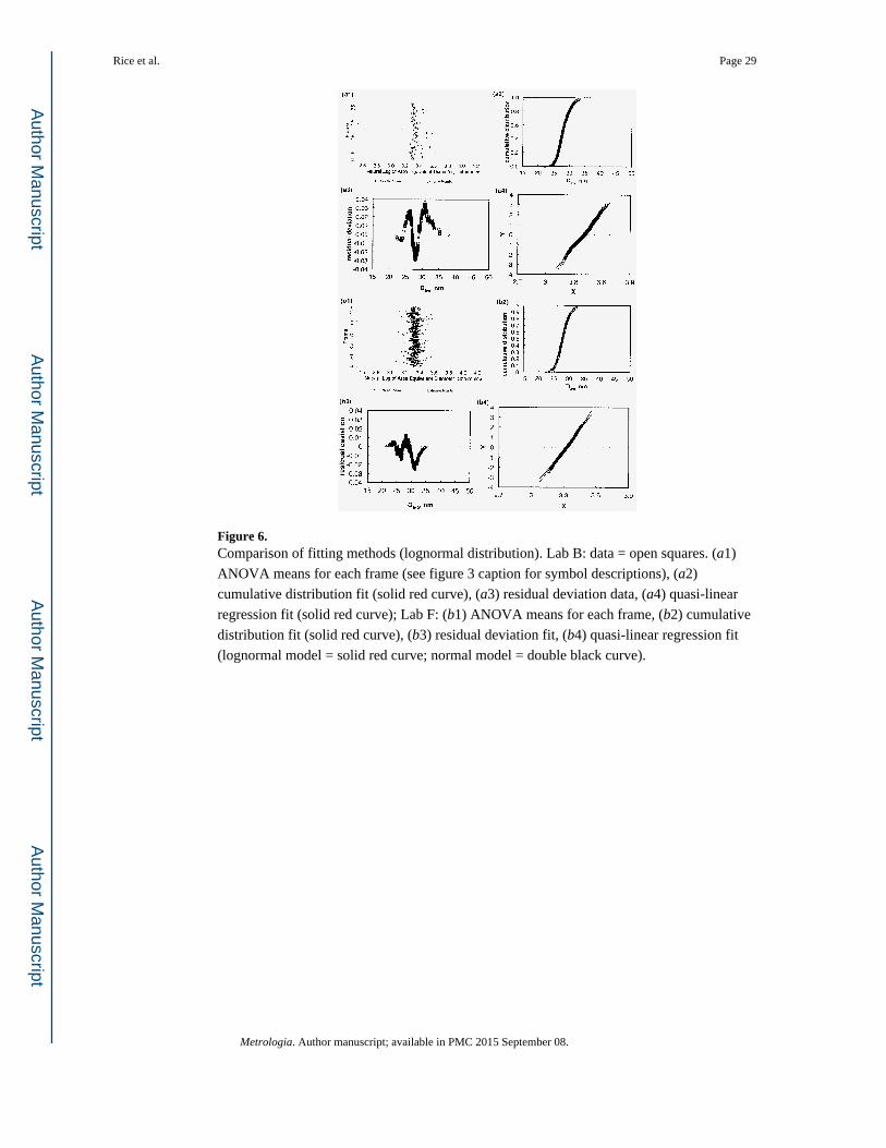
Figure 6. Comparison of fitting methods (lognormal distribution). Lab B: data = open squares. (a1)

ANOVA means for each frame (see figure 3 caption for symbol descriptions), (a2)

cumulative distribution fit (solid red curve), (a3) residual deviation data, (a4) quasi-linear

regression fit (solid red curve); Lab F: (b1) ANOVA means for each frame, (b2) cumulative

distribution fit (solid red curve), (b3) residual deviation fit, (b4) quasi-linear regression fit

(lognormal model = solid red curve; normal model = double black curve).

Rice et al. Page 29


Author M

anuscriptA

uthor Manuscript

Author M

anuscriptA

uthor Manuscript

Author M

anuscriptA

uthor Manuscript

Author M

anuscriptA

uthor Manuscript

Rice et al. Page 30

Table 1

Instrument factors.

Organization A B C D E F G H

# of frames analysed

62 49 20 27 11 135 20 55

# of nanoparticles analysed

706 624 535 513 608 1112 1480 531

Instrument JEOLJEM 2100

JEOL2000 FX

JeolJEM 1011

JEOL1011

JeolJEM 1220

FEITitan 80-300

FEI TecnaiG2 Twin

JEOL2010F

Acceleration voltage

200 kV 200 keV 80 kV 100 kV 80 kV 300 kV 200 kV 120 kV

Magnification 20 000× 21 000× nominal(~153 300×at camera)

100 000× 20 000× 40 000× 27 000× 19 000×,25000×,29 000×

20 000×

Frame size 1040 nm 1217.6 nm×811.2 nm

1320 nm×1700 nm

550 nm×550 nm

1000 nm×1400 nm

782 nm×782 nm

1875 nm×1875 nm

475 nm×475 nm

Pixel dimension 0.51nm/pixel

0.30nm/pixel

0.51nm/pixel

0.50nm/pixel

0.53nm/pixel

0.38nm/pixel

0.5nm/pixel

0.50nm/pixel

Image acquisition time per frame

3 s 4 s 5 s 4 s 3.5 s 0.5 s 3 s 3 s

Mean signal-to-noise ratio between background and particle

~2.5 ~14.2 2 ~2.4 2 ~2 2 ~2.5

Image analysis software

Image J Image J Image J Image J Image J Image J Image J Image J


Author M

anuscriptA

uthor Manuscript

Author M

anuscriptA

uthor Manuscript

Rice et al. Page 31

Table 2

ANOVA for the natural logarithm of three measurands: (A) area-equivalent diameter, (B) maximum Feret

diameter and (C) shape factor. The p-values rejecting the null hypothesis of all frames having equal means are

italicized (p < 0.05).

(A) Natural log of area equivalent

Area-equivalentdiameter/nm

Laboratoryx‒

∕ ln(nm)s/ln(nm) p-value

A 3.34 0.0066 0.711 28.6

B 3.33 0.0030 0.0001 27.9

C 3.33 0.0036 0.274 27.9

D 3.27 0.0067 0.168 26.4

E 3.28 0.0031 0.0010 26.7

F 3.33 0.0023 0.0026 28.0

G 3.31 0.0026 <0.0001 27.5

H 3.31 0.0038 0.106 27.4

(B) Natural log of Feret diameter

Feretdiameter/nm

Laboratoryx‒

∕ ln(nm)s/ln(nm) p-value

A 3.43 0.0069 0.758 31.2

B 3.40 0.0035 0.0005 30.1

C 3.41 0.0043 0.342 30.5

D 3.36 0.0065 0.413 29.0

E 3.40 0.0033 <0.0001 30.2

F 3.43 0.0030 0.138 30.9

G 3.42 0.0027 <0.0001 30.6

H 3.39 0.0040 0.0054 29.8

(C) Natural log of aspect ratio

Mean aspectratio

Laboratoryx‒ s p-value

A 0.100 0.0036 0.904 1.11

B 0.098 0.0034 0.351 1.11

C 0.123 0.0065 <0.0001 1.15

D 0.107 0.0042 0.290 1.12

E 0.107 0.0041 0.0003 1.12

F 0.109 0.0035 0.961 1.12

G 0.108 0.0027 0.0051 1.12

H 0.089 0.0032 0.0459 1.10


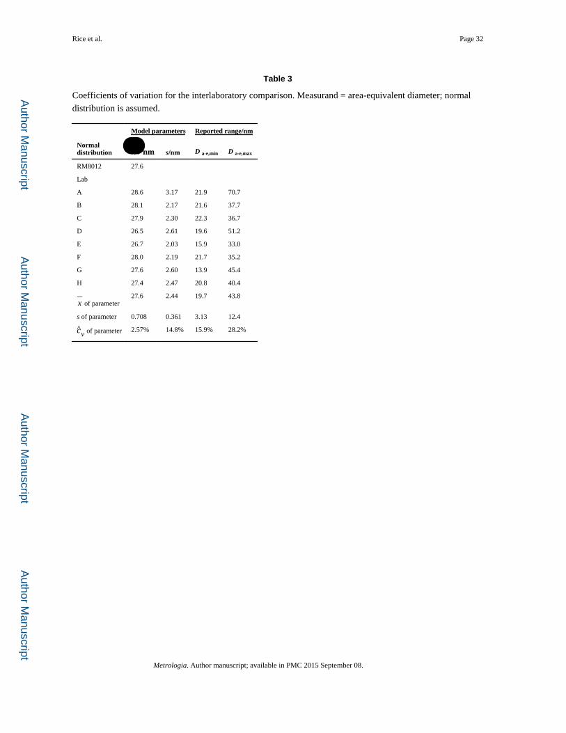
Author M

anuscriptA

uthor Manuscript

Author M

anuscriptA

uthor Manuscript

Rice et al. Page 32

Table 3

Coefficients of variation for the interlaboratory comparison. Measurand = area-equivalent diameter; normal

distribution is assumed.

Normaldistribution

Model parameters Reported range/nm

x‒

∕ nm s/nm D a-e,min D a-e,max

RM8012 27.6

Lab

A 28.6 3.17 21.9 70.7

B 28.1 2.17 21.6 37.7

C 27.9 2.30 22.3 36.7

D 26.5 2.61 19.6 51.2

E 26.7 2.03 15.9 33.0

F 28.0 2.19 21.7 35.2

G 27.6 2.60 13.9 45.4

H 27.4 2.47 20.8 40.4

x‒

of parameter27.6 2.44 19.7 43.8

s of parameter 0.708 0.361 3.13 12.4

cv of parameter 2.57% 14.8% 15.9% 28.2%


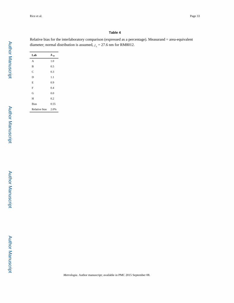
Author M

anuscriptA

uthor Manuscript

Author M

anuscriptA

uthor Manuscript

Rice et al. Page 33

Table 4

Relative bias for the interlaboratory comparison (expressed as a percentage). Measurand = area-equivalent

diameter; normal distribution is assumed, = 27.6 nm for RM8012.

Lab Δ m

A 1.0

B 0.5

C 0.3

D 1.1

E 0.9

F 0.4

G 0.0

H 0.2

Bias 0.55

Relative bias 2.0%


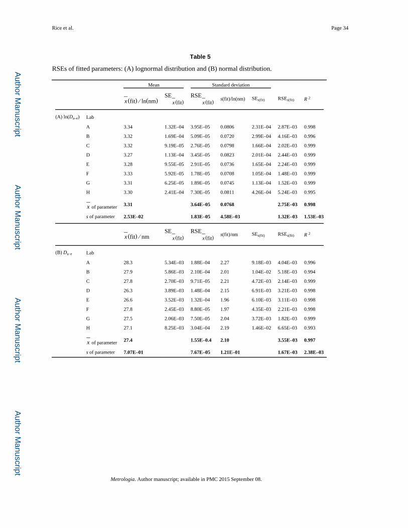
Author M

anuscriptA

uthor Manuscript

Author M

anuscriptA

uthor Manuscript

Rice et al. Page 34

Table 5

RSEs of fitted parameters: (A) lognormal distribution and (B) normal distribution.

Mean Standard deviation

x‒

(fit) ∕ ln(nm)SE

x‒

(fit)RSE

x‒

(fit)s(fit)/ln(nm) SEs(fit) RSEs(fit) R 2

(A) ln(Da–e) Lab

A 3.34 1.32E–04 3.95E–05 0.0806 2.31E–04 2.87E–03 0.998

B 3.32 1.69E–04 5.09E–05 0.0720 2.99E–04 4.16E–03 0.996

C 3.32 9.19E–05 2.76E–05 0.0798 1.66E–04 2.02E–03 0.999

D 3.27 1.13E–04 3.45E–05 0.0823 2.01E–04 2.44E–03 0.999

E 3.28 9.55E–05 2.91E–05 0.0736 1.65E–04 2.24E–03 0.999

F 3.33 5.92E–05 1.78E–05 0.0708 1.05E–04 1.48E–03 0.999

G 3.31 6.25E–05 1.89E–05 0.0745 1.13E–04 1.52E–03 0.999

H 3.30 2.41E–04 7.30E–05 0.0811 4.26E–04 5.24E–03 0.995

x‒

of parameter 3.31 3.64E–05 0.0768 2.75E–03 0.998

s of parameter 2.53E–02 1.83E–05 4.58E–03 1.32E–03 1.53E–03

x‒

(fit) ∕ nmSE

x‒

(fit)RSE

x‒

(fit)s(fit)/nm SEs(fit) RSEs(fit) R 2

(B) Da–e Lab

A 28.3 5.34E–03 1.88E–04 2.27 9.18E–03 4.04E–03 0.996

B 27.9 5.86E–03 2.10E–04 2.01 1.04E–02 5.18E–03 0.994

C 27.8 2.70E–03 9.71E–05 2.21 4.72E–03 2.14E–03 0.999

D 26.3 3.89E–03 1.48E–04 2.15 6.91E–03 3.21E–03 0.998

E 26.6 3.52E–03 1.32E–04 1.96 6.10E–03 3.11E–03 0.998

F 27.8 2.45E–03 8.80E–05 1.97 4.35E–03 2.21E–03 0.998

G 27.5 2.06E–03 7.50E–05 2.04 3.72E–03 1.82E–03 0.999

H 27.1 8.25E–03 3.04E–04 2.19 1.46E–02 6.65E–03 0.993

x‒

of parameter 27.4 1.55E–0.4 2.10 3.55E–03 0.997

s of parameter 7.07E–01 7.67E–05 1.21E–01 1.67E–03 2.38E–03


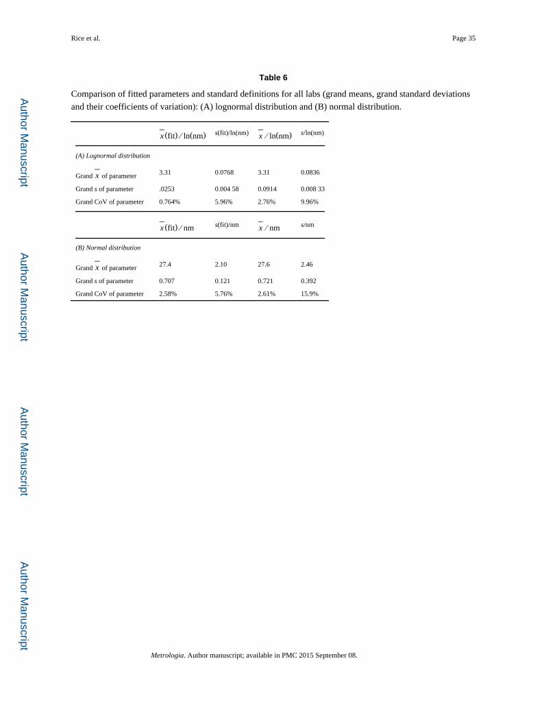
Author M

anuscriptA

uthor Manuscript

Author M

anuscriptA

uthor Manuscript

Rice et al. Page 35

Table 6

Comparison of fitted parameters and standard definitions for all labs (grand means, grand standard deviations

and their coefficients of variation): (A) lognormal distribution and (B) normal distribution.

x‒

(fit) ∕ ln(nm) s(fit)/ln(nm) x‒

∕ ln(nm) s/ln(nm)

(A) Lognormal distribution

Grand x‒

of parameter 3.31 0.0768 3.31 0.0836

Grand s of parameter .0253 0.004 58 0.0914 0.008 33

Grand CoV of parameter 0.764% 5.96% 2.76% 9.96%

x‒

(fit) ∕ nm s(fit)/nm x‒

∕ nm s/nm

(B) Normal distribution

Grand x‒

of parameter 27.4 2.10 27.6 2.46

Grand s of parameter 0.707 0.121 0.721 0.392

Grand CoV of parameter 2.58% 5.76% 2.61% 15.9%


Documents

HHS Public Access 1 Scott C Brown Peter Eschbach Li Han