1

Heterogeneous Preferences and the Efficacy of Public School Choice

by

Justine S. Hastings Department of Economics Yale University and NBER

Thomas J. Kane

Harvard Graduate School of Education and NBER

Douglas O. Staiger

Department of Economics Dartmouth College and NBER

ABSTRACT

Public school choice plans are intended to increase equity and quality in education by offering students at under-performing schools immediate academic gains from attending a higher-achieving school and by creating demand-side pressure on under-performing schools to improve. We develop a model to show how these gains from choice depend on heterogeneity in how parents choose schools, and test the model’s predictions using data on parental choices and lottery assignments to schools from a school choice plan in Charlotte, North Carolina. We estimate an exploded-mixed-logit model of demand for schools and find that higher-SES parents are more likely to choose higher-performing schools, while minority families must trade off preferences for high-performing schools against preferences for a predominantly minority school. These differences in choice behavior lead to low demand-side pressure for improvement at schools serving low-SES and minority families relative to those serving high-SES families. In addition, we find that children of parents placing high weight on academic achievement experience test score gains from moving to their preferred schools, while others experience no gain or declines in test scores. This is particularly true for minority families who must sacrifice attending a predominantly minority school to select a high-test-score school. Our results imply that public school choice may widen rather than narrow the gap in achievement. ______________________________________ This paper was previously circulated as Hastings, Kane, and Staiger (2007a) and (2007b). This paper combines and replaces those two papers. We thank the Charlotte-Mecklenburg School Board, Office of the Superintendent, as well as the excellent school district staff for making this project possible. We thank the editor, three anonymous referees, Joseph Altonji, Patrick Bayer, Steven Berry, David Card, Philip Haile, Carolyn Hoxby, Fabian Lange, Derek Neal, Sharon Oster, Miguel Villas-Boas, Sofia Villas-Boas, and numerous seminar participants for helpful comments and suggestions at various stages of the project. C. Sean Hundtofte and Jeffrey Weinstein provided outstanding research assistance. The project is funded by grants from the Institution for Social and Policy Studies at Yale University and the U.S. Department of Education.

2

1. Introduction

Several urban public school districts are currently experimenting with public school

choice plans, and the federal No Child Left Behind Act of 2001 includes a choice provision

allowing parents of children in failing schools to send their children to non-failing schools

outside of their neighborhood. The goal of these school-choice plans is two-fold. First, school

choice allows disadvantaged students the immediate opportunity to benefit academically from

attending a higher-performing school. Second, school choice is intended to increase pressure on

failing schools to improve through the threat of losing students, thereby improving educational

equity.

Both of these potential benefits from public school choice implicitly assume that all

parents value academics highly and will choose schools accordingly once residential restrictions

are lifted. However, parents may have a variety of reasons for choosing schools, and differences

in preferences and school choices may generate both heterogeneous short-run effects of attending

a first choice school on academic outcomes (Heckman (1997), Heckman, Smith, and Clements

(1997), Heckman, Urzua, and Vytlacil (2006)) and disparate demand-side pressure for academic

improvement across low-achieving and high-achieving schools (e.g., vertical differentiation in a

differentiated products market, Anderson, de Palma, and Thisse (1992)). For example, if

disadvantaged families place less weight on academics when choosing schools, then schools

serving these families will face little pressure to improve, and children of these families may not

reap academic gains from changing schools. If this is the case, then school choice may have the

smallest immediate impact on the families it is intended to help, and cause greater educational

stratification over time. While the prior literature has postulated the range of potential impacts

school choice could have on the achievement gap (Hanushek (1981), Hoxby (2002, 2003)), there

is very little empirical evidence identifying heterogeneity in parental choices and the link

between choice behavior and academic outcomes.

In this paper, we use a unique dataset and policy experiment from the Charlotte-

Mecklenburg School Public School District (CMS) in North Carolina to examine heterogeneity

in parental school choice behavior and its implications for public school choice. We use data on

parents’ multiple-ranked choices for schools during the implementation of district-wide school

choice in 2002 to estimate an exploded-mixed-logit demand model for schools, allowing

3

heterogeneity to influence choice behavior through both observable and unobservable family

characteristics. We find that the weights parents place on key school characteristics are very

heterogeneous, with high-income parents of high-achieving students placing the largest weights

on test scores when selecting schools. In addition, we show that parents of each race prefer

schools where their own race is the clear majority, implying that minority parents face much

larger tradeoffs between academics and social preferences when choosing schools.

We then use our demand estimates to examine the ability of school choice to increase

pressure on low-performing schools to improve through the threat of losing students. To do this,

we simulate the demand response that would result if a school were to boost average test scores,

holding all else constant. We find that demand-side pressure is largest for high-performing

schools that serve very elastic families and minimal for low-performing schools that serve

inelastic, disadvantaged families. These results suggest that public school choice, without

additional incentive mechanisms, may lead to greater educational stratification of schools serving

high- and low-income families, rather than providing a competitive tide that lifts all boats.

Finally, we examine how heterogeneity in choice behavior affects the immediate gains in

test scores from attending a first choice school for children from advantaged versus

disadvantaged backgrounds. CMS used lotteries to assign students to oversubscribed schools,

allowing us to identify the causal effect of attending a first choice school on gains in own

academic achievement. Theory suggests that the academic gains from attending a first choice

school will be positive for parents who place a high weight on academics but potentially negative

for parents who place a low weight on academics and high weights on other school

characteristics that are negatively correlated with academics. Using the exploded-mixed-logit

model to estimate the weight that each parent placed on test scores when choosing a school, we

find that students of parents with weights at the 95th percentile experienced significant rises in

End of Grade test scores of approximately 0.1 student-level standard deviations, while students

of parents placing little value on academics actually experienced declines in achievement. These

declines were strongest for African American families that placed little weight on academics,

since they generally prefer schools with more minority students (which in CMS tend to be

schools with lower academic performance). These results imply that the immediate impact of

attending a first choice school broadens (instead of narrows) the gap in performance across high-

and low-SES families exercising choice, and highlight how the school choice tradeoffs minority

4

parents face between academic achievement and social match may reinforce the achievement

gap.

This paper makes a number of contributions. First, it examines the potential efficacy of

public school choice by estimating the underlying determinants of parents’ choices. We are able

to identify heterogeneity in choice parameters in our model because we have rich micro data

with multiple-ranked choices (Berry, Levinsohn, and Pakes (2004)), variation in choice set

characteristics from large-scale redistricting with the introduction of the school choice plan, and

a diverse underlying student-body population. While prior papers have examined aspects of

parental choice using a variety of measures from survey responses to residential location

decisions (Armor and Peiser (1998), Vanourek et al. (1998), Greene et al. (1997), Kleitz et al.

(2000), Schneider et al. (1998), Glazerman (1997), Nechyba (1999, 2000, 2003), Epple and

Romano (1998, 2002), Bayer, Ferreira and McMillan (2004)), they have not estimated

heterogeneity in parental choices nor linked this with demand-side pressure to improve

academics and gains from attending a first choice school.

Second, our approach allows us to examine if school choice will provide stronger

demand-side pressure for low-performing schools to improve or if it will result in greater

stratification across schools serving low- and high-SES families. The prior literature has focused

on estimating competitive pressure and its impact on academic achievement, using aggregated

data and measures such as HHIs (Herfindahl-Hirschman Indices) of local districts as proxies for

competition (Borland and Howsen (1992), Hoxby (2000), Hanushek and Rivkin (2003), Belfield

and Levin (2002)). This implicitly assumes that all schools (or districts) face homogeneous

demand elasticity and competitive pressure with respect to average test scores (Farrell and

Shapiro (1990)). Expanding on this literature, Rothstein (2006) investigated the possibility that

parents may choose schools based on factors other than academic achievement, but maintained a

similar HHI framework and aggregated analysis for measuring competition. Modeling consumer

(parental) choice for differentiated products (schools) allows different types of schools to face

different demand elasticities, and thus we can test how public school choice may affect demand-

side incentives to improve quality across low- and high-achieving schools.

Finally, we provide an economic explanation for why certain subgroups of students

benefit from exercising choice. Several recent papers have estimated the average treatment effect

of winning a lottery to attend a first choice school, abstracting away from the underlying factors

5

that led parents to select these schools. Cullen, Jacob, and Levitt (2006) examine high school

lotteries in Chicago and find no significant average impact on test scores from attending a chosen

school, leading them to conclude that measurable school inputs have little causal impact on

student outcomes. Others studies find positive outcomes for some subgroups or for students

applying to different types of schools, but the results vary across studies (Ballou (2007), Betts et

al. (2006), Hastings, Kane and Staiger (2006)). By connecting expected treatment effects with

choice behavior and the tradeoffs parents face when choosing schools, we provide a framework

for understanding why subgroup impacts may vary across studies and across student groups as

preferences, tradeoffs, and choice sets vary.

This paper proceeds in four sections. The next section provides background on the CMS

school choice plan. Section 3 presents our empirical model and outlines testable implications for

the efficacy of public school choice. Section 4 presents our empirical results, including a

description of the data, estimates from the exploded-mixed-logit model, demand simulations, and

estimates of the gains from attending a first choice school. The final section concludes with some

thoughts on the implications these results have for the design of school choice.

2. The CMS School Choice Plan

Before the introduction of a school choice plan in the fall of 2002, the Charlotte-

Mecklenburg Public School District (CMS) operated under a racial desegregation order for three

decades. In September 2001, the U.S. Fourth Circuit Court of Appeals declared the school

district “unitary” and ordered it to dismantle the race-based student assignment plan by the

beginning of the next school year. In December of 2001, the school board voted to approve a

new district-wide public school choice plan.

In the spring of 2002, parents were asked to submit their top three choices of school

programs for each of their children. Each student was assigned a “home-school” in her

neighborhood, often the closest school to her, and was guaranteed a seat at this school. Magnet

students were similarly guaranteed admission to continue in their current magnet programs.

Admission for all other students was limited by grade-specific capacity limits set by the district.

Parents could choose any school in the district. However, transportation was only provided to

schools in a student’s quadrant of the district (the district was split into four quadrants called

6

“Choice Zones”). The district allowed significant increases in enrollment in many schools in the

first year of the school choice program in an expressed effort to give each parent one of her top

three choices. In the spring of 2002, the district received choice applications from approximately

105,000 of 110,000 students. Admission to oversubscribed schools was determined by a lottery

system as described below.

Once the district was declared “unitary” and the court order requiring race-based busing

was terminated, CMS could no longer draw boundaries based on the racial composition of a

neighborhood. As a result, the former school assignment zones, which often paired non-

contiguous black and white neighborhoods, were dramatically redrawn. Under the choice plan,

43 percent of parcels were assigned to a different elementary grade “home-school” than they

were assigned to the year before under the busing system. At the middle school and high school

levels, this number was 52 and 35 percent, respectively. Therefore, the 2002-2003 home-school

for many students was often not the school they would have been assigned at the time they chose

their residence. This dramatic change in school assignment zones, the simultaneous introduction

of a sweeping school choice plan, and the assignment of students to high demand schools by

lottery provides a unique opportunity to examine the implications of parental choice behavior for

achievement of disadvantaged students in a public school choice plan.

2.1 Heterogeneous Choices

Table I provides an overview of student characteristics and parents’ choices in our

sample, broken down by race and lunch subsidy status.Throughout the analysis, we focus on

students entering grades four through eight because of the lack of test scores for other grades

(details on the data and estimation sample are provided in Section 4). Whites and Blacks each

comprised approximately 45 percent of the student-body population. Approximately 10 percent

of white students received federal lunch subsidies, while just over 60 percent of African

Americans did. Minority and lunch-subsidy recipients had, on average, lower achievement (test

scores were from Spring 2002 and standardized to have a mean of zero and a standard deviation

of one across all students within each grade) and came from lower income neighborhoods, but

there was substantial variation in test scores and income within group as well. Neighborhood

income is measured as the median income for families living in a student’s census block group of

the student’s same race according to the 2000 Census.

7

In addition, minority and lunch-subsidy students had lower-performing home-schools as

measured by average student test scores.1 However, because CMS had previously bused students

of all races to schools in different neighborhoods, as well as to “midpoint” schools between

neighborhoods, most students faced a diverse set of school choices within reasonable distance

from their homes. On average, elementary school students had sixteen school choice options

within a 12 mile driving radius from their home, and middle school students had six. On average

the home-school was about three miles away from the student's house (a bit further for white

non-lunch recipient students who are more likely to reside in outer suburbs). However, the next

closest non-home-school option was on average only a slightly further drive. Table I shows that

students had a considerable range of school test scores at school choice options within six miles

(approximately twice the distance to the home-school). Across the district, school test scores

range from approximately negative one to one, so students of all socioeconomic backgrounds

had schools ranging from the lower to the upper quartile within reasonable proximity. Although

test scores at the top scoring school within six miles are on average higher for non-poor white

families, the standard deviation is large, and the variation in school average test scores for

proximate schools is substantial for all socioeconomic groups. This variation along with multiple

choices will help identify the underlying determinants of parents’ school choices.2

Since parents were guaranteed a slot in their default school, many parents listed only one

or two schools on their choice forms. Table I indicates that parents of students who were white

and ineligible for lunch subsidies were approximately twice as likely as non-white-lunch-

recipient student to choose their home-school as their first choice, which is consistent with the

difference in average home-school test score across the two groups. Overall, parents of white,

lunch-ineligible students were also much more likely to list only one choice than parents in the

other subgroups. Parents of free-lunch eligible non-white children were most likely to list three

choices. Many parents listed subsequent choices after listing their home-school option, despite

the fact that admission to the home-school was guaranteed. Of parents who chose the home-

school first or second, 27.4, 43.0, 39.2 and 50.9 percent, across the four race and income

categories respectively, listed subsequent choices beyond the guaranteed option. Listing

additional choices took little time (particularly if parents had already considered alternative

1 School average test scores were calculated as the average of the combined standardized 2001-2002 test score for students attending the school in the 2002-2003 school year. See Section 4 for details. 2 For maps of school options and student characteristics in CMS see Hastings, Kane and Staiger (2007a).

8

schools in making their choice), and doing so when the form allowed it was a reasonable

precaution when parents lacked complete understanding of or confidence in the process.3

Despite the proximity of high-performing schools to neighborhoods of various

socioeconomic backgrounds, there was little unanimity in parents’ choices of schools. Even

within the same elementary home-school assignment for 2002-2003, parents listed, on average,

10.4 different first choice elementary schools.

The

availability of multiple choices from those parents who listed their home-school first or second

adds further choice set variation and aids in the identification of demand parameters, although

estimates were similar between such parents and the sample as a whole.

4 It is clear that parents have very heterogeneous

preferences over school characteristics. Figure 1 shows that approximately 20 percent of parents

chose schools that had lower test scores than the school they had guaranteed admission to,

suggesting that school characteristics that were potentially negatively correlated with average

test scores were the strongest determinants of choice for some families. This suggests that

heterogeneous preferences may play a key role in school selection and academic outcomes in

public school choice.5

3 Non-white and free-lunch parents may also have been less likely to use the automated phone system to choose, which ceased prompting for additional choices after the home -school was chosen. 4 This number accounts for differences in choices listed driven by differences in the prior-year’s school. 5 Hastings and Weinstein (2008) find less heterogeneity, with most parents choosing schools with higher test scores, when they receive simplified information on school test scores. Our model of parental choice in Section 3 allows heterogeneity in preferences to be interpreted as heterogeneity in information costs in collecting and/or interpreting measures school academic quality.

2.2 Lottery Assignments

The district implemented a lottery system for determining admissions to oversubscribed

schools. Approximately one third of the schools in the district were oversubscribed. Under the

lottery system, students choosing non-home-schools were first assigned to priority groups, and

student admission was then determined by a lottery number. The priority groups for district

schools were arranged in lexicographic order based on the following priorities:

Priority 1: Student who had attended the school in the prior year (students were subdivided

into three priority groups depending upon their grade level, with students in terminal

grades—grades five, eight, and 12—given highest priority).

9

Priority 2: Parent of free-lunch eligible student applying to school where less than half the

students were free-lunch eligible

Priority 3: Parent applying to a school within her choice zone

Parents listing a given school as their first choice were sorted by priority group and a

randomly assigned lottery number.6 Any slots remaining after home-school students were

accommodated were assigned in order of priority group and random number.7

The lottery mechanism used by CMS was a “first-choice-maximizer”, in which slots were

first assigned to all those listing a given school as a first choice before moving to those listing the

school as a second or third choice. In such a mechanism, parents with poor home-school options

may have an incentive to misstate their preferences – not listing their most preferred school if it

had a low probability of admission (Glazerman and Meyer (1995), Abdulkadiroğlu and Sönmez

(2003), Abdulkadiroğlu et al. (2006)). Instead, they may have hedged their bets by listing a less

If a school was not

filled by those who had listed it as a first choice, the lottery would repeat the process with those

listing the school as a second choice, using the same priority groups as above. However, for

many oversubscribed schools, the available spaces were filled up by the time the second choice

priority groups came up.

Children of parents not assigned to one of their top choices were placed on a waiting list.

About 19 percent of students winning the lottery to attend their parents’ first choice schools

subsequently attended a different school, with 13 percent attending their home-schools instead

and another six percent attending a different school entirely, with most of these students

changing address. When slots became available, students were taken off the waitlist based on

their lottery numbers alone, without regard for their priority groups.

2.3 Potential for Strategic Choice

6 The random number was assigned by a computer using an algorithm that we verified with CMS computer programmers. We also verified the randomization using the lottery and student assignment data. 7 The choice program allowed for sibling admissions in the following way. If a parent had two children in the same grade level (i.e. both in middle school), and listed the same school as the first choice for both children, then once one child was admitted the second child was also admitted. No preference was given to siblings in different grade levels, e.g. a child choosing an elementary school that feeds into a sibling’s first choice middle school. When we turn to estimate the effects of attending a first choice school on academic outcomes, we will only use students for whom lottery number alone determined admission, which will consequently exclude the few students who were admitted to their first choice school based on a sibling’s lottery number.

10

preferred option with a higher probability of admission in order to avoid being assigned to their

home-school. Such strategic behavior would imply that parental choices would not reflect true

preference orderings for schools – to the extent that parents are not listing their preferred match

due to strategic hedging.

However, there were a number of reasons why such strategic behavior was probably rare

in the first year of the choice plan that we are studying. First, this was a new school choice plan,

and parents did not know the details of how the lottery system would be operated. The handful of

district officials who knew the lottery details were not allowed to communicate them to parents,

and parents were never given their actual lottery numbers.8 The district also told parents that they

would make every attempt to give each student admission to one of their chosen schools and

instructed them to list what they wanted.9

If there were widespread strategic behavior by parents, we would expect those with low-

quality default schools to hedge their bets and list less desirable schools for which they might

have a higher probability of admission. Hastings, Kane and Staiger (2007a) use the redistricting

to test if parents with exogenous changes to the quality of their home-school had lower

preferences for high-quality schools, as would be predicted if parents were behaving

strategically, and they find no evidence that this was the case. We discuss this evidence in more

Even in long-standing limited choice plans where

districts instruct parents to choose strategically, there is evidence that many parents do not act

strategically (Pathak and Sönmez (2008)). To accommodate demand, the district substantially

expanded capacity at popular schools. In addition, the district gave a “priority boost” to low-

income students choosing to attend schools with low concentrations of low-income students.

Hence, choices for top schools by students with underperforming home-schools would be given

top priority. This would counteract the incentive for these students to hedge their choices, as

outlined above.

8 Parents were given a choice booklet to aid with their school choice decision, which stated that "Students will be chosen through a lottery process in the following order of priority:" and then listed the priorities outlined above. This was the only description of the lottery given. 9 Specifically, the school choice booklet instructed parents to read the school descriptions, decide what their first, second and third choices were, and complete the choice application worksheet. It also stated that every student must apply or they would not be guaranteed a seat at their home-school. They were given a help line number to call if they needed assistance. The staff at CMS emphasized to parents that they should list the schools they want, and the district would do its best to give each parent one of their top three choices.

11

detail in Section 4 and in an appendix. Overall, we did not find evidence indicating that strategic

behavior played a significant role in this first year of school choice.10

ijU

3. Model of Parental School Choice and Academic Achievement This section develops a general framework linking parental choice behavior with

demand-side pressure to improve academics and gains from attending a first choice school. We

begin by laying out a general model of the demand for schools and student achievement, and

then choice of schools, and then turn to estimation of the model.

3.1 Demand for Schools and Student Achievement

Our model of the demand for schools is based on a standard random utility framework.

Let be the expected utility of parent i from attending school j. We assume that parents

choose the school that maximizes utility, where utility is a linear combination of the student’s

predicted academic achievement at that school, ijA , and non-academic factors, such as distance

from home and school racial composition, ijV .

(1) ijijA

iij VAU += β

Aiβ represents the weight student i’s parents place on academic achievement, which may

vary idiosyncratically and with observable student characteristics (such as income, race, and

baseline academic achievement). The weight parents place on academic achievement may vary

for two reasons. First, some parents may simply place an inherently high value on academic

achievement. Second, even if all parents place high importance on academic achievement, some

parents may lack information or face high decision making costs, leading them to place lower

expressed weights on academic achievement when determining their expected utility and

selecting a school (Borghans, Duckworth, Heckman and Weel (2009), Della Vigna (2009),

Hastings and Weinstein (2008)). These two sources of heterogeneity cannot be separately

10 In subsequent years of school choice, when capacities at schools were no longer changed to accommodate demand, strategy may have become more important. In the second year of choice, CMS no longer made an effort to accommodate choices by changing school capacities. Many parents received none of their three choices and expressed frustration because they had made choices without knowing the probability of admittance.

12

identified in our analysis because they result in observationally equivalent choice behavior and

student outcomes.11

*ijA

We do not observe academic achievement at each school directly. Instead, we assume

that the academic achievement of student i at school j is proportional to a latent measure of

academic quality at each school ( ) that is the sum of the school average test score, Sj, and an

idiosyncratic match between the school and the student, ijγ .

(2) ( )ijjiijiij SAA γκκ +== *

The parameter iκ captures sensitivity of student i’s academic performance to school academic

quality: students with higher iκ obtain more academic benefit from attending a school with high

academic quality. iκ may also vary idiosyncratically and with observable student characteristics

such as income, race, and baseline academic achievement.

Non-academic factors that affect utility of student i’s parents from sending their child to

school j are assumed to be a linear function of other observable school characteristics such as

proximity and racial composition, ijX , the importance parent i places on those characteristics, Xiβ

, and an idiosyncratic component, ijω .

(3) ijX

iijij XV ωβ +=

Given these assumptions, we can rewrite equation (1) to state utility in terms of

observable school characteristics as:

(4) ijX

iijSijij XSU εββ ++=

Where, iA

iSi κββ = and ijij

Siij ωγβε += . Equation (4) determines parental preference rankings

over schools based on a combination of observable school characteristics and the idiosyncratic

weights that parents place on these characteristics. Summing the top ranked school across all

11 This is a general problem with revealed choice and inference on underlying preferences. Borghans, Duckworth, Heckman and Weel (2009) provide an insightful discussion of how heterogeneous preferences or heterogeneous perceived choice sets can generate the same expressed choices, and DellaVigna (2008) draws links to the marketing literature that has focused on how measured ‘preferences’ might change with salience, focus, suggestion and framing. To separately identify the information effect, Hastings and Weinstein (2008) provided simplified information on school characteristics to randomly selected families. Without such an intervention, these two underlying reasons for estimated heterogeneity in preferences are observationally equivalent. We have kept our theoretical and empirical framework general enough to allow for either underlying interpretation.

13

parents yields the market demand curve for each school as a function of the school’s academic

and non-academic characteristics.

In this general framework, a parent will place more weight on school test scores ( Siβ is

large) either because their child’s academic achievement is more sensitive to the school they

attend ( iκ is large), or because their parent placed more weight on academic achievement when

selecting schools ( Aiβ is large, reflecting inherent preferences or better information, as discussed

above). In either case, one would expect parents who placed a high weight on school test scores

to be more likely to choose schools that improved their child’s academic achievement. Thus,

among those parents who exercise choice, the expected gain in academic achievement should be

increasing in the weight that the parents placed on school test scores when selecting a school.

To see this more formally, let the student’s potential test score at every school ( ijy )

depend on the school contribution ( ijA ), student characteristics ( iz ) and idiosyncratic

performance that is not known at the time of choice ( iju ):

(5) ijiijij uzAy ++= δ

Thus, ijA captures how expected academic achievement varies across schools for each student.

Each student is assigned a default school (the home-school) but may choose an alternative school

(the first choice school) if they prefer another school over the default school. Let 0iy and 1iy

represent the test scores of student i at the default (j=0) and alternative (j=1) school, and define∆

to be the difference operator so that, for example, 01 iii yyy −=∆ . Since utility must be higher at

the preferred school ( 0>∆ iU ), the expected gain in academic achievement among those

parents who prefer an alternative school is given by:

(6) ( ) ( )0|| >∆+∆∆=∆∆ iiA

iiii VAAEUyE β

Equation (6) defines a “treatment-on-treated” parameter that captures one of the key

potential benefits of school choice: the academic impact of switching schools among those who

would chose to switch if we allow school choice. Note that as Aiβ grows very large, the expected

achievement gain alone determines choice and, therefore, must be positive for all students who

choose an alternative school. However, for a student with low Aiβ (near zero), non-academic

factors determine choice and the expected achievement gain is ambiguous – it could even be

14

negative if A∆ is negatively correlated with V∆ , i.e. if non-academic school characteristics that

are important to parents lead them to choose schools with weak academic performance. For

example, the parent of a minority student who wants her child to attend a school with same-race

peers may give up gains in her child’s academic achievement if the weight she places on

academics is low. Hence, this basic framework generates the prediction that the expected

treatment effect is positive for all students placing a large weight on academic achievement.

Among students placing less weight on academic achievement, the expected treatment effect will

depend on the tradeoffs that parents face; it could even be negative if expected academic

achievement is sufficiently negatively correlated with other valued school characteristics.

Using Equation (2), we can restate equation (6) in terms of the sensitivity of the child’s

academic achievement to latent school quality ( iκ ):

(6') ( ) ( )0|| ** >∆+∆∆=∆∆ iiiA

iiiii VAAEUyE κβκ

Note that iκ has a similar impact on the expected achievement gain as Aiβ : as iκ gets very large,

the expected achievement gain alone determines choice and, therefore, must be positive for all

students who choose an alternative school. However, the expected achievement gain goes to zero

when 0=iκ , since this implies that the student’s achievement is not sensitive to school quality.

Taken together, our model implies that there will be an unambiguously positive impact of

attending a first choice school on academic achievement only for parents who placed a high

weight on student test scores ( iA

iSi κββ = is large). This impact will tend toward zero for

students of parents who place little weight on their child's test scores because their child’s

achievement is not sensitive to the school they attend. But if placing a low weight on school test

scores reflects weak parental preferences for achievement, then the impact of attending a first

choice school could be either positive or negative, depending on the tradeoffs parents face

between expected academic achievement and other valued school characteristics.

3.2 Estimation of the Model

Estimation of the model proceeds in two steps. In the first step we estimate an exploded-

mixed-logit model of demand for schools, and use these estimates to simulate the extent to which

schools face demand-side pressure to improve test scores. In the second step we use lottery

assignments to oversubscribed schools to estimate the impact of attending a first choice school

15

on standardized test scores, allowing the impact to vary explicitly with the estimated weight

parents placed on school test scores when selecting their schools.

3.2.1 Estimating an Exploded-Mixed-Logit Model of Demand for Schools

We use the parental choices, along with data on each student and school, to estimate how

parents weigh different school characteristics and how this varies in the population. We estimate

an exploded-mixed-logit model for parental choice data (McFadden and Train (2000), Train

(2003)). “Exploded” refers to a multinomial logit model that incorporates multiple-ranked

choices for each person (not just the first choice), and “mixed” refers to logit models with

random coefficients. By introducing individual heterogeneity in the logit coefficients, the mixed

logit model allows for flexible substitution patterns – generating credible estimates of demand

elasticities. The mixed logit can approximate any random utility model, given appropriate mixing

distributions and explanatory variables (Dagsvik (1994), McFadden and Train (2000)).

Specifically, let Uij be the expected utility of parent i from having their child attend

school j as defined in equation (4). Parent i chooses the school j that maximizes his or her utility

over all possible schools in the choice set. For the first choice, the parent chooses over the set of

all available schools (denoted 1iJ ), so that:

11 =ijd if and only if 1iikij JkUU ∈∀>

01 =ijd otherwise.

The second and third choices (identified by 2ijd and 3

ijd ) are made in a similar manner, except

that the choice sets (denoted 2iJ and 3

iJ ) exclude schools already chosen by parent i.

We assume that that in equation (4) is distributed i.i.d. extreme value and that the

idiosyncratic portions of preferences are drawn from a multivariate normal mixing distribution (

( )θµββ β ,|~ f , where µ and θ denote the mean and variance parameters), yielding a

traditional exploded-mixed-logit model.

Given these assumptions, the probability that parent i chooses schools (j1,j2, j3) is given

by:

ijε

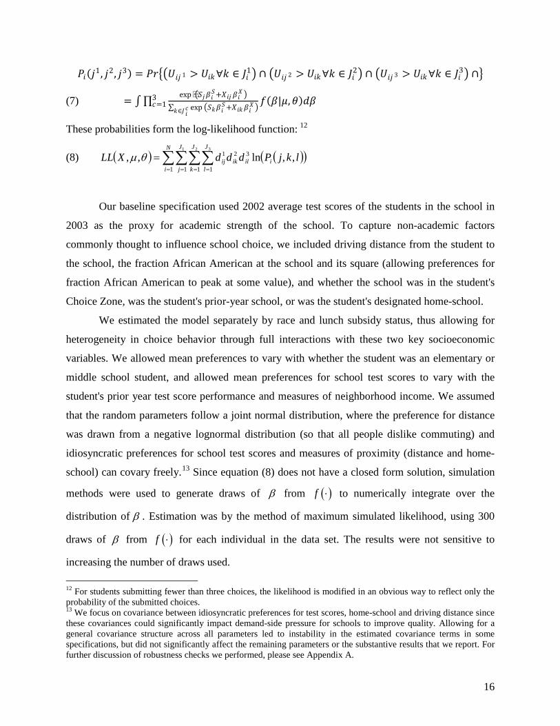
16

𝑃𝑃𝑖𝑖(𝑗𝑗1, 𝑗𝑗2, 𝑗𝑗3) = 𝑃𝑃𝑃𝑃��𝑈𝑈𝑖𝑖𝑗𝑗 1 > 𝑈𝑈𝑖𝑖𝑖𝑖∀𝑖𝑖 ∈ 𝐽𝐽𝑖𝑖1� ∩ �𝑈𝑈𝑖𝑖𝑗𝑗 2 > 𝑈𝑈𝑖𝑖𝑖𝑖∀𝑖𝑖 ∈ 𝐽𝐽𝑖𝑖2� ∩ �𝑈𝑈𝑖𝑖𝑗𝑗 3 > 𝑈𝑈𝑖𝑖𝑖𝑖∀𝑖𝑖 ∈ 𝐽𝐽𝑖𝑖3� ∩�

(7) = ∫∏exp�𝑆𝑆𝑗𝑗𝛽𝛽𝑖𝑖

𝑆𝑆+𝑋𝑋𝑖𝑖𝑗𝑗 𝛽𝛽𝑖𝑖𝑋𝑋 �

∑ exp �𝑆𝑆𝑖𝑖𝛽𝛽𝑖𝑖𝑆𝑆+𝑋𝑋𝑖𝑖𝑖𝑖 𝛽𝛽𝑖𝑖

𝑋𝑋 �𝑖𝑖∈𝐽𝐽 𝑖𝑖𝑐𝑐

3𝑐𝑐=1 𝑓𝑓(𝛽𝛽|𝜇𝜇,𝜃𝜃)𝑑𝑑𝛽𝛽

These probabilities form the log-likelihood function: 12

( ) ( )( )∑∑∑∑= = = =

=N

i

J

j

J

k

J

liilikij lkjPdddXLL

1 1 1 1

3211 2 3

,,ln,, θµ

(8)

Our baseline specification used 2002 average test scores of the students in the school in

2003 as the proxy for academic strength of the school. To capture non-academic factors

commonly thought to influence school choice, we included driving distance from the student to

the school, the fraction African American at the school and its square (allowing preferences for

fraction African American to peak at some value), and whether the school was in the student's

Choice Zone, was the student's prior-year school, or was the student's designated home-school.

We estimated the model separately by race and lunch subsidy status, thus allowing for

heterogeneity in choice behavior through full interactions with these two key socioeconomic

variables. We allowed mean preferences to vary with whether the student was an elementary or

middle school student, and allowed mean preferences for school test scores to vary with the

student's prior year test score performance and measures of neighborhood income. We assumed

that the random parameters follow a joint normal distribution, where the preference for distance

was drawn from a negative lognormal distribution (so that all people dislike commuting) and

idiosyncratic preferences for school test scores and measures of proximity (distance and home-

school) can covary freely.13

β

Since equation (8) does not have a closed form solution, simulation

methods were used to generate draws of from to numerically integrate over the

distribution of . Estimation was by the method of maximum simulated likelihood, using 300

draws of from ( )f ⋅ for each individual in the data set. The results were not sensitive to

increasing the number of draws used. 12 For students submitting fewer than three choices, the likelihood is modified in an obvious way to reflect only the probability of the submitted choices. 13 We focus on covariance between idiosyncratic preferences for test scores, home-school and driving distance since these covariances could significantly impact demand-side pressure for schools to improve quality. Allowing for a general covariance structure across all parameters led to instability in the estimated covariance terms in some specifications, but did not significantly affect the remaining parameters or the substantive results that we report. For further discussion of robustness checks we performed, please see Appendix A.

β ( )f ⋅

β

17

3.2.2 Identification of the Exploded-Mixed-Logit Model

Several aspects of the CMS school choice data help to identify the parameters in our

demand model. First, the large scale redistricting that occurred with the introduction of school

choice helps to identify values placed on distance separately from residential sorting. Residential

sorting could overstate the importance of proximity and neighborhood schools if parents had

previously located near to their preferred schools. However, the former school assignment zones

often required parents to live far from their preferred school, and with large scale redistricting

many parents unexpectedly found themselves assigned to new neighborhood schools. Thus, in

the first year of the choice plan, home-school assignment and distance to a school were not

strongly linked to preferences through prior residential sorting. Multiple choices listed by those

selecting their home-schools first further separates preferences for school characteristics from

residential sorting by simulating the unavailability of the neighborhood school.

Second, historic placement of schools for busing in CMS provides wide variation in

school characteristics for families in all socioeconomic groups, dampening collinearity problems

that may be present in other settings. For example, as was seen in Table I, students from all

socioeconomic groups had high scoring schools within reasonable proximity. Third,

approximately 95 percent of parents submitted choices for the choice plan. Thus we have data for

nearly the entire student population—whereas most work using school choice data has been

dependent on limited and potentially non-representative subgroups of students.

Fourth, the multiple-ranked responses provided by each parent creates variation in the

choice set by effectively removing the prior chosen school from the subsequent choice set. This

choice-set variation allows us to estimate the distribution of values parents place on school

characteristics from observed substitution patterns for each individual – a stronger source of

variation for identification than cross-sectional changes in the choice set based on geographic

location (Train (2003), Berry, Levinsohn, and Pakes (2004)). Intuitively, when only a single

(first) choice is observed for every individual, it is difficult to be sure whether an unexpected

choice was the result of an unusual error term ( ijε ) or an unusually high weight placed by the

individual on some aspect of the choice ( ). However, when an individual makes multiple

choices that share a common attribute (e.g., high test scores) we can infer that the individual has

a strong preference for that attribute, because independence of the additive error terms across

choices would make observing such an event very unlikely in the absence of a strong preference.

iβ

18

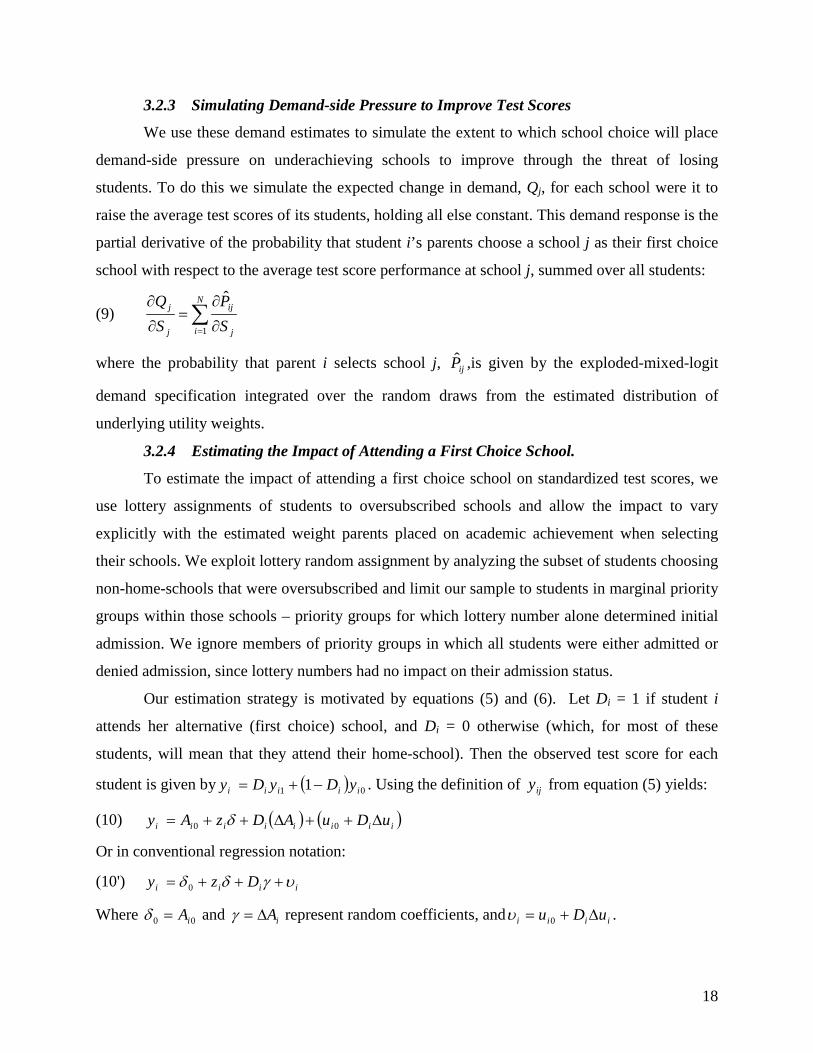
3.2.3 Simulating Demand-side Pressure to Improve Test Scores

We use these demand estimates to simulate the extent to which school choice will place

demand-side pressure on underachieving schools to improve through the threat of losing

students. To do this we simulate the expected change in demand, Qj, for each school were it to

raise the average test scores of its students, holding all else constant. This demand response is the

partial derivative of the probability that student i’s parents choose a school j as their first choice

school with respect to the average test score performance at school j, summed over all students:

(9) ∑= ∂

∂=

∂

∂ N

i j

ij

j

j

SP

SQ

1

ˆ

where the probability that parent i selects school j, ijP̂ ,is given by the exploded-mixed-logit

demand specification integrated over the random draws from the estimated distribution of

underlying utility weights.

3.2.4 Estimating the Impact of Attending a First Choice School.

To estimate the impact of attending a first choice school on standardized test scores, we

use lottery assignments of students to oversubscribed schools and allow the impact to vary

explicitly with the estimated weight parents placed on academic achievement when selecting

their schools. We exploit lottery random assignment by analyzing the subset of students choosing

non-home-schools that were oversubscribed and limit our sample to students in marginal priority

groups within those schools – priority groups for which lottery number alone determined initial

admission. We ignore members of priority groups in which all students were either admitted or

denied admission, since lottery numbers had no impact on their admission status.

Our estimation strategy is motivated by equations (5) and (6). Let Di = 1 if student i

attends her alternative (first choice) school, and Di = 0 otherwise (which, for most of these

students, will mean that they attend their home-school). Then the observed test score for each

student is given by ( ) 01 1 iiiii yDyDy −+= . Using the definition of ijy from equation (5) yields:

(10) ( ) ( )iiiiiiii uDuADzAy ∆++∆++= 00 δ

Or in conventional regression notation:

(10') iiii Dzy υγδδ +++= 0

Where 00 iA=δ and iA∆=γ represent random coefficients, and iiii uDu ∆+= 0υ .

19

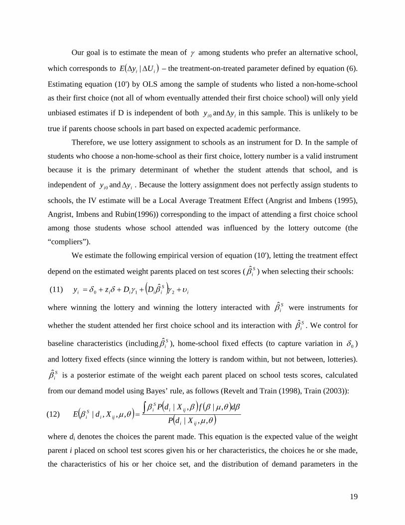
Our goal is to estimate the mean of γ among students who prefer an alternative school,

which corresponds to ( )ii UyE ∆∆ | – the treatment-on-treated parameter defined by equation (6).

Estimating equation (10') by OLS among the sample of students who listed a non-home-school

as their first choice (not all of whom eventually attended their first choice school) will only yield

unbiased estimates if D is independent of both 0iy and iy∆ in this sample. This is unlikely to be

true if parents choose schools in part based on expected academic performance.

Therefore, we use lottery assignment to schools as an instrument for D. In the sample of

students who choose a non-home-school as their first choice, lottery number is a valid instrument

because it is the primary determinant of whether the student attends that school, and is

independent of 0iy and iy∆ . Because the lottery assignment does not perfectly assign students to

schools, the IV estimate will be a Local Average Treatment Effect (Angrist and Imbens (1995),

Angrist, Imbens and Rubin(1996)) corresponding to the impact of attending a first choice school

among those students whose school attended was influenced by the lottery outcome (the

“compliers”).

We estimate the following empirical version of equation (10'), letting the treatment effect

depend on the estimated weight parents placed on test scores ( Siβ̂ ) when selecting their schools:

(11) ( ) iSiiiii DDzy υγβγδδ ++++= 210

ˆ

where winning the lottery and winning the lottery interacted with Siβ̂ were instruments for

whether the student attended her first choice school and its interaction with Siβ̂ . We control for

baseline characteristics (including Siβ̂ ), home-school fixed effects (to capture variation in 0δ )

and lottery fixed effects (since winning the lottery is random within, but not between, lotteries). Siβ̂ is a posterior estimate of the weight each parent placed on school tests scores, calculated

from our demand model using Bayes’ rule, as follows (Revelt and Train (1998), Train (2003)):

( ) ( ) ( )( )θµ

βθµβββθµβ

,,|

,|,|,,,|

iji

ijiSi

ijiSi XdP

dfXdPXdE ∫=

where di denotes the choices the parent made. This equation is the expected value of the weight

parent i placed on school test scores given his or her characteristics, the choices he or she made,

the characteristics of his or her choice set, and the distribution of demand parameters in the

(12)

20

population. We calculate this posterior for each student in our randomized lottery admission

group using 1,000 draws from the estimated demand parameter distribution.14

Siβ̂

Note that incorporates all information about a parent’s choices and the tradeoffs she

faced into one index summarizing the importance of school test scores in determining that

parent’s school choice. In addition, it depends only on baseline data that is independent of

whether the student won the lottery, so its interaction with winning the lottery is therefore a valid

instrument once one has conditioned on baseline data. Finally, note that coefficient estimates for

terms involving Siβ̂ are not attenuated by the usual measurement error bias because the

measurement error ( Si

Si ββ ˆ− ) is uncorrelated with the posterior estimate S

iβ̂ by construction

(Hyslop and Imbens (2001)).

4. Data and Empirical Results

4.1 Data

We obtained secure access to administrative data for all students in CMS for the year

before and after the implementation of school choice. Throughout the analysis, we focus on

students entering grades four through eight because of the lack of test scores (either baseline or

outcome) for other grades. Students take End of Grade tests in grades three through eight, so that

students entering grade four are the first to have a baseline test available.

For each student, we have the choice forms submitted to CMS, allowing each parent to

specify up to three choices for her child’s school. In addition to the parental choices our data

contain student characteristics for the years before and after school choice, including geocoded

residential location, race, gender, lunch subsidy recipient status, and school assignment. Student

test scores are for North Carolina End of Grade Exams in math and reading, and were

standardized to be mean zero and standard deviation one in each grade and year. These tests

were developed specifically by North Carolina to measure student progress, and were aligned to

measure progress on a single underlying factor across all grades (Sanford (1996)). We use these

data to construct key covariates in the demand for schools, such as driving distance from each

14 See Train (2003) p. 270 for Monte Carlo simulations of the accuracy of individual-level parameter estimates and the number of observed choice situations.

21

student to each school, an indicator for busing availability, an indicator for the prior-year’s

school, measures of student-level income, student baseline academic achievement, school-level

academic achievement, and school-level racial composition. The variables used in our model are

described in detail in Table II.

The final estimation sample used to estimate the exploded-mixed-logit model included

36,887 students entering grades four through eight. The means and standard deviations of these

variables across the 2.4 million school, student, and choice rank combinations used to estimate

the model are reported in columns 1 and 2 of Table III, and the mean and standard deviation of

the average characteristic across students is reported for the 36,887 students are reported in

columns 3 and 4.

4.2 Empirical Results

Table IV presents the results from the exploded-mixed-logit demand estimation in four

subsamples, defined by race and lunch recipient status. We report the estimates for the mean of

each logit coefficient, along with the standard deviations and correlations (where appropriate) for

the random parameter distributions. The parameters determining the importance of school test

scores in school choice are reported at the top of Table IV, followed by the parameters that

govern the distribution of preferences for non-academic factors. We allowed the mean of each

logit coefficient to vary by grade level (elementary versus middle school student), and we further

allowed the mean weight that a parent placed on school test scores to depend on the student’s

own baseline test score and neighborhood income (i.e., interaction terms with school test scores).

Baseline test scores and neighborhood income (in thousands) are constructed as deviations from

the average, so that the coefficient on school scores represents the weight placed on test scores

for a student with average test scores and neighborhood income (when the interactions are zero).

The standard errors for each of the estimates are reported in Appendix Table B.I. All of the

parameters were precisely estimated and statistically significant.

Broadly speaking, the estimates are consistent with expectations. Focusing first on the

means of the coefficients, parents of both elementary and middle school students in all four

subsamples were less likely to choose a school far away, and more likely to choose a school that

22

had high test scores, was their home-school15

In addition to the variation related to observable characteristics, idiosyncratic preferences

contributed substantial variation to the weight placed on both academic and non-academic

factors, with the estimated standard deviation for most of the random coefficients ranging

between one-quarter and one-half of the mean for each coefficient. The variation arising from

idiosyncratic preferences for school scores was similar in magnitude to the variation arising from

neighborhood income and baseline scores. A one standard deviation increase in the random

coefficient raised the weight placed on school scores by 0.2 to 0.7 across the four subsamples,

while a one standard deviation increase in neighborhood income (about $25 thousand) raised the

weight placed on school scores by 0.1 to 0.4, and a one standard deviation increase in student

baseline test score raised the weight placed on school scores by 0.2 to 0.6. For all four

subsamples, the random coefficient on school scores was negatively correlated with the random

coefficient on home-school and positively correlated with the random coefficient on distance.

, had a majority of students their own race, was

their school in the prior year, or was a school in their choice zone (assuring school bus

transportation). The average middle school parent placed relatively less weight on non-academic

factors (distance, attending last year’s school, and attending a school in the choice zone) and

relatively more weight on academic factors (school test scores) than did the average elementary

school parent, implying that parents of middle school students were more responsive to test score

differences all else equal (as one might expect).

Among both elementary and middle school parents, the estimates in Table IV suggest

substantial heterogeneity in the weight placed on academic versus non-academic factors. The

positive interactions with school score indicate that the average weight placed on school score

increased with both neighborhood income and the student’s baseline test score for parents of

students in all four subgroups. Holding neighborhood income and baseline test scores constant,

non-whites placed more weight on school scores than whites, while parents of students not

receiving lunch subsidies placed more weight on school scores than those receiving lunch

subsidies. Relative to parents of white students, parents of non-white students preferred schools

in which a larger fraction of students were black, but otherwise tended to place less weight on the

non-academic factors.

15 The home-school preference could be consistent with a default effect, rather than a preference for a neighborhood school, since the home-school was listed as the default option. Hastings et al. (2007a) provide evidence suggesting that preference for a home-school represents a neighborhood preference rather than default behavior.

23

Hence parents who consider options outside of their home-schools are more likely looking for

high test scores when deciding which schools to pick. For the average parent, selecting a high-

achieving school will require her to choose a school that is farther than her home-school and a

school that is not the home-school, leading to tradeoffs between academic gains and proximity.

One way to interpret the magnitude of the coefficients and the amount of heterogeneity

reported in Table IV is in relative terms. For example, the ratio of the mean school score

coefficient to the mean distance coefficient for white, non-lunch, elementary students implies

that the average parent would be willing to travel an additional 3.8 miles to attend a school with

one standard deviation test scores. Within this subsample, variation in neighborhood income,

student baseline score, and the random coefficients for school score and distance each generate a

standard deviation across parents of about one to two miles in the willingness to travel to attend a

high score school. Parallel calculations suggest a similar amount of variation between the

subsamples, and within each subsample, in the tradeoffs parents are willing to make. Another

way to interpret the magnitude of the coefficients is to calculate what they imply for the

probability of choosing an alternative school, relative to the home-school (the odds ratio). The

mean school score coefficient for white, non-lunch, elementary students implies that a one

standard deviation increase in school scores at the alternative school will increase the odds of

choosing that school by 331 percent (e1.46-1). The increase in the odds of choosing the alternative

school would be considerably larger for a parent whose coefficient on school scores was one

standard deviation above the mean (e1.46+0.402-1 = 544 percent). Looking ahead, this substantial

variation across students in the weight placed on academics suggests that we may expect to see

strong school choice selection on academic outcomes for some students and not for others. The

fact that much of the heterogeneity in preferences is unobservable implies that the traditional

approach of allowing the treatment effect to vary with observable characteristics, such as race or

lunch status, may not completely capture heterogeneous preferences for academics.

In addition to trading-off proximity for academics, African American parents must

tradeoff academic gains against the racial composition of peers. The coefficients on percent

black and its square imply that the average African American parent prefers majority black

schools, while the average white parent prefers schools that are majority white. The racial

preferences are stronger for elementary school students than for middle school students in three

of the subsamples, although it may be that racial preferences near endpoints are difficult to

24

estimate precisely since there are few schools (particularly middle schools) that are near 100

percent of either race. The coefficients in Table IV imply that the average parent of an African

American student is 10-70 percent less likely to choose a school that is 35 percent black versus a

school that is 80 percent black, all else equal, whereas the average parent of a white student is

two to three times more likely to select the low-minority school. In CMS, the percent black at a

school is negatively correlated with average test scores, implying that African American parents

must value academic achievement more than their white counterparts in order to induce them to

choose a higher performing school that also has, on average, fewer African American students.

4.3 Robustness Checks for Demand Model

We conducted several robustness checks of the exploded-mixed-logit model.16

Second, due to the way the lottery was run, parents may have had an incentive to

misrepresent their true preferences. If they understood the allocation mechanism, a parent with

an undesirable home-school might want to hedge against being assigned to the home-school.

They would do so by picking less desirable schools than they actually prefer – trading off

First, we

estimated the model using alternative measures of a school’s academic performance. Given the

major policy change under the choice plan, parents may have had a difficult time predicting

expected academic performance at schools in their choice set, and may have used indicators of

school performance other than the measure we used in our baseline model. Our baseline

specification used average 2002 test scores of the students in the school in 2003. But we also

estimated models using average 2003 test scores of the students in the school in 2003, average

2002 scores for students in each school in 2002, and a “value added” measure of each school’s

impact on academic achievement in the prior year (estimated as the school fixed effect from a

regression of End of Grade test score on prior year test score and other student baseline

characteristics, such as race, gender, and subsidized lunch status). The parameter estimates

across the three measures of average test scores were quite similar, but the model using our base

specification had the highest likelihood value, and in that sense fit the choice data best. We found

that the model using value added did not fit the observed choice data well at all. This should not

be surprising, since school value added estimates were not available to parents in 2002.

16 See Hastings, Kane and Staiger (2007a) for details. The key findings are reproduced in Appendix A for convenience.

25

desirability for increased chance of being admitted. However, as discussed earlier, it was not at

all clear that parents had the information or experience in the first year of choice to understand

how to exploit the incentives of the allocation mechanism. We tested for the presence of strategic

behavior in the first year of choice by exploiting the redrawing of school boundaries. Many of

those who lived in the same contiguous school assignment zone in 2001-2002 were given

different home-school assignments in 2002-2003. Hence, among those with the same school

assignments who lived in the same neighborhood in 2001-2002, some students experienced

positive and others negative shocks to the quality of their guaranteed school. If strategy was a

major component of parental choices, we would expect to see very different choice behavior for

those with negative versus positive shocks to the quality of their home-school. We did not,

however, find significant differences in the exploded-logit parameters (particularly for the

coefficients relating to school test scores) across families experiencing positive and negative

shocks to their guaranteed school within the subsample of students who lived in 2001-2002

assignment zones that were split by redistricting. This suggests that strategy was not a major

factor driving our demand estimates in this first year of the public school choice plan.

Finally, we used the exogenous reassignment of nearly half of the students in the district

to test the extent to which residential sorting affected our demand estimates. Residential sorting

could lead us to overstate preferences for proximity if parents had already sorted to live next to

the schools they preferred. To test for the potential effects of residential sorting on our estimates,

we re-estimated our model for the subsample of students who were reassigned (whose school

assignments under the busing plan in 2001-2002 were different from their home-school in 2002-

2003). The estimated parameters were qualitatively and quantitatively similar in the reassigned

subsample compared to those for the full sample, suggesting that endogenous residential location

is not a major source of bias in this data. The similarity of the results is not surprising because

our model is using the information in multiple choices to identify preferences. A substantial

fraction of parents who listed their home-school also listed subsequent choices. For these

parents, multiple choices simulate reassignment whether or not they were actually reassigned.

4.4 Implications for Demand-side Pressure to Improve Academic Achievement

The exploded-mixed-logit estimates can be used to simulate the degree to which demand-

side pressure for academic improvement varied across low-and high-performing schools under

26

public school choice. To examine the extent to which public school choice affects the demand

for each school, we took each school individually, added 0.34 average student-level standard

deviations to its mean school score, holding all else equal, and simulated the change in the

number of students listing that school as a first choice.17 The simulated change in demand tells

us how responsive each school’s demand curve is with respect to their own test score

outcomes.18

Figure 3 plots differences in average baseline test scores (in 2002) between the marginal

students (those who are drawn in by the .34 average student-level standard deviation score

increase) and students who previously enrolled in each school. The incentive for any school to

Figure 2 plots the change in number of students listing a school as a first choice by the

school’s original average score (each point in the figure is the result of a simulation for a

different school). Because of the difference in size, we plot the results separately for elementary

(Figure 2a) and middle (Figure 2b) schools. The demand response is quite different for schools

that were originally high and low scoring. The upward sloping relationship implies that the

demand response is greatest among schools that were already high scoring. This result reflects

the parameter estimates in the exploded-mixed-logit model. Parents with high preferences for

school scores, and thus low preferences for their neighborhood schools, are sensitive to changes

in school scores and are willing to consider a broader set of schools beyond their home-school.

These parents are likely to only consider high scoring schools for their children and are willing to

change schools in response to an increase in score at another high scoring school, even one that

is located further away. This pattern is substantially stronger for middle schools, reflecting the

fact that parents of middle school students tend to place higher weights on test scores and lower

(less negative) weights on distance than elementary school parents do. The results imply that the

demand-side incentives to focus on student performance are larger for higher-performing

schools, since these schools compete more intensely on academic quality for the quality-elastic

segment of the population, and this disparity in demand-side pressure is particularly strong for

middle schools when compared to elementary schools.

17 This is approximately equivalent to a 10 point increase in the average percentile score for students attending that school. 18 As a check on the model fit, we compared the predicted demand based on observed school characteristics with the actual number of students who listed each school choice first and found that the predicted and actual demand was correlated 0.91 across schools. A regression line of actual demand on predicted demand had a coefficient of 0.954 that is not statistically different from one.

27

improve its performance would be dampened if, in doing so, they were swamped by lower-

performing students, who would bring down mean performance and potentially be more costly to

educate. The fact that most points lie above the 45 degree line implies that the marginal students,

on average, were higher performing than the students already enrolled. Again, this reflects the

heterogeneity that was estimated in the exploded-mixed logit model, with higher performing

students placing the highest weight on school test scores in choosing a school.

The key features of the simulations reported in Figures 2 and 3 appear to be driven

primarily by the estimated heterogeneity in preferences, rather than other details of the

specification. We found similar results in all the alternative specifications we have estimated that

allowed for heterogeneity in preferences.19

As outlined in Section 3, heterogeneous choice behavior across families may have

immediate impacts on academic achievement for students of parents exercising choice. To

estimate the effect of attending a first choice school and how it relates to the importance placed

on academics when selecting a school, we analyzed the subset of students choosing schools that

were oversubscribed and limited our sample to students in marginal priority groups within those

schools – priority groups for which lottery number alone determined initial admission. We ignore

members of priority groups in which all students were either admitted or denied admission –

The results imply that instead of increasing pressure

on low-performing schools to improve through the threat of losing students, high-performing

schools will face the most pressure to improve because they serve high-performing students

whose parents are willing to switch schools in response to small changes in test scores. Thus,

school choice is likely to generate changes in demand that act to widen rather than narrow the

gap between high- and low-performing schools. We next turn to examine the implications of

heterogeneous choice behavior for the immediate impact of allowing parents to send their

children to the school of their choice.

4.5 Heterogeneous Treatment Effect from Attending a First Choice School

19 For example, estimates from an exploded-logit model without random coefficients (but otherwise flexibly specified as in Table 4) yielded similar simulation results and similar (though less precise) estimates of how the impact of attending a first choice school varied with the weight placed on school test scores. Because we used individual-level data with multiple responses and wide variation in the choice set, we could specify the model very flexibly and identify significant heterogeneity in preferences even without the random coefficients through interactions with observable characteristics.

28

since the assignment of lottery numbers had no impact on their admission status. This allows us

to use the random admission of students into a school, conditional on the school they chose, as

an instrument for attending a first choice school.20

Table V compares baseline characteristics of students in the marginal priority group to

other students in the district. Overall, students in the marginal priority group appear to be fairly

representative of students who chose a non-guaranteed school. The only notable differences are

that students in the marginal priority group were more likely to be eligible for lunch subsidies

than students in the waitlisted group (reflecting the priority given to eligible students), and they

applied to schools with higher test scores than did students in the admitted group (reflecting

capacity constraints at schools with higher test scores). Not surprisingly, students choosing non-

guaranteed schools differed from students who chose a guaranteed school: they had home-

schools with lower test scores and higher proportions of minority and lunch-eligible students,

and were more likely to be minority, poor, and doing poorly in school themselves. Thus, the

marginal priority group should provide a reasonable estimate of the impact of attending one’s

first choice school for a typical student who chose a non-guaranteed school (i.e., treatment on the

treated). In addition, the final row in Table V shows the mean weight placed on school scores (

We began with a sample of 37,115 students entering grades four through eight. Of these,

22,872 listed their guaranteed home-school (n=19,669) or magnet continuation school (n=3,203)

and, therefore, were not subject to randomization. Another 7,583 students were in groups

sufficiently high on the priority list that they were not subject to the randomization. There were

3,065 students in marginal priority groups, described above as those priority groups within the

schools where slots were allocated on the basis of a random number. Finally, there were 3,595

students in priority groups that were sufficiently low on the priority list that all members of the

priority group were denied admission and placed on the waitlist.

Siβ̂ ) for students in the marginal priority group versus other students in the district, calculated by

20 In some schools, the marginal priority group will consist of those who attended the school the year before, free-or reduced-lunch eligible students, or students from the choice zone. The marginal priority group may also be different for different grade levels in a school.

29

equation (8). The mean Siβ̂ for students in the randomized group is very similar to that for

students in the district as a whole.21

The first panel reports the adjusted difference between lottery winners and losers for

various baseline characteristics. None of the coefficients are significant, confirming that winning

the lottery was independent of baseline characteristics, as would be expected if it was randomly

assigned within the marginal priority groups. The second panel of Table VI tests for differences

in attrition, using presence in CMS at the end of the 2002-2003 school year as the dependent

variable. The results show no evidence of differential attrition across lottery winners and

losers.

Table VI verifies the lottery randomization and examines the impact winning the lottery

had on characteristics of the attended school in the 2002-2003 school year. For the experiment to

be valid, baseline characteristics should be balanced across lottery winners and losers,

differential attrition should be minimal, and winning the lottery should significantly increase the

probability of attending a first choice school. The adjusted difference reported in Table VI is the

estimated impact of winning the lottery on each of these outcomes, from a regression that

included school lottery fixed effects to focus on differences within lottery and account for the

fact that the probabilities of winning the lottery varied across lotteries (Rouse 1998). Our

estimation sample excludes 181 students who were in marginal priority groups but missing

needed baseline characteristics, such as address (which was used in the choice model).

22

21 The low mean weight for students in the admitted group is consistent with the fact that these students were typically choosing lower-scoring and capacity unconstrained schools, as can be seen from the differences in sample means for the Average Combined Scores of the chosen school (row 8 in Table V). 22 Average attrition rates were fairly low at 9.8 percent and consistent with estimates of inter-county mobility rates from the Census.

The third panel of Table VI shows the impact of winning the lottery on the

characteristics of the school attended at the end of the 2002-2003 school year. Lottery winners

were 53 percentage points more likely to attend the first choice school than the lottery losers.

This estimate is not equal to 100 percent for two reasons: first, some of those who were given the

opportunity to attend the first choice did not do so, and second, some of those who were

originally waitlisted at the first choice school were subsequently called off the waitlist. Students

who won the lottery attended schools with approximately one-tenth of a student-level standard

deviation higher test scores. Thus winning the lottery appears to be a valid instrument for

30

attending a first choice school and significantly increased the test score of the school students

attend.

To test the empirical implications of the model derived Section 3, we estimated the

impact of attending a first choice school on a student’s test score using equation (11):

(11) ( ) iSiiiii DDzy υγβγδδ ++++= 210

ˆ

where winning the lottery and its interaction with Siβ̂ (the estimate weight each parent placed on

school test scores) were instruments for attending a first choice school (Di) and its interaction

with Siβ̂ . We control for baseline characteristics (to capture zi), home-school fixed effects (to

capture variation in 0δ ) and lottery fixed effects (since winning the lottery is random within, but

not between lotteries). Baseline characteristics included Siβ̂ , measures of student performance

from the prior year (math and reading score, had more than 18 absences, was suspended, was

retained) and measures of student demographics (neighborhood income, African American, other

minority, female, received lunch subsidy).23

Siβ̂

We did not correct the standard errors of our IV

regressions for the presence of a generated regressor, because the estimation error in (due to

estimation error in the underlying parameters in the exploded-mixed-logit model) was less than 1

percent.

Table VII presents the results from estimating (11) by instrumental variables, using

student combined average test score at the end of the 2002-2003 school year as the dependent

variable. The key prediction from Section 3 was that the coefficient on the interaction should be

positive ( 02 >γ ). The first two columns present results for all students, with and without the

interaction between attending a first choice school and Siβ̂ . The first column shows no significant

average impact of attending a first choice school on own test score, similar to average treatment

effects in prior studies (Cullen, Jacob, and Levitt (2006)). The point estimate is very close to zero

(-0.005) and has a large standard error (0.050). The second column shows that the weight parents

placed on school scores ( Siβ̂ ) when selecting schools is a significant and positive determinant of

how attending a first choice school affects test score outcomes. The regression estimates imply

23 We do not report the coefficients on the baseline covariates, but the largest determinants of test scores was baseline test scores. Female was the only other student-level demographic characteristics that was consistently significant, and was positively associated with test scores.

31

that a one standard deviation increase (0.81) in the weight that an individual places on school test

scores raises the treatment effect on the student’s own test score by 0.066 standard deviations.

For parents who placed no weight on test scores in their school choices, the coefficient on

attending the first choice school implies a negative (although not significant) treatment effect –

the students’ test scores fall by 0.143 standard deviations if they attend the first choice school.

These estimates imply a near zero impact (0.002 standard deviation score gain) of attending a

first choice school on test scores for an average student with a Siβ̂ of 1.79, and a large positive

effect on test scores (about 0.10) for students at the 95th percentile of the Siβ̂ distribution. A 0.1

standard deviation increase in a student’s test score results is equivalent to a three to four

percentile rank gain in test scores. Estimates of the impact that test scores have on future

earnings suggest that a 0.1 standard deviation in increase in test scores is worth $10,000 to

$20,000 in net present value of future earnings (Kane and Staiger (2002)).24

The second general prediction from our model is that if

Siβ̂ is low because parents place

low weight on a school’s contribution to their child’s achievement (as opposed to because school

test scores are unrelated to their child’s achievement), then the impact of attending a first choice

school will depend on how other valued school characteristics are related to the academic quality

of the school. To test this prediction, the last four columns of Table VII show estimates for two

subgroups of parents: those for whom the estimated preferred percent minority at a school is less

than 50 percent (primarily white students) and those for whom it is greater than 50 percent

(primarily black students).25

Siβ̂

Since school test scores are negatively correlated with percent

minority in a school, parents who prefer a school with a high proportion of African American

students will tend to choose lower performing schools unless they place a high weight on school

scores. In contrast, parents that prefer schools with a low proportion of African American

students will tend to choose high performing schools regardless of the weight they place on

school scores. In other words, the interaction effect between and attending a first choice

24 There is some evidence that students may experience a drop in test scores from switching schools, particularly moving from elementary to middle schools. (Cook et al. (2006), Rockoff and Lockwood (2009)). We estimate our main regression specification separately for rising-grade and non-rising-grade students (rising sixth graders versus all others), and find some evidence of an adverse mean impact of matriculating to middle school but overall the pattern of results are similar across the two subgroups. 25 Posterior estimates of preferences for school racial composition were calculated in the same way as the S

iβ̂ s.

32

school should have a negative intercept and a steeper slope for students who have strong

preferences for predominantly African American schools.

Columns 3 and 4 show that the average treatment effect is positive for students whose

parents prefer a predominantly white school, and there is no significant interaction with the

weight that the parent places on test scores in their school choice. Among students of parents

who prefer predominantly white schools, both relatively high- and low- Siβ̂ students experienced

academic gains from attending the first choice school. In contrast, columns 5 and 6 indicate that

students of parents who prefer a predominantly black school have a significant interaction

between the estimated preference for academics and the treatment effect. High- Siβ̂ students

experienced academic gains from attending the first choice school that are similar to students

whose parents prefer a predominantly white school. In contrast, low- Siβ̂ students with parents

that prefer a predominantly black school experience a negative effect on academic performance

from attending the first choice school.

These results suggest that heterogeneity in the relative importance parents place on

academics when choosing schools and the tradeoffs they face in their choice sets are both

important determinants of the immediate gains from school choice. They imply that public

school choice may have a negative impact on the academic achievement of the students it is most

intended to help – minority students from disadvantaged backgrounds. The results in Table VII

suggest that, on average, school choice widens rather than narrows the gap in achievement

between low- and high-SES families exercising choice.

Not only do measures of parental choice behavior explain heterogeneous impacts from

attending a first choice school, but they also highlight why subgroup impacts examined in prior

studies vary through correlation between demographics and choice behavior. Table VIII shows

estimates of the average treatment effect on student test scores in various subgroups of students

defined on the basis of student demographics or characteristics of the school chosen. Prior

studies have used these subgroups of students who on a priori grounds may have different

underlying reasons for choosing schools that may be correlated with the expected treatment

effect. Estimates for most of the subgroups remain insignificant. However, the estimated

treatment effect is positive and significant for two of the subgroups (whites and students with

above median income) and there is an apparent pattern of positive treatment effects for higher

33

SES students and students applying to higher-scoring schools. The pattern of subgroup impacts is

strongly related to the average weight ( Siβ̂ ) that parents place on school test scores. Column 2 of

Table VIII reports the mean of Siβ̂ for students in each of the subgroups, and Figure 4 plots this

mean against the subgroup estimates from column 1. The strong positive correlation between the

two (correlation=0.89) suggests that differences in impacts across subgroups may be generated

by differences in the underlying determinants of choice. Moreover, the large variation in Siβ̂

within each subgroup reported in column 3 of Table VIII suggests that any of these simple

subgroup impacts will capture only a fraction of the heterogeneity in outcomes if differences in

the weights parents place on academics are driving heterogeneous treatment effects.

This evidence highlights three advantages of using demand estimates to identify

heterogeneous treatment effects versus subgroup estimation based on observables, such as race

and income. First, using a single index, rather than estimating differences in impacts for an

arbitrary number of subgroups, increases the precision with which we can identify heterogeneous

treatment effects by exploiting all of the within- and between-subgroup variation in preferences.

Second, the Siβ̂ incorporate information on parental rankings and the choice set they faced,

distinguishing between students who pick a school because it is convenient versus students who

repeatedly pick less convenient schools for academics reasons. Third, the demand estimates give

us an economic interpretation of subgroup impacts, allowing us to evaluate the impact of school

choice outside of the estimation sample, and to potentially redesign school choice plans to

address differences in the underlying drivers of parental choice (Hastings and Weinstein (2008)).

5. Conclusion

One of the most important goals of public school choice plans is to increase academic

performance for disadvantaged students by allowing them to attend higher-performing schools

and by creating pressure on failing schools to improve through the threat of losing students. Both

of these goals require that parents value academics and choose schools accordingly when offered

the opportunity to do so. This paper departs from the prior empirical literature on public school

choice by combining rich choice data, lottery assignments, and student outcomes to examine the

34

implications that heterogeneous choice behavior had for equity and quality of educational

opportunities for disadvantaged families.

We find that heterogeneity in the weights parents place on school test scores drive both

demand-side pressure for schools to improve and immediate academic gains from attending an

alternative school. Because low-SES families place less emphasis on academics when choosing

schools, the school choice plan led to high demand response for high-performing schools serving

high-SES families and little demand response for low-performing schools serving local, low-SES

families. Thus, the demand response under public school choice would tend to increase

education stratification in Charlotte rather than produce a competitive tide that lifts all boats. At

the same time, allowing parents to choose an alternative school led to worse academic outcomes

for many children of disadvantaged minority families who had to trade off academic strength of

the school to attend a predominantly black school, but better academic outcomes for white

children who faced no such tradeoff. Therefore, school choice widened rather than narrowed the

gap in achievement between low- and high-SES families exercising choice.

Finally, understanding the economic underpinnings of heterogeneous treatment effects

and heterogeneous pressures to improve academics can point us towards simple changes in

public school choice design that may increase efficacy in providing greater equity and quality in

public education. In general, the impact of school choice on academic outcomes will depend on

both the willingness of parents to make tradeoffs and the extent to which the available school

choices require such tradeoffs to be made. In other school districts, where parents face less stark

tradeoffs or focus more on academic differences between schools, the outcomes of choice could

be very different. Moreover, interventions such as changing the information set provided to low-

income families (Hastings and Weinstein (2008)) or the strategic placement of schools may

increase demand-elasticity among low-SES families and minimize the tradeoffs they face,

allowing them to share in the potential benefits from public school choice.

35

References Abdulkadiroğlu, Atila, Parag A. Pathak, Alvin E. Roth, and Tayfun Sönmez (2006): “Changing

the Boston School Choice Mechanism: Strategy-proofness as Equal Access,” Working Paper 11965, NBER.

Abdulkadiroğlu, Atila, and Tayfun Sönmez (2003): “School Choice: A Mechanism Design

Approach,” American Economic Review, 93, 729-747. Anderson, Simon P., André de Palma, and Jacques-François Thisse (1992): Discrete Choice

Theory of Product Differentiation. Cambridge, MA: MIT Press. Angrist, Joshua and Guido Imbens (1995): “Two-Stage Least Squares Estimation of Average

Causal Effects in Models with Variable Treatment Intensity,” Journal of the American Statistical Association, 90, 431-442.

Angrist, Joshua, Guido Imbens and Donald Rubin (1996): “Identification of Causal Effects

Using Instrumental Variables”, Journal of the American Statistical Association, 91, 444-472.

Armor, David J. and Peiser, B.M. (1998): “Interdistrict Choice in Massachusetts,” in Learning

from School Choice, ed. by Paul Peterson and Bryan Hassel. Washington, DC: Brookings Institution Press, 157-185.

Ballou, Dale (2007): “Magnet Schools and Peers: Effects on Student Achievement,” Working

Paper, Vanderbilt University. Bayer, Patrick, Fernando Ferreira and Robert McMillan (2004): “Tiebout Sorting, Social

Multipliers and the Demand for School Quality,” Working Paper 10871, NBER. Belfield, Clive R., and Henry M. Levin (2002): “The Effects of Competition Between Schools on

Educational Outcomes: A Review for the United States,” Review of Educational Research, 72, 279-341.

Berry, Steven, James Levinsohn, and Ariel Pakes (2004): “Differentiated Products Demand

Systems from a Combination of Micro and Macro Data: The New Car Market,” Journal of Political Economy, 112, 68-105.

Betts, Julian R., Lorien A. Rice, Andrew C. Zau, Y. Emily Tang, and Cory R. Koedel (2006):

Does School Choice Work? Effects on Student Integration and Achievement. San Francisco, CA: Public Policy Institute of California.

Borland, Melvin V., and Roy M. Howsen (1992): “Students’ Academic Achievement and the Degree of Market Concentration in Education,” Economics of Education Review, 11, 31-39.

36

Borghans, Lex, Angela Lee Duckworth, James J. Heckman and Bas ter Weel (2009): “The

Economics and Psychology of Personality Traits,” Journal of Human Resources. 43: 972-1059.

Cook, Philip J., Robert MacCoun, Clara Muschkin and Jacob Vigdor (2006): “Should Sixth

Grade be in Elementary or Middle School? An Analysis of Grade Configuration and Student Behavior,” Working Paper 12471, NBER.

Cullen, Julie Berry, Brian A. Jacob, and Steven Levitt (2006): “The Effect of School Choice on

Student Outcomes: Evidence from Randomized Lotteries,” Econometrica, 74, 1191-1230.

Dagsvik, John K. (1994): “Discrete and Continuous Choice, Max-Stable Processes, and

Independence from Irrelevant Attributes,” Econometrica, 62, 1179-1205. Della Vigna, Stefano (2009): “Psychology and Economics: Evidence from the Field,” Journal of

Economic Literature, (Forthcoming). Epple, Dennis and Richard Romano (1998): “Competition Between Private and Public Schools,

Vouchers, and Peer-Group Effects.” American Economic Review, 88: 33-62. Epple, Dennis and Richard Romano (2002): “Educational Vouchers and Cream Skimming,”

Working Paper 9354, NBER. Farrell, Joseph and Carl Shapiro (1990): “Horizontal Mergers: An Equilibrium Analysis,”

American Economic Review, 80, 107-126. Glazerman, Steven (1997): “Determinants and Consequences of Parental School Choice”

Unpublished Working Paper, University of Chicago, Harris School of Public Policy. Glazerman, Steven, and Robert H. Meyer (1995): “Public School Choice in Minneapolis” in

Midwest Approaches to School Reform: Proceedings of a Conference Held at the Federal Reserve Bank of Chicago October 26-27, 1994, ed. by Thomas A. Downes, and William A. Testa. Chicago, IL: Federal Reserve Bank of Chicago, 110-126.

Greene, Jay P., Paul E. Peterson, and Jiangtao Du (1997): “The Effectiveness of School Choice:

The Milwaukee Experiment,” Harvard University Education Policy and Governance Occasional Paper 97-1.

Hanushek, Eric A. (1981): “Throwing Money at Schools,” Journal of Public Policy Analysis and

Management, 1, 19-41. Hanushek, Eric A., and Steven G. Rivkin (2003): “Does Public School Competition Affect

Teacher Quality?,” in The Economics of School Choice, ed. by Caroline M. Hoxby. Chicago, IL: The University of Chicago Press.

37

Hastings, Justine S., and Jeffrey M. Weinstein (2008): “Information, School Choice, and

Academic Achievement: Evidence from Two Experiments,” Quarterly Journal of Economics, 123, 1373-1414.

Hastings, Justine S., Thomas J. Kane, and Douglas O. Staiger (2006): “Gender and Performance:

Evidence from School Assignment by Randomized Lottery,” American Economic Review Papers and Proceedings, 96, 232-236.

Hastings, Justine S., Thomas J. Kane, and Douglas O. Staiger (2007a): “Parental Preferences and

School Competition: Evidence from a Public School Choice Program,” Working Paper No. 11805, NBER.

Hastings, Justine S., Thomas J. Kane, and Douglas O. Staiger (2007b): “Preferences and

Heterogeneous Treatment Effects in a Public School Choice Lottery,” Working Paper No. 12145, NBER.

Heckman, James (1997): “Instrumental Variables: A Study of Implicit Behavioral Assumptions

Used In Making Program Evaluations,” Journal of Human Resources, 32, 441-462. Heckman, James J., Jeffrey Smith, and Nancy Clements (1997): “Making the Most Out of

Programme Evaluations and Social Experiments: Accounting for Heterogeneity in Programme Impacts,” Review of Economic Studies, 64, 487-535.

Heckman, James J., Sergio Urzua, and Edward Vytlacil (2006): “Understanding Instrumental

Variables in Models with Essential Heterogeneity,” Review of Economics and Statistics, 88, 389-432.

Hoxby, Caroline M. (2000): “Does Competition Among Public Schools Benefit Students and

Taxpayers?,” American Economic Review, 90, 1209-1238. Hoxby, Caroline M. (2002): “School Choice and School Productivity (or Could School Choice

be a Tide that Lifts All Boats?,” Working Paper 8873, NBER. Hoxby, Caroline M. (2003): “School Choice and School Productivity. Could School Choice Be a

Tide that Lifts All Boats?,” in The Economics of School Choice, ed. by Caroline M. Hoxby. Chicago, IL: The University of Chicago Press, 287-342.

Hyslop, Dean R., and Guido W. Imbens (2001): “Bias from Classical and Other Forms of

Measurement Error,” Journal of Business and Economic Statistics, 19, 475-481. Kane, Thomas J., and Douglas O. Staiger (2002): “The Promise and Pitfalls of Using Imprecise

School Accountability Measures,” Journal of Economic Perspectives, 16, 91-114. Kleitz, B., G.R. Weiher, K. Tedin, and R. Matland (2000): “Choices, Charter Schools and

Household Preferences,” Social Science Quarterly 81, 846-854.

38

McFadden, Daniel, and Kenneth Train (2000): “Mixed MNL Models for Discrete Response,”

Journal of Applied Econometrics, 15, 447-470. Nechyba, Thomas (1999): “School Finance Induced Migration Patterns: The Impact of Private

School Vouchers,” Journal of Public Economic Theory. 1, 5-50. Nechyba, Thomas (2000): “Mobility, Targeting and Private School Voucher,” American

Economic Review, 90, 30-146. Nechyba, Thomas (2003): "School Finance, Spatial Income Segregation and the Nature of

Communities," Journal of Urban Economics 54, 61-88. Pathak, Parag A., and Tayfun Sönmez (2008): “Leveling the Playing Field: Sincere and

Sophisticated Players in the Boston Mechanism,” American Economic Review, 98, 1636-1652.

Peterson, Paul E., David Myers, and William G. Howell (1998): “An Evaluation of the New

York City School Choice Scholarship Program: The First Year,” Cambridge, MA, Mathematica Policy Research and the Harvard Program on Education Policy and Governance.

Rockoff, Jonah E. and Ben B. Lockwood (2009): “Stuck in the Middle: The Educational Impacts

of Grade Configuration,” Unpublished Manuscript, Columbia University. Revelt, David, and Kenneth Train (1998): “Mixed Logit with Repeated Choices: Households’

Choices of Appliance Efficiency Level,” Review of Economics and Statistics, 80, 647-657.

Roth, Alvin E., and Ido Erev (1995): “Learning in Extensive-Form Games: Experimental Data

and Simple Dynamic Models in the Intermediate Term,” Games and Economic Behavior, 8, 164-212.

Rothstein, Jesse (2006): “Good Principals or Good Peers? Parental Evaluations of School

Characteristics, Tiebout Equilibrium, and the Incentive Effects of Competition Among Jurisdictions,” American Economic Review, 94, 1333-1350.

Rouse, Cecilia E. (1998): “Private School Vouchers and Student Achievement: An Evaluation of

the Milwaukee Parental Choice Program,” Quarterly Journal of Economics, 113, 553-602.

Schneider, M., M. Marschall, P. Teske and C. Roch (1998): “School Choice and Culture Wars in

the Classroom: What Different Parents Seek from Education” Social Science Quarterly 79, 489-501.

39

Sanford, Eleanor E. (1996): North Carolina End-of-Grade Tests Technical Report #1. Public Schools of North Carolina, State Board of Education, Department of Public Instruction.

Train, Kenneth E. (2003): Discrete Choice Methods with Simulation. Cambridge, United

Kingdom: Cambridge University Press. Vanourek, G., B.V. Manno, and C.E. Finn (1998): “Charter Schools as Seen by Students,

Teachers and Parents” in Learning from School Choice, ed. by Paul Peterson and Bryan Hassel. Washington, DC: Brookings Institution Press, 187-211.

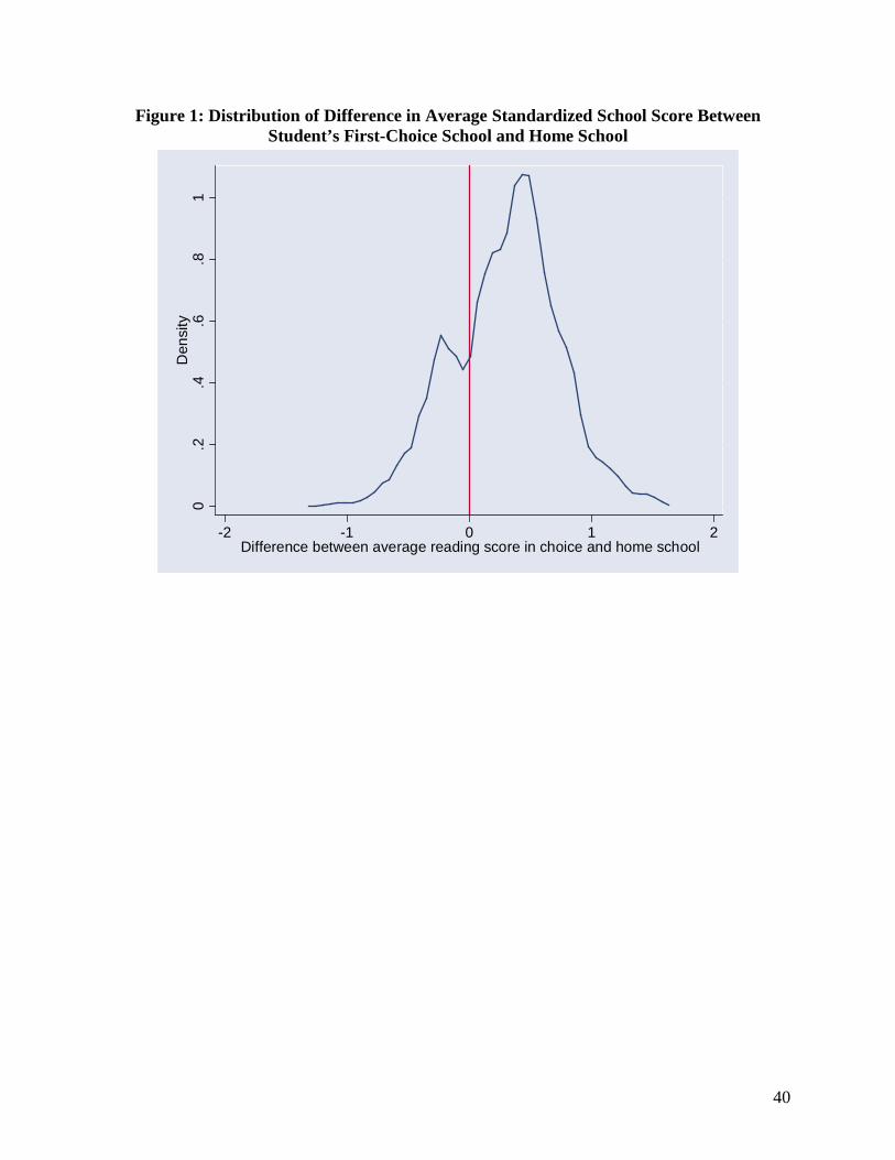
40

Figure 1: Distribution of Difference in Average Standardized School Score Between Student’s First-Choice School and Home School

0.2

.4.6

.81

Den

sity

-2 -1 0 1 2Difference between average reading score in choice and home school

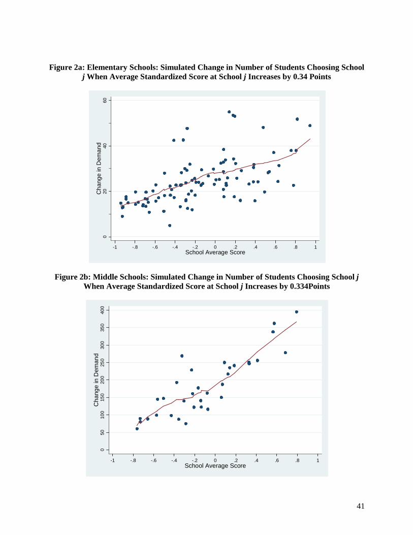
41

Figure 2a: Elementary Schools: Simulated Change in Number of Students Choosing School j When Average Standardized Score at School j Increases by 0.34 Points

Figure 2b: Middle Schools: Simulated Change in Number of Students Choosing School j When Average Standardized Score at School j Increases by 0.334Points

020

4060

Cha

nge

in D

eman

d

-1 -.8 -.6 -.4 -.2 0 .2 .4 .6 .8 1School Average Score

050

100

150

200

250

300

350

400

Cha

nge

in D

eman

d

-1 -.8 -.6 -.4 -.2 0 .2 .4 .6 .8 1School Average Score

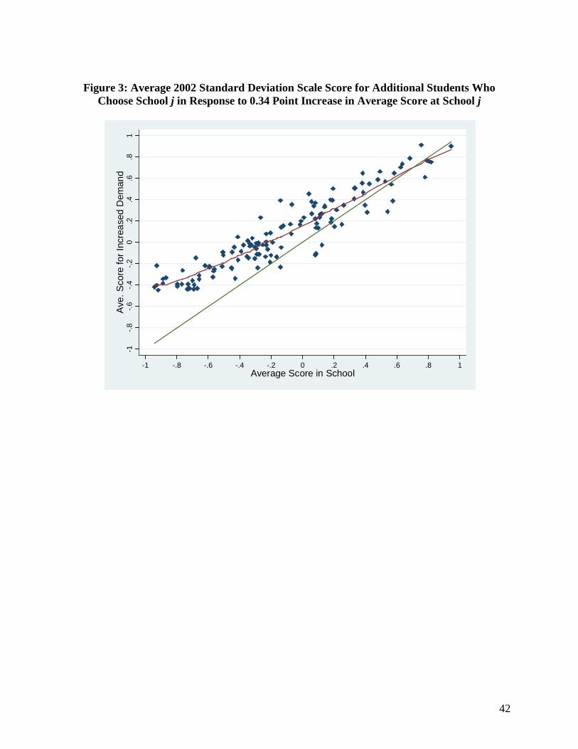
42

Figure 3: Average 2002 Standard Deviation Scale Score for Additional Students Who

Choose School j in Response to 0.34 Point Increase in Average Score at School j

-1-.8

-.6-.4

-.20

.2.4

.6.8

1A

ve. S

core

for I

ncre

ased

Dem

and

-1 -.8 -.6 -.4 -.2 0 .2 .4 .6 .8 1Average Score in School

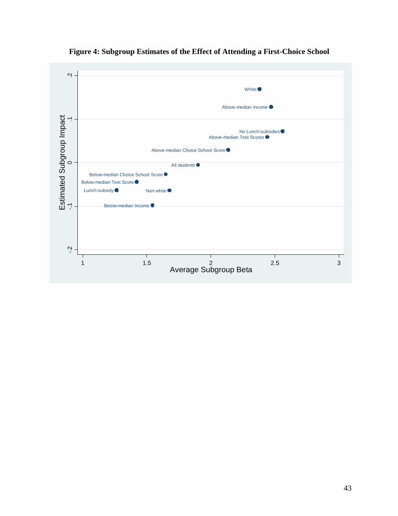
43

Figure 4: Subgroup Estimates of the Effect of Attending a First-Choice School

All students

Non-white

White

Below-median Income

Above-median Income

No Lunch-subsidies

Lunch-subsidy

Below-median Test Score

Above-median Test Scores

Below-median Choice School Score

Above-median Choice School Score

-.2-.1

0.1

.2E

stim

ated

Sub

grou

p Im

pact

1 1.5 2 2.5 3Average Subgroup Beta

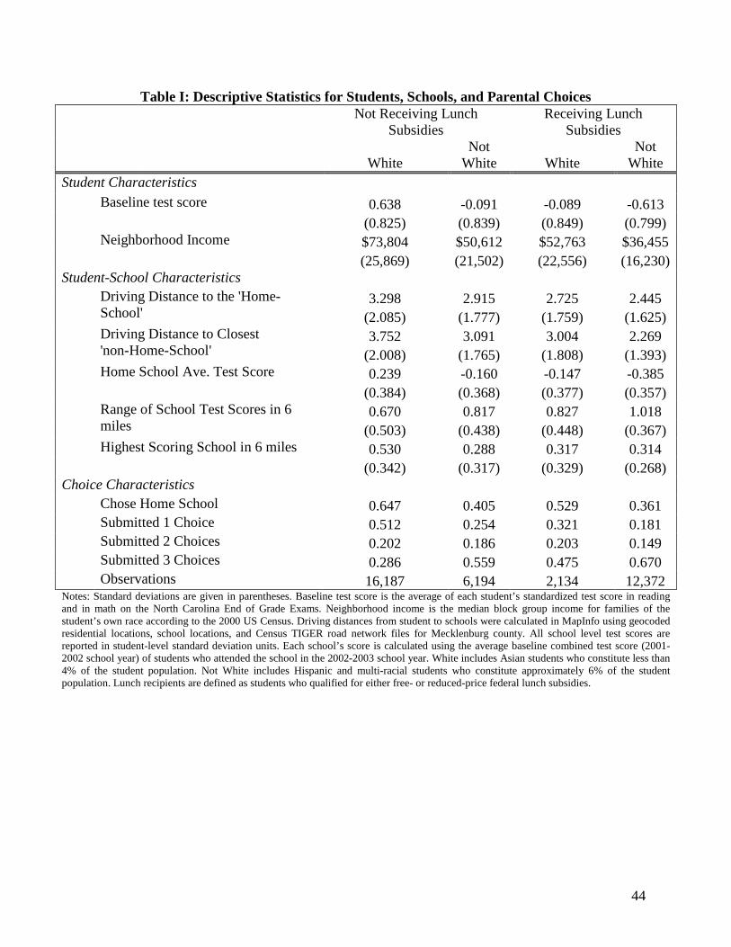
44

Table I: Descriptive Statistics for Students, Schools, and Parental Choices

Not Receiving Lunch

Subsidies Receiving Lunch

Subsidies

White Not

White White Not

White Student Characteristics Baseline test score 0.638 -0.091 -0.089 -0.613 (0.825) (0.839) (0.849) (0.799) Neighborhood Income $73,804 $50,612 $52,763 $36,455 (25,869) (21,502) (22,556) (16,230) Student-School Characteristics Driving Distance to the 'Home-

School' 3.298 2.915 2.725 2.445

(2.085) (1.777) (1.759) (1.625) Driving Distance to Closest

'non-Home-School' 3.752 3.091 3.004 2.269

(2.008) (1.765) (1.808) (1.393) Home School Ave. Test Score 0.239 -0.160 -0.147 -0.385 (0.384) (0.368) (0.377) (0.357) Range of School Test Scores in 6

miles 0.670 0.817 0.827 1.018

(0.503) (0.438) (0.448) (0.367) Highest Scoring School in 6 miles 0.530 0.288 0.317 0.314 (0.342) (0.317) (0.329) (0.268) Choice Characteristics Chose Home School 0.647 0.405 0.529 0.361 Submitted 1 Choice 0.512 0.254 0.321 0.181 Submitted 2 Choices 0.202 0.186 0.203 0.149 Submitted 3 Choices 0.286 0.559 0.475 0.670 Observations 16,187 6,194 2,134 12,372 Notes: Standard deviations are given in parentheses. Baseline test score is the average of each student’s standardized test score in reading and in math on the North Carolina End of Grade Exams. Neighborhood income is the median block group income for families of the student’s own race according to the 2000 US Census. Driving distances from student to schools were calculated in MapInfo using geocoded residential locations, school locations, and Census TIGER road network files for Mecklenburg county. All school level test scores are reported in student-level standard deviation units. Each school’s score is calculated using the average baseline combined test score (2001-2002 school year) of students who attended the school in the 2002-2003 school year. White includes Asian students who constitute less than 4% of the student population. Not White includes Hispanic and multi-racial students who constitute approximately 6% of the student population. Lunch recipients are defined as students who qualified for either free- or reduced-price federal lunch subsidies.

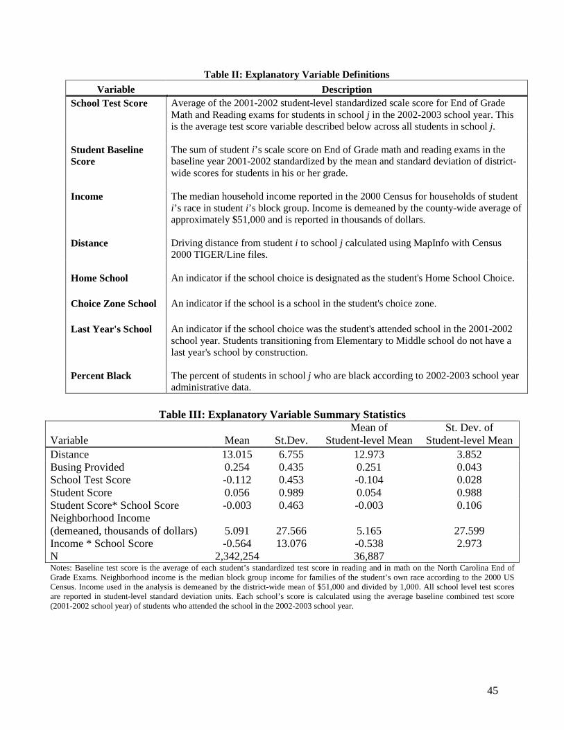
45

Table II: Explanatory Variable Definitions Variable Description

School Test Score Average of the 2001-2002 student-level standardized scale score for End of Grade Math and Reading exams for students in school j in the 2002-2003 school year. This is the average test score variable described below across all students in school j.

Student Baseline Score

The sum of student i’s scale score on End of Grade math and reading exams in the baseline year 2001-2002 standardized by the mean and standard deviation of district-wide scores for students in his or her grade.

Income The median household income reported in the 2000 Census for households of student

i’s race in student i’s block group. Income is demeaned by the county-wide average of approximately $51,000 and is reported in thousands of dollars.

Distance Driving distance from student i to school j calculated using MapInfo with Census

2000 TIGER/Line files. Home School An indicator if the school choice is designated as the student's Home School Choice. Choice Zone School An indicator if the school is a school in the student's choice zone. Last Year's School An indicator if the school choice was the student's attended school in the 2001-2002

school year. Students transitioning from Elementary to Middle school do not have a last year's school by construction.

Percent Black The percent of students in school j who are black according to 2002-2003 school year

administrative data.

Table III: Explanatory Variable Summary Statistics

Variable Mean St.Dev. Mean of

Student-level Mean St. Dev. of

Student-level Mean Distance 13.015 6.755 12.973 3.852 Busing Provided 0.254 0.435 0.251 0.043 School Test Score -0.112 0.453 -0.104 0.028 Student Score 0.056 0.989 0.054 0.988 Student Score* School Score -0.003 0.463 -0.003 0.106 Neighborhood Income (demeaned, thousands of dollars) 5.091 27.566 5.165 27.599 Income * School Score -0.564 13.076 -0.538 2.973 N 2,342,254 36,887 Notes: Baseline test score is the average of each student’s standardized test score in reading and in math on the North Carolina End of Grade Exams. Neighborhood income is the median block group income for families of the student’s own race according to the 2000 US Census. Income used in the analysis is demeaned by the district-wide mean of $51,000 and divided by 1,000. All school level test scores are reported in student-level standard deviation units. Each school’s score is calculated using the average baseline combined test score (2001-2002 school year) of students who attended the school in the 2002-2003 school year.

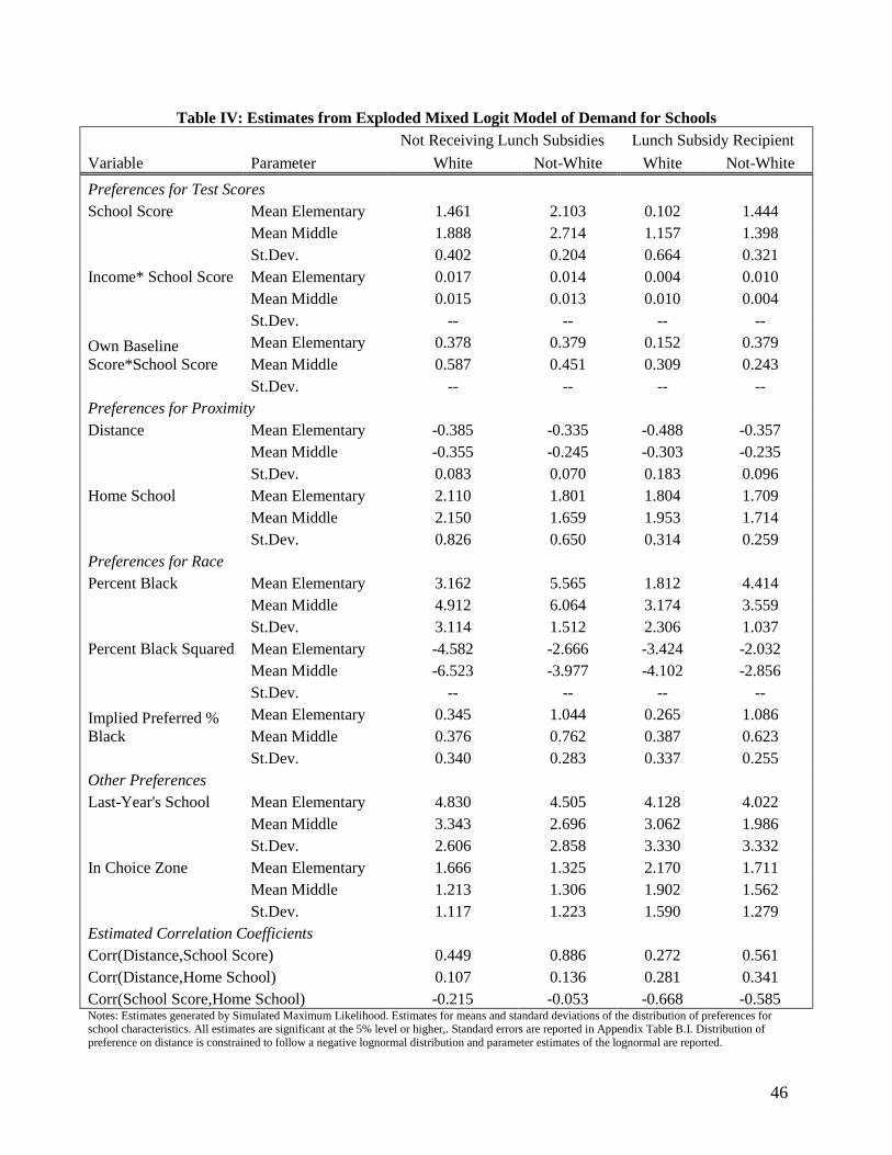
46

Table IV: Estimates from Exploded Mixed Logit Model of Demand for Schools Not Receiving Lunch Subsidies Lunch Subsidy Recipient Variable Parameter White Not-White White Not-White Preferences for Test Scores School Score Mean Elementary 1.461 2.103 0.102 1.444 Mean Middle 1.888 2.714 1.157 1.398 St.Dev. 0.402 0.204 0.664 0.321 Income* School Score Mean Elementary 0.017 0.014 0.004 0.010 Mean Middle 0.015 0.013 0.010 0.004 St.Dev. -- -- -- -- Own Baseline Score*School Score

Mean Elementary 0.378 0.379 0.152 0.379 Mean Middle 0.587 0.451 0.309 0.243

St.Dev. -- -- -- -- Preferences for Proximity Distance Mean Elementary -0.385 -0.335 -0.488 -0.357 Mean Middle -0.355 -0.245 -0.303 -0.235 St.Dev. 0.083 0.070 0.183 0.096 Home School Mean Elementary 2.110 1.801 1.804 1.709 Mean Middle 2.150 1.659 1.953 1.714 St.Dev. 0.826 0.650 0.314 0.259 Preferences for Race Percent Black Mean Elementary 3.162 5.565 1.812 4.414 Mean Middle 4.912 6.064 3.174 3.559 St.Dev. 3.114 1.512 2.306 1.037 Percent Black Squared Mean Elementary -4.582 -2.666 -3.424 -2.032 Mean Middle -6.523 -3.977 -4.102 -2.856 St.Dev. -- -- -- -- Implied Preferred % Black

Mean Elementary 0.345 1.044 0.265 1.086 Mean Middle 0.376 0.762 0.387 0.623

St.Dev. 0.340 0.283 0.337 0.255 Other Preferences Last-Year's School Mean Elementary 4.830 4.505 4.128 4.022 Mean Middle 3.343 2.696 3.062 1.986 St.Dev. 2.606 2.858 3.330 3.332 In Choice Zone Mean Elementary 1.666 1.325 2.170 1.711 Mean Middle 1.213 1.306 1.902 1.562 St.Dev. 1.117 1.223 1.590 1.279 Estimated Correlation Coefficients Corr(Distance,School Score) 0.449 0.886 0.272 0.561 Corr(Distance,Home School) 0.107 0.136 0.281 0.341 Corr(School Score,Home School) -0.215 -0.053 -0.668 -0.585 Notes: Estimates generated by Simulated Maximum Likelihood. Estimates for means and standard deviations of the distribution of preferences for school characteristics. All estimates are significant at the 5% level or higher,. Standard errors are reported in Appendix Table B.I. Distribution of preference on distance is constrained to follow a negative lognormal distribution and parameter estimates of the lognormal are reported.

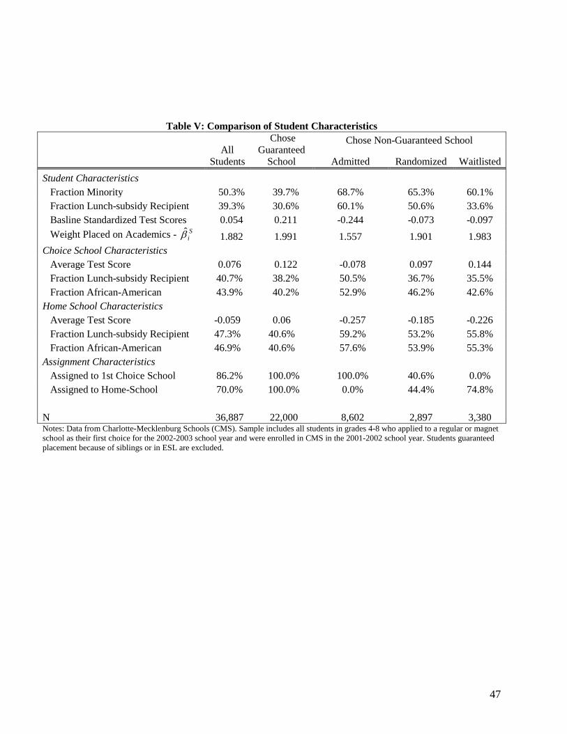
47

Table V: Comparison of Student Characteristics

All

Students

Chose Guaranteed

School

Chose Non-Guaranteed School

Admitted Randomized Waitlisted Student Characteristics

Fraction Minority 50.3% 39.7% 68.7% 65.3% 60.1% Fraction Lunch-subsidy Recipient 39.3% 30.6% 60.1% 50.6% 33.6% Basline Standardized Test Scores 0.054 0.211 -0.244 -0.073 -0.097 Weight Placed on Academics - S

iβ̂ 1.882 1.991 1.557 1.901 1.983 Choice School Characteristics

Average Test Score 0.076 0.122 -0.078 0.097 0.144 Fraction Lunch-subsidy Recipient 40.7% 38.2% 50.5% 36.7% 35.5% Fraction African-American 43.9% 40.2% 52.9% 46.2% 42.6% Home School Characteristics

Average Test Score -0.059 0.06 -0.257 -0.185 -0.226 Fraction Lunch-subsidy Recipient 47.3% 40.6% 59.2% 53.2% 55.8% Fraction African-American 46.9% 40.6% 57.6% 53.9% 55.3% Assignment Characteristics

Assigned to 1st Choice School 86.2% 100.0% 100.0% 40.6% 0.0% Assigned to Home-School 70.0% 100.0% 0.0% 44.4% 74.8%

N 36,887 22,000 8,602 2,897 3,380 Notes: Data from Charlotte-Mecklenburg Schools (CMS). Sample includes all students in grades 4-8 who applied to a regular or magnet school as their first choice for the 2002-2003 school year and were enrolled in CMS in the 2001-2002 school year. Students guaranteed placement because of siblings or in ESL are excluded.

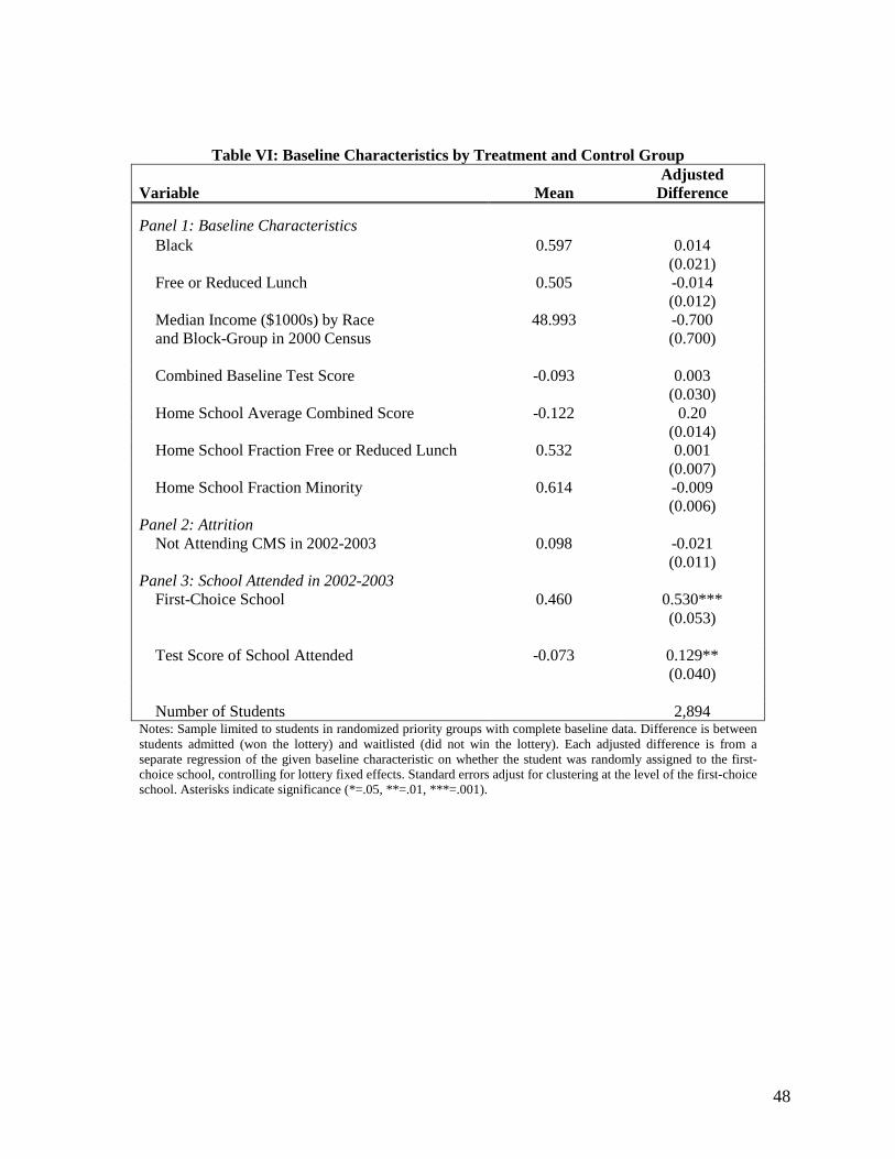
48

Table VI: Baseline Characteristics by Treatment and Control Group

Variable Mean Adjusted

Difference

Panel 1: Baseline Characteristics Black 0.597 0.014 (0.021) Free or Reduced Lunch 0.505 -0.014 (0.012) Median Income ($1000s) by Race 48.993 -0.700 and Block-Group in 2000 Census (0.700)

Combined Baseline Test Score -0.093 0.003 (0.030) Home School Average Combined Score -0.122 0.20 (0.014) Home School Fraction Free or Reduced Lunch 0.532 0.001 (0.007) Home School Fraction Minority 0.614 -0.009 (0.006)

Panel 2: Attrition Not Attending CMS in 2002-2003 0.098 -0.021 (0.011)

Panel 3: School Attended in 2002-2003 First-Choice School 0.460 0.530*** (0.053) Test Score of School Attended -0.073 0.129** (0.040) Number of Students 2,894

Notes: Sample limited to students in randomized priority groups with complete baseline data. Difference is between students admitted (won the lottery) and waitlisted (did not win the lottery). Each adjusted difference is from a separate regression of the given baseline characteristic on whether the student was randomly assigned to the first-choice school, controlling for lottery fixed effects. Standard errors adjust for clustering at the level of the first-choice school. Asterisks indicate significance (*=.05, **=.01, ***=.001).

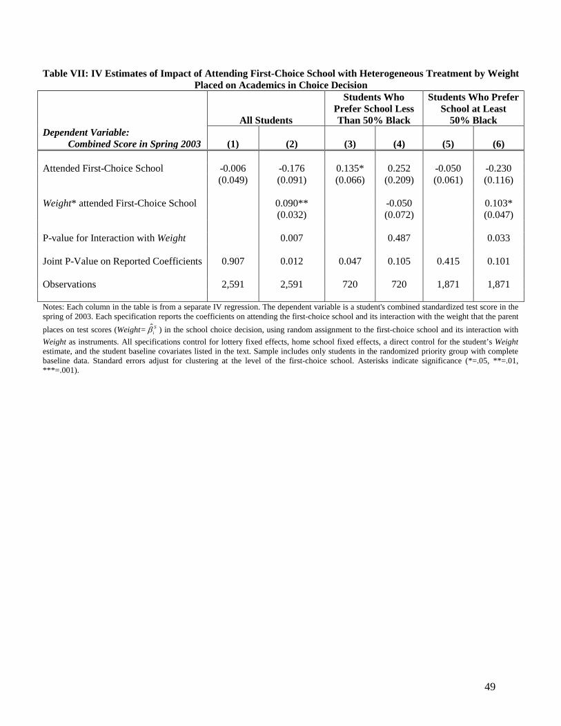
49

Table VII: IV Estimates of Impact of Attending First-Choice School with Heterogeneous Treatment by Weight Placed on Academics in Choice Decision

Dependent Variable: Combined Score in Spring 2003

All Students

Students Who Prefer School Less Than 50% Black

Students Who Prefer School at Least

50% Black

(1) (2)

(3)

(4)

(5)

(6) Attended First-Choice School -0.006 -0.176 0.135* 0.252 -0.050 -0.230 (0.049) (0.091) (0.066) (0.209) (0.061) (0.116) Weight* attended First-Choice School 0.090** -0.050 0.103* (0.032) (0.072) (0.047) P-value for Interaction with Weight 0.007 0.487 0.033 Joint P-Value on Reported Coefficients 0.907 0.012 0.047 0.105 0.415 0.101 Observations 2,591 2,591 720 720 1,871 1,871 Notes: Each column in the table is from a separate IV regression. The dependent variable is a student's combined standardized test score in the spring of 2003. Each specification reports the coefficients on attending the first-choice school and its interaction with the weight that the parent places on test scores (Weight= S

iβ̂ ) in the school choice decision, using random assignment to the first-choice school and its interaction with Weight as instruments. All specifications control for lottery fixed effects, home school fixed effects, a direct control for the student’s Weight estimate, and the student baseline covariates listed in the text. Sample includes only students in the randomized priority group with complete baseline data. Standard errors adjust for clustering at the level of the first-choice school. Asterisks indicate significance (*=.05, **=.01, ***=.001).

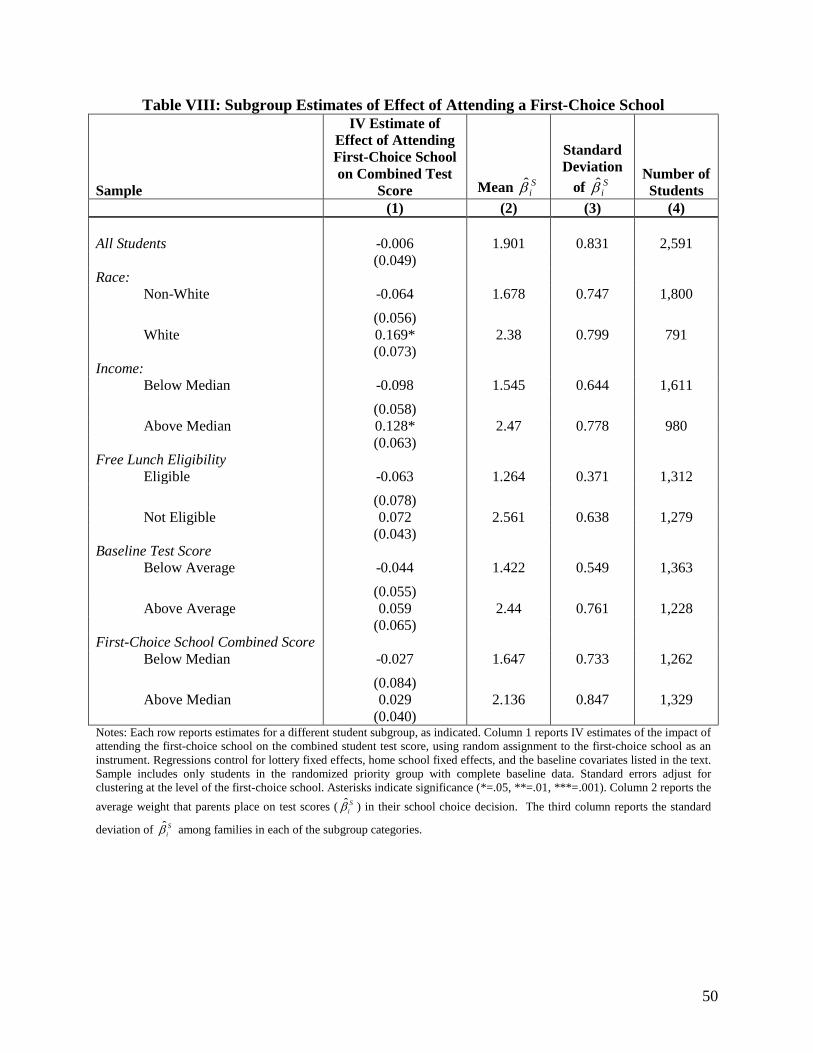
50

Table VIII: Subgroup Estimates of Effect of Attending a First-Choice School

Sample

IV Estimate of Effect of Attending First-Choice School on Combined Test

Score Mean Siβ̂

Standard Deviation

of Siβ̂

Number of Students

(1) (2) (3) (4) All Students -0.006 1.901 0.831 2,591 (0.049) Race: Non-White -0.064 1.678 0.747 1,800 (0.056) White 0.169* 2.38 0.799 791 (0.073) Income: Below Median -0.098 1.545 0.644 1,611 (0.058) Above Median 0.128* 2.47 0.778 980 (0.063) Free Lunch Eligibility Eligible -0.063 1.264 0.371 1,312 (0.078) Not Eligible 0.072 2.561 0.638 1,279 (0.043) Baseline Test Score Below Average -0.044 1.422 0.549 1,363 (0.055) Above Average 0.059 2.44 0.761 1,228 (0.065) First-Choice School Combined Score Below Median -0.027 1.647 0.733 1,262 (0.084) Above Median 0.029 2.136 0.847 1,329 (0.040) Notes: Each row reports estimates for a different student subgroup, as indicated. Column 1 reports IV estimates of the impact of attending the first-choice school on the combined student test score, using random assignment to the first-choice school as an instrument. Regressions control for lottery fixed effects, home school fixed effects, and the baseline covariates listed in the text. Sample includes only students in the randomized priority group with complete baseline data. Standard errors adjust for clustering at the level of the first-choice school. Asterisks indicate significance (*=.05, **=.01, ***=.001). Column 2 reports the average weight that parents place on test scores ( S

iβ̂ ) in their school choice decision. The third column reports the standard

deviation of Siβ̂ among families in each of the subgroup categories.