DI

SC

US

SI

ON

P

AP

ER

S

ER

IE

S

Forschungsinstitut zur Zukunft der ArbeitInstitute for the Study of Labor

Welfare, Labor Supply and Heterogeneous Preferences:Evidence for Europe and the US

IZA DP No. 6102

November 2011

Olivier BargainAndré DecosterMathias Dolls

Dirk NeumannAndreas PeichlSebastian Siegloch

Welfare, Labor Supply and Heterogeneous Preferences:

Evidence for Europe and the US

Olivier Bargain Aix-Marseille School of Economics,

IZA and CEPS/INSTEAD

André Decoster CES, KU Leuven

Mathias Dolls

IZA and University of Cologne

Dirk Neumann IZA and University of Cologne

Andreas Peichl

IZA, University of Cologne, ISER and CESifo

Sebastian Siegloch IZA and University of Cologne

Discussion Paper No. 6102

November 2011 (updated: September 2012)

IZA

P.O. Box 7240 53072 Bonn

Germany

Phone: +49-228-3894-0 Fax: +49-228-3894-180

E-mail: iza@iza.org

Any opinions expressed here are those of the author(s) and not those of IZA. Research published in this series may include views on policy, but the institute itself takes no institutional policy positions. The Institute for the Study of Labor (IZA) in Bonn is a local and virtual international research center and a place of communication between science, politics and business. IZA is an independent nonprofit organization supported by Deutsche Post Foundation. The center is associated with the University of Bonn and offers a stimulating research environment through its international network, workshops and conferences, data service, project support, research visits and doctoral program. IZA engages in (i) original and internationally competitive research in all fields of labor economics, (ii) development of policy concepts, and (iii) dissemination of research results and concepts to the interested public. IZA Discussion Papers often represent preliminary work and are circulated to encourage discussion. Citation of such a paper should account for its provisional character. A revised version may be available directly from the author.

IZA Discussion Paper No. 6102 November 2011 (updated: September 2012)

ABSTRACT

Welfare, Labor Supply and Heterogeneous Preferences: Evidence for Europe and the US*

Following the report of the Stiglitz Commission, measuring and comparing well-being across countries has gained renewed interest. Yet, analyses that go beyond income and incorporate non-market dimensions of welfare most often rely on the assumption of identical preferences to avoid the difficulties related to interpersonal comparisons. In this paper, we suggest an international comparison based on individual welfare rankings that fully retain preference heterogeneity. Focusing on the consumption-leisure trade-off, we estimate discrete choice labor supply models using harmonized microdata for 11 European countries and the US. We retrieve preference heterogeneity within and across countries and analyze several welfare criteria which take into account that differences in income are partly due to differences in tastes. The resulting welfare rankings clearly depend on the normative treatment of preference heterogeneity with alternative metrics. We show that these differences can indeed be explained by estimated preference heterogeneity across countries – rather than demographic composition. JEL Classification: C35, D63, H24, H31, J22 Keywords: welfare measures, preference heterogeneity, labor supply, Beyond GDP Corresponding author: Dirk Neumann IZA P.O. Box 7240 53072 Bonn Germany E-mail: dneumann@iza.org

* This paper uses TAXSIM version v9 which is based on the IPUMS CPS, an integrated set of data of the March Current Population Survey which is conducted jointly by the U.S. Census Bureau and the Bureau of Labor Statistics. Furthermore we use EUROMOD version D16. Here, the ECHP and EU-SILC were made available by Eurostat; the Austrian version of the ECHP by Statistik Austria; the PSBH by the University of Liège and the University of Antwerp; the IDS by Statistics Finland; the EBF by INSEE; the GSOEP by DIW Berlin; the Living in Ireland Survey by the ESRI; the SEP by Statistics Netherlands; the IDS by Statistics Sweden; and the FES by the UK ONS through the Data Archive. Material from the FES is Crown Copyright and is used by permission. None of the institutions cited above bear any responsibility for the analysis or interpretation of the data reported here. Andreas Peichl is grateful for financial support by Deutsche Forschungsgemeinschaft DFG (PE1675). We would like to thank Bart Capéau, Koen Decancq, Erwin Ooghe, Andrew Oswald, two anonymous referees, the editor Marc Fleurbaey, as well as seminar and conference participants in Ann Arbor (IIPF), Bonn (IZA), Canazei (IT), Chicago (SOLE), Dublin (ISNE), Essex (ISER), Leuven (CES), Paris (New Directions in Welfare, OECD) and Stockholm (IMA) for useful comments and suggestions. We are indebted to all past and current members of the EUROMOD consortium for the construction and development of EUROMOD and to Daniel Feenberg and the NBER for granting us access to TAXSIM. The usual disclaimer applies.

1 Introduction

Following the report of the Stiglitz commission (Stiglitz et al, 2009), there has been a

recurrent interest in measuring and comparing well-being within and especially across

countries (e.g. Jones and Klenow, 2010). One main motivation of the report was to move

‘beyond GDP’ by recognizing the multi-dimensional character of welfare. In addition, re-

cent contributions in the theory of social choice and fair allocation shed new light on how

to reasonably measure and consistently compare individual well-being once certain non-

market domains are considered besides income and given that individuals have different

preferences over the various dimensions of life (see e.g. Fleurbaey, 2011). In the economic

literature, one of the basic sources of well-being besides income is leisure time, resulting

in the consumption-leisure trade-off in labor supply modeling. However, while there has

been substantial progress in the development of positive labor supply models in terms

of (structurally) estimating individual consumption-leisure preferences, the heterogeneity

in preferences is usually neglected in the normative part of the analysis concerned with

welfare evaluation. This is due to the difficulties related to interpersonal welfare compar-

isons. A prominent approach to solve this issue is to use preferences of a certain reference

household (e.g. Aaberge et al, 2004; Aaberge and Colombino, 2011). Clearly, this makes

individual well-being comparable but the heterogeneity in preferences is assumed away. In

this paper, we contrast this approach to welfare measures that fully account for different

individual consumption-leisure preferences (Fleurbaey, 2006, 2008) and suggest an inter-

national comparison based on pure orderings of individual well-being. Then, we illustrate

that the choice of how to treat heterogeneity in preferences may substantially affect the

evaluation of welfare across different countries.

The empirical application starts with the estimation of labor supply models, separately

for 11 European countries1 and the US. Focusing on married women, the group most

studied in the literature, we rely on 12 representative micro-datasets (on household net

income, hours worked and various socio-demographics) and a harmonized econometric

approach for all countries in order to obtain comparable estimates of consumption-leisure

preferences. We make use of a common structural discrete choice model for labor supply,

as used in well-known contributions for Europe (e.g. Van Soest, 1995) or the US (e.g.

Eissa and Hoynes, 2004). This allows us to account for the comprehensive and usually

non-linear effect of tax-benefit systems on household budgets, which contributes to the

identification of the preference parameters. As the labor supply model is identified via a

direct parametrization of the utility function, we are then able to obtain indifference curves

for all individuals of all countries - and take only this ordinal information on well-being to

1These are Austria (AT), Belgium (BE), Denmark (DK), Finland (FI), France (FR), Germany (GE),Ireland (IE), the Netherlands (NL), Portugal (PT), Sweden (SW) and the United Kingdom (UK).

1

derive an international ranking of individual situations for each of the alternative welfare

metrics. These rankings are simple index orderings reflecting interpersonal comparisons

of individual utilities and are not based on any kind of a social aggregator function.

The main results go as follows. First, we contrast the standard approaches of using

pure income or classic money metric utilities based on a reference household to that of

taking preference heterogeneity into account. Second, once heterogeneity in tastes is ac-

counted for, our findings suggest that the resulting ranking of individuals across countries

remarkably depends on the normative choice related to the metric at use. Precisely, with

a metric that evaluates agents with a higher willingness-to-work to be better off compared

to agents with a lower willingness-to-work, households from countries where average fe-

male working hours are rather high (as in the US and the Nordic countries) perform better

on average compared to a ranking based on income only. Inversely, for countries where

average working hours are rather low (as in most Continental European countries, Ireland

and the UK), the same holds true with a metric that considers agents with a relatively

lower willingness-to-work as better off. This leads to substantial reranking across nations

when moving from the former to the latter type of criteria – with remarkable changes

in average individual percentile positions of at least 15 percentage points for 7 out of

12 countries. Third, we decompose marginal rates of substitution (MRS) to extract the

role of different sources of heterogeneity for this result. We find that different rankings

across welfare metrics are mainly due to heterogeneous work preferences across countries

– rather than demographic composition. Thus, the analysis clearly shows that respecting

preference heterogeneity may have substantial influences when comparing well-being in

an international context. We believe that these concerns should precede any attempts

to compare countries on the basis of social welfare functions (SWF) or other forms of

aggregated indices.

The rest of the paper is structured as follows. Section 2 gives an overview of the related

literature. In Section 3 we review the welfare criteria and their normative interpretation.

Section 4 describes the empirical implementation, including the labor supply model, the

data and descriptive information. In Section 5 we present and discuss the main results

together with some robustness checks. Section 6 concludes.

2 Related literature

Related to the present paper, several studies have recently attempted to provide inter-

national comparisons of welfare levels relying on an equivalent income approach when

2

accounting for non-material aspects of well-being.2 Becker et al (2005) correct growth

rates for life expectancy (as an indicator for quality of life). Fleurbaey and Gaulier (2009)

consider leisure, risk of unemployment, health and household composition besides GDP

in OECD countries. For a large set of 134 countries over time, Jones and Klenow (2010)

focus on consumption rather than income when accounting for several other dimensions of

well-being. Importantly, all these studies have in common that they compute equivalent

incomes at the country level assuming identical preferences across individuals (i.e., relying

on a representative agent approach). Aggregation and comparison across countries follows

by use of a SWF. However, as already pointed out by Fleurbaey and Gaulier (2009, p.

620), for “an accurate application of this methodology, one needs survey data on income

and on the additional dimensions of consumption [...], as well as on preferences [...], at

the individual level and for all the countries studied.” This is precisely the path we take

in the present paper.

As standard in the labor supply literature, we retrieve individual and cross-country

specific preference heterogeneity relying on a structural discrete choice model. Naturally,

such models respect individual differences in the taste for consumption versus leisure

when estimating preference parameters. However, when it comes to welfare analyses, we

typically observe that preference heterogeneity is neglected. The main reason is the well-

known trade-off between ensuring interpersonal comparability and respecting individual

preferences (see e.g. Fleurbaey and Trannoy, 2003; Brun and Tungodden, 2004).3 In em-

pirical labor supply modeling, two main approaches emerged (besides the simple – but

still prominent – use of income as a welfare index). One is to mention, but de facto neglect

the comparability and aggregation problems in presence of preference heterogeneity and

to report averages of individual – uncomparable – equivalent or compensating variations

(see e.g. Aaberge et al, 1995, 2000; Dagsvik et al, 2009) or to aggregate them using a

certain SWF (e.g. Eissa et al, 2008; Fuest et al, 2008; Creedy and Herault, 2012).4 In

contrast, a second approach explicitly addresses the comparability issue using a reference

household for welfare analyses. Following King (1983), classic individual money-metric

utilities are derived by means of a fixed preference function at fixed reference prices (e.g.

Aaberge et al, 2004; Ericson and Flood, 2009; Aaberge and Colombino, 2011). However,

with this approach, preferences of a certain reference household build the basis for com-

2For a comprehensive overview on general attempts to construct measures of social welfare alternativeto GDP, see Fleurbaey (2009). Kassenboehmer and Schmidt (2011) critically assess the additional valueof taking into account alternative components to GDP.

3A related, more practical reason might be that even if differences in individual preferences wereaccounted for, it could become a very complicated normative exercise to determine the weights assignedto individual utilities in order to aggregate them.

4Indeed, reference prices (wages) for calculations of equivalent and compensating variations are nat-urally individual and thus, variable. Aggregated indices based on equivalent or compensating variationsare therefore inconsistent as long as they are not based on a representative agent approach.

3

paring individual well-being, which are hence no longer individual specific but unified and

determined by the social planner.5

In the present paper we adopt an approach from the recent social choice literature that

allows to fully respect individual preferences in welfare analyses (Fleurbaey, 2006, 2008,

2011; Fleurbaey and Maniquet, 2006). In this approach, interpersonal comparisons can be

conceived directly in terms of subsets of the consumption-leisure space which are nested

into each other. The chosen bundle on a given indifference curve can thus be evaluated

based on the subset that is tangent to the individual indifference curve. This allows

deriving a welfare metric which will be clearly ordered for different preferences, making

individual situations unambiguously comparable. In the consumption-leisure context, the

derivation of comparable, nested subsets requires to either fix a specific net wage rate

or a certain amount of non-labor income. While this procedure is thus similar to the

derivation of classic equivalent incomes, the choice of the reference values is grounded

on specific fairness considerations. This makes the normative priors of the interpersonal

comparison more explicit – as, e.g., requested by Atkinson (2011).6 So far, measures of

this kind have not been implemented empirically except in Decoster and Haan (2010)

and the present paper. While those authors address preference heterogeneity within a

country (Germany), we compute equivalent incomes for individuals of 12 countries and

analyze how international rankings vary with the use of alternative welfare metrics. In

particular, we focus on the extent to which welfare evaluation is affected by that part

of heterogeneous work preferences which is genuinely country-specific.7 In addition, we

assess the role of different sources of heterogeneity for the resulting differences in welfare

rankings.

5Then, welfare changes are usually evaluated using a certain SWF over individual money-metricutilities. This generated another stream of criticism, initiated by Blackorby and Donaldson (1988): aSWF over equivalent incomes usually fails to be quasi-concave in commodity consumptions which isincompatible with a minimal preference for equality.

6Choosing reference values based on certain fairness considerations is the actual novelty of the fairallocation approach compared to classical demand theory when deriving equivalent incomes. See Prestonand Walker (1999), for instance, who derive a similar set of metrics in line with the latter. More popular,however, has been the alternative of exploring reference price independent comparisons of individualwelfare (see e.g. Roberts, 1980; Slesnick, 1991; Blackorby et al, 1993).

7This can also be motivated by a prominent debate about what determines differences in labor supplybehavior across countries, particularly between Europe and the US. Prescott (2004) states that differentlabor supply elasticities are almost only due to differences in tax-transfer systems. This view has beencriticized by Blanchard (2004) who – in line with Alesina et al (2005) – argues that different preferencesfor leisure indeed play a role and are maybe due to cultural differences. Our findings, which control forcountry-specific consumption-leisure preferences, tend to support the latter view.

4

3 Theoretical framework

In order to respect preference heterogeneity in the consumption-leisure space, we follow

Fleurbaey (2006, 2008) and look at individual welfare measures which specifically differ in

the way they treat heterogeneity in tastes. In the following, we introduce these measures

and their underlying normative rationales. We refer to Fleurbaey (2006, 2008) for the

axiomatic derivation and to Decoster and Haan (2010) for a more detailed illustration.

However, while those studies define the metrics in the usual social choice terminology

(i.e. as means of budget sets), we “translate” them into the language of classical demand

theory in order to bring them closer to the usual notation used for welfare analyses in

(empirical) labor supply models.

The setup. Assume that agent i has individual preferences over consumption ci and

labor time hi, denoted Ri, and ci ∈ R+, hi ∈ [0, 1]. By Ri, agent i weakly prefers

bundle (ci, hi) over bundle (c′i, h

′i), with use of a preference representation function ui

leading to (ci, hi)Ri(c′i, h

′i) ⇔ ui(ci, hi) ≥ ui(c

′i, h

′i). Observed preference heterogeneity is

introduced via an individual specific vector zi (containing all characteristics determin-

ing individual preferences), Ri = R(zi), and thus ui(ci, hi) = u(ci, hi; zi). The chosen

bundle (ci, hi) results from a classic individual utility maximization problem. Let f(.)

represent the tax-transfer function that transforms gross non-labor income Ii and gross

labor income wih (with wi denoting individual i’s gross wage) into net income c, i.e.

(ci, hi) = max [u(c, h; zi)|c ≤ f(Ii, wih), h ≤ 1]. Hence, the observed bundle of consump-

tion and leisure results from individual choices subject to preferences and a budget con-

straint.

The welfare metrics. Assume the individual’s utility function u(ci, hi; zi) = ui(ci, hi)

to be well-behaved, i.e. continuous and increasing in their arguments as well as quasicon-

cave in (c, h). Furthermore, assume tax-transfer rules f(.) determining individual budget

sets c ≤ f(Ii, wih) to be non-linear – as generally observed in reality. Then, for each chosen

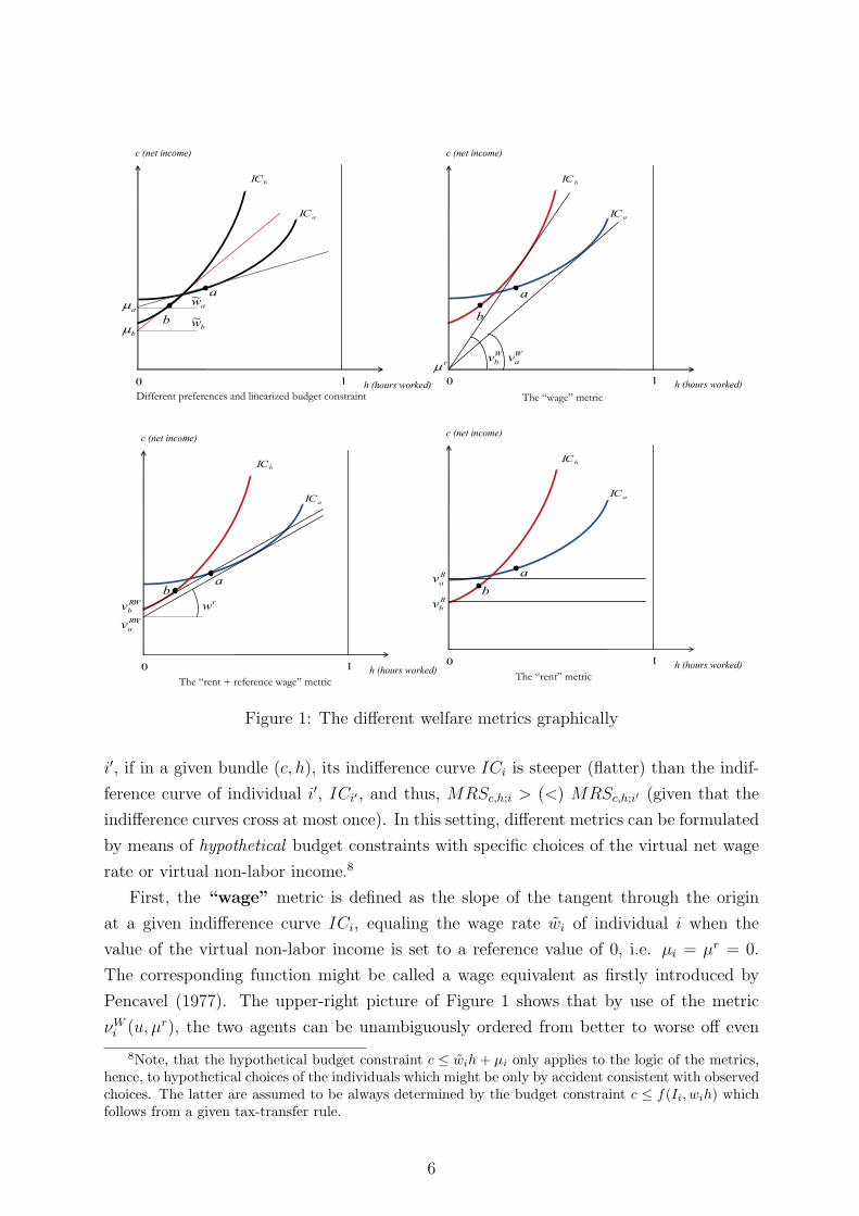
bundle (ci, hi) on a given individual indifference curve ICi = ci(u, hi) = min[ci|ui(ci, hi) ≥u], an associated hypothetical, linear budget constraint that would leave the individual

indifferent between choosing from this or her actual budget, can be derived as c ≤ wih+µi

with virtual non-labor income µi determined by virtual net wage wi - as illustrated for

bundles a and b in the upper-left panel of Figure 1. For the definition of different metrics

below we further define the expenditure function ei(u, wi) = min[ci − wihi|ui(ci, hi) ≥ u],

with a fixed level of utility u. The slope of the indifference curve in a given bundle (c, h)

is defined as the MRS between consumption and hours worked, MRSc,h = −∂u/∂h∂u/∂c

. An

individual i is characterized to be relatively more (less) work averse than an individual

5

bw~

aw~

c (net income)

h (hours worked)

b

a

Different preferences and linearized budget constraint

0

aIC

bIC

aµ

bµ

1

c (net income)

h (hours worked)

a

b

bIC

aIC

W

bv W

av

The “wage” metric

0

rµ

1

ab

c (net income)

h (hours worked)

RW

av

RW

bvrw

0

aIC

bIC

The “rent + reference wage” metric

1 h (hours worked)

c (net income)

b

aR

av

R

bv

0

aIC

bIC

The “rent” metric

1

Figure 1: The different welfare metrics graphically

i′, if in a given bundle (c, h), its indifference curve ICi is steeper (flatter) than the indif-

ference curve of individual i′, ICi′ , and thus, MRSc,h;i > (<) MRSc,h;i′ (given that the

indifference curves cross at most once). In this setting, different metrics can be formulated

by means of hypothetical budget constraints with specific choices of the virtual net wage

rate or virtual non-labor income.8

First, the “wage” metric is defined as the slope of the tangent through the origin

at a given indifference curve ICi, equaling the wage rate wi of individual i when the

value of the virtual non-labor income is set to a reference value of 0, i.e. µi = µr = 0.

The corresponding function might be called a wage equivalent as firstly introduced by

Pencavel (1977). The upper-right picture of Figure 1 shows that by use of the metric

νWi (u, µr), the two agents can be unambiguously ordered from better to worse off even

8Note, that the hypothetical budget constraint c ≤ wih+ µi only applies to the logic of the metrics,hence, to hypothetical choices of the individuals which might be only by accident consistent with observedchoices. The latter are assumed to be always determined by the budget constraint c ≤ f(Ii, wih) whichfollows from a given tax-transfer rule.

6

though preferences differ:

νWi (u, µr = 0) = min

wi

[wi|vi(wi, µr = 0) ≥ u] (1)

Second, the “rent + reference wage” criterion compares individual situations de-

pending on a certain reference value for the virtual net wage rate, wi = wr. Then, the

resulting welfare metric νRWi (u,wr) is the value of the corresponding virtual non-labor

income given through the expenditure function (bottom-left panel of Figure 1):

νRWi (u,wr) = ei(u,w

r) = minµi

[ci − wrhi|ui(ci, hi) ≥ u] (2)

Third, the “rent” metric directly emerges by setting wi = wr = 0. As far as we

assume well-behaved utility functions, this is equivalent to hours worked being set to a

reference value of hi = hr = 0. The resulting metric νRi (u, h

r) hence is the value of the

intersection of the indifference curve with the ordinate, equaling the corresponding virtual

non-labor income (bottom-right panel of Figure 1):

νRi (u, h

r = 0) = ci(u, 0) = minci

[ci|ui(ci, 0) ≥ u] (3)

Normative interpretation. The key feature of the metrics defined is that they fully

respect preferences: all metrics will increase when the individual moves to a bundle on a

higher indifference curve of her own preference ordering. However, allowing for preference

heterogeneity creates serious problems for interpersonal comparisons of well-being. It

especially raises a question of fairness, i.e., who is to be considered better and worse off

and thus, who should eventually redistribute towards whom - when accounting for the

fact that individual outcomes result not only from endowed circumstances, but also from

individual preferences. The literature on responsibility-sensitive egalitarianism addresses

this problem by keeping individuals responsible for the latter, but not for the former

(Fleurbaey, 2008).

In order to operationalize this principle for social evaluation, two competing inter-

pretations evolved in the economic literature, namely the compensation and the (liberal)

reward principle. The former says that inequalities due to endowed circumstances (i.e.

not due to responsibility factors) should be equalized. In contrast, the latter states that

no further redistribution should be performed beyond what is required by the compensa-

tion principle, remaining neutral towards inequalities due to individual preferences. Even

if similar at a first glance, both principles are logically independent and to some extent

are even in conflict with each other. Note that the three measures defined give priority

to the compensation principle: individuals with poorer hypothetical circumstances are

always ranked worse off and should be compensated (as can be seen from Figure 1). As

7

long as preferences are equal, the metrics will rank individuals in exactly the same way.

However, once preferences differ (as shown in Figure 1 with crossing indifference curves),

on certain occasions, compensation will also depend on the willingness-to-work each agent

reveals. This might lead to favoring the industrious (or work averse) of two individuals in

the given context even if the actual influence of circumstances on outcomes was equal - a

clear conflict with the reward principle. Loosely speaking, the reason is that the influence

of circumstances on outcomes can not be separated from the influence of preferences on

the same outcomes, leading to a clash between the compensation and the reward principle.

In this paper, we are especially interested in the differences between individual welfare

metrics that result from this clash. That is, we study if and how respecting preference

heterogeneity systematically alters interpersonal comparisons of well-being - in an inter-

national empirical context. Thereby, we focus on simple index orderings of individual

well-being levels and do not consider any specific social ordering function. The latter

would go beyond the question of “who is better and worse off” and additionally requires

weighting individual utilities. We restrict ourselves to the former and will thus not perform

any optimization exercise nor do we treat actual redistributive issues between individuals

and/or countries (for this distinction see also Fleurbaey, 2007).

In sum, what is relevant for interpersonal welfare comparisons is the fact that all

the measures defined rank individuals with the same preferences in the same way (i.e.

in accordance with how these individuals would themselves rank their bundles) - while

their sole difference is in the way they treat heterogeneity in tastes. Then, once we accept

that those metrics might remain non-neutral with respect to individual preferences, the

ethical choice at hand is not related to the compensation versus the reward principle but

to the choice of the references for interpersonal comparisons that generate the differences

between the metrics. This is explained in the following.

In a consumption-leisure space, individuals have different preferences for work (result-

ing in different levels of exhibited effort) while skill levels (as reflected in gross wages)

and non-labor income are assumed to be exogenous endowments to the individuals. The

welfare measures defined evaluate individual situations according to hypothetical refer-

ence amounts of those endowments such that they would allow individuals to reach their

current utility level.

First, the “rent” metric asks for the amount of (hypothetical) net income which would

be enough to remain equally well off compared to the initial situation if one did no longer

have to earn it. The resulting metric is simply the level of consumption when working

zero hours which corresponds to the level of virtual non-labor income at a reference wage

of zero. The bottom-right picture of Figure 1 illustrates, that in this case, we judge the

agent who gets bundle b, say Bob, with a relatively lower willingness-to-work to be worse

off compared to the agent who has bundle a, and a higher willingness-to-work, say Ann.

8

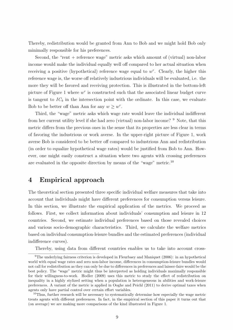
Thereby, redistribution would be granted from Ann to Bob and we might hold Bob only

minimally responsible for his preferences.

Second, the “rent + reference wage” metric asks which amount of (virtual) non-labor

income would make the individual equally well off compared to her actual situation when

receiving a positive (hypothetical) reference wage equal to wr. Clearly, the higher this

reference wage is, the worse off relatively industrious individuals will be evaluated, i.e. the

more they will be favored and receiving protection. This is illustrated in the bottom-left

picture of Figure 1 where wr is constructed such that the associated linear budget curve

is tangent to ICb in the intersection point with the ordinate. In this case, we evaluate

Bob to be better off than Ann for any w ≥ wr.

Third, the “wage” metric asks which wage rate would leave the individual indifferent

from her current utility level if she had zero (virtual) non-labor income? 9 Note, that this

metric differs from the previous ones in the sense that its properties are less clear in terms

of favoring the industrious or work averse. In the upper-right picture of Figure 1, work

averse Bob is considered to be better off compared to industrious Ann and redistribution

(in order to equalize hypothetical wage rates) would be justified from Bob to Ann. How-

ever, one might easily construct a situation where two agents with crossing preferences

are evaluated in the opposite direction by means of the “wage” metric.10

4 Empirical approach

The theoretical section presented three specific individual welfare measures that take into

account that individuals might have different preferences for consumption versus leisure.

In this section, we illustrate the empirical application of the metrics. We proceed as

follows. First, we collect information about individuals’ consumption and leisure in 12

countries. Second, we estimate individual preferences based on those revealed choices

and various socio-demographic characteristics. Third, we calculate the welfare metrics

based on individual consumption-leisure bundles and the estimated preferences (individual

indifference curves).

Thereby, using data from different countries enables us to take into account cross-

9The underlying fairness criterion is developed in Fleurbaey and Maniquet (2006): in an hypotheticalworld with equal wage rates and zero non-labor income, differences in consumption-leisure bundles wouldnot call for redistribution as they can only be due to differences in preferences and laisser-faire would be thebest policy. The “wage” metric might thus be interpreted as holding individuals maximally responsiblefor their willingness-to-work. Hodler (2009) uses this metric to study the effect of redistribution oninequality in a highly stylized setting when a population is heterogeneous in abilities and work-leisurepreferences. A variant of the metric is applied in Ooghe and Peichl (2011) to derive optimal taxes whenagents only have partial control over certain effort variables.

10Thus, further research will be necessary to systematically determine how especially the wage metrictreats agents with different preferences. In fact, in the empirical section of this paper it turns out that(on average) we are making more comparisons of the kind illustrated in Figure 1.

9

country differences in consumption-leisure preferences, i.e. preference profiles of different

populations besides the heterogeneity in individual tastes within a country. Addressing

these potential differences requires to keep other factors of the analysis (socio-demographic

variation, differences in the tax-benfit systems etc.) as comparable as possible. We there-

fore make use of a unique setting and estimate household preferences in a harmonized way

for all countries under analysis by using (a) comparable datasets with common variable

definitions, (b) a common econometric approach to estimate labor supply models for each

country and (c) a harmonized tax-benefit calculator to compute net incomes at different

points of the household budget curves as required by the nature of the labor supply model

and explained below. We also focus on a specific subgroup of the population, namely mar-

ried women. First, married women is the group most studied in the labor supply literature

as they show lots of variation in work duration and thus also relatively considerable dif-

ferences in labor supply elasticities (see e.g. Blundell and MaCurdy, 1999). Since this

variation partly is affected by differences in consumption-leisure preferences, it might also

help to identify differences in the empirical welfare measures. Second, married women’s

labor supply is less likely to be contaminated by demand-side restrictions compared to

single individuals or married men (Bargain et al, 2010), a factor not explicitly considered

with our approach (see below).

The empirical model is directly compatible with the theoretical framework presented

in the previous section. The only difference is that we consider “unitary” households

rather than individuals, i.e., couples are assumed to behave as a single decision maker

regarding the trade-off between consumption and female labor supply (male labor supply

is kept fixed).

Specification of preferences. In order to empirically derive the welfare metrics, we

must retrieve indifference curves for each household in our sample and, hence, estimate

utility functions. To do so, we specify a structural model of labor supply with discrete

choices, which is standard in the literature on tax reforms (see e.g. Aaberge et al, 1995;

Van Soest, 1995; Blundell et al, 2000).11 Agents are assumed to choose among a set

of discrete hours alternatives rather than continuously distributed options which better

corresponds to the observed distribution of available hours (non-participation and several

part-time, full-time and over-time categories). Also, a discrete choice model better allows

to account for the non-linear effect of tax-benefit systems on household budgets as net

income needs to be determined at each discrete point. Consumption-leisure preferences

are explicitly parameterized as follows while a common specification over all countries is

applied for reasons of comparability. We denote cij the net income (or consumption, in

11Relying on structural models is also the only way to obtain comparable preference estimates acrosscountries. It seems indeed difficult to find natural experiments that would allow performing this task.

10

a static framework) of household i and hij the wife’s working hours at choice j = 1, ..., J

where the household is assumed to obtain a utility level:

Vij = ui(cij, (T − hij)) + ϵij, (4)

with (T −hi) the wife’s “leisure time” (which may include time for domestic production),

i.e., total time-endowment T minus formal hours of work. For the deterministic part of

the utility function, we rely on a Box-Cox specification, that is:

ui(cij, (T − hij)) = βc

cαcij − 1

αc

+ βli(T − hij)

αl − 1

αl

. (5)

This specification is frequently used for welfare assessments (see e.g. Aaberge et al, 1995,

2000, 2004; Decoster and Haan, 2010; Aaberge and Colombino, 2011; Blundell and Shep-

hard, forthcoming). Importantly for our purpose, it is easy to check that monotonicity

and concavity conditions on consumption and leisure are satisfied (respectively βc > 0

and βli > 0 for monotonicity and αc < 1 and αl < 1 for concavity). Indeed, tangency

conditions are necessary for measuring and interpreting the welfare metrics in a straight-

forward way. The deterministic utility is completed by i.i.d. random terms ϵij for each

choice, leading to the individual random utility function Vij(ui, ϵij). By using a random

utility concept, we especially account for the fact that there will always be characteristics

of the household (influencing the hours choice) that are known by the household itself

while being unobserved by the econometrician. This specifically includes that for a given

household, tastes may vary across opportunities which will not be captured by estimat-

ing the deterministic part of the utility function (McFadden, 1974).12 As a consequence,

non-concavity of ui would not be inconsistent with random utility theory (as long as Vi is

quasi-concave). However, this restrictive assumption is necessary in order to empirically

derive (well-behaved) welfare metrics in line with the theory laid out in Section 3. This is

explained below where we suggest a way to empirically deal with this issue. In addition,

in Section 5.4, we check robustness with respect to a different, more flexible specification

of the utility function and to alternative ways to empirically compute the welfare metrics.

Under the (standard) assumption that random terms follow an extreme value type I

(EV-I) distribution, the probability for each household of choosing a given alternative has

an explicit logistic form, which is a function of deterministic utilities at all choices. Then,

the likelihood of a sample of observed choices can be derived from these probabilities

as a function of the preference parameters whose estimates are obtained by maximum

likelihood techniques (see McFadden, 1974).

12Besides, the random term might also capture possible observational errors, optimization errors ortransitory situations.

11

A crucial point for our analysis is the source of heterogeneity across households. The

first obvious difference is that α and β parameters are country-specific, i.e., they are esti-

mated separately for each country. The second source is household-specific heterogeneity

through the leisure term, which is specified as follows:

βli = βl0 + βlzzi, (6)

with zi a vector of taste shifters including the age of both spouses, education of the

women, presence of children younger than 3, between 3-6 or 7-12 years old and regional

information.

Note that we keep the labor supply model as simple as possible in order to ensure

a straightforward implementation and clear interpretation of the welfare metrics. This

particularly implies that we do not model potential demand side restrictions on the labor

market nor fixed costs of work. This is further discussed in Section 6.

Data, selection and tax-benefit simulation. For our empirical application, we focus

on a selection of 11 European countries and the US. For each country we use microdata

based on standard household surveys which provide information on incomes and demo-

graphics. For EU countries, we rely on datasets combined with the simulation of national

tax-benefit systems for years 1998 or 2001 as described in Bargain et al (2012). For the US,

we use 2006 IPUMS-CPS (Integrated Public Use Microdata Series; Current Population

Survey) data containing information for the year 2005. As mentioned above, we focus on

the subpopulation of married couples and estimate the labor supply of the women. Clearly,

this assumes away potential cross effects between labor supply decisions of the spouses.

However, given the illustrative purpose of the paper, this assumption seems acceptable.

To keep the sample relatively homogeneous and avoid too much variation in household’s

non-labor income (in this context especially including husbands’ labor income), we select

households where husbands at least work 30 hours/week and exclude those with extreme

amounts of capital income. Furthermore, we keep households where women are aged

between 18 and 59 and available for the labor market, i.e., neither disabled nor retired

nor in education. In order to maintain a comparable framework while respecting possible

variation in the hours distribution across countries, we adopt a discretization with J = 7

hours categories including non-participation, two part-time options, two full-time and two

over-time categories (0 to 60 hours/week with a step of 10 hours). Net income at each dis-

crete choice j = 1, ..., J is calculated as a function cij = f(wihij, Ii,xi) of female earnings

wihij and household non-labor income Ii (i.e., household capital income and husbands’

earnings. Female wages wi are predicted for all observations using calculated wage rates

of the workers and estimated with the usual correction for selection bias. The function

12

f(.) represents how gross income is transformed into net income, i.e., the impact of taxes

and benefits which also depends on certain household demographic characteristics xi.13

It is calculated numerically using microsimulation models EUROMOD for EU countries

and the NBER’s TAXSIM for the US.14

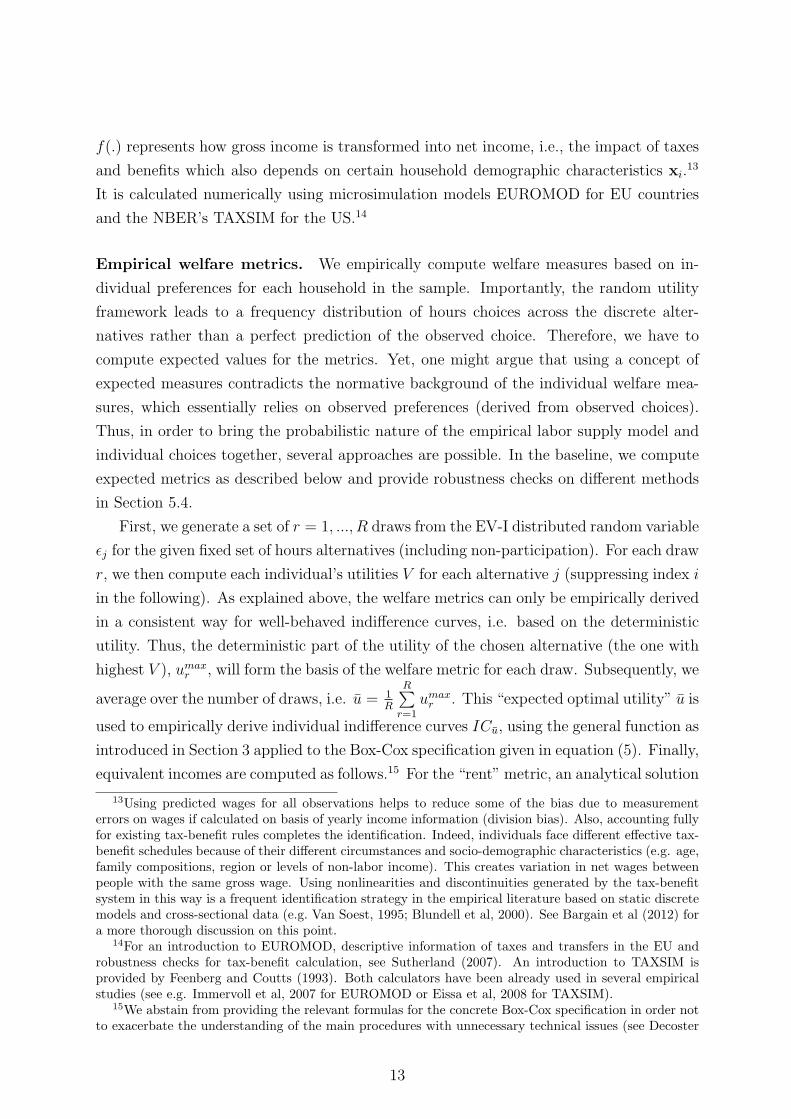
Empirical welfare metrics. We empirically compute welfare measures based on in-

dividual preferences for each household in the sample. Importantly, the random utility

framework leads to a frequency distribution of hours choices across the discrete alter-

natives rather than a perfect prediction of the observed choice. Therefore, we have to

compute expected values for the metrics. Yet, one might argue that using a concept of

expected measures contradicts the normative background of the individual welfare mea-

sures, which essentially relies on observed preferences (derived from observed choices).

Thus, in order to bring the probabilistic nature of the empirical labor supply model and

individual choices together, several approaches are possible. In the baseline, we compute

expected metrics as described below and provide robustness checks on different methods

in Section 5.4.

First, we generate a set of r = 1, ..., R draws from the EV-I distributed random variable

ϵj for the given fixed set of hours alternatives (including non-participation). For each draw

r, we then compute each individual’s utilities V for each alternative j (suppressing index i

in the following). As explained above, the welfare metrics can only be empirically derived

in a consistent way for well-behaved indifference curves, i.e. based on the deterministic

utility. Thus, the deterministic part of the utility of the chosen alternative (the one with

highest V ), umaxr , will form the basis of the welfare metric for each draw. Subsequently, we

average over the number of draws, i.e. u = 1R

R∑r=1

umaxr . This “expected optimal utility” u is

used to empirically derive individual indifference curves ICu, using the general function as

introduced in Section 3 applied to the Box-Cox specification given in equation (5). Finally,

equivalent incomes are computed as follows.15 For the “rent” metric, an analytical solution

13Using predicted wages for all observations helps to reduce some of the bias due to measurementerrors on wages if calculated on basis of yearly income information (division bias). Also, accounting fullyfor existing tax-benefit rules completes the identification. Indeed, individuals face different effective tax-benefit schedules because of their different circumstances and socio-demographic characteristics (e.g. age,family compositions, region or levels of non-labor income). This creates variation in net wages betweenpeople with the same gross wage. Using nonlinearities and discontinuities generated by the tax-benefitsystem in this way is a frequent identification strategy in the empirical literature based on static discretemodels and cross-sectional data (e.g. Van Soest, 1995; Blundell et al, 2000). See Bargain et al (2012) fora more thorough discussion on this point.

14For an introduction to EUROMOD, descriptive information of taxes and transfers in the EU androbustness checks for tax-benefit calculation, see Sutherland (2007). An introduction to TAXSIM isprovided by Feenberg and Coutts (1993). Both calculators have been already used in several empiricalstudies (see e.g. Immervoll et al, 2007 for EUROMOD or Eissa et al, 2008 for TAXSIM).

15We abstain from providing the relevant formulas for the concrete Box-Cox specification in order notto exacerbate the understanding of the main procedures with unnecessary technical issues (see Decoster

13

is obtained by setting h to zero into the formula for ICu and retrieving the corresponding

level of consumption (hence, the intersection level of ICu with the ordinate), see bottom-

right panel of Figure 1. Due to the Box-Cox specification of the deterministic utility we are

not able to derive analytical expressions for the other two metrics. Hence, we must apply

numerical procedures. This basically requires searching for the relevant tangency point

(c, h) of ICu with the hypothetical budget line corresponding to the metric of interest -

along the full shape of each individual indifference curve on the hours interval [0, T ] (while

this point, again, usually will be different from the observed bundle). Once the tangency

point (c, h) is found, the value for the metric is determined as well. More precisely, for the

“rent + reference wage” metric, the tangency point is the point (c, h) on ICu for which

the MRSc,h equals the reference wage wr. The virtual non-labor income µ corresponding

to this tangency point is the value for the metric (see bottom-left panel of Figure 1).

Finally, the “wage” metric is derived as the slope of ICu for which the MRSc,h, because

of the zero virtual non-labor income, equals ch(see top-right panel of Figure 1). For the

numerical derivation of the two last metrics, we rely on a precise iterative procedure by

incrementing hours from 0 to T for each household in the sample using very small steps

(0.01 hours/week). Note that this is different from moving across discrete categories

j = 1, ..., J as used for the labor supply estimation.

Descriptive information. In Table 1, we present summary statistics for the sample

under analysis. The first two columns show the average weekly household net and non-

labor income by countries (recall that household non-labor income essentially includes

husband’s earnings). Next, female average wage rates, weekly working hours as well

as participation rates are presented. Depending on the year of the data, incomes and

wages are up- or downrated to the reference year 2001 and transferred into comparable

Purchasing Power Parities (PPP)-USD.

Women from the US show the highest net wages per hour and clearly work more (27.2)

than average weekly hours across countries (24.7). Together with husbands’ earnings, this

results in the highest household net income on average per week in the sample (1158 PPP-

USD). However, females from the Nordic countries (Denmark, Finland, Sweden) show the

highest inclination to work (all above 30 hours/week and participation rates larger than

80%). Also, Portuguese married women, the well-known exception out of the Southern

European countries, tend to work more than US females - even though their wages are by

far the lowest across countries. In contrast, women from Germany, Ireland, Austria and

the Netherlands show relatively low participation rates and hours.

and Haan, 2010, for details). The reader may verify the proceeding directly via Figure 1 and the formulasintroduced in Section 3.

14

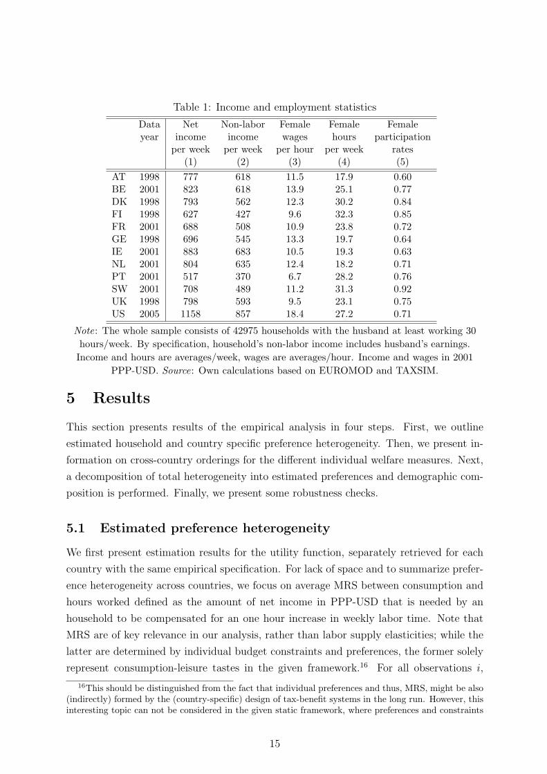
Table 1: Income and employment statistics

Data Net Non-labor Female Female Femaleyear income income wages hours participation

per week per week per hour per week rates(1) (2) (3) (4) (5)

AT 1998 777 618 11.5 17.9 0.60BE 2001 823 618 13.9 25.1 0.77DK 1998 793 562 12.3 30.2 0.84FI 1998 627 427 9.6 32.3 0.85FR 2001 688 508 10.9 23.8 0.72GE 1998 696 545 13.3 19.7 0.64IE 2001 883 683 10.5 19.3 0.63NL 2001 804 635 12.4 18.2 0.71PT 2001 517 370 6.7 28.2 0.76SW 2001 708 489 11.2 31.3 0.92UK 1998 798 593 9.5 23.1 0.75US 2005 1158 857 18.4 27.2 0.71

Note: The whole sample consists of 42975 households with the husband at least working 30

hours/week. By specification, household’s non-labor income includes husband’s earnings.

Income and hours are averages/week, wages are averages/hour. Income and wages in 2001

PPP-USD. Source: Own calculations based on EUROMOD and TAXSIM.

5 Results

This section presents results of the empirical analysis in four steps. First, we outline

estimated household and country specific preference heterogeneity. Then, we present in-

formation on cross-country orderings for the different individual welfare measures. Next,

a decomposition of total heterogeneity into estimated preferences and demographic com-

position is performed. Finally, we present some robustness checks.

5.1 Estimated preference heterogeneity

We first present estimation results for the utility function, separately retrieved for each

country with the same empirical specification. For lack of space and to summarize prefer-

ence heterogeneity across countries, we focus on average MRS between consumption and

hours worked defined as the amount of net income in PPP-USD that is needed by an

household to be compensated for an one hour increase in weekly labor time. Note that

MRS are of key relevance in our analysis, rather than labor supply elasticities; while the

latter are determined by individual budget constraints and preferences, the former solely

represent consumption-leisure tastes in the given framework.16 For all observations i,

16This should be distinguished from the fact that individual preferences and thus, MRS, might be also(indirectly) formed by the (country-specific) design of tax-benefit systems in the long run. However, thisinteresting topic can not be considered in the given static framework, where preferences and constraints

15

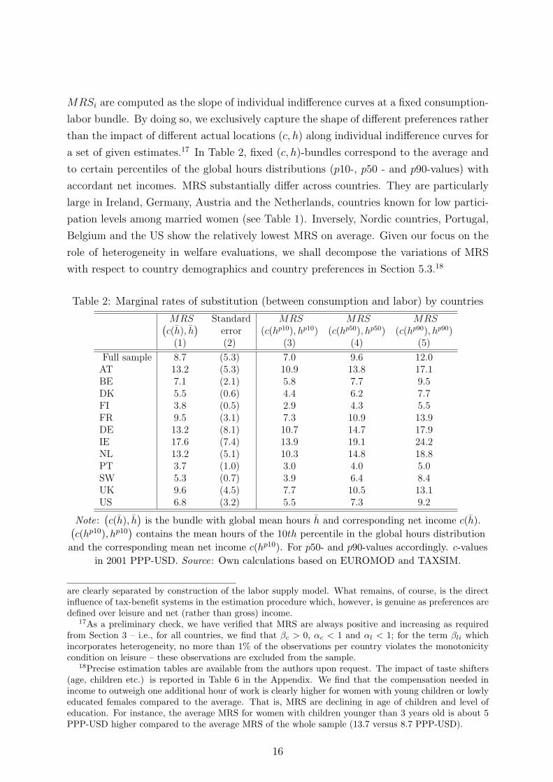
MRSi are computed as the slope of individual indifference curves at a fixed consumption-

labor bundle. By doing so, we exclusively capture the shape of different preferences rather

than the impact of different actual locations (c, h) along individual indifference curves for

a set of given estimates.17 In Table 2, fixed (c, h)-bundles correspond to the average and

to certain percentiles of the global hours distributions (p10-, p50 - and p90-values) with

accordant net incomes. MRS substantially differ across countries. They are particularly

large in Ireland, Germany, Austria and the Netherlands, countries known for low partici-

pation levels among married women (see Table 1). Inversely, Nordic countries, Portugal,

Belgium and the US show the relatively lowest MRS on average. Given our focus on the

role of heterogeneity in welfare evaluations, we shall decompose the variations of MRS

with respect to country demographics and country preferences in Section 5.3.18

Table 2: Marginal rates of substitution (between consumption and labor) by countries

MRS Standard MRS MRS MRS(c(h), h

)error (c(hp10), hp10) (c(hp50), hp50) (c(hp90), hp90)

(1) (2) (3) (4) (5)

Full sample 8.7 (5.3) 7.0 9.6 12.0AT 13.2 (5.3) 10.9 13.8 17.1BE 7.1 (2.1) 5.8 7.7 9.5DK 5.5 (0.6) 4.4 6.2 7.7FI 3.8 (0.5) 2.9 4.3 5.5FR 9.5 (3.1) 7.3 10.9 13.9DE 13.2 (8.1) 10.7 14.7 17.9IE 17.6 (7.4) 13.9 19.1 24.2NL 13.2 (5.1) 10.3 14.8 18.8PT 3.7 (1.0) 3.0 4.0 5.0SW 5.3 (0.7) 3.9 6.4 8.4UK 9.6 (4.5) 7.7 10.5 13.1US 6.8 (3.2) 5.5 7.3 9.2

Note:(c(h), h

)is the bundle with global mean hours h and corresponding net income c(h).(

c(hp10), hp10)contains the mean hours of the 10th percentile in the global hours distribution

and the corresponding mean net income c(hp10). For p50- and p90-values accordingly. c-values

in 2001 PPP-USD. Source: Own calculations based on EUROMOD and TAXSIM.

are clearly separated by construction of the labor supply model. What remains, of course, is the directinfluence of tax-benefit systems in the estimation procedure which, however, is genuine as preferences aredefined over leisure and net (rather than gross) income.

17As a preliminary check, we have verified that MRS are always positive and increasing as requiredfrom Section 3 – i.e., for all countries, we find that βc > 0, αc < 1 and αl < 1; for the term βli whichincorporates heterogeneity, no more than 1% of the observations per country violates the monotonicitycondition on leisure – these observations are excluded from the sample.

18Precise estimation tables are available from the authors upon request. The impact of taste shifters(age, children etc.) is reported in Table 6 in the Appendix. We find that the compensation needed inincome to outweigh one additional hour of work is clearly higher for women with young children or lowlyeducated females compared to the average. That is, MRS are declining in age of children and level ofeducation. For instance, the average MRS for women with children younger than 3 years old is about 5PPP-USD higher compared to the average MRS of the whole sample (13.7 versus 8.7 PPP-USD).

16

5.2 Cross-country welfare rankings

We first pool households from all countries into one sample and compare individual ranks

for the different metrics by use of correlation plots. Moving closer to country comparisons,

we then investigate how average country positions change by choice of the metric.

Rank correlations. For the pooled country sample, Figure 2 shows empirical rank

correlations between individual positions in the percentile distribution of the different

metrics. For the sake of comparison, the two upper panels show correlations when identical

preferences are assumed (instead of allowing for full heterogeneity). This corresponds to

the prominent approach in empirical welfare analysis described above. Precisely, for all

households in the pooled sample, we fix their preferences to that of the global median

household (in terms of MRSc(h),h) while retaining their actual (c, h)-choices and non-

preference related characteristics (net wages and non-labor income). The metrics are

recalculated under these conditions. As indicated in the upper-left panel of Figure 2, any

metric can be used at this stage without altering the correlation (which is independent

of the choice of the reference household and verified in the upper-right panel).19 Note

that overall reranking due to the account of leisure in the money metrics is fairly modest

when agents do not differ in preferences. This could of course vary with the choice of the

reference household and is checked in the robustness analysis in Section 5.4.

The next four panels of Figure 2 compare rank distributions for two measures at a time

when full heterogeneity in preferences is accounted for. We observe substantial reranking

of individual positions between the metrics. While the center-left panel of Figure 2 still

reveals a quite strong correlation between the individual positions under pure income and

the “rent” metric (similar to the upper-left picture), the correlation between the “rent”

and the further metrics in the following three panels sequentially decreases when taking

preferences for leisure increasingly into account. In the bottom-right panel, only a weak

correlation remains between the “rent” and the “wage” metric, showing the relatively

largest reranking between individual situations. The next paragraph analyzes to which

extent these rerankings affect cross-country orderings of individual welfare.

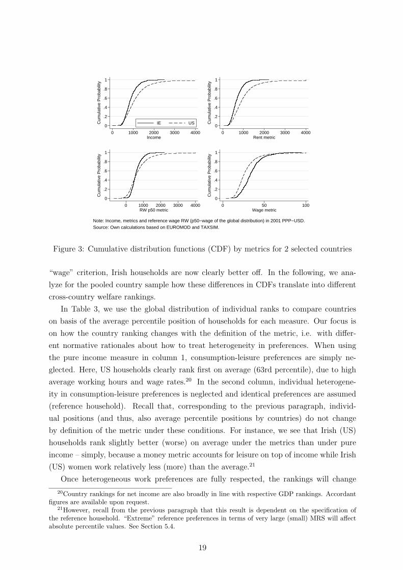
Welfare rankings. As a preliminary exercise, we compare cumulative distribution func-

tions (CDF) of the different metrics for two illustrative countries, namely the US and Ire-

land. The upper-left panel of Figure 3 shows that US households are relatively better off

in terms of income or under the “rent” criterion. However, moving to the “rent+reference

wage” metric, CDFs start to cross and households from the US become worse off. For the

19Indeed, this illustrates nothing else than what Roberts (1980) proved, namely, that individual welfareorderings are reference price independent when preferences are homogeneous across individuals.

17

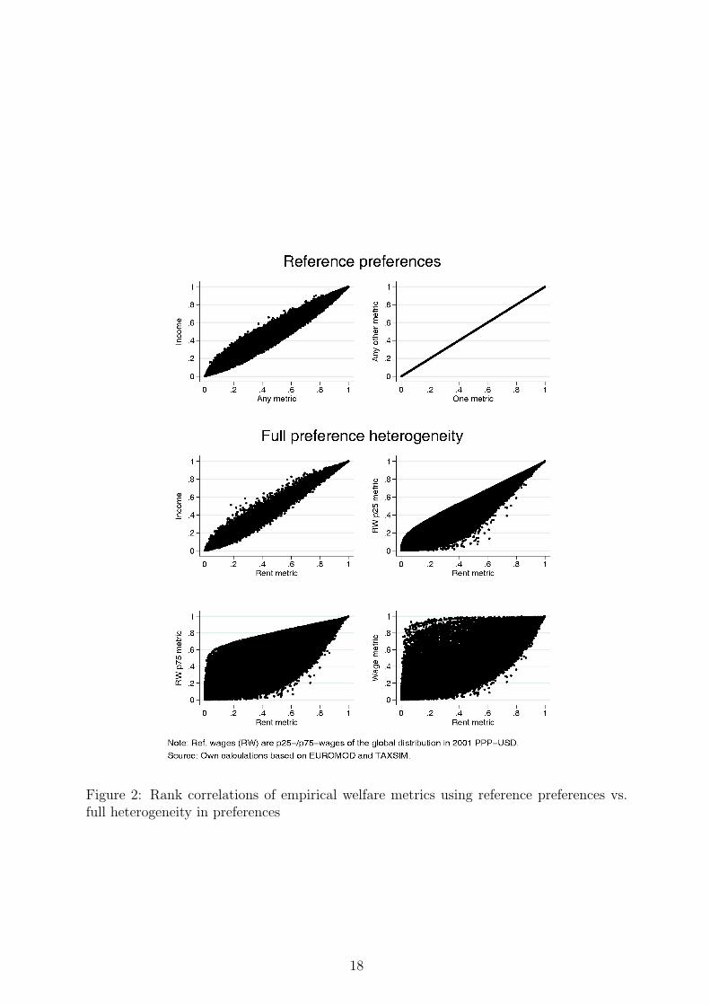
Figure 2: Rank correlations of empirical welfare metrics using reference preferences vs.full heterogeneity in preferences

18

0

.2

.4

.6

.8

1

Cum

ulat

ive

Pro

babi

lity

0 1000 2000 3000 4000Income

IE US0

.2

.4

.6

.8

1

Cum

ulat

ive

Pro

babi

lity

0 1000 2000 3000 4000Rent metric

0

.2

.4

.6

.8

1

Cum

ulat

ive

Pro

babi

lity

0 1000 2000 3000 4000RW p50 metric

0

.2

.4

.6

.8

1

Cum

ulat

ive

Pro

babi

lity

0 50 100Wage metric

Note: Income, metrics and reference wage RW (p50−wage of the global distribution) in 2001 PPP−USD.Source: Own calculations based on EUROMOD and TAXSIM.

Figure 3: Cumulative distribution functions (CDF) by metrics for 2 selected countries

“wage” criterion, Irish households are now clearly better off. In the following, we ana-

lyze for the pooled country sample how these differences in CDFs translate into different

cross-country welfare rankings.

In Table 3, we use the global distribution of individual ranks to compare countries

on basis of the average percentile position of households for each measure. Our focus is

on how the country ranking changes with the definition of the metric, i.e. with differ-

ent normative rationales about how to treat heterogeneity in preferences. When using

the pure income measure in column 1, consumption-leisure preferences are simply ne-

glected. Here, US households clearly rank first on average (63rd percentile), due to high

average working hours and wage rates.20 In the second column, individual heterogene-

ity in consumption-leisure preferences is neglected and identical preferences are assumed

(reference household). Recall that, corresponding to the previous paragraph, individ-

ual positions (and thus, also average percentile positions by countries) do not change

by definition of the metric under these conditions. For instance, we see that Irish (US)

households rank slightly better (worse) on average under the metrics than under pure

income – simply, because a money metric accounts for leisure on top of income while Irish

(US) women work relatively less (more) than the average.21

Once heterogeneous work preferences are fully respected, the rankings will change

20Country rankings for net income are also broadly in line with respective GDP rankings. Accordantfigures are available upon request.

21However, recall from the previous paragraph that this result is dependent on the specification ofthe reference household. “Extreme” reference preferences in terms of very large (small) MRS will affectabsolute percentile values. See Section 5.4.

19

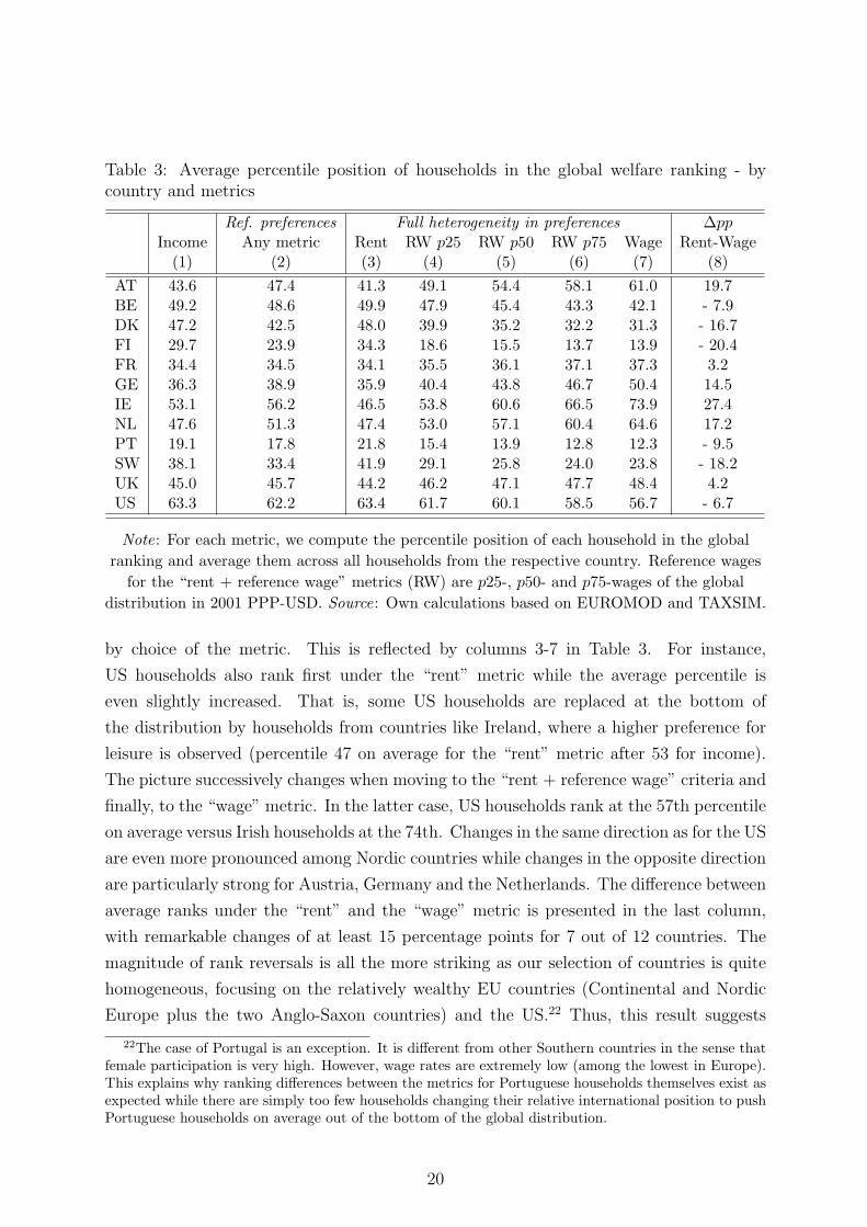
Table 3: Average percentile position of households in the global welfare ranking - bycountry and metrics

Ref. preferences Full heterogeneity in preferences ∆ppIncome Any metric Rent RW p25 RW p50 RW p75 Wage Rent-Wage(1) (2) (3) (4) (5) (6) (7) (8)

AT 43.6 47.4 41.3 49.1 54.4 58.1 61.0 19.7BE 49.2 48.6 49.9 47.9 45.4 43.3 42.1 - 7.9DK 47.2 42.5 48.0 39.9 35.2 32.2 31.3 - 16.7FI 29.7 23.9 34.3 18.6 15.5 13.7 13.9 - 20.4FR 34.4 34.5 34.1 35.5 36.1 37.1 37.3 3.2GE 36.3 38.9 35.9 40.4 43.8 46.7 50.4 14.5IE 53.1 56.2 46.5 53.8 60.6 66.5 73.9 27.4NL 47.6 51.3 47.4 53.0 57.1 60.4 64.6 17.2PT 19.1 17.8 21.8 15.4 13.9 12.8 12.3 - 9.5SW 38.1 33.4 41.9 29.1 25.8 24.0 23.8 - 18.2UK 45.0 45.7 44.2 46.2 47.1 47.7 48.4 4.2US 63.3 62.2 63.4 61.7 60.1 58.5 56.7 - 6.7

Note: For each metric, we compute the percentile position of each household in the global

ranking and average them across all households from the respective country. Reference wages

for the “rent + reference wage” metrics (RW) are p25-, p50- and p75-wages of the global

distribution in 2001 PPP-USD. Source: Own calculations based on EUROMOD and TAXSIM.

by choice of the metric. This is reflected by columns 3-7 in Table 3. For instance,

US households also rank first under the “rent” metric while the average percentile is

even slightly increased. That is, some US households are replaced at the bottom of

the distribution by households from countries like Ireland, where a higher preference for

leisure is observed (percentile 47 on average for the “rent” metric after 53 for income).

The picture successively changes when moving to the “rent + reference wage” criteria and

finally, to the “wage” metric. In the latter case, US households rank at the 57th percentile

on average versus Irish households at the 74th. Changes in the same direction as for the US

are even more pronounced among Nordic countries while changes in the opposite direction

are particularly strong for Austria, Germany and the Netherlands. The difference between

average ranks under the “rent” and the “wage” metric is presented in the last column,

with remarkable changes of at least 15 percentage points for 7 out of 12 countries. The

magnitude of rank reversals is all the more striking as our selection of countries is quite

homogeneous, focusing on the relatively wealthy EU countries (Continental and Nordic

Europe plus the two Anglo-Saxon countries) and the US.22 Thus, this result suggests

22The case of Portugal is an exception. It is different from other Southern countries in the sense thatfemale participation is very high. However, wage rates are extremely low (among the lowest in Europe).This explains why ranking differences between the metrics for Portuguese households themselves exist asexpected while there are simply too few households changing their relative international position to pushPortuguese households on average out of the bottom of the global distribution.

20

that heterogeneous consumption-leisure preferences are the driving factor for individual

rerankings across countries. In addition, note that international rankings are affected by

population size, which may even limit the extent of rank reversals for large countries. The

same is true for natural differences in household non-labor income (husband’s earnings)

and female wages across countries (given individual choices).23

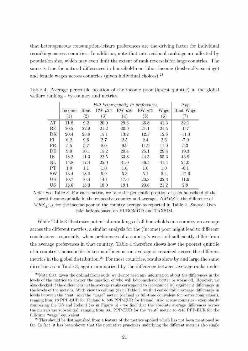
Table 4: Average percentile position of the income poor (lowest quintile) in the globalwelfare ranking - by country and metrics

Full heterogeneity in preferences ∆ppIncome Rent RW p25 RW p50 RW p75 Wage Rent-Wage(1) (2) (3) (4) (5) (6) (7)

AT 11.8 9.2 20.9 29.6 36.8 41.3 32.1BE 20.5 22.2 21.2 20.9 21.1 21.5 -0.7DK 20.4 23.9 15.1 13.2 12.3 12.6 -11.3FI 6.2 9.6 2.7 2.5 2.4 2.6 -7.0FR 5.5 5.7 8.0 9.9 11.9 11.0 5.3DE 9.0 10.1 15.2 20.4 25.1 29.4 19.3IE 18.2 11.3 22.5 33.8 44.5 55.3 43.9NL 15.8 17.4 25.0 31.0 36.5 41.4 24.0PT 1.0 1.1 1.0 1.0 1.0 1.0 -0.1SW 13.4 18.0 5.9 5.3 5.1 5.4 -12.6UK 10.7 10.4 14.1 17.6 20.8 22.3 11.9US 18.6 18.3 18.0 19.1 20.6 21.2 2.9

Note: See Table 3. For each metric, we take the percentile position of each household of the

lowest income quintile in the respective country and average. ∆MRS is the difference of

MRSc(h),h for the income poor to the country average as reported in Table 2. Source: Own

calculations based on EUROMOD and TAXSIM.

While Table 3 illustrates potential rerankings of all households in a country on average

across the different metrics, a similar analysis for the (income) poor might lead to different

conclusions - especially, when preferences of a country’s worst-off sufficiently differ from

the average preferences in that country. Table 4 therefore shows how the poorest quintile

of a country’s households in terms of income on average is reranked across the different

metrics in the global distribution.24 For most countries, results show by and large the same

direction as in Table 3, again summarized by the difference between average ranks under

23Note that, given the ordinal framework, we do not need any information about the differences in thelevels of the metrics to answer the question of who will be considered better or worse off. However, wealso checked if the differences in the average ranks correspond to (economically) significant differences inthe levels of the metrics. With view to column (8) in Table 3, we find considerable average differences inlevels between the “rent” and the “wage” metric (defined as full-time equivalent for better comparison),ranging from 18 PPP-EUR for Finland to 695 PPP-EUR for Ireland. Also across countries - exemplarilycomparing the US and Ireland (as in Figure 3) - we find that the absolute average differences acrossthe metrics are substantial, ranging from 331 PPP-EUR for the “rent” metric to -245 PPP-EUR for thefull-time “wage” equivalent.

24This should be distinguished from a feature of the metrics applied which has not been mentioned sofar. In fact, it has been shown that the normative principles underlying the different metrics also single

21

the “rent” and the “wage” metric in the last column. The extent of rerankings, however,

differs. For instance, the income poor in Portugal find themselves in the lowest percentile

of the global distribution and thus, unsurprisingly fare also worst under the remaining

metrics, with a marginal improvement for the “rent” metric only. Contrary, rerankings

are even more significant for households from countries with a relatively lower preference

for work, as e.g. Ireland. For Belgium, there is barely an effect and most interestingly,

the ranking of the poor in the US changes in the opposite direction compared to Table

3. These effects might be somewhat explained with view to Table 7 in the Appendix,

revealing clearly higher MRS for this group in both countries compared to the average.

Interpretation. As explained in Section 3, the metrics applied differ only in the way

they treat heterogeneity in consumption-leisure preferences. As a result, agents with dif-

ferent willingness-to-work might be evaluated very differently depending on the metric.

Then, the first and most important question is, who will be considered better and worse off

under the various criteria. Therefore, we focused on a pure index ordering for each metric

based on individual percentile positions in the accordant global distribution. In terms of

country comparisons, we may cluster households according to certain groups of countries.

For instance, households from apparently “work-loving countries” (as Denmark and the

US) are better off on average than households from apparently “work-averse nations”

(e.g., Austria and Ireland) under the “rent” criterion. The reason is that with the “rent”

metric, the policy maker tends to evaluate an agent with a higher willingness-to-work to

be better off compared to another agent with a lower willingness-to-work (assigning low

responsibility for work aversion). Thus, the latter would eventually be favored to receive

redistribution from the former and on average, we make more interpersonal comparisons

of this sort “favoring” households from Ireland rather than from the US. Contrary, under

the “wage” metric, we obviously more often favor households from the US over those

from Ireland (due to maximal responsibility assigned to work aversion). However, these

considerations are based on the average percentiles for all households while we might con-

clude differently when looking at subgroups (income quintiles) of a countries population,

as additionally considered in the previous paragraph.

out a specific way of how to aggregate them, namely using a maximin (leximin) social welfare functionwith infinite aversion to inequality and thus, focusing on the worst-off (Fleurbaey, 2008). Again, as thispaper is about interpersonal comparisons and not about social evaluation, we do not consider any typeof an aggregator function for our analysis. However, looking at how the poor of each country fare in theworld distribution might be worth for answering the question of who will be better or worse off underwhich metric.

22

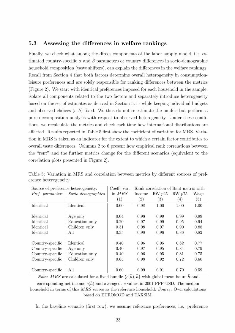
5.3 Assessing the differences in welfare rankings

Finally, we check what among the direct components of the labor supply model, i.e. es-

timated country-specific α and β parameters or country differences in socio-demographic

household composition (taste shifters), can explain the differences in the welfare rankings.

Recall from Section 4 that both factors determine overall heterogeneity in consumption-

leisure preferences and are solely responsible for ranking differences between the metrics

(Figure 2). We start with identical preferences imposed for each household in the sample,

isolate all components related to the two factors and separately introduce heterogeneity

based on the set of estimates as derived in Section 5.1 - while keeping individual budgets

and observed choices (c, h) fixed. We thus do not re-estimate the models but perform a

pure decomposition analysis with respect to observed heterogeneity. Under these condi-

tions, we recalculate the metrics and check each time how international distributions are

affected. Results reported in Table 5 first show the coefficient of variation for MRS. Varia-

tion in MRS is taken as an indicator for the extent to which a certain factor contributes to

overall taste differences. Columns 2 to 6 present how empirical rank correlations between

the “rent” and the further metrics change for the different scenarios (equivalent to the

correlation plots presented in Figure 2).

Table 5: Variation in MRS and correlation between metrics by different sources of pref-erence heterogeneity

Source of preference heterogeneity: Coeff. var. Rank correlation of Rent metric withPref. parameters Socio-demographics in MRS Income RW p25 RW p75 Wage

(1) (2) (3) (4) (5)

Identical Identical 0.00 0.98 1.00 1.00 1.00

Identical Age only 0.04 0.98 0.99 0.99 0.99Identical Education only 0.20 0.97 0.99 0.95 0.94Identical Children only 0.31 0.98 0.97 0.90 0.88Identical All 0.35 0.98 0.96 0.86 0.82

Country-specific Identical 0.40 0.96 0.95 0.82 0.77Country-specific Age only 0.40 0.97 0.95 0.84 0.79Country-specific Education only 0.40 0.96 0.95 0.81 0.75Country-specific Children only 0.65 0.98 0.92 0.72 0.60

Country-specific All 0.60 0.99 0.91 0.70 0.59

Note: MRS are calculated for a fixed bundle(c(h), h

)with global mean hours h and

corresponding net income c(h) and averaged. c-values in 2001 PPP-USD. The median

household in terms of this MRS serves as the reference household. Source: Own calculations

based on EUROMOD and TAXSIM.

In the baseline scenario (first row), we assume reference preferences, i.e. preference

23

parameters and characteristics are taken from the median MRS household as defined

above.25 The coefficient of variation for MRS equals zero by construction and the cor-

relation between the “rent” metric and income equals 0.98, while being perfect for the

other metrics (which corresponds to the aforementioned results in the top panels of Figure

2). Rows 2-5 introduce heterogeneity in socio-demographic characteristics. That is, all

preference parameters are held constant according to the reference household but some

characteristics are allowed to change across countries and households. In row 2, age dif-

ferences are the only source of variation. Obviously, this cannot explain much of the

variation in MRS and leaves the empirical correlations across metrics barely unchanged.

Education levels and especially the presence of children seem to explain more of the varia-

tion in MRS (rows 3 and 4); as a result, rank correlations between income and the metrics

become weaker when moving towards the “wage” metric. These effects cumulate when

heterogeneity in all three characteristics is allowed (row 5).

In rows 6-9, country-specific differences in preferences are considered. First, all socio-

demographic characteristics are kept constant and only differences in estimated preference

parameters determine heterogeneity in tastes. That is, α and β parameters are the only

source of variation across countries while characteristics zi are set according to the refer-

ence household. The magnitude of the effect is very similar to that of accounting for all

socio-demographic characteristics in the case before. Thus, country-specific consumption-

leisure preferences already explain a good deal of the observed variation in MRS and be-

tween the metrics. Second, country differences in socio-demographics are combined with

variation in different characteristics in rows 7-9. Here, especially the presence of young

children has a substantial impact on the variation across countries, which seems to account

for most of the variation when allowing for full heterogeneity in characteristics and esti-

mated preference parameters (last row). A standard variance decomposition (ANOVA)

for MRS and differences in individual ranks across metrics supports these findings. That

is, country-specific preferences as well as the correlation between country-specific prefer-

ences and family size (children) are most important and significant factors of variation

(detailed results are available upon request).

While the results presented so far only give an intuition about what affects overall

correlation between the ordinal metrics, nothing is said yet about which factors actually

drive the observed differences in individual cross-country rankings. Therefore, we addi-

tionally reproduce welfare rankings, again in terms of average percentiles, for the two main

counterfactual scenarios reflecting the different sources of heterogeneity. In the Appendix,

Table 8(a) only maintains differences in socio-demographic characteristics while in Table

25Note that results will depend on the choice of the reference household, why they should also atthis stage be considered as illustrative. However, we check for different specifications of the referencehousehold in Section 5.4.

24

8(b), only the heterogeneity in preference parameters is accounted for. As can be seen,

the differences between metrics and across countries in Table 8(b) are by and large similar

to the orderings in Table 3. In contrast, Table 8(a) only reveals a very small influence of

demographics on average ranking positions. This confirms the intuition from the previous

results that the ranking of individuals across countries in Table 3 is primarily affected by

estimated country-specific preferences (rather than by demographic composition).26

5.4 Robustness checks

In this section, we perform robustness checks with respect to the labor supply specification,

the calculation of the empirical welfare metrics and the decomposition analysis.

Labor supply model. For the illustrative purpose of this paper, an interpretationally

simple specification for the labor supply model has been used. A Box-Cox specification for

the deterministic part of the utility function – as often used in the normative literature

– seemed particularly suitable since monotonicity and concavity conditions are usually

fulfilled which can easily be checked ex-post. Using a more flexible functional form (e.g.

quadratic, see Bargain et al, 2012) is more frequent in the empirical literature on labor

supply and taxation. However, notice that the gains from flexibility are partly lost in the

present context given that tangency conditions must be imposed (which can be done by

adding monotonicity and concavity requirements as constraints directly into the likelihood

maximization). This is checked for the countries under analysis using the same data.

Results are summarized in Figure 4 in the Appendix, which plots different average MRS

as defined in Table 2 for the Box-Cox versus a (constrained) quadratic specification for

the labor supply model. Results are very similar and especially country rankings in terms

of MRS are mainly preserved. 27

Calculation of welfare metrics. We calculate welfare metrics by using indifference

curves based on estimated preference parameters and corresponding to a certain level

of utility. In the baseline, this level of welfare is taken as the expected value over a

large number of draws for the EV-I random terms (while always taking the resulting

optimal level of utility). However, alternative ways of computation can be suggested,

also consistent with the random nature of the labor supply model. First, metrics for

each optimal utility level of each draw are computed while averaging then follows over all

26There are few exceptions. For France, the trend in Table 3 is more similar to Table 8(a), suggestingthat the demographic composition drives the result for this country. Also Belgium shows a reverseinfluence of demographics, which, however, does not outweigh the impact of estimated preferences.

27Starting with 7 hours choices for both specifications as described above, we also find that estimationresults are robust to choosing an even narrower choice set with 13 categories (0 to 60 hours/week with astep of 5 hours). See also Bargain et al (2012).

25

calculated metric values (for each individual) rather than utilities. Second, we compute

the metrics for the utility level corresponding to each discrete hours category and directly

take the weighted sum (by predicted probabilities using the expected random term) -

rather then artificially drawing many random terms. While these alternative procedures

necessarily change the levels of the metrics, we find that they basically do not affect the

resulting orderings compared to the baseline results. This is shown in Figure 5 in the

Appendix where average percentile positions by countries are plotted for the baseline

method 1 (denoted “expected utility”) against methods 2 (denoted “expected metrics”)

and 3 (denoted “probabilities”).

Specification of the reference household. For the decomposition analysis in Section

5.3, the reference household in the baseline scenario was specified according to the me-

dian MRSc(h),h. However, variation in MRS and, hence, correlation between the metrics

when partly introducing preference heterogeneity, might be sensitive to that specifica-

tion. Thus, as a robustness check, further specifications for the reference household have

been set with respect to p10-, (p50-) and p90-values in the global distribution of MRS

(net income c). Table 9 shows that there is sufficient heterogeneity across the reference

households selected, both in terms of the country they stem from and in terms of socio-

demographic characteristics. Average MRS, the coefficient of variation for MRS and

correlation between the metrics of course change quantitatively with the specification.

Yet, our core results do not change, i.e. the finding that estimated country-specific pref-

erence parameters (rather then socio-demographic differences) determine heterogeneity in

the rankings across metrics and countries is confirmed. Figures 6 and 7 in the Appendix

plot average percentiles under the “rent” against the ”RW p50“ and the “wage” metric

- by different specifications of the reference household and for the two main scenarios

corresponding to Table 8. Clearly, Figure 7 (where heterogeneity is only due to estimated

preference parameters) shows remarkable variation of country average percentiles across

the different metrics while this is not true for Figure 6 (where heterogeneity is only due

to socio-demographic characteristics). Again, also absolute values for average percentiles

are affected by the choice of the reference household, however, relative differences in the

country rankings are basically preserved.

6 Concluding discussion

The aim of this paper was to contribute to the ‘beyond GDP’-debate in terms of inter-

personally comparing well-being in several dimensions and across different countries. We

have departed from standard income rankings by the inclusion of leisure, hence, respect-

ing one of the most primary specifications of welfare in the normative literature. Our

26

main focus was to illustrate for the consumption-leisure space the use of welfare metrics

that take preference heterogeneity into account. Our results suggest that differences in

consumption-leisure preferences – and their normative treatment – might matter sub-

stantially when interpersonally evaluating welfare in an international context. Precisely,

households from apparently “work-loving countries” (e.g. the US or Denmark) rank higher

on average under criteria that evaluate agents with a higher willingness-to-work to be bet-

ter off compared to agents with a lower willingness-to-work. Inversely, households from

the more “work-averse nations”(e.g. Austria or Ireland) are on top of the ranking on

average with a metric that considers agents with a relatively lower willingness-to-work as

better off. The reranking of households between nations when moving from the former

to the latter types of welfare criteria is substantial, which is noticeable given that we

consider a relatively homogeneous set of countries and since the welfare measures only

add one dimension to income (“leisure”). A decomposition analysis showed that cross-

country differences in consumption-leisure preferences are driving this result. However,

these statements, formulated on basis of the normative background of the metrics ap-

plied, should be solely understood in terms of interpersonal comparisons; the application

to social criteria and actual cross-country redistribution is left for future research.

For the sake of illustration and implementation of the welfare metrics, we intended to

keep the empirical framework of this paper simple. Hence, a lot remains to be done to

bring empirical estimations closer to the possibility of sound normative evaluations. In

particular, the fit of labor supply models is often improved by the introduction of a term

accounting for fixed costs of work. Thus it is possible to rationalize the non-participation

of some people in terms of fixed costs rather than through steep indifference curves –

and introducing fixed costs would certainly reduce some of the apparent differences in

MRS across household types and countries. However, fixed costs of work are usually not

identified from preferences, as shown by Van Soest et al (2002), but, if introduced in the

model, they may in fact capture some elements of work disutility (or even work utility, i.e.,

negative fixed costs, if inactivity is a source of despair, as shown by Clark and Oswald,

1994). A similar logic applies to demand-side constraints which restrict the choice set

available to the individual (Dagsvik, 1994; Aaberge et al, 1999; Dagsvik and Strøm, 2006)

and could also result in involuntary unemployment (Peichl and Siegloch, 2012). Here, a

specific and additionally demanding requirement in the present context would have been

to determine country-specific choice opportunities. In addition, one limitation of the mi-

crosimulation models we use is that in-kind benefits or public services more generally

are not taken into account due to data limitations. As the levels of non-cash transfers

differ across countries, this has implications for cross-country differences in welfare met-

rics. However, it is hard to assess ex-ante how accounting for public services would affect

the estimation of consumption-leisure preferences and hence the different welfare rank-

27

ings. Importantly, the construction and especially interpretation of welfare metrics as

used in the present paper is clearly more complicated when additionally accounting for

the various factors mentioned, i.e., especially in presence of non-regular and possibly dis-

continuous indifference curves. We leave these considerations for further research. Also,

we have chosen to model married women’s labor supply since variability in work hours

of this group is more likely to reflect true choices in the consumption-leisure space (and

responses to financial incentives) compared to other groups. Of course, a more complete

welfare analysis across countries should first include other subgroups as well and second,

consider further dimensions of individual well-being besides income and leisure. Finally,

comprehensive international welfare comparisons might also involve further aspects as

the respect for different population sizes or intertemporal comparisons (Fleurbaey and

Tadenuma, 2009).

References

Aaberge R, Colombino U (2011) Empirical Optimal Income Taxation: A Microeconomet-

ric Application to Norway. CHILD Working Paper No. 16/2011

Aaberge R, Dagsvik J, Strøm S (1995) Labor Supply Responses and Welfare Effects of

Tax Reforms. Scandinavian Journal of Economics 97(4):635–659

Aaberge R, Colombino U, Strøm S (1999) Labor Supply in Italy: An Empirical Analysis

of Joint Household Decisions, with Taxes and Quantity Constraints. Journal of Applied

Econometrics 14(4):403–422

Aaberge R, Colombino U, Strøm S (2000) Labor Supply Responses and Welfare Effects

from Replacing Current Tax Rules by a Flat Tax: Empirical Evidence from Italy,

Norway and Sweden. Journal of Population Economics 13(4):595–621

Aaberge R, Colombino U, Strøm S (2004) Do more equal slices shrink the cake? An

empirical investigation of tax-transfer reform proposals in Italy. Journal of Population

Economics 17:767–785

Alesina A, Glaeser E, Sacerdote B (2005) Work and Leisure in the United States and

Europe: Why So Different? NBER Macroeconomics Annual 20:1–64

Atkinson AB (2011) The Restoration of Welfare Economics. American Economic Review:

Papers and Proceedings 101(3):157–161

Bargain O, Caliendo M, Haan P, Orsini K (2010) Making Work Pay’ in a Rationed Labour

Market. Journal of Population Economics 21(1):323–351

28

Bargain O, Orsini K, Peichl A (2012) Comparing Labor Supply Elasticities in Europe and

the US: New Results. IZA Discussion Paper No. 6735

Becker GS, Philipson TJ, Soares RR (2005) The Quantity and Quality of Life and the

Evolution of World Inequality. Amercian Economic Review 95:277–291

Blackorby C, Donaldson D (1988) Money Metric Utility: A Harmless Normalization?

Journal of Economic Theory 46:120–129

Blackorby C, Laisney F, Schmachtenberg R (1993) Reference-price-independent welfare

prescriptions. Journal of Public Economics 50:63–76

Blanchard O (2004) The Economic Future of Europe. Journal of Economic Perspectives

18:3–26

Blundell R, MaCurdy T (1999) Labor Supply: A Review of Alternative Approaches.

In: Ashenfelter O, Card D (eds) Handbook of Labor Economics, Vol. 3A, Elsevier,

Amsterdam, pp 1559–1695

Blundell R, Shephard A (forthcoming) Employment, Hours of Work and the Optimal

Taxation of Low Income Families. Review of Economic Studies

Blundell R, Duncan A, McCrae J, Meghir C (2000) The Labour Market Impact of the

Working Families’ Tax Credit. Fiscal Studies 21(1):75–104

Brun BC, Tungodden B (2004) Non-welfaristic theories of justice: Is ”the intersection

approach” a solution to the indexing impasse? Social Choice and Welfare 22:49–60

Clark AE, Oswald AJ (1994) Unhappiness and Unemployment. Economic Journal

104(424):648–659

Creedy J, Herault N (2012) Welfare-improving income tax reforms: a microsimulation

analysis. Oxford Economic Papers 64(1):128–150

Dagsvik J (1994) Discrete and Continuous Choice, Max-Stable Processes, and Indepen-

dence from Irrelevant Attributes. Econometrica 62(5):1179–1205

Dagsvik J, Strøm S (2006) Sectoral Labor Supply, Choice Restrictions and Functional

Form. Journal of Applied Econometrics 21(6):803–826

Dagsvik J, Locatelli M, Strøm S (2009) Tax Reform, Sector-specific Labor Supply and

Welfare Effects. Scandinavian Journal of Economics 111(2):299–321

Decoster A, Haan P (2010) Empirical welfare analysis in random utility models of labour

supply. KU Leuven, CES Discussion Paper Series 10.30

29

Eissa N, Hoynes HW (2004) Taxes and the labor market participation of married couples:

the earned income tax credit. Journal of Public Economics 88(9-10):1931–1958

Eissa N, Kleven HJ, Kreiner C (2008) Evaluation of Four Tax Reforms in the United

States: Labor Supply and Welfare Effects for Single Mothers. Journal of Public Eco-

nomics 92:795–816

Ericson P, Flood L (2009) A Microsimulation Approach to an Optimal Swedish Income

Tax. IZA Discussion Paper No. 4379

Feenberg DR, Coutts E (1993) An Introduction to the TAXSIM Model. Journal of Policy

Analysis and Management 12(1):189–194

Fleurbaey M (2006) Social welfare, priority to the worst-off and the dimensions of indi-

vidual well-being. In: Farina F, Savaglio E (eds) Inequality and Economic Integration,

London: Routledge

Fleurbaey M (2007) Social choice and the indexing dilemma. Social Choice and Welfare

29:633–648

Fleurbaey M (2008) Fairness, Responsibility and Welfare. Oxford University Press

Fleurbaey M (2009) Beyond GDP: The Quest for a Measure of Social Welfare. Journal of

Economic Literature 47:1029–1075

Fleurbaey M (2011) Willingness-to-pay and the equivalence approach. Revue d’conomie

politique 121(1):35–58

Fleurbaey M, Gaulier G (2009) International Comparisons of Living Standards by Equiv-

alent Incomes. Scandinavian Journal of Economics 111:597–624

Fleurbaey M, Maniquet F (2006) Fair Income Tax. Review of Economic Studies 73(1):55–

83

Fleurbaey M, Tadenuma K (2009) Universal Social Orderings. CCES Discussion Paper

Series, No.9

Fleurbaey M, Trannoy A (2003) The Impossibility of a Paretian Egalitarian. Social Choice

and Welfare 21:243–263

Fuest C, Peichl A, Schaefer T (2008) Is a flat tax reform feasible in a grown-up democracy

of Western Europe? A simulation study for Germany. International Tax and Public

Finance 15(5):620–636

30

Hodler R (2009) Redistribution and Inequality in a Heterogeneous Society. Economica

76:704–718

Immervoll H, Kleven H, Kreiner C, Saez E (2007) Welfare Reform in European Countries:

A Micro-Simulation Analysis. The Economic Journal 117(516):1–44

Jones CI, Klenow PJ (2010) Beyond GDP? Welfare across Countries and Time. NBER

Working Paper 16352

Kassenboehmer SC, Schmidt CM (2011) Beyond GDP and Back: What is the Value-

Added by Additional Components of Welfare Measurement? IZA Discussion Paper No.

5453

King M (1983) Welfare effects of tax reforms using household data. Journal of Public

Economics 21:183–214

McFadden D (1974) Conditional Logit Analysis of Qualitative Choice Behavior. In:

Zarembka P (ed) Frontiers in Econometrics, Academic Press, New York, pp 105–142

Ooghe E, Peichl A (2011) Fair and Efficient Taxation under Partial Control: Theory and

Evidence. CESifo Working Paper No. 3518

Peichl A, Siegloch S (2012) Accounting for Labor Demand Effects in Structural Labor

Supply Models. Labour Economics 19(1):129–138

Pencavel J (1977) Constant-Utility Index Numbers of Real Wages. The American Eco-

nomic Review 67(2):91–100

Prescott EC (2004) Why Do Americans Work So Much More Than Europeans? Federal

Reserve Bank of Minneapolis Quarterly Review 28(1):2–13

Preston I, Walker I (1999) Welfare measurement in labour supply models with nonlinear

budget constraints. Journal of Population Economics 12(3):343–361

Roberts K (1980) Price-Independent Welfare Prescriptions. Journal of Public Economics

13(3):277–298

Slesnick DT (1991) Aggregate deadweight loss and money metric social welfare. Interna-

tional Economic Review 32:132–146

Stiglitz J, Sen A, Fitoussi JP (2009) Report by the Comission on the Measurement of

Economic Performance and Social Progress. Technical Report

31

Sutherland H (2007) Euromod: the tax-benefit microsimulation model for the European

Union. In: Gupta A, Harding A (eds) Modelling Our Future: Population Ageing, Health

and Aged Care, International Symposia in Economic Theory and Econometrics, vol 16,

Elsevier, pp 483–488

Van Soest A (1995) Structural Models of Family Labor Supply: A Discrete Choice Ap-

proach. Journal of Human Resources 30(1):63–88

Van Soest A, Das M, Gong X (2002) A Structural Labour Supply Model with flexible

Preferences. Journal of Econometrics 107:345 – 374

32

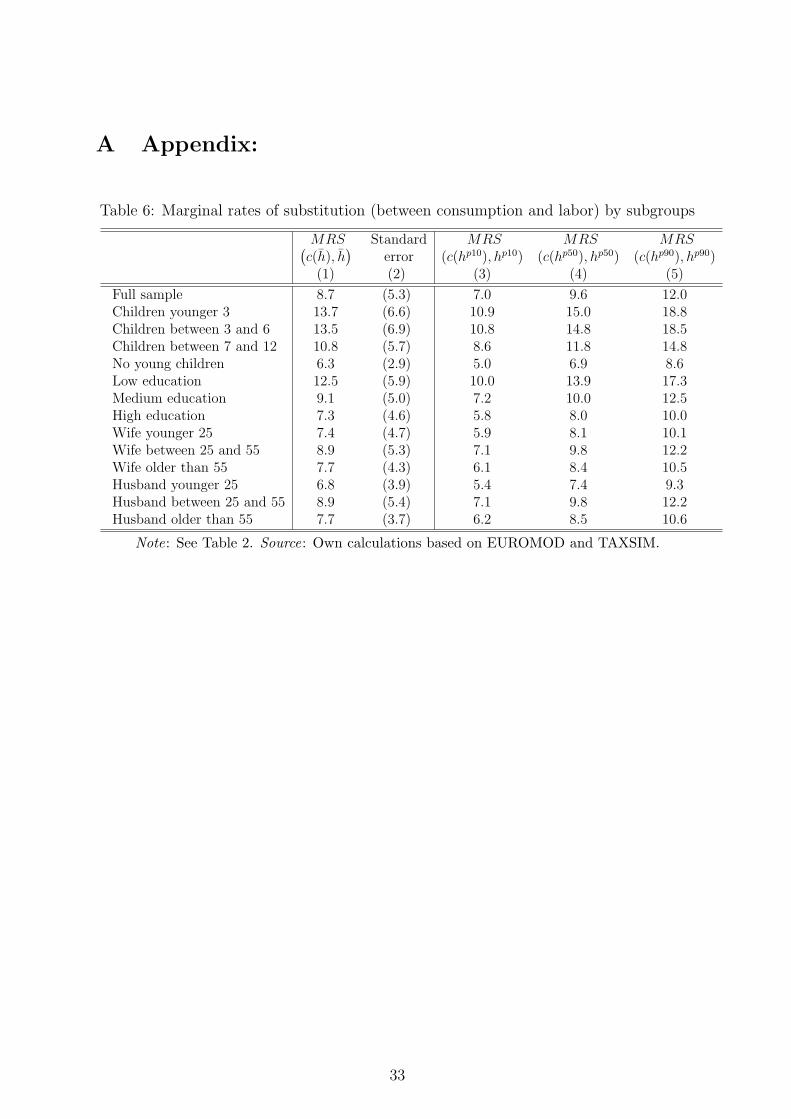
A Appendix:

Table 6: Marginal rates of substitution (between consumption and labor) by subgroups

MRS Standard MRS MRS MRS(c(h), h

)error (c(hp10), hp10) (c(hp50), hp50) (c(hp90), hp90)

(1) (2) (3) (4) (5)

Full sample 8.7 (5.3) 7.0 9.6 12.0Children younger 3 13.7 (6.6) 10.9 15.0 18.8Children between 3 and 6 13.5 (6.9) 10.8 14.8 18.5Children between 7 and 12 10.8 (5.7) 8.6 11.8 14.8No young children 6.3 (2.9) 5.0 6.9 8.6Low education 12.5 (5.9) 10.0 13.9 17.3Medium education 9.1 (5.0) 7.2 10.0 12.5High education 7.3 (4.6) 5.8 8.0 10.0Wife younger 25 7.4 (4.7) 5.9 8.1 10.1Wife between 25 and 55 8.9 (5.3) 7.1 9.8 12.2Wife older than 55 7.7 (4.3) 6.1 8.4 10.5Husband younger 25 6.8 (3.9) 5.4 7.4 9.3Husband between 25 and 55 8.9 (5.4) 7.1 9.8 12.2Husband older than 55 7.7 (3.7) 6.2 8.5 10.6

Note: See Table 2. Source: Own calculations based on EUROMOD and TAXSIM.

33

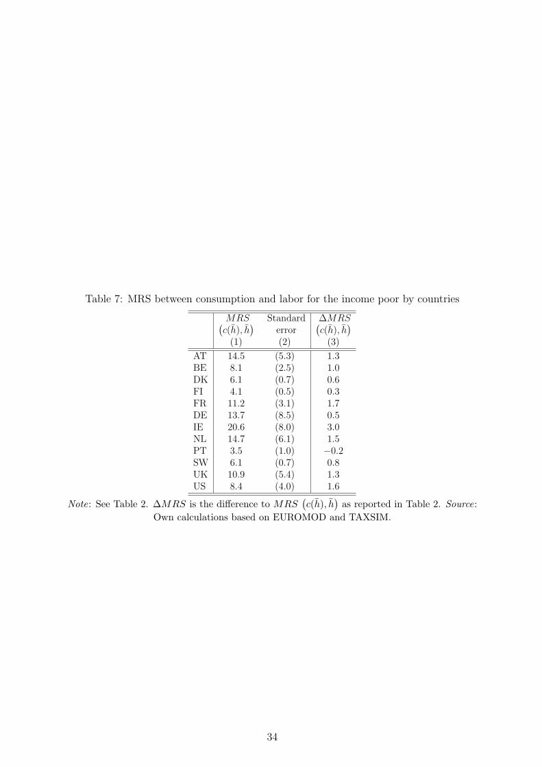
Table 7: MRS between consumption and labor for the income poor by countries

MRS Standard ∆MRS(c(h), h

)error

(c(h), h

)(1) (2) (3)

AT 14.5 (5.3) 1.3BE 8.1 (2.5) 1.0DK 6.1 (0.7) 0.6FI 4.1 (0.5) 0.3FR 11.2 (3.1) 1.7DE 13.7 (8.5) 0.5IE 20.6 (8.0) 3.0NL 14.7 (6.1) 1.5PT 3.5 (1.0) −0.2SW 6.1 (0.7) 0.8UK 10.9 (5.4) 1.3US 8.4 (4.0) 1.6

Note: See Table 2. ∆MRS is the difference to MRS(c(h), h

)as reported in Table 2. Source:

Own calculations based on EUROMOD and TAXSIM.

34

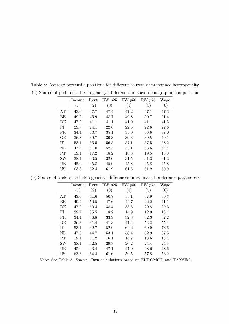
Table 8: Average percentile positions for different sources of preference heterogeneity

(a) Source of preference heterogeneity: differences in socio-demographic composition

Income Rent RW p25 RW p50 RW p75 Wage(1) (2) (3) (4) (5) (6)

AT 43.6 47.7 47.4 47.2 47.1 47.3BE 49.2 45.9 48.7 49.8 50.7 51.4DK 47.2 41.1 41.1 41.0 41.1 41.5FI 29.7 24.1 22.6 22.5 22.6 22.6FR 34.4 33.7 35.1 35.9 36.6 37.0GE 36.3 39.7 39.3 39.3 39.5 40.1IE 53.1 55.5 56.5 57.1 57.5 58.2NL 47.6 51.0 52.5 53.1 53.6 54.4PT 19.1 17.2 18.2 18.8 19.5 18.8SW 38.1 33.5 32.0 31.5 31.3 31.3UK 45.0 45.8 45.9 45.8 45.8 45.8US 63.3 62.4 61.9 61.6 61.2 60.9

(b) Source of preference heterogeneity: differences in estimated preference parameters

Income Rent RW p25 RW p50 RW p75 Wage(1) (2) (3) (4) (5) (6)

AT 43.6 41.6 50.7 55.1 57.9 59.3BE 49.2 50.5 47.6 44.7 42.2 41.1DK 47.2 50.4 38.4 33.3 29.8 29.3FI 29.7 35.5 18.2 14.9 12.9 13.4FR 34.4 36.8 33.9 32.8 32.3 32.2DE 36.3 31.4 41.3 47.4 52.2 55.4IE 53.1 42.7 52.9 62.2 69.9 78.6NL 47.6 44.7 53.1 58.4 62.9 67.5PT 19.1 21.2 16.1 14.7 13.6 13.4SW 38.1 42.5 29.3 26.2 24.4 24.5UK 45.0 43.4 47.1 47.9 48.6 48.6US 63.3 64.4 61.6 59.5 57.8 56.2

Note: See Table 3. Source: Own calculations based on EUROMOD and TAXSIM.

35

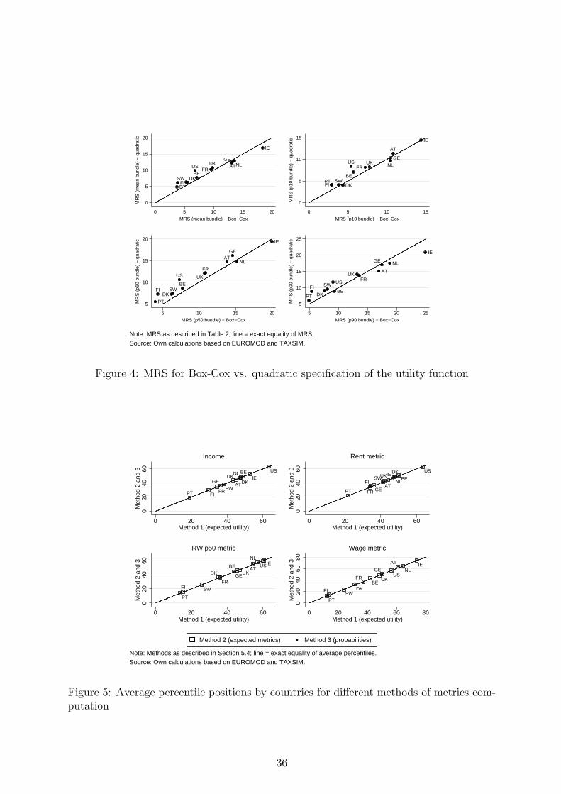
AT

BEDK

FI

FR

GE

IE

NL

PT

UK

SW

US

0

5

10

15

20M

RS

(m

ean

bund

le)

− q

uadr

atic

0 5 10 15 20MRS (mean bundle) − Box−Cox

AT

BE

DKFI

FR

GE

IE

NL

PT

UK

SW

US

0

5

10

15

MR

S (

p10

bund

le)

− q

uadr

atic

0 5 10 15MRS (p10 bundle) − Box−Cox

AT

BE

DKFI

FR

GE

IE

NL

PT

UK

SW

US

5

10

15

20

MR

S (

p50

bund

le)

− q

uadr

atic

5 10 15 20MRS (p50 bundle) − Box−Cox

AT

BEDK

FI

FR

GE

IE

NL

PT

UK

SW US

5

10

15

20

25

MR

S (

p90

bund

le)

− q

uadr

atic

5 10 15 20 25MRS (p90 bundle) − Box−Cox

Note: MRS as described in Table 2; line = exact equality of MRS.Source: Own calculations based on EUROMOD and TAXSIM.

Figure 4: MRS for Box-Cox vs. quadratic specification of the utility function

AT

BE

DK

FIFR

GEIE

NL

PT

UK

SW

US

020

4060

Met

hod

2 an

d 3

0 20 40 60Method 1 (expected utility)

Income

AT

BEDK

FI

FR GE

IE

NL

PT

UKSW

US

020

4060

Met

hod

2 an

d 3

0 20 40 60Method 1 (expected utility)

Rent metric

ATBEDK

FIFR

GE

IENL

PT

UK

SW

US

020

4060

Met

hod

2 an

d 3

0 20 40 60Method 1 (expected utility)

RW p50 metric

AT

BEDKFI

FR

GEIE

NL

PT

UK

SW

US

020

4060

80M

etho

d 2

and

3

0 20 40 60 80Method 1 (expected utility)

Wage metric

Note: Methods as described in Section 5.4; line = exact equality of average percentiles.Source: Own calculations based on EUROMOD and TAXSIM.

Method 2 (expected metrics) Method 3 (probabilities)

Figure 5: Average percentile positions by countries for different methods of metrics com-putation

36

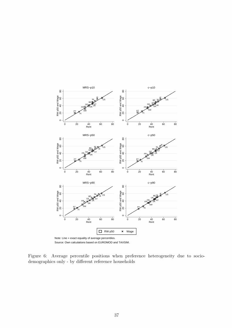
ATBE

DK

FI

FRGE

IENL

PT

UK

SW

US

020

4060

80R

W p

50 a

nd W

age

0 20 40 60 80Rent

MRS−p10

ATBE

DK

FI

FR

GE

IENL

PT

UK

SW

US

020

4060

80R

W p

50 a

nd W

age

0 20 40 60 80Rent

c−p10

AT

BE

DK

FI

FRGE

IENL

PT

UK

SW

US

020

4060

80R

W p

50 a

nd W

age

0 20 40 60 80Rent

MRS−p50

ATBE

DK

FI

FRGE

IENL

PT

UK

SW

US

020

4060

80R

W p

50 a

nd W

age

0 20 40 60 80Rent

c−p50

ATBE

DK

FI

FRGE

IENL

PT

UK

SW

US

020

4060

80R

W p

50 a

nd W

age

0 20 40 60 80Rent

MRS−p90

AT

BE

DK

FI

FRGE

IENL

PT

UK

SW

US

020

4060

80R

W p

50 a

nd W

age

0 20 40 60 80Rent

c−p90

Note: Line = exact equality of average percentiles.

Source: Own calculations based on EUROMOD and TAXSIM.

RW p50 Wage

Figure 6: Average percentile positions when preference heterogeneity due to socio-demographics only - by different reference households

37

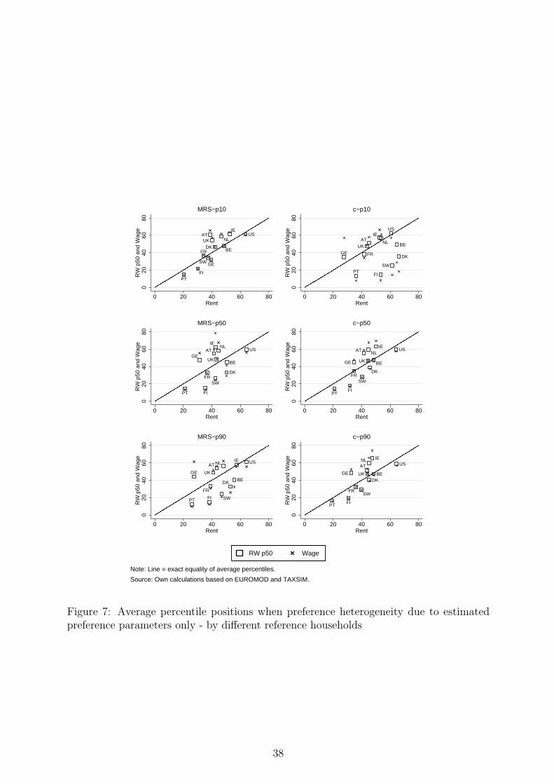
AT

BEDK

FI

FR

GE

IE

NL

PT

UK

SW

US

020

4060

80R

W p

50 a

nd W

age

0 20 40 60 80Rent

MRS−p10

ATBE

DK

FI

FRGE

IE

NL

PT

UK

SW

US

020

4060

80R

W p

50 a

nd W

age

0 20 40 60 80Rent

c−p10

AT

BE

DK

FI

FR

GE

IENL

PT

UK

SW

US

020

4060

80R

W p

50 a

nd W

age

0 20 40 60 80Rent

MRS−p50

AT

BE

DK

FI

FR

GE

IENL

PT

UK

SW

US

020

4060

80R

W p

50 a

nd W

age

0 20 40 60 80Rent

c−p50

AT

BEDK

FI

FR

GE

IENL

PT

UK

SW

US

020

4060

80R

W p

50 a

nd W

age

0 20 40 60 80Rent

MRS−p90

AT

BEDK

FI

FR

GE

IENL

PT

UK

SW

US

020

4060

80R

W p

50 a

nd W

age

0 20 40 60 80Rent

c−p90

Note: Line = exact equality of average percentiles.

Source: Own calculations based on EUROMOD and TAXSIM.

RW p50 Wage

Figure 7: Average percentile positions when preference heterogeneity due to estimatedpreference parameters only - by different reference households

38

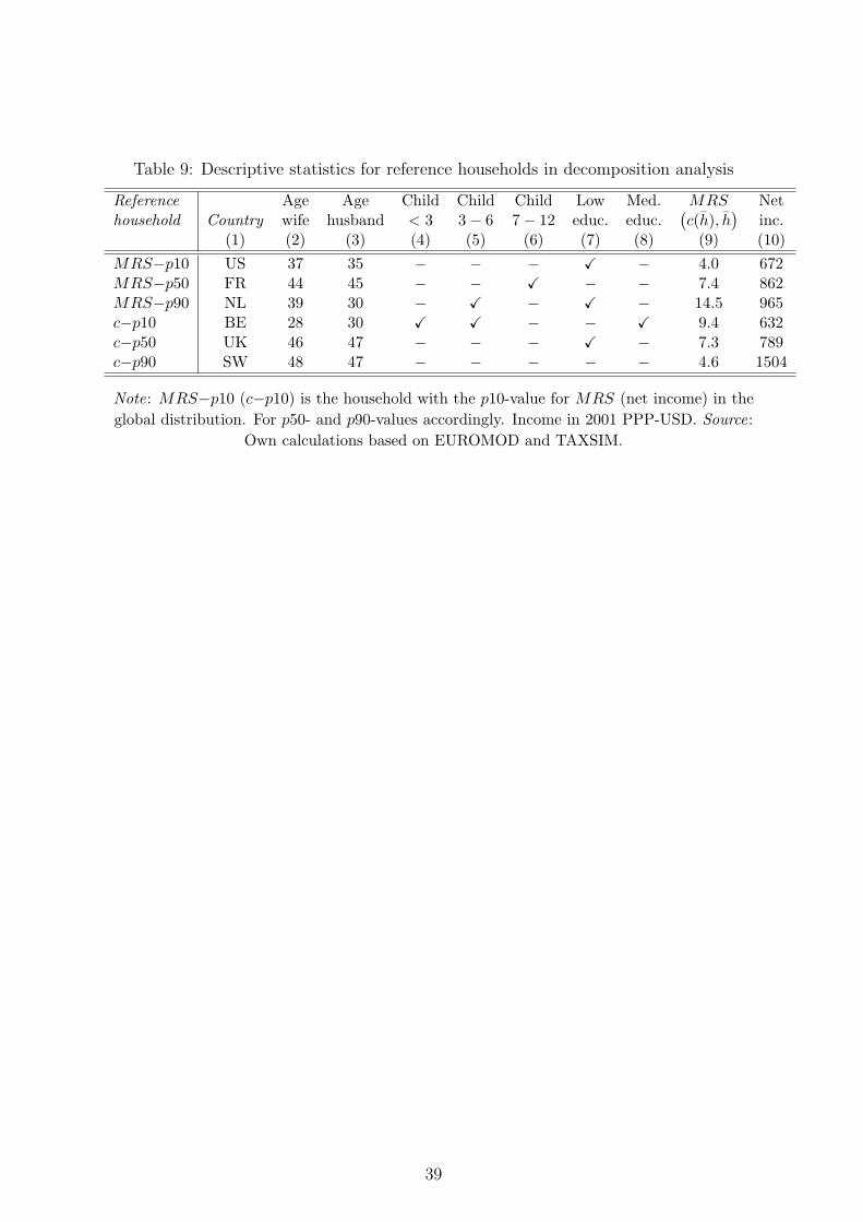
Table 9: Descriptive statistics for reference households in decomposition analysis

Reference Age Age Child Child Child Low Med. MRS Nethousehold Country wife husband < 3 3− 6 7− 12 educ. educ.

(c(h), h

)inc.

(1) (2) (3) (4) (5) (6) (7) (8) (9) (10)

MRS−p10 US 37 35 − − − X − 4.0 672MRS−p50 FR 44 45 − − X − − 7.4 862MRS−p90 NL 39 30 − X − X − 14.5 965c−p10 BE 28 30 X X − − X 9.4 632c−p50 UK 46 47 − − − X − 7.3 789c−p90 SW 48 47 − − − − − 4.6 1504

Note: MRS−p10 (c−p10) is the household with the p10-value for MRS (net income) in the

global distribution. For p50- and p90-values accordingly. Income in 2001 PPP-USD. Source:

Own calculations based on EUROMOD and TAXSIM.

39