Embed Size (px)
Citation preview
Heterogeneous Farmers’ Technology Adoption Decisions S. Jessica Zhu
Heterogeneous Farmers’
Technology Adoption Decisions:
Good on Average Is Not Good Enough∗
Jessica Zhu†
Job Market Paper
This Version: October 8, 2018
Latest Version: Click HERE
∗I am grateful to Laura Schechter for her invaluable advice and support. I also thank Emilia Tjernström,Jeremy Foltz, Zhidong Chen, Jared Hutchins, Ziqi Qiao, Charng-Jiun Yu, and seminar participants atUniversity of Wisconsin-Madison, University of Minnesota, Midwest International Economic DevelopmentConference (MIEDC), and AAEA Annual Meeting for helpful comments.†Department of Agricultural and Applied Economics, University of Wisconsin-Madison. Email:
[email protected]. Website: sjessicazhu.com.
1
Heterogeneous Farmers’ Technology Adoption Decisions S. Jessica Zhu
Abstract
In spite of the importance of agriculture sector and the persistently low agricultural
productivity, smallholders in Sub-Saharan Africa are unconcerned with the seemingly-
profitable modern technology - fertilizer, and at the same time are keen on the seemingly-
unbeneficial traditional technology - intercropping. This paper aims to solve that puzzle
and understand the rationale behind farmers’ decisions about agricultural technology
adoption. I construct a farmer’s decision-making model which takes into account both
the expected value and the variance of a farmer’s profit. Within this model, I build a
farmer’s production function that has three special properties: heterogeneous returns,
selection bias, and heterogeneous variances for each technology. Estimating this struc-
tural model with the Tanzania Living Standards Measurement Study panel dataset, I
discover that the expected returns of adopting the same technology vary significantly
across farmers. Furthermore, adopting fertilizer significantly increases expected yields
for farmers who adopt it every year, yet the higher expected returns are accompanied
by larger variances. On the other hand, adopting intercropping does not increase the
expected returns, but significantly decreases the variance of yields. Farmers’ technol-
ogy adoption decisions are influenced positively by the expected value of profits and
negatively by the variance of profits. These empirical results explain the low adoption
rates of an intensively promoted higher-average-return technology such as fertilizer, and
justify the high adoption rates of a seemingly-unprofitable technology such as intercrop-
ping.
Keywords: Technology adoption, heterogeneity in return, selection bias, risk aversion.
2
Heterogeneous Farmers’ Technology Adoption Decisions S. Jessica Zhu
1 Introduction
In Sub-Saharan African countries, the agriculture sector employs more than fifty percent
of the total labor force and provides on average fifteen percent of total GDP (OECD-FAO,
2016). Despite the importance of agriculture sector, farmers in these countries persistently
use traditional farming methods and face low agricultural productivity. Modern agricultural
technologies offer high expected returns on average and have been widely adopted in devel-
oped countries, but they have been seldom used in Sub-Saharan Africa. Numerous studies
have investigated and attempted to solve this conundrum. Various explanations are offered,
such as lacking information, missing input markets, and liquidity constraints, yet there is no
consensus on the justification. This paper aims to understand the rationale behind farm-
ers’ decisions about agricultural technology adoption. It examines a different hypothesis:
farmers’ decisions about adoption or non-adoption of modern technologies may be ratio-
nal responses to the return distributions they face. Expected returns and variances differ
across farmers and technologies. These differences could explain the variability in farmers’
technology adoptions.
Within the literature about agricultural technology adoption, a large collection of
studies focuses on the obstacles that have caused this insufficient usage, such as informa-
tion failure (Foster and Rosenzweig, 1995; Munshi, 2004; Conley and Udry, 2010), supply
shortages (Moser and Barrett, 2006), and credit constraints (Duflo et al., 2008). These stud-
ies implicitly assume that modern agricultural technologies are unambiguously better, and
therefore non-adoption must be the result of some failures - a market failure or an infor-
mation failure. While those factors contribute to the low and stagnating rate of technology
adoption, they cannot fully account for it. After decades of technology promotion and rapid
economic development, farmers have gained information on technologies and access to in-
puts. Yet, uptake of modern technologies remains low. One potential explanation for this is
that adoption of modern technology may not be optimal for everyone (Suri, 2011; Liu, 2013).
I examine this explanation and find results suggesting the assumption that low technology
3
Heterogeneous Farmers’ Technology Adoption Decisions S. Jessica Zhu
adoption is primarily driven by market failures may be incorrect.
This study contributes to the literature by constructing a model of farmer’s decision-
making which takes into account both the mean and the variance of a farmer’s profits.
Current literature about agricultural technology adoption is popularized with the expected
return models. However, in economies with limited insurance, the fluctuations in profits also
play crucial roles in farmers’ decisions. Both the expectation and the variability of profits
should be investigated. Furthermore, this paper borrows the concept of heterogeneity from
labor economics (Carneiro and Lee, 2004; Heckman and Li, 2004). The model allows the
effect on yield of adopting the same technology to be different across farmers and plots.
In addition, farmers are assumed to have knowledge of their own productivity for each
technology and choose which technology to adopt accordingly. Heterogeneous returns and
selection bias are equally relevant in the decisions about agricultural technology adoption,
but they have been understudied. This research attempts to fill in this gap, and relax the
common assumptions in the literature that farmers are both homogeneous and risk-neutral
expected value maximizers.
In my farmer’s decision-making model, I assume that farmers are expected utility
maximizers and may have preferences over both the mean and the variance of profits. At
the beginning of each farming season, farmers choose one agricultural technology set to
maximize their expected utility. They have four available choices: adopting nothing, adopt-
ing only inorganic fertilizer, adopting only intercropping, or adopting both fertilizer and
intercropping. The core of farmer’s decision making lays at farmer’s production, which is
substantially affected by his/her agricultural technology adoption choices. I construct the
farmer’s production function with three special properties: heterogeneous returns by farmer
and technology, selection bias by farmer, and heterogeneous variances by technology. An
important feature of my production model is that it allows farmers to consider multiple
technologies at once, rather than binary adoption decisions in isolation.
Empirically, I estimate this farmer’s decision-making model using the Tanzania Living
4
Heterogeneous Farmers’ Technology Adoption Decisions S. Jessica Zhu
Standards Measurement Study (LSMS) panel dataset. I first evaluate the farmer’s produc-
tion function using a correlated random coefficient (CRC) model. Next, I solve the intrinsic
characteristics of technology sets that affect the variance of productions through the feasible
generalized least squares (FGLS) method, and then I re-estimate the farmer’s production
function with weights. Lastly, I calculate farmers’ responses to both the expected value of
profit and the variance of profit (risk aversion level), and analyze the factors that influence
farmers’ agricultural technology adoption decisions.
My results show that expected returns to technology adoption vary across different
types of farmers and different technologies. Farmers are categorized into four groups based on
their adoption histories - never-adopter, dis-adopter, late-adopter, and always-adopter. For
farmers adopting only fertilizer and adopting both fertilizer and intercropping, the expected
returns in yields are significantly larger than zero for farmers who adopt it in every year,
aka always-adopters.1 The estimated expected returns of always-adopter are higher than
what a never-adopter would have achieved if he/she had adopted fertilizer or both tech-
nologies. This scenario indicates that farmers are rational, and many farmers do not adopt
fertilizer because it would not significantly increase their yields given their own and their
plot characteristics. In addition, the higher returns of adopting only fertilizer are accom-
panied by larger conditional variances of yields. On the other hand, compared to adopting
nothing, the additional expected return of adopting only intercropping is approximately zero
for every farmer. Nevertheless, adoption of intercropping leads to a significant reduction of
the conditional variance of yields. Furthermore, adopting both technologies is not a simple
summation of adopting only fertilizer and adopting only intercropping. This combination
represents a different technology. Using the solved distributions of profits, I demonstrate
that farmers respond positively to the expectation of profit and negatively to the variance
of profit when they make their technology adoption choices. Even after controlling for other
explanatory factors suggested in the literature on technology adoption, the influence of risk1In this paper, I define “yield” as dollar values of outputs per acre.
5
Heterogeneous Farmers’ Technology Adoption Decisions S. Jessica Zhu
is still important and significant in the farmer’s decision-making process. When predicting
farmer’s probability of adopting each technology, if I set the variances of technologies to be
zero, rather than their true values, the probability of adopting only fertilizer increases from
4% to 11%, while the probability of adopting only intercropping drops.
This paper designs and solves a structural model of farmer’s technology adoption de-
cision. This model is built to include five properties - heterogeneity in return, selection bias,
heterogeneity in variance, mean-variance expected utility and multiple technologies, which
are examined separately in the previous literature. The comprehensiveness of this model
provides a better representation of the reality. With a precise understanding of farmers’
rationale for agricultural technology adoption decisions, agricultural development policy-
makers could target their policy prescriptions from various perspectives that affect farmers’
expected utilities. For instance, policy-makers may reallocate spending away from less ef-
fective programs that spread more information about well-known technologies, and instead
focus on insurance programs to nudge capable farmers from their rational low-mean and
low-variance equilibrium to a better equilibrium, thereby improving farmer welfare.
2 Literature Review
This study is connected with three groups of literature: literature about agricultural technol-
ogy diffusion and adoption in development economics, literature about heterogeneous returns
to investment and self-selection behavior in labor economics, and literature about agricul-
tural production in agricultural economics. It contributes to current work by constructing
and solving a farmer’s decision-making model through combining knowledge from multiple
disciplines.
Reviewing the studies about technology adoption, the most renowned theme is about
information failure, which leads to various learning models as solutions. Foster and Rosen-
zweig (1995) and Munshi (2004) both examine the adoption rates of high-yielding seed vari-
6
Heterogeneous Farmers’ Technology Adoption Decisions S. Jessica Zhu
eties in the Indian Green Revolution. Foster and Rosenzweig (1995) find evidence for both
learning by doing and learning from others or social learning. Imperfect knowledge impedes
farmers’ adoption decisions. This dynamic improves as farmers accumulate experience, and
the increases of both farmers’ own experiences and neighbors’ experiences significantly raise
seed profitability and adoption. Munshi (2004) reaches a mixed result over different crops:
wheat growers learn from neighbors’ experiences, while rice growers benefit from own ex-
periences. Along the social interaction line, Conley and Udry (2010) study the adoption of
fertilizer for pineapple growing in Ghana, and suggest that there is social learning; farm-
ers modify their input uses to align with their informative neighbors. Bandiera and Rasul
(2006) investigate the adoption of sunflower in Mozambique, and find that farmers’ behaviors
are strongly correlated with their families’ and friends’ actions. The overarching takeaway
for this cluster of studies is that technology adoption rates are likely to be low due to the
lack of information. However, when farmers overcome information barriers, either from own
experience or social experience, adoption is boosted. While information and learning have
been the center of explanations for low adoption rates, these concepts become less influential
nowadays, thanks to decades of technology promotions. In this research, I choose to study
modern technologies which are well-known by farmers, so that information issue could be
avoided.
The next commonly studied factors that hinder technology adoption are input scarci-
ties, such as credit constraints and labor shortages. Moser and Barrett (2003) examine the
adoption of the System of Rice Intensification (SRI) in Madagascar, and attribute the low
adoption rate to additional labor requirements. When households have used their family
labor and hired labor to the full capacity, seasonal liquidity constraints may exist if the
modern technology requires extra labors. Croppenstedt et al. (2003) work on data about
Ethiopia and find that lacking financial resources to buy fertilizer is one of the main rea-
sons for non-adoption. Duflo et al. (2008) experiment with farmers in Western Kenya for
fertilizer purchases, and realize that an effective commitment device at harvest period could
7
Heterogeneous Farmers’ Technology Adoption Decisions S. Jessica Zhu
increase the technology adoption rate by 11 to 14 percentage points. To reflect on the factor
insufficiency issue, I select a couple technologies that require different inputs. Specifically,
one technology would demand additional labors, and the other technology would request
monetary resources.
Even though the adoption literature primarily focuses on reasons that have caused
low adoption rates, a new strand of works appears with the null hypothesis that farmers make
rational adoption decisions. Liu (2013) investigates the role of individual risk attitudes in the
adoption decision of Bt cotton. Through a field experiment in China, she finds that farmers
adopt the technology at different time because of their various risk preferences. Farmers
who overweight small probabilities are the first adopters of Bt cotton, and farmers who
have higher levels of risk aversion or loss aversion adopt Bt cotton later. Although the data
which I use for this study do not measure risk preference explicitly, I estimate it from my
expected utility function. Suri (2011) examines the heterogeneity in returns among farmers
and finds that adopting a new technology may lead to large returns on average, but offer
very low returns for marginal farmers. Using hybrid maize adoption data from Kenya, she
discovers that farmers’ decisions are rational - among the non-adopters, they either have
approximately zero gross returns or face high costs, while adopters are farmers who enjoy
positive returns and low costs.
In Suri (2011), she analyzes the impact of farmers’ comparative advantage on their
technology adoption and heterogeneous productions. While this approach is new to the agri-
culture setting, it has been more developed in the field of labor economics. For example,
when examining the effect of schooling on wages, economists observe people’s wages and
education levels, but do not know about people’s abilities and the reasons behind people’s
educational choices. Roy (1951) writes that individuals self-select into fishing or hunting,
based on their own abilities. Lemieux (1998) finds that because of their comparative ad-
vantage across sectors, workers make corresponding decisions about choosing union jobs vs.
non-union jobs. Card (1994) claims that there are heterogeneities in returns to education;
8
Heterogeneous Farmers’ Technology Adoption Decisions S. Jessica Zhu
individuals understand that difference, know about their own abilities, and make their school-
ing choices accordingly. Similarly, Carneiro and Lee (2004) and Heckman and Li (2004) show
that people self-select into college education, and the increase in lifetime earning due to col-
lege attendance is significantly higher for people who attend college than for people who do
not attend college. To parallel the logic into agricultural study, one observes the revenues of
farmers and their technology adoption decisions, but do not witnesses the rationale and the
causal effect behind it. This study builds a farmer’s production function with heterogeneous
returns and self-selection features, and aims to decipher that unobserved rationale.
Furthermore, as Chavas and Pope (1982) suggest that models of agricultural produc-
tion decisions under risks should always consider production uncertainty, I incorporate the
riskiness of technology in my farmer’s production function as the third feature. Pope and
Just (1977) and Just and Pope (1979) propose a general stochastic specification for produc-
tion function, so that the effects of input on output and the effects of input on variability of
output could be different. I employ their recommended function form to examine the impact
of technology use on risk. In addition to obtaining a variance component of the produc-
tion function, my model further allows farmers to respond to the variance characteristics of
technology in their expected utility functions, based on their risk attitude. Constructing a
model that include all relevant traits, which have been studied separately in previous works,
offers a more comprehensive and precise description of farmers’ actions, and provides the
instrument to investigate the reasoning behind farmers’ behaviors.
3 Theoretical Model
Consider a rural village in the developing world. At the beginning of each farming season,
farmers choose which agricultural technologies to adopt for each plot, among various existing
technologies.
9
Heterogeneous Farmers’ Technology Adoption Decisions S. Jessica Zhu
3.1 Agricultural Technology
To center the analysis on productivity and risk, I select the agricultural technologies following
two criteria. First, I choose technologies which have existed and been promoted in the
developing world for a significant amount of time, so that the information and learning
effect could be limited. Secondly, for considering the diversification of modern technologies,
I choose technologies which have different benefit distributions, i.e. mean and variance, and
require distinct inputs. Specifically, I select two agricultural technologies: inorganic fertilizer
(F ) and intercropping (I). The rationale of selecting those particular technologies lays at the
heterogeneity of farmers’ preferences and the heterogeneity of technologies’ characteristics.
According to the literature (Day, 1965; Fuller, 1965; Horowitz and Lichtenberg, 1993; Piepho,
1998), fertilizer has potential to increase productions significantly, yet the benefits come with
large production risks. On the other hand, intercropping is a technique which can reduce
the variance of productions and improve the soil quality over time (Horwith, 1985).
In this paper, I concentrate on those two technologies. Nevertheless, they could be
generalized to any technology. Also, regarding the benefit distribution of a specific technol-
ogy, I focus on its mean and variance. This assumption could be justified from two angles.
Either the profit function has a distribution which the knowledge of mean and variance are
enough to describe the whole distribution, such as normal distribution, gamma distribution,
and beta distribution; or farmers mainly care about those two perspectives of benefits, mean
and variance. Future researches could expand the benefit distribution to include skewness,
as farmers may have larger downside risk aversions.
3.2 Farmer’s Decision-Making Model
At the beginning of each farming season, farmers choose the agricultural technology set that
they want to adopt. Farmers could adopt nothing (N), only fertilizer (F ), only intercropping
(I), or both fertilizer and intercropping (B). Adopting both fertilizer and intercropping is
considered a separate technology itself, which allows for more flexibility in the complemen-
10
Heterogeneous Farmers’ Technology Adoption Decisions S. Jessica Zhu
tarity and substitutability of those two main technologies. From those four available choices,
D = {N, F, I, B}, farmers pick one to achieve their goal, i.e. maximizing the expected
utility. Let hD ={hN , hF , hI , hB
}be the adoption set containing 4 dummy variables (= 1
or = 0), which indicate farmers’ adoption decisions. After farmers decide the technology D,
the values of all hD are set. One, and only one, of those hD must equal 1 while the others
equal 0. For example, when farmers adopt only fertilizer, the model shows that hN = 0,
hF = 1, hI = 0, hB = 0; when farmers adopt both fertilizer and intercropping, the model
shows that hN = 0, hF = 0, hI = 0, hB = 1. Because each technology choice is exclusive to
others, the sum of four dummy variables is always one.
Assume farmers are expected utility maximizers. Their levels of expected utility are
affected by the production profit (π) - the expected profit (µ) and the variance of profit (v),
and the influences of those two factors are determined by the marginal utility of profit (m)
and the degree of risk aversion (ρ), as Equation 1:
maxhNijt,h
Fijt,h
Iijt,h
Bijt
EUijt = mµijt + ρvijt(1)
s.t. µijt = E[πijt]
vijt = E[(πijt)2]− (E[πijt])
2,
where i represents farmer, j refers to plot, and t stands for agriculture season.2 The choice
variables,{hNijt, h
Fijt, h
Iijt, h
Bijt
}, are factors of the production profits (π). The unit of analysis
is at the farmer-plot level (ij), due to the assumption that farmers make rational maximizing
decisions for each plot individually, rather than strategically allocate their resources across
all plots. If holding the belief that farmers enjoy high profits but suffer from a change of the
profit level (risk averse), I predict the directions of those two indices as m > 0 and ρ < 0.
The actual magnitudes and directions of those parameters are tested empirically.
Farmers’ production profits (π) are determined by the gross revenue (Y ) and the2The unique identifier of data is at household-plot level. I address it as farmer-plot level for an easier
interpretation of following analysis, with the belief that if a plot belongs to the same household over time,it is usually the same household member that plants it.
11
Heterogeneous Farmers’ Technology Adoption Decisions S. Jessica Zhu
farming cost (C),
(2) πijt = Yijt − Cijt.
Both the gross revenue and the farming cost are affected by the agricultural technology
adoption choices.
The total farming cost is a summation of two input costs - labor cost and fertilizer
cost,
(3) CDijt = labor costDijt + fertilizer costDijt.
The farming cost has a simple linear functional form and varies by the technology.
Assume the farmer’s production function has a Cobb-Douglas form. I define the
farmer’s production function of a plot under a particular technology set (D) as in Equation
4. Farmer’s revenues are affected by 3 components: 1) a technology-specific aggregate returns
to revenue, βD, which could be thought as a combination of the macroeconomic factors and
the characteristics of the agricultural technology set that affect the average revenues, 2) k
exogenous observable farming inputs (X), such as precipitation amounts and temperature
levels, 3) a technology-specific error (uD) , including time-invariant unobservable farmer
and technology characteristics, and time-varying random production shocks. Taking logs
of Equation 4, I get Equation 5, where yijt is the log of revenue, and other variables are
redefined to stand the logs of their corresponding variables.
Y Dijt = eβ
Dt (
k∏m=1
Xγmijtm)e(u
Dijt)(4)
yDijt = βDt + xijt′γ + uDijt,(5)
where xijt is a vector with dimension k× 1, γ is a vector of the output elasticity of farming
inputs. Assume the gross yield (Y ) follows a lognormal distribution, and thus the log of
yield (y) follows a normal distribution.
A point to note, in the current model set-up, I contribute both the extra quantity
of inputs required by a particular technology set and their associated input intensity effects
to the technology-specific aggregate returns component, counting those impacts as the tech-
nology attribute which affects the mean of revenues (βD); γ is not technology-specific. In
12
Heterogeneous Farmers’ Technology Adoption Decisions S. Jessica Zhu
addition, the yield variables are expressed as ratios of the land size, i.e. per acre. Farmers
would produce only when their expected profits are not negative.
For simplicity, I make two assumptions in this model. Firstly, there is no risk sharing
or strategical cooperation in the village. Farmers make their own decisions based on their
unique situations and are not influenced by their neighbors’ experience. Secondly, because
the farming inputs and crops choices are not the focus of this paper, I assume that once a
farmer chooses the technology he/she would like to use, the other inputs are predetermined.
For example, if he/she chooses intercropping, that implies a set amount of labor input. In
addition, the agricultural yields are presented as monetary values, so that the types of crops
are less relevant.3 The outcome variable could be perceived as one scalar, rather than a
vector of various crop productions.
3.3 Farmer’s Production Function
The core of farmers’ decision making lays at farmers’ productions; while farmers’ revenues are
substantially affected by their agricultural technology adoption choices. To study the impact
of technology adoption, I follow the methodology in labor economics and put additional
structure into the production function. When examining the effect of education on wages,
labor economists state two important issues needed to be considered: 1) returns to schooling
are heterogeneous in the population, 2) the unobservable ability in the residual term is
correlated with the regressor - schooling, as individuals know their abilities and choose their
education levels accordingly. Analogously, one could suspect that the effects of adopting
the same technology on revenues are different across farmers and plots. More importantly,
farmers may have good estimations of their productivity of each technology and choose the
adoption accordingly. In the following two sub-sections, I present these two properties in my
production function.3The influences of crop choices on technology adoptions are examined in the robustness checks section.
13
Heterogeneous Farmers’ Technology Adoption Decisions S. Jessica Zhu
3.3.1 Heterogeneity in Return
Equation 5 shows a farmer’s production function of adopting a specific technology set. In
each farming season, farmers could adopt any agricultural technology, the observed revenue
could be written as below,
yijt =∑D
hDijtyDijt(6)
= hFijt[βFt + xijtγ + uFijt] + hIijt[β
It + xijγ + uIijt]
+hBijt[βBt + xijtγ + uBijt] + (1− hFijt − hIijt − hBijt)[βNt + xijtγ + uNijt]
⇒ yijt = βNt + xijtγ + [(βFt − βNt ) + (uFijt − uNijt)]hFijt(7)
+[(βIt − βNt ) + (uIijt − uNijt)]hIijt + [(βBt − βNt ) + (uBijt − uNijt)]hBijt + uNijt.
Examining the three coefficients placed in front of the adoption dummies, [(βFt − βNt ) +
(uFijt− uNijt)], [(βIt − βNt ) + (uIijt− uNijt)], [(βBt − βNt ) + (uBijt− uNijt)], they represent the returns
to adopting only fertilizer, adopting only intercropping, and adopting both technologies,
respectively. Because all three coefficients include a uDijt − uNijt term, which varies at the
farmer-plot level (ij), the production function has the feature of heterogeneous return: re-
wards of each agricultural technology are farmer-plot-specific. Returns are random variables
with distributions. Estimating Equation 7 requires a random coefficient model.
3.3.2 Selection Bias in Adoption and Uncertainty of Production
To analyze the unobserved heterogeneity and the uncertainty of production deeper, I de-
compose the technology-specific error terms into two parts: productivity and shock. I put
additional structure on those two parts. For each farmer, he/she always has a general farm-
ing productivity (θij); if he/she adopts any technology, he/she also has a second productivity
component in term of that technology (θDij ). For the shock term, I assume that there is an
individual level idiosyncratic shock (ε), such as E(ε) = 0 and V (ε) = 1. More importantly,
the level of shock is amplified by a characteristic of the adopted technology (αD), which
captures the variability of yields across different technologies. This multiplicative setup of
14
Heterogeneous Farmers’ Technology Adoption Decisions S. Jessica Zhu
the shock term follows the concept of Just-Pope production function model (1977), to allow
distinct effects between the effect of technology on output and the effect of technology on
variability of output. The technology-specific production functions are modified as below:
yNijt = βNt + xijtγ + θij + (αN)12 εijt(8)
yFijt = βFt + xijtγ + θij + θFij + (αF )12 εijt(9)
yIijt = βIt + xijtγ + θij + θIij + (αI)12 εijt(10)
yBijt = βBt + xijtγ + θij + θBij + (αB)12 εijt.(11)
Rewritten the observed revenue using elaborated production functions,
yijt =∑D
hDijtyDijt(12)
= βNt + xijtγ + (βFt − βNt )hFijt + (βIt − βNt )hIijt + (βBt − βNt )hBijt
+θij + θFijhFijt + θIijh
Iijt + θBijh
Bijt + εijt{(αN)
12
+[(αF )12 − (αN)
12 ]hFijt + [(αI)
12 − (αN)
12 ]hIijt + [(αB)
12 − (αN)
12 ]hBijt}
= βNt + xijtγ + θij + [(βFt − βNt ) + θFij ]hFijt
+[(βIt − βNt ) + θIij]hIijt + [(βBt − βNt ) + θBij ]h
Bijt + εijt{(αN)
12
+[(αF )12 − (αN)
12 ]hFijt + [(αI)
12 − (αN)
12 ]hIijt + [(αB)
12 − (αN)
12 ]hBijt}.
Looking at the three coefficients placed in front of the adoption dummies again, (βFt −βNt )+
θFij , (βIt − βNt ) + θIij, (βBt − βNt ) + θBij , they are returns to technology adoption, including
an observed aggregate return term, and an unobserved productivity term. Because farmers’
adoption decisions (hDijt) and their expected profits (πijt) are tied together as in Equation 1,
and farmers’ productivity (θDij ) and their production outputs (yijt), thus their expected profits
(πijt), are correlated as in Equation 12, farmers’ productivity (θDij ) and farmers’ adoption
decisions (hDijt) are mutually related too. Given part of the coefficient on hDijt, parameter θDij ,
is correlated with the independent variable hDijt, the empirical analysis should be carried out
through a correlated random coefficient model with a control function.
15
Heterogeneous Farmers’ Technology Adoption Decisions S. Jessica Zhu
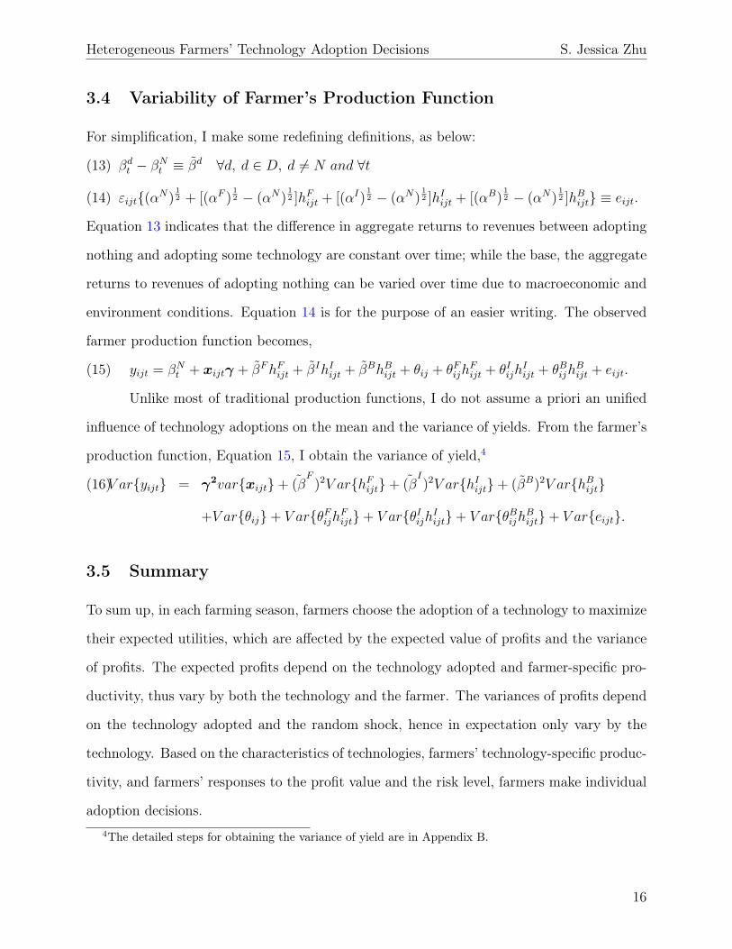
3.4 Variability of Farmer’s Production Function
For simplification, I make some redefining definitions, as below:
βdt − βNt ≡ βd ∀d, d ∈ D, d 6= N and ∀t(13)
εijt{(αN)12 + [(αF )
12 − (αN)
12 ]hFijt + [(αI)
12 − (αN)
12 ]hIijt + [(αB)
12 − (αN)
12 ]hBijt} ≡ eijt.(14)
Equation 13 indicates that the difference in aggregate returns to revenues between adopting
nothing and adopting some technology are constant over time; while the base, the aggregate
returns to revenues of adopting nothing can be varied over time due to macroeconomic and
environment conditions. Equation 14 is for the purpose of an easier writing. The observed
farmer production function becomes,
(15) yijt = βNt + xijtγ + βFhFijt + βIhIijt + βBhBijt + θij + θFijhFijt + θIijh
Iijt + θBijh
Bijt + eijt.
Unlike most of traditional production functions, I do not assume a priori an unified
influence of technology adoptions on the mean and the variance of yields. From the farmer’s
production function, Equation 15, I obtain the variance of yield,4
V ar{yijt} = γ2var{xijt}+ (βF
)2V ar{hFijt}+ (βI)2V ar{hIijt}+ (βB)2V ar{hBijt}(16)
+V ar{θij}+ V ar{θFijhFijt}+ V ar{θIijhIijt}+ V ar{θBijhBijt}+ V ar{eijt}.
3.5 Summary
To sum up, in each farming season, farmers choose the adoption of a technology to maximize
their expected utilities, which are affected by the expected value of profits and the variance
of profits. The expected profits depend on the technology adopted and farmer-specific pro-
ductivity, thus vary by both the technology and the farmer. The variances of profits depend
on the technology adopted and the random shock, hence in expectation only vary by the
technology. Based on the characteristics of technologies, farmers’ technology-specific produc-
tivity, and farmers’ responses to the profit value and the risk level, farmers make individual
adoption decisions.4The detailed steps for obtaining the variance of yield are in Appendix B.
16
Heterogeneous Farmers’ Technology Adoption Decisions S. Jessica Zhu
4 Data
The dataset employed by this research is the Tanzania National Panel Survey (TZNPS),
which is part of the World Bank Living Standards Measurement Study (LSMS). It is a
nationally-representative integrated household survey. It is repeated biennially and has four
waves: 2008-2009, 2010-2011, 2012-2013, and 2014-2015. In this paper, I use the middle two
waves of data, 2010-2011 round and 2012-2013 round, since they use more similar question-
naires and have more overlapping samples. The Tanzania National Panel Survey covers a
broad range of topics. The main subjects I concentrated on are its extensive information of
households’ farming practices and demographic characteristics.
4.1 Household and Plot Characteristics
The TZNPS sampled 26 regions out of 31 regions of Tanzania, aiming to be representative
for the whole country. In round 1 (2008-2009), it surveyed 125 districts, 337 enumeration ar-
eas/villages, 3265 households, and 5152 plots. In the following rounds, all original households
were revisited and re-interviewed. If any adult members have moved to other locations, they
were all tracked and re-interviewed at current locations with their new households. Because
of the splitting off, in round 2 (2010-2011), the survey contained 129 districts, 368 enumer-
ation areas/villages, 3924 households, and 6038 plots; in round 3 (2012-2013), the survey
covered 132 districts, 384 enumeration areas/villages, 5010 households, and 7457 plots.5 In
all later (non-first) rounds of data, the surveys included unique household and plot identifiers
of both the current round and the previous round. Thus, if the household or the plot have
been interviewed before, I could match them across data rounds.
For all data analysis, I use a balanced panel constructed from round 2 and round
3 data. The reason for a balanced panel is that estimating my structural model requires
knowing farmers’ adoption choices of all years. In each year, about 80% of plots were5The data expansion across rounds is relative huge comparing to other studies; but this pattern is verified
both by the survey documents and the dataset.
17
Heterogeneous Farmers’ Technology Adoption Decisions S. Jessica Zhu
cultivated, 10-15% of plots were fallow, and the rest of plots were rented out, given out, forest,
or in other use. Moreover, among the cultivated plots, 5% of plots were not harvested due
to destruction (3%), still growing in plot (1%), and other reasons (1%), when the interviews
were conducted. Limiting the sample to plots that have been cultivated and harvested in
both rounds, there are 1638 households and 2539 plots.6 I further restrict the sample to
observations with non-missing values for all variables used in the analysis, and end up with
1628 households and 2523 plots, aka the analysis sample.
Table 1 presents the descriptive statistics of sampled households. Around 87% of
households located at rural area, yet some urban households cultivated plots in the long
rainy season as well. Most of households had male heads, about 77%. Roughly 85% of
household heads had the main occupation in agriculture, while other household members
could be in charge of the household farming too. The average family size was 5.8, including
3.3 active members (age 12-60) and 2.5 dependents (children and elders). The average annual
temperature was about 22.6◦C; and the average annual rainfall in the past 12 months was
round 800mm.
Table 2 describes the characteristics of plots. On average, plots were 2.9 acres, had
above average soil quality where 1 stands for bad quality and 3 stands for good quality, and
medium steepness where 1 stands for flat and 3 stands for very steep. Very few plots (4%)
had been fallowed before7; while approximately 75% of plots could be sold by their belonging
households. Each plot usually used 64 days per acre of family labor, with helps from hired
labors that were worth 6 dollar per acre. Also, around 1 dollar worth of pesticides were
applied on the plot. Lastly, the harvest amounts were about 124 dollars per acre.8
6The sample size has dropped significantly because in each year, different plots got fallow and happenedto be not harvested. The accumulation of rotated 24% (= 1− 80%× 95%) has resulted a large amount.
7This low rate could be due to my selection of plots that were not fallowed in both farming season2010-2011 and farming season 2012-2013.
8These harvest values are farmers’ self-reported estimated values of their harvests. Given that farmersmay have different perceptions for crop prices, later I will create another harvest value variable using reportedharvest quantities (kg), and village prices and/or district prices as robustness checks.
18
Heterogeneous Farmers’ Technology Adoption Decisions S. Jessica Zhu
4.2 Farming Practices
Table 3, a transition matrix of farmers’ adoptions, shows descriptive statistics of farmers’
adoption of the four exclusive agricultural technology mentioned in Section 3.2, at the farmer-
plot level. Across the two farming seasons, the percentages of technology adoptions at farmer-
plot level were stable. There were approximately 37.6%-39.5% of plots adopted neither
technology, 7.8%-8.0% of plots adopted only fertilizer, 44.1%-45.6% of plots adopted only
intercropping, and 8.6%-8.8% of plots adopted both technologies. Nevertheless, if reading
the diagonal of Table 3, one could see that only 58.5% of plots adopted the same technology
across two years, and the other half of plots experienced different technologies over time. The
technology switching behaviors of farmers are essential for the structural model estimation,
i.e. creating the counterfactual.
5 Empirical Strategy
To empirically study farmers’ decisions about agricultural technology adoption, I estimate
the farmer’s decision-making model through four parts. In the first step, I evaluate the
farmer’s production function as a correlated random coefficient (CRC) model, and substi-
tute farmer’s unobservable and endogenous productivity with its linear projection on the
farmer’s full history of adoptions and their interactions. In the second step, I decompose
the previously estimated residual term of farmer’s production function through the feasible
generalized least squares (FGLS) method. Thus, I separate out the intrinsic characteristic of
technology set that affects the variance of productions. Then, I re-estimate the production
function with a weight derived from the previous step, thus all coefficients are updated to
be both consistent and asymptotic efficient. Lastly, I bring the estimated production values
back into the farmer’s expected utility function. Using the alternative-specific conditional
logit method, I calculate farmers’ responses to the expected value of profit and the variance
of profit, and analyze factors that influence farmers’ technology adoption decisions.
19
Heterogeneous Farmers’ Technology Adoption Decisions S. Jessica Zhu
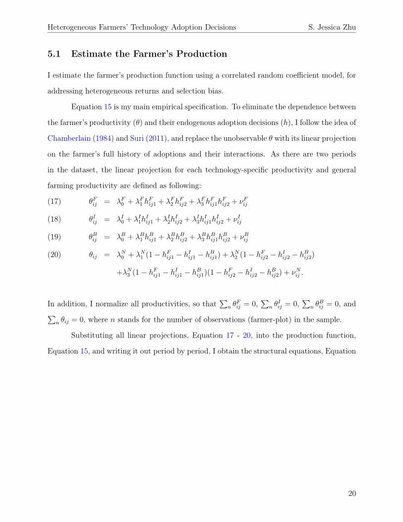
5.1 Estimate the Farmer’s Production
I estimate the farmer’s production function using a correlated random coefficient model, for
addressing heterogeneous returns and selection bias.
Equation 15 is my main empirical specification. To eliminate the dependence between
the farmer’s productivity (θ) and their endogenous adoption decisions (h), I follow the idea of
Chamberlain (1984) and Suri (2011), and replace the unobservable θ with its linear projection
on the farmer’s full history of adoptions and their interactions. As there are two periods
in the dataset, the linear projection for each technology-specific productivity and general
farming productivity are defined as following:
θFij = λF0 + λF1 hFij1 + λF2 h
Fij2 + λF3 h
Fij1h
Fij2 + νFij(17)
θIij = λI0 + λI1hIij1 + λI2h
Iij2 + λI3h
Iij1h
Iij2 + νIij(18)
θBij = λB0 + λB1 hBij1 + λB2 h
Bij2 + λB3 h
Bij1h
Bij2 + νBij(19)
θij = λN0 + λN1 (1− hFij1 − hIij1 − hBij1) + λN2 (1− hFij2 − hIij2 − hBij2)(20)
+λN3 (1− hFij1 − hIij1 − hBij1)(1− hFij2 − hIij2 − hBij2) + νNij .
In addition, I normalize all productivities, so that∑
n θFij = 0,
∑n θ
Iij = 0,
∑n θ
Bij = 0, and∑
n θij = 0, where n stands for the number of observations (farmer-plot) in the sample.
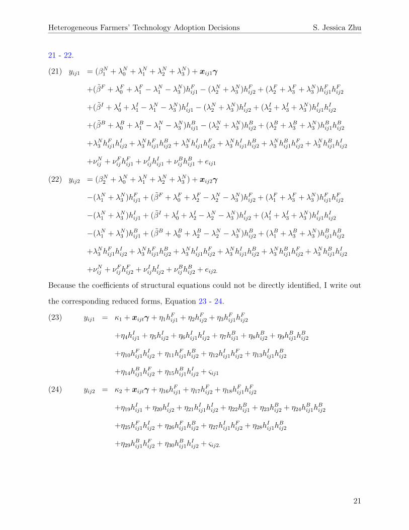
Substituting all linear projections, Equation 17 - 20, into the production function,
Equation 15, and writing it out period by period, I obtain the structural equations, Equation
20
Heterogeneous Farmers’ Technology Adoption Decisions S. Jessica Zhu
21 - 22.
yij1 = (βN1 + λN0 + λN1 + λN2 + λN3 ) + xij1γ(21)
+(βF + λF0 + λF1 − λN1 − λN3 )hFij1 − (λN2 + λN3 )hFij2 + (λF2 + λF3 + λN3 )hFij1hFij2
+(βI + λI0 + λI1 − λN1 − λN3 )hIij1 − (λN2 + λN3 )hIij2 + (λI2 + λI3 + λN3 )hIij1hIij2
+(βB + λB0 + λB1 − λN1 − λN3 )hBij1 − (λN2 + λN3 )hBij2 + (λB2 + λB3 + λN3 )hBij1hBij2
+λN3 hFij1h
Iij2 + λN3 h
Fij1h
Bij2 + λN3 h
Iij1h
Fij2 + λN3 h
Iij1h
Bij2 + λN3 h
Bij1h
Fij2 + λN3 h
Bij1h
Iij2
+νNij + νFijhFij1 + νIijh
Iij1 + νBijh
Bij1 + eij1
yij2 = (βN2 + λN0 + λN1 + λN2 + λN3 ) + xij2γ(22)
−(λN1 + λN3 )hFij1 + (βF + λF0 + λF2 − λN2 − λN3 )hFij2 + (λF1 + λF3 + λN3 )hFij1hFij2
−(λN1 + λN3 )hIij1 + (βI + λI0 + λI2 − λN2 − λN3 )hIij2 + (λI1 + λI3 + λN3 )hIij1hIij2
−(λN1 + λN3 )hBij1 + (βB + λB0 + λB2 − λN2 − λN3 )hBij2 + (λB1 + λB3 + λN3 )hBij1hBij2
+λN3 hFij1h
Iij2 + λN3 h
Fij1h
Bij2 + λN3 h
Iij1h
Fij2 + λN3 h
Iij1h
Bij2 + λN3 h
Bij1h
Fij2 + λN3 h
Bij1h
Iij2
+νNij + νFijhFij2 + νIijh
Iij2 + νBijh
Bij2 + eij2.
Because the coefficients of structural equations could not be directly identified, I write out
the corresponding reduced forms, Equation 23 - 24.
yij1 = κ1 + xijtγ + η1hFij1 + η2h
Fij2 + η3h
Fij1h
Fij2(23)
+η4hIij1 + η5h
Iij2 + η6h
Iij1h
Iij2 + η7h
Bij1 + η8h
Bij2 + η9h
Bij1h
Bij2
+η10hFij1h
Iij2 + η11h
Fij1h
Bij2 + η12h
Iij1h
Fij2 + η13h
Iij1h
Bij2
+η14hBij1h
Fij2 + η15h
Bij1h
Iij2 + ςij1
yij2 = κ2 + xijtγ + η16hFij1 + η17h
Fij2 + η18h
Fij1h
Fij2(24)
+η19hIij1 + η20h
Iij2 + η21h
Iij1h
Iij2 + η22h
Bij1 + η23h
Bij2 + η24h
Bij1h
Bij2
+η25hFij1h
Iij2 + η26h
Fij1h
Bij2 + η27h
Iij1h
Fij2 + η28h
Iij1h
Bij2
+η29hBij1h
Fij2 + η30h
Bij1h
Iij2 + ςij2.
21
Heterogeneous Farmers’ Technology Adoption Decisions S. Jessica Zhu
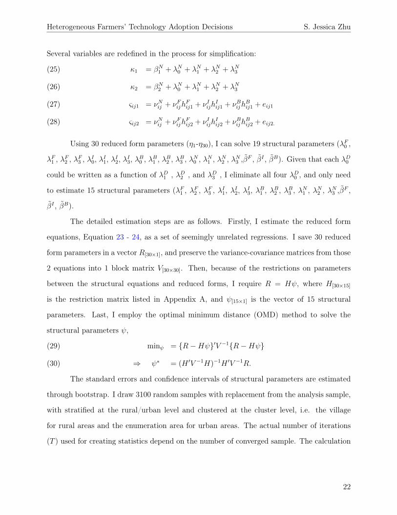
Several variables are redefined in the process for simplification:
κ1 = βN1 + λN0 + λN1 + λN2 + λN3(25)
κ2 = βN2 + λN0 + λN1 + λN2 + λN3(26)
ςij1 = νNij + νFijhFij1 + νIijh
Iij1 + νBijh
Bij1 + eij1(27)
ςij2 = νNij + νFijhFij2 + νIijh
Iij2 + νBijh
Bij2 + eij2.(28)
Using 30 reduced form parameters (η1-η30), I can solve 19 structural parameters (λF0 ,
λF1 , λF2 , λF3 , λI0, λI1, λI2, λI3, λB0 , λB1 , λB2 , λB3 , λN0 , λN1 , λN2 , λN3 ,βF , βI , βB). Given that each λD0
could be written as a function of λD1 , λD2 , and λD3 , I eliminate all four λD0 , and only need
to estimate 15 structural parameters (λF1 , λF2 , λF3 , λI1, λI2, λI3, λB1 , λB2 , λB3 , λN1 , λN2 , λN3 ,βF ,
βI , βB).
The detailed estimation steps are as follows. Firstly, I estimate the reduced form
equations, Equation 23 - 24, as a set of seemingly unrelated regressions. I save 30 reduced
form parameters in a vector R[30×1], and preserve the variance-covariance matrices from those
2 equations into 1 block matrix V[30×30]. Then, because of the restrictions on parameters
between the structural equations and reduced forms, I require R = Hψ, where H[30×15]
is the restriction matrix listed in Appendix A, and ψ[15×1] is the vector of 15 structural
parameters. Last, I employ the optimal minimum distance (OMD) method to solve the
structural parameters ψ,
minψ = {R−Hψ}′V −1{R−Hψ}(29)
⇒ ψ∗ = (H ′V −1H)−1H ′V −1R.(30)
The standard errors and confidence intervals of structural parameters are estimated
through bootstrap. I draw 3100 random samples with replacement from the analysis sample,
with stratified at the rural/urban level and clustered at the cluster level, i.e. the village
for rural areas and the enumeration area for urban areas. The actual number of iterations
(T ) used for creating statistics depend on the number of converged sample. The calculation
22
Heterogeneous Farmers’ Technology Adoption Decisions S. Jessica Zhu
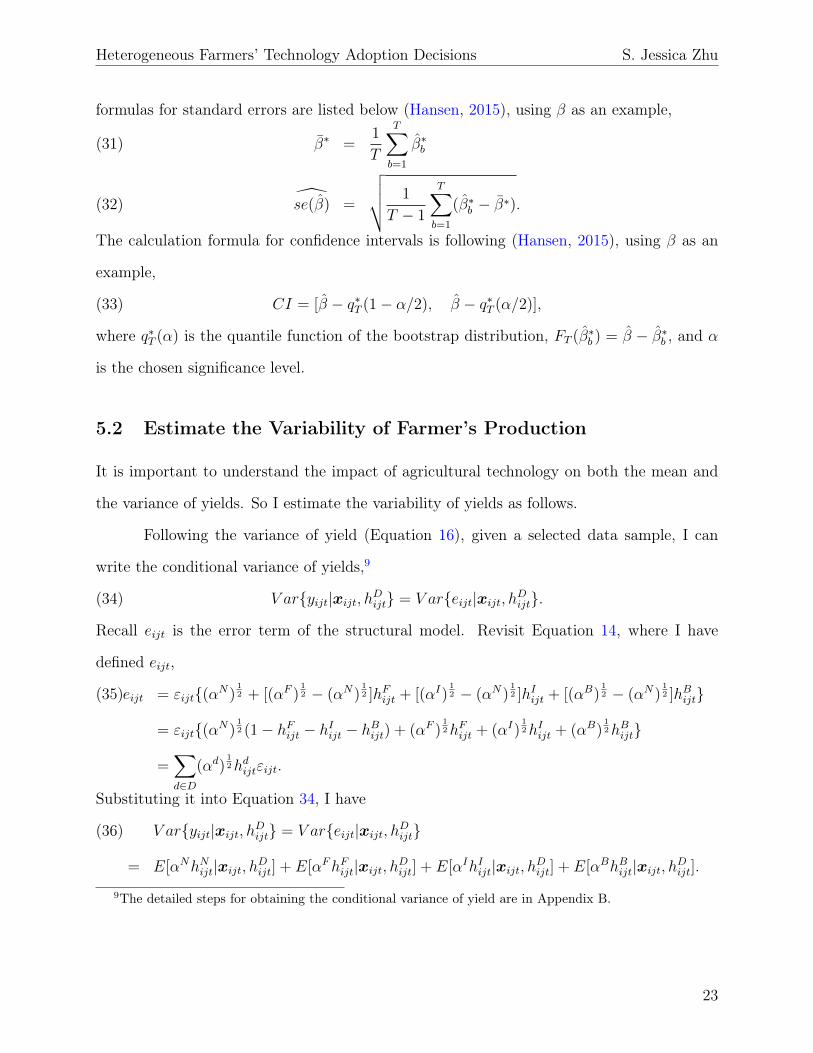
formulas for standard errors are listed below (Hansen, 2015), using β as an example,
β∗ =1
T
T∑b=1
β∗b(31)
se(β) =
√√√√ 1
T − 1
T∑b=1
(β∗b − β∗).(32)
The calculation formula for confidence intervals is following (Hansen, 2015), using β as an
example,
(33) CI = [β − q∗T (1− α/2), β − q∗T (α/2)],
where q∗T (α) is the quantile function of the bootstrap distribution, FT (β∗b ) = β − β∗b , and α
is the chosen significance level.
5.2 Estimate the Variability of Farmer’s Production
It is important to understand the impact of agricultural technology on both the mean and
the variance of yields. So I estimate the variability of yields as follows.
Following the variance of yield (Equation 16), given a selected data sample, I can
write the conditional variance of yields,9
(34) V ar{yijt|xijt, hDijt} = V ar{eijt|xijt, hDijt}.
Recall eijt is the error term of the structural model. Revisit Equation 14, where I have
defined eijt,
eijt = εijt{(αN)12 + [(αF )
12 − (αN)
12 ]hFijt + [(αI)
12 − (αN)
12 ]hIijt + [(αB)
12 − (αN)
12 ]hBijt}(35)
= εijt{(αN)12 (1− hFijt − hIijt − hBijt) + (αF )
12hFijt + (αI)
12hIijt + (αB)
12hBijt}
=∑d∈D
(αd)12hdijtεijt.
Substituting it into Equation 34, I have
V ar{yijt|xijt, hDijt} = V ar{eijt|xijt, hDijt}(36)
= E[αNhNijt|xijt, hDijt] + E[αFhFijt|xijt, hDijt] + E[αIhIijt|xijt, hDijt] + E[αBhBijt|xijt, hDijt].9The detailed steps for obtaining the conditional variance of yield are in Appendix B.
23
Heterogeneous Farmers’ Technology Adoption Decisions S. Jessica Zhu
In addition, by the definition of variance, I know,
(37) V ar{eijt|xijt, hDijt} = E[e2ijt|xijt, hDijt]− E[eijt|xijt, hDijt]2 = E[e2ijt|xijt, hDijt].
Combining Equation 36 and Equation 37 together,
V ar{yijt|xijt, hDijt} = V ar{eijt|xijt, hDijt}(38)
= E[e2ijt|xijt, hDijt]
= E[αNhNijt|xijt, hDijt] + E[αFhFijt|xijt, hDijt] + E[αIhIijt|xijt, hDijt] + E[αBhBijt|xijt, hDijt].
From this equation, one could see that the conditional variance of yield is clearly affected by
the individual technology choice. It indicates a case of heteroskedasticity.
To examine the impact of the variance characteristic (αD) of adopted technology (hDijt)
on the variability of yields, I adopt the feasible generalized least squares (FGLS) estimation
method. Assume the conditional variance of yield has an exponential function form, to
guarantee positive values for estimated variances,
V ar(yijt|xijt, hDijt) = exp{αNhNijt + αFhFijt + αIhIijt + αBhBijt + uijt}.(39)
Because coefficients from the first-step estimating the production function are consistent,
e2ijt is a consistent estimator of e2ijt. I can estimate the variance function with an ordinary
least squares regression as following,
e2ijt = exp{αNhNijt + αFhFijt + αIhIijt + αBhBijt + uijt}(40)
⇒ log(e2ijt) = αNhNijt + αFhFijt + αIhIijt + αBhBijt + uijt,(41)
where eijt is the residual term from the first step estimation and log(e2ijt) is calculated. For
an easier interpretation of the technology effects, I also estimate an equivalent equation,
log(e2ijt) = ι0 + αFhFijt + αIhIijt + αBhBijt + uijt.(42)
The coefficients placed in front of adoption dummy variables, αF , αI , αB, represent the
impacts of adopting technologies - fertilizer, intercropping, and both technologies - on the
variances of farmers’ yields, respectively, in addition to the impact of adopting nothing.
One could perceive those impacts as intrinsic characteristics of those technologies. Some
technologies lead to a larger variation in the yields, while others reduce that variability.
24
Heterogeneous Farmers’ Technology Adoption Decisions S. Jessica Zhu
5.3 Re-Estimate the Farmer’s Production
Because of the heteroskedasticity which is demonstrated in the second step, coefficients of
the production function acquired through the CRC model in the first step are unbiased and
consistent, but inefficient. To correct the heteroskedasticity, I re-estimate the production
function with a weight. The weight is the estimated conditional standard deviation of yield,
i.e. the square root of the exponential of the fitted value, ωijt =√efitted value =
√e
log( ˆeijt2).
The updated estimators of structural parameters are now unbiased, consistent, and asymp-
totically efficient.
5.4 Estimate Farmer’s Expected Utility
After fully solved the log version of production function, I progress to the underlying structure
of farmers’ technology adoption decisions.
To estimate the farmer’s expected utility function, several additional calculations are
required. From the previous three steps, I have derived the conditional expected value and
the conditional variance of log of yield through computing the linear predictions after the
regression analysis. The specific values are calculated as below. The first groups of equations
list the conditional expected values of log of yields under each technology adoption scenario:
E[ ˆyNijt|xijt, hNijt = 1] = βNt + xijtγ + θij(43)
E[ ˆyFijt|xijt, hFijt = 1] = βFt + xijtγ + θij + θFij(44)
E[ ˆyIijt|xijt, hIijt = 1] = βIt + xijtγ + θij + θIij(45)
E[ ˆyBijt|xijt, hBijt = 1] = βBt + xijtγ + θij + θBij .(46)
Next groups of equations list the conditional variance of log of yields under each technology
25
Heterogeneous Farmers’ Technology Adoption Decisions S. Jessica Zhu
adoption scenario:
V ar[ ˆyNijt|xijt, hNijt = 1] = elog(e2ijt) = ea
N(47)
V ar[ ˆyFijt|xijt, hFijt = 1] = elog(e2ijt) = ea
F(48)
V ar[ ˆyIijt|xijt, hIijt = 1] = elog(e2ijt) = ea
I(49)
V ar[ ˆyBijt|xijt, hBijt = 1] = elog(e2ijt) = ea
B.(50)
The conditional expected values of log of yields vary by both the technology and the
farmer-plot, while the conditional variance of log of yields only differ by the technology.
Yet, the variables needed in the expected utility function are the conditional expected
value and the conditional variance of yield. With the assumption that the yield follows a
lognormal distribution, I translate those values of log of yield to values of yield through the
distribution formula. Because y ∼ N (E[y], V ar[y]) and Y = ey, I have E(Y ) = eE[y]+0.5V ar[y],
and V ar(Y ) = [eV ar[y] − 1] × [e2E[y]+V ar[y]]. As a result, for each farmer-plot, I have 4
conditional expected values of yield and 4 conditional variance of yield, corresponding to
each technology adoption case.
In addition, recall the farming cost is defined as a summation of the labor cost and
the fertilizer cost, CDijt = laborcostDijt+fertilizercost
Dijt. All costs are calculated as dollar per
acre. The labor costs include both the family labor values and the hired labor values.10 For
each technology, I calculate the average labor costs and fertilizer costs among farmers who
adopted that technology in a village (rural) / an enumeration area (urban), and then apply
those average costs to all farmers in that specific village/enumeration area. As a result, the
farming costs vary by the technology choice, the location, and the farming season. For each
farmer-plot, I have 4 estimated farming costs, one for each technology adoption case.
Following the definition of profit as in Equation 2 and given that the farming cost is10The family labor values are computed through multiplying the adjusted total family labor days with
the adjusted labor day wage. The adjusted total family labor days are the half of self-reported total familylabor days. According to Arthia et al. (2018), at the plot level, the family labor usages reported in theTZNPS through the recall-survey method were about 1.83 times higher than the “true” labor usages, whichwere collected through weekly visits. The adjusted labor day wage are estimated using the subsistenceagricultural worker’s day wage and the hired labor’s day wage and then devalued by 50% (Deutschmannet al., 2018). The hired labor costs and the fertilizer costs are directly reported in the TZNPS.
26
Heterogeneous Farmers’ Technology Adoption Decisions S. Jessica Zhu
a scalar, I obtain the expected value of profit and the variance of profit,
µDijt = E[Y Dijt|xijt, hDijt]− CD
ijt(51)
vDijt = V ar[Y Dijt|xijt, hDijt].(52)
With these two main variables in hand, I begin to decipher the rationale of farmers’ agri-
cultural technology adoption decisions. I use the alternative-specific conditional logit model
(ASC logit), aka the McFadden’s choice model, to study the factors which influence the
farmer’s decision-making. In each farming season, farmers face 4 alternative technology
choices. Under the assumption that farmers are rational expected utility maximizer, they
would choose the technology which gives them the highest expected utility. Employing
farmers’ actual adoption decisions, I solve the impacts of potential factors.
Starting with a basic model as Equation 1,
(53) maxhNijt,h
Fijt,h
Iijt,h
Bijt
EUijt = mµijt + ρvijt,
where the expected value of profits and the variance of profits for each technology adoption
scenario are the alternative-specific variables, and the year fixed effect is the case-specific
variable, i.e. farmer-plot-specific variable. I derive farmers’ responses to the profit value (m)
and the variance of profit (ρ), both the magnitude and the direction.
Furthermore, since existing works have offered different explanations for farmers’
adoption decisions, I enhance my basic decision-making model. I include 4 additional groups
of potential influencing factors, which have been shown in the literature,
(54) maxhNijt,h
Fijt,h
Iijt,h
Bijt
EUijt = mµijt + ρvijt + φTZTijt + φLZL
ijt + φMZMijt + φCZC
ijt,
where ZTijt represents a group of distance variables which aim to capture the potential
difficulty of traveling to the market, ZLijt represents a group of family composition variables
which aim to capture the potential labor constraint, ZMijt represents a group of family financial
situation variables which aim to capture the potential credit constraint, and ZCijt represents a
group of crop choice variables. Using this more comprehensive model, I acquire more precise
estimates for the two core factors, the monetary attraction (m) and the risk aversion (ρ).
Lastly, to demonstrate the importance of a farmer’s risk aversion in the decision-
27
Heterogeneous Farmers’ Technology Adoption Decisions S. Jessica Zhu
making process, I estimate a model commonly used in the literature which only considers
about the mean of return,
(55) maxhNijt,h
Fijt,h
Iijt,h
Bijt
EUijt = mµijt + φTZTijt + φLZL
ijt + φMZMijt + φCZC
ijt,
and compare it to my enhanced model, Equation 54, using the likelihood-ratio test.
6 Empirical Results
Analogous to the empirical strategy, empirical results are presented in 4 sub-sections: esti-
mates of farmers’ yields, estimates of the variability of farmers’ yields, adjusted estimates
of farmers’ yields, and the influences of various factors on farmers’ decisions of technology
adoptions.
6.1 Farmer’s Yield
In this first subsection, I present the estimations of the farmer’s production function.
Estimating the parameters of CRC model as explained in Section 5.1, I include the
following exogenous control variables: household location (rural/urban), household head’s
gender (male/not), household size, household member composition [the number of girls (age
< 12 years), the number of boys (age < 12 years), the number of women (age 12-60), and the
number of men (age 12-60)], average annual temperature, average precipitation amount of
the last 12 months, plot size, soil quality, plot slope, and plot fallowing history (ever yes/no).
The derived structural parameters and standard errors are shown in Table 5.
The relevant parameters are coefficients placed in front of technology adoption dum-
mies. Revisiting Equation 15, I obtain the expected returns to technology adoptions which
are βD + θDij , where βD is the average (additional) benefit of adopting technology D, and θDij
is the farmer-plot-specific (additional) returns to adopting technology D. The technology-
specific productivity, θDij , are predicted using projections of farmers’ adoption histories, as in
Equation 17 - 20. Given a two-year panel dataset, there are four possible adoption profiles
28
Heterogeneous Farmers’ Technology Adoption Decisions S. Jessica Zhu
for each technology: 1) never-adopter, someone who has not adopted the technology in any
year; 2) dis-adopter, someone who has adopted the technology in year 1, but not adopted
it in year 2; 3) late-adopter, someone who has not adopted the technology in year 1, but
adopted it in year 2; and 4) always-adopter, someone who has adopted the technology in both
years. Therefore, I derive 4 values of heterogeneous returns for each technology adoption.
In Figure 1, I graph the returns to adopting only fertilizer, adopting only inter-
cropping, and adopting both technologies; separated bars indicate each farmer adoption
profile. Since this research aims to examine the rationale of adoption and non-adoption, not
farmers’ technology switching behaviors, Figure 1 only shows the expected returns for the
never-adopter and the always-adopter. Estimations of the other two groups are presented as
secondary results, in the appendix Figure C.1.
Based on Figure 1, the estimated returns to adopting only fertilizer and adopting both
technologies are significantly positive for always-adopters, and are not statistically different
from zero for never-adopters. The returns of always-adopters are much higher than them
of never-adopters for those two technology sets. The specific coefficient for always-adopters
of adopting only fertilizer is 0.83, which means that the yield is 126.4% higher when the
always-adopter adopts it comparing to he/she does not adopt it.11 The specific coefficient
for always-adopters of adopting both technologies is 0.52, which indicates that the yield is
66.6% higher when the always-adopter adopts both fertilizer and intercropping comparing to
he/she does not adopt those two technologies. Considering those technologies offer a 126%
increase or a 67% increase in yield, respectively, these sizable expansions in yield could be
understood as a reason for adoption. Furthermore, the return coefficients to adopting both
technologies are -1.24 for never-adopters and 0.52 for always-adopters. These values do not
equal to the summation of return coefficients to only fertilizer and return coefficients to only
intercropping. This pattern indicates that the combination of two technologies produces a
different technology altogether. Lastly, for both never-adopters and always-adopters, the
11The percentage is calculated using the formula, 100× [e(ω−12V ar(ω)) − 1], where ω is the coefficient.
29
Heterogeneous Farmers’ Technology Adoption Decisions S. Jessica Zhu
return coefficients to adopting only intercropping are approximately zero. If the rationale
for adoptions derives only from the expected returns, no farmers would ever adopt it. To the
contrary, in each season, about 44% of plots are intercropped. Because each technology has
multiple attributes, such as characteristics which affect the mean of yield, and characteristics
which influence the variance of yield, the rationale for adoptions could be multidimensional,
too.
6.2 Variability of Farmer’s Yield
After solving the structural parameters, I examine the impact of technologies on the variabil-
ity of farmers’ yields. Results are shown in Table 5. Adopting only intercropping significantly
decreases the conditional variance of log of yield by 13.1%, compared with using no technol-
ogy. Adopting only fertilizer increase the conditional variance of log of yield by 15.8%. The
impacts of those two adoptions are significantly different from each other. Adopting both
intercropping and fertilizer together shows a sign of reducing the conditional variance, while
the result is not statistically significant.
These findings offer two theories for farmers’ adoption decisions. Firstly, farmers may
adopt only intercropping to achieve the benefit of reductions in revenue variance. Secondly,
even though the expected returns to adopting only fertilizer are considerable, the attendant
risks are even larger. If farmers are risk-averse, they may choose to not adopt those tech-
nologies, as sacrificing the benefit of increasing expected returns to avoid carrying the costs
of fluctuations in revenues. Moreover, similar to the expected returns, the variance charac-
teristic of adopting both technologies presents itself as a unique technology, rather than a
simple aggregation of two technologies.
6.3 Adjusted Farmer’s Yield
Due to the heteroskedasticity in the production function, I re-estimate the CRC model with
a weight. The weights are specific to the technology, the same as the variance characteristics.
30
Heterogeneous Farmers’ Technology Adoption Decisions S. Jessica Zhu
Adjusted estimates of structural parameters are similar to coefficients obtained in the first
step. Results are listed in column “Third-Stage” of Table 4. Looking at Figure 2, one can
see that the patterns for returns to technology adoptions stay the same as before. The
returns to adopting only fertilizer and adopting both technologies are significantly positive
for always-adopters, while the returns to adopting only intercropping are always around zero.
6.4 Farmers’ Expected Utility
Using the estimations from the previous three steps and the lognormal distribution formula,
I obtain the conditional expected value and conditional variance of both log of yield and
yield, as shown in Table D.1. On average, adopting only fertilizer provides the largest
conditional expected value of yield, and the conditional expected values of yield for adopting
only intercropping and adopting neither technology are similar. For the conditional variance
of log of yield, adopting only intercropping represents the lowest variance, and adopting only
fertilizer leads to the highest variance.
Table 6 shows the farming costs for each technology adoption case. Adopting only
intercropping requires the least spending, around $27; while adopting only fertilizer uses the
most spending, around $63.
Table 7 presents farmers’ expected values of profit and variances of profit. On average,
farmers’ expectations of profits are approximately $79/acre for adopting neither technology,
$86/acre for adopting only fertilizer, $85/acre for adopting only intercropping, and $27/acre
for adopting both technology; while the variances of profits are $6159/acre, $12627/acre,
$5001/acre, and $3169/acre, respectively in the same order.12
12Adopting both technologies has the lowest average numbers for both those variables because some farm-ers, i.e. never-adopters, experience negative conditional expected values of log of yield. This scenario lowersthe mean of conditional expected values of yield, and also affects both the mean and the variance of yieldwith larger magnitudes after the log-normal translation.
31
Heterogeneous Farmers’ Technology Adoption Decisions S. Jessica Zhu
6.5 Farmers’ Technology Adoption Decisions
Bringing the farmers’ expected values of profit and variances of profit into the expected utility
function, I examine their influences on farmer’s technology adoption decisions through both
the basic model, Equation 53, and the enhanced model, Equation 54. The additional case-
specific variables included in the enhance model are 1) distance between home and plot (km),
distance between home and market (km), 2) household member composition [the number
of children (age < 12 years), the number of women (age 12-60), and the number of men
(age 12-60)], 3) household’s total asset values ($1000), salary as household’s main source
of cash income, business revenue as household’s main source of cash income, remittance as
household’s main source of cash income, 4) growing maize as the main crop, growing rice as
the main crop, growing cassava as the main crop, the average annual temperature, and the
average precipitation amount of the last 12 months.
The alternative-specific conditional logit model results are shown in Table 8. In both
the basic model and the enhanced model, the expected value of profit has a significant
positive effect on farmer’s expected utility, while the variance of profit has a significant
negative positive effect on farmer’s expected utility. The empirical results are consistent
with my hypothesis. Farmers’ technology adoption choices are notably impacted by both
the mean and variance of profits. Specifically, farmers are profit lover (m > 0) and risk
averse (ρ < 0).
The raw coefficients of the ASC logit model show the effect of 1-unit change in the
independent variable on the log odds of the dependent variable equaling 1. For a better inter-
pretation of the influences, I calculate the marginal effects at the means of the independent
variables using the enhanced specification, shown in Table 9. The marginal effects demon-
strate a clear pattern of how farmers respond to the expected profit and the risk associated
with the profit. For each technology, an increase in its own expected profit would raise the
probability of it being adopted, and an increase in the expected profit of other technologies
would drop the probability of it being adopted. For example, for 1 dollar increase in the
32
Heterogeneous Farmers’ Technology Adoption Decisions S. Jessica Zhu
expected profit of adopting only fertilizer, it increases the probability that farmers adopt it
by 0.0026 percentage points, while for 1 dollar increase in the expected profit of adopting
only intercropping, it decreases the probability that farmers adopt only fertilizer by 0.0014
percentage points.
The effect of variance is exactly opposite. For each technology, an increase in its own
profit variance would decreases the probability of it being adopted, and an increase in the
profit variance of other technologies would raise the probability of it being adopted. Because
the variance of profits usually spreads out, I choose to compute the marginal effect using
$1000-unit. As shown in Table 9, for 1000 dollar increase in the profit variance of adopting
only fertilizer, it decreases the probability that farmers adopt it by 0.0057 percentage points,
while for 1000 dollar increase in the profit variance of adopting only intercropping, it increases
the probability that farmers adopt only fertilizer by 0.0030 percentage points.
Those marginal effects may look small, but both the expected value of profit and
the variance of profit play vital roles in farmer’s decision making process. I predict the
probabilities of choosing each technology using the the enhanced specification, shown in
Table 10. If I estimate the probabilities at the means of the expected value of profit and at
the means of the variance of profit, the probability of adopting only fertilizer is 0.043 and
the probability of adopting only intercropping is 0.506. On the other hand, if I calculate the
probabilities at the means of the expected value of profit and set the variance of profit to
be zero, the probability of adopting only fertilizer dramatically increases to 0.106 since the
risk is eliminated, while the probability of adopting only intercropping drops to 0.438, as the
benefit is taking away.
In addition, to emphasize the importance of farmers’ risk aversion, I compare the
model used in the literature, Equation 55, and my enhanced model, Equation 54. The χ2
statistic of the likelihood-ratio test is 213.05, with a probability 0.000. The result shows that
by adding in the consideration of the variance of profit, the farmer’s decision-making model
is significantly improved.
33
Heterogeneous Farmers’ Technology Adoption Decisions S. Jessica Zhu
7 Robustness Checks
To address the concern that farmers may adopt certain agricultural technologies according
to the crops they grow, I conduct following analysis.
First of all, I examine the technology adoptions across various crops. Focusing on
crops that have grown on at least 3% of total plots over either farming season, this criteria
limits to 9 crops - maize, rice, beans, groundnuts, sorghum, sweet potatoes, cow pea, pigeons
pea, and sunflower. The adoption rates of technologies over those 9 crops are shown in D.2.
All four technologies have been used with those crops. There is no special selection of
technology due to the crop choice.
In addition, I restrict the analysis sample to plots that have grown at least one of
the three most common crops - maize, rice, and beans, and repeat all 4 steps of empirical
estimations. The distribution of returns to adoptions are displayed in Figure 3 and Figure
4. For adopting only fertilizer and adopting both technologies, always-adopters enjoy sig-
nificantly positive returns, while adopting only intercropping does not generate additional
returns. The effects of adopting technologies on the variability of yields are shown in Table
11. Similar as results from the full sample, adopting only intercropping and adopting both
technologies reduce the variance of yields, while adopting only fertilizer increases the vari-
ance. Yet, due to a smaller sample size, results are not statistical significant. The impacts
of the expected value of profit and the variance of profit on farmer’s decisions are presented
in Table 12 and Table 13. Farmers respond to the expected value of profit positively and the
variance of profit negatively. If removing the production risk associated with fertilizer, the
probability of adopting only fertilizer increases from 0.057 to 0.074. Empirical results are
reassuring, as estimations using the sub-sample show the same patterns with the estimations
using the full sample.
34

Heterogeneous Farmers’ Technology Adoption Decisions S. Jessica Zhu
8 Conclusion
Within the literature about agricultural technology adoption, numerous works have been
conducted to examine and explain the low and unstable adoption rates in Sub-Saharan Africa.
The majority of studies have focused on the obstacles that caused these insufficient usages,
and believed that adoption rates should be and could be boosted after some reforms. This
research offers an alternative opinion that both the technology adoption and non-adoption
decisions could be optimal, due to the heterogeneities in farmers and in technologies. Since
farmers have different productivities in farming, they enjoy different returns to agricultural
technology adoptions. In addition, because farmers care about both the expectation and
the risk, the analysis of farmers’ choices should consider multiple moments of the profit
distribution.
To understand the rationale behind farmers’ decisions about agricultural technology
adoption, I construct a farmer’s decision-making model which explicitly takes into account
both the expected value and the variance of a farmer’s profits. Within the expected util-
ity function, I build the farmer’s production function which allows heterogeneous returns,
selection bias, and heterogeneous variances in the technology adoption.
Using the Tanzania Living Standards Measurement Study (LSMS) panel dataset and
four technology choices, I estimate my farmer’s decision-making model. With a completed
empirical estimation, I have the expected returns of each technology for each group of farmers,
the variance effects of each technology, the farmers’ response to profit expectations, and the
farmers’ risk aversion level.
In general, adopting only fertilizer raises both the expected return of revenue and
the variance of revenue; adopting only intercropping does not change the expected return of
revenue, but reduces the variance of revenue significantly; and adopting both technologies
increases the expected return of revenue for subgroup of farmers while at the same time causes
variations in the revenue. Which technology to adopt depends on farmers’ technology-specific
productivities, their response to the expected profit, which is shown to be positive as farmers
35
Heterogeneous Farmers’ Technology Adoption Decisions S. Jessica Zhu
are money lover, and their response to the variance of profit, which is shown to be negative
as farmers are risk averse.
Unraveling the farmer’s decision-making model, the rationales behind farmers’ deci-
sions about agricultural technology adoption are been presented. These empirical outcomes
can explain the low adoption rates of an intensively promoted higher-average-return technol-
ogy such as fertilizer, and justify the high adoption rates of a seemingly unprofitable tech-
nology such as intercropping. Future policy suggestions, for either technology promotions or
dis-promotions, should take into account of the individual idiosyncrasy, the distribution of
technology returns, and full aspects of farmers’ concerns, i.e. both the expected value and
the variance of profits.
References
Arthia, V., Beegle, K., De Weerdt, J., Palacios-Lopez, A., 2018. Not your average job:
Measuring farm labor in Tanzania. Journal of Development Economics 130, 160–172.
Bandiera, O., Rasul, I., 2006. Social networks and technology adoption in northern Mozam-
bique. The Economic Journal 116 (514), 869–902.
Card, D., 1994. Earnings, schooling, and ability revisited. Tech. rep., National Bureau of
Economic Research.
Carneiro, P., Lee, S., 2004. Comparative advantage and schooling. Working Paper, University
College London, London, UK.
Chamberlain, G., 1984. Panel data. Handbook of Econometrics 2, 1247–1318.
Chavas, J.-P., Pope, R., 1982. Hedging and production decisions under a linear mean-variance
preference function. Western Journal of Agricultural Economics, 99–110.
36
Heterogeneous Farmers’ Technology Adoption Decisions S. Jessica Zhu
Conley, T. G., Udry, C. R., 2010. Learning about a new technology: Pineapple in Ghana.
The American Economic Review 100 (1), 35–69.
Croppenstedt, A., Demeke, M., Meschi, M. M., 2003. Technology adoption in the presence of
constraints: The case of fertilizer demand in Ethiopia. Review of Development Economics
7 (1), 58–70.
Day, R. H., 1965. Probability distributions of field crop yields. Journal of Farm Economics
47 (3), 713–741.
Deutschmann, J., Duru, M., Siegal, K., Tjernström, E., 2018. Information, credit, inputs:
What works to raise smallholder productivity and do effects persist?
Duflo, E., Kremer, M., Robinson, J., 2008. How high are rates of return to fertilizer? Evi-
dence from field experiments in Kenya. The American Economic Review 98 (2), 482–488.
Foster, A. D., Rosenzweig, M. R., 1995. Learning by doing and learning from others: Human
capital and technical change in agriculture. Journal of Political Economy 103 (6), 1176–
1209.
Fuller, W. A., 1965. Stochastic fertilizer production functions for continuous corn. Journal
of Farm Economics 47 (1), 105–119.
Hansen, B. E., 2015. Econometrics. University of Wisconsin.
Heckman, J. J., Li, X., 2004. Selection bias, comparative advantage and heterogeneous
returns to education: Evidence from China in 2000. Pacific Economic Review 9 (3), 155–
171.
Horowitz, J. K., Lichtenberg, E., 1993. Insurance, moral hazard, and chemical use in agri-
culture. American Journal of Agricultural Economics 75 (4), 926–935.
Horwith, B., 1985. A role for intercropping in modern agriculture. BioScience 35 (5), 286–291.
37
Heterogeneous Farmers’ Technology Adoption Decisions S. Jessica Zhu
Just, R. E., Pope, R. D., 1979. Production function estimation and related risk considera-
tions. American Journal of Agricultural Economics 61 (2), 276–284.
Lemieux, T., 1998. Estimating the effects of unions on wage inequality in a panel data model
with comparative advantage and nonrandom selection. Journal of Labor Economics 16 (2),
261–291.
Liu, E. M., 2013. Time to change what to sow: Risk preferences and technology adoption
decisions of cotton farmers in China. Review of Economics and Statistics 95 (4), 1386–1403.
Moser, C. M., Barrett, C. B., 2003. The disappointing adoption dynamics of a yield-
increasing, low external-input technology: The case of SRI in Madagascar. Agricultural
Systems 76 (3), 1085–1100.
Moser, C. M., Barrett, C. B., 2006. The complex dynamics of smallholder technology adop-
tion: The case of SRI in Madagascar. Agricultural Economics 35 (3), 373–388.
Munshi, K., 2004. Social learning in a heterogeneous population: Technology diffusion in the
Indian Green Revolution. Journal of Development Economics 73 (1), 185–213.
OECD-FAO, 2016. OECD-FAO Agricultural Outlook 2016-2025. Tech. rep.
Piepho, H. P., 1998. Methods for comparing the yield stability of cropping systems. Journal
of Agronomy and Crop Science 180 (4), 193–213.
Pope, R. D., Just, R. E., 1977. On the competitive firm under production uncertainty.
Australian Journal of Agricultural and Resource Economics 21 (2), 111–118.
Roy, A. D., 1951. Some thoughts on the distribution of earnings. Oxford Economic Papers
3 (2), 135–146.
Suri, T., 2011. Selection and comparative advantage in technology adoption. Econometrica
79 (1), 159–209.
38
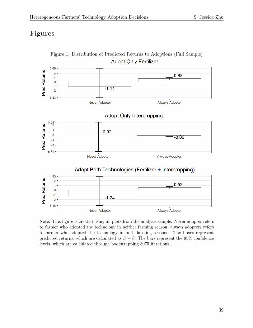
Heterogeneous Farmers’ Technology Adoption Decisions S. Jessica Zhu
Figures
Figure 1: Distribution of Predicted Returns to Adoptions (Full Sample)
Note: This figure is created using all plots from the analysis sample. Never adopter refersto farmer who adopted the technology in neither farming season; always adopters refersto farmer who adopted the technology in both farming seasons. The boxes representpredicted returns, which are calculated as β + θ. The bars represent the 95% confidencelevels, which are calculated through bootstrapping 3075 iterations.
39
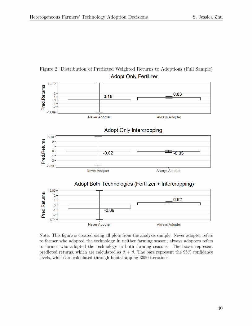
Heterogeneous Farmers’ Technology Adoption Decisions S. Jessica Zhu
Figure 2: Distribution of Predicted Weighted Returns to Adoptions (Full Sample)
Note: This figure is created using all plots from the analysis sample. Never adopter refersto farmer who adopted the technology in neither farming season; always adopters refersto farmer who adopted the technology in both farming seasons. The boxes representpredicted returns, which are calculated as β + θ. The bars represent the 95% confidencelevels, which are calculated through bootstrapping 3050 iterations.
40
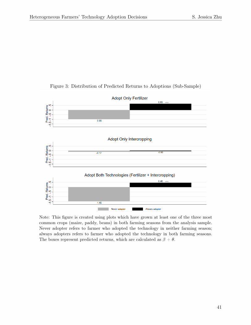
Heterogeneous Farmers’ Technology Adoption Decisions S. Jessica Zhu
Figure 3: Distribution of Predicted Returns to Adoptions (Sub-Sample)
Note: This figure is created using plots which have grown at least one of the three mostcommon crops (maize, paddy, beans) in both farming seasons from the analysis sample.Never adopter refers to farmer who adopted the technology in neither farming season;always adopters refers to farmer who adopted the technology in both farming seasons.The boxes represent predicted returns, which are calculated as β + θ.
41
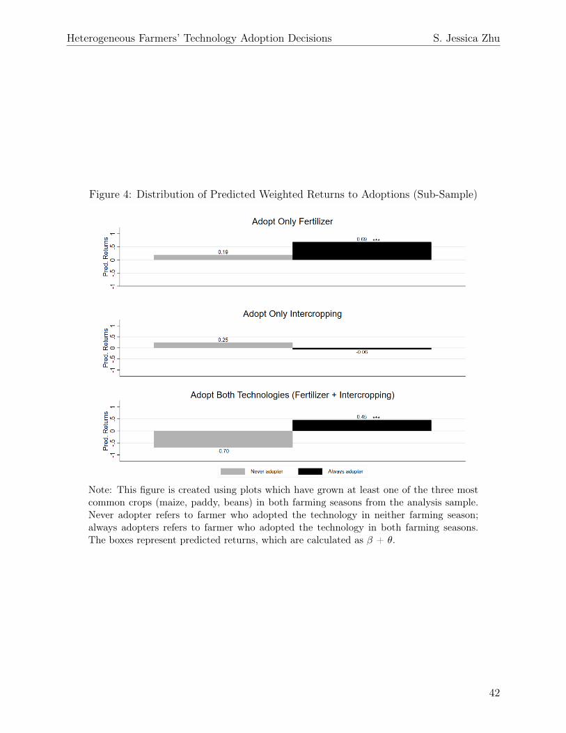
Heterogeneous Farmers’ Technology Adoption Decisions S. Jessica Zhu
Figure 4: Distribution of Predicted Weighted Returns to Adoptions (Sub-Sample)
Note: This figure is created using plots which have grown at least one of the three mostcommon crops (maize, paddy, beans) in both farming seasons from the analysis sample.Never adopter refers to farmer who adopted the technology in neither farming season;always adopters refers to farmer who adopted the technology in both farming seasons.The boxes represent predicted returns, which are calculated as β + θ.
42
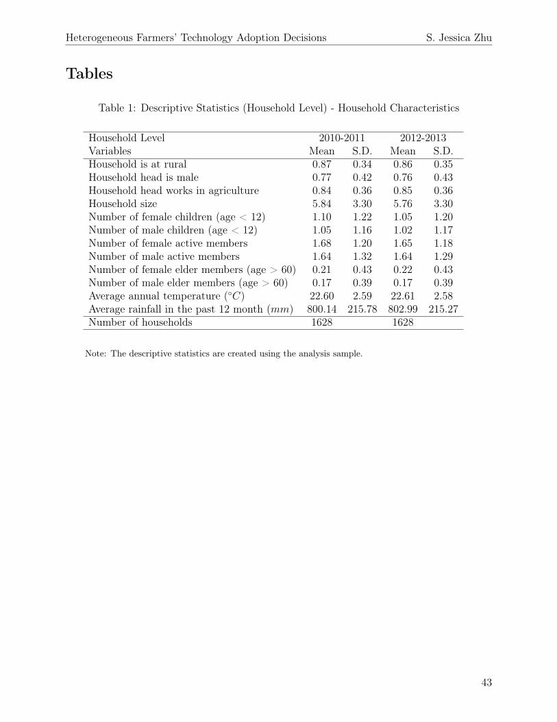
Heterogeneous Farmers’ Technology Adoption Decisions S. Jessica Zhu
Tables
Table 1: Descriptive Statistics (Household Level) - Household Characteristics
Household Level 2010-2011 2012-2013Variables Mean S.D. Mean S.D.Household is at rural 0.87 0.34 0.86 0.35Household head is male 0.77 0.42 0.76 0.43Household head works in agriculture 0.84 0.36 0.85 0.36Household size 5.84 3.30 5.76 3.30Number of female children (age < 12) 1.10 1.22 1.05 1.20Number of male children (age < 12) 1.05 1.16 1.02 1.17Number of female active members 1.68 1.20 1.65 1.18Number of male active members 1.64 1.32 1.64 1.29Number of female elder members (age > 60) 0.21 0.43 0.22 0.43Number of male elder members (age > 60) 0.17 0.39 0.17 0.39Average annual temperature (◦C) 22.60 2.59 22.61 2.58Average rainfall in the past 12 month (mm) 800.14 215.78 802.99 215.27Number of households 1628 1628
Note: The descriptive statistics are created using the analysis sample.
43
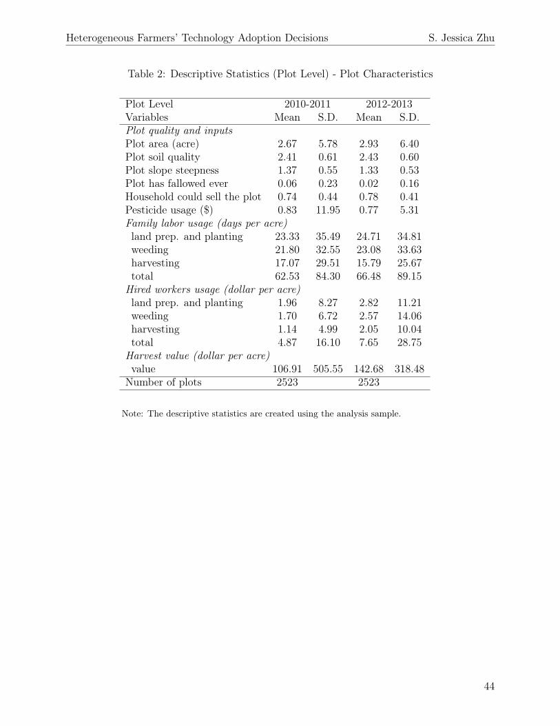
Heterogeneous Farmers’ Technology Adoption Decisions S. Jessica Zhu
Table 2: Descriptive Statistics (Plot Level) - Plot Characteristics
Plot Level 2010-2011 2012-2013Variables Mean S.D. Mean S.D.Plot quality and inputsPlot area (acre) 2.67 5.78 2.93 6.40Plot soil quality 2.41 0.61 2.43 0.60Plot slope steepness 1.37 0.55 1.33 0.53Plot has fallowed ever 0.06 0.23 0.02 0.16Household could sell the plot 0.74 0.44 0.78 0.41Pesticide usage ($) 0.83 11.95 0.77 5.31Family labor usage (days per acre)land prep. and planting 23.33 35.49 24.71 34.81weeding 21.80 32.55 23.08 33.63harvesting 17.07 29.51 15.79 25.67total 62.53 84.30 66.48 89.15
Hired workers usage (dollar per acre)land prep. and planting 1.96 8.27 2.82 11.21weeding 1.70 6.72 2.57 14.06harvesting 1.14 4.99 2.05 10.04total 4.87 16.10 7.65 28.75
Harvest value (dollar per acre)value 106.91 505.55 142.68 318.48
Number of plots 2523 2523
Note: The descriptive statistics are created using the analysis sample.
44
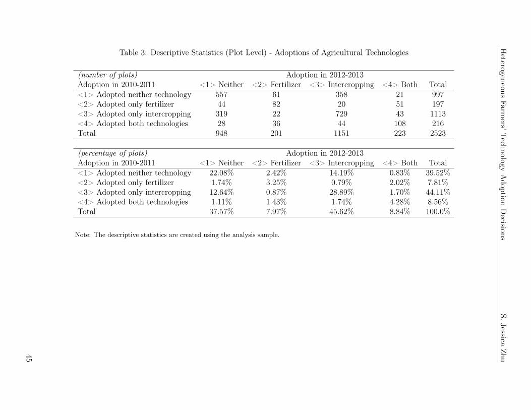
Heterogeneous
Farmers’Technology
Adoption
Decisions
S.JessicaZhu
Table 3: Descriptive Statistics (Plot Level) - Adoptions of Agricultural Technologies
(number of plots) Adoption in 2012-2013Adoption in 2010-2011 <1> Neither <2> Fertilizer <3> Intercropping <4> Both Total<1> Adopted neither technology 557 61 358 21 997<2> Adopted only fertilizer 44 82 20 51 197<3> Adopted only intercropping 319 22 729 43 1113<4> Adopted both technologies 28 36 44 108 216Total 948 201 1151 223 2523
(percentage of plots) Adoption in 2012-2013Adoption in 2010-2011 <1> Neither <2> Fertilizer <3> Intercropping <4> Both Total<1> Adopted neither technology 22.08% 2.42% 14.19% 0.83% 39.52%<2> Adopted only fertilizer 1.74% 3.25% 0.79% 2.02% 7.81%<3> Adopted only intercropping 12.64% 0.87% 28.89% 1.70% 44.11%<4> Adopted both technologies 1.11% 1.43% 1.74% 4.28% 8.56%Total 37.57% 7.97% 45.62% 8.84% 100.0%
Note: The descriptive statistics are created using the analysis sample.
45
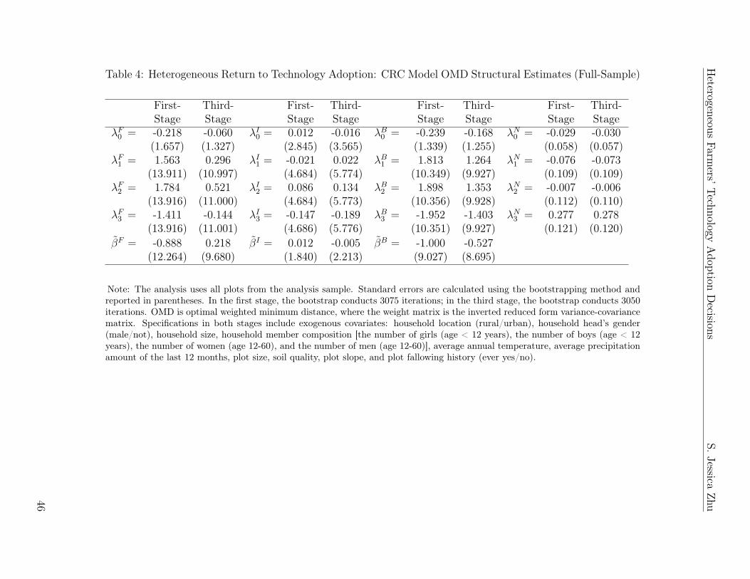
Heterogeneous
Farmers’Technology
Adoption
Decisions
S.JessicaZhu
Table 4: Heterogeneous Return to Technology Adoption: CRC Model OMD Structural Estimates (Full-Sample)
First- Third- First- Third- First- Third- First- Third-Stage Stage Stage Stage Stage Stage Stage Stage
λF0 = -0.218 -0.060 λI0 = 0.012 -0.016 λB0 = -0.239 -0.168 λN0 = -0.029 -0.030(1.657) (1.327) (2.845) (3.565) (1.339) (1.255) (0.058) (0.057)
λF1 = 1.563 0.296 λI1 = -0.021 0.022 λB1 = 1.813 1.264 λN1 = -0.076 -0.073(13.911) (10.997) (4.684) (5.774) (10.349) (9.927) (0.109) (0.109)
λF2 = 1.784 0.521 λI2 = 0.086 0.134 λB2 = 1.898 1.353 λN2 = -0.007 -0.006(13.916) (11.000) (4.684) (5.773) (10.356) (9.928) (0.112) (0.110)
λF3 = -1.411 -0.144 λI3 = -0.147 -0.189 λB3 = -1.952 -1.403 λN3 = 0.277 0.278(13.916) (11.001) (4.686) (5.776) (10.351) (9.927) (0.121) (0.120)
βF = -0.888 0.218 βI = 0.012 -0.005 βB = -1.000 -0.527(12.264) (9.680) (1.840) (2.213) (9.027) (8.695)
Note: The analysis uses all plots from the analysis sample. Standard errors are calculated using the bootstrapping method andreported in parentheses. In the first stage, the bootstrap conducts 3075 iterations; in the third stage, the bootstrap conducts 3050iterations. OMD is optimal weighted minimum distance, where the weight matrix is the inverted reduced form variance-covariancematrix. Specifications in both stages include exogenous covariates: household location (rural/urban), household head’s gender(male/not), household size, household member composition [the number of girls (age < 12 years), the number of boys (age < 12years), the number of women (age 12-60), and the number of men (age 12-60)], average annual temperature, average precipitationamount of the last 12 months, plot size, soil quality, plot slope, and plot fallowing history (ever yes/no).
46
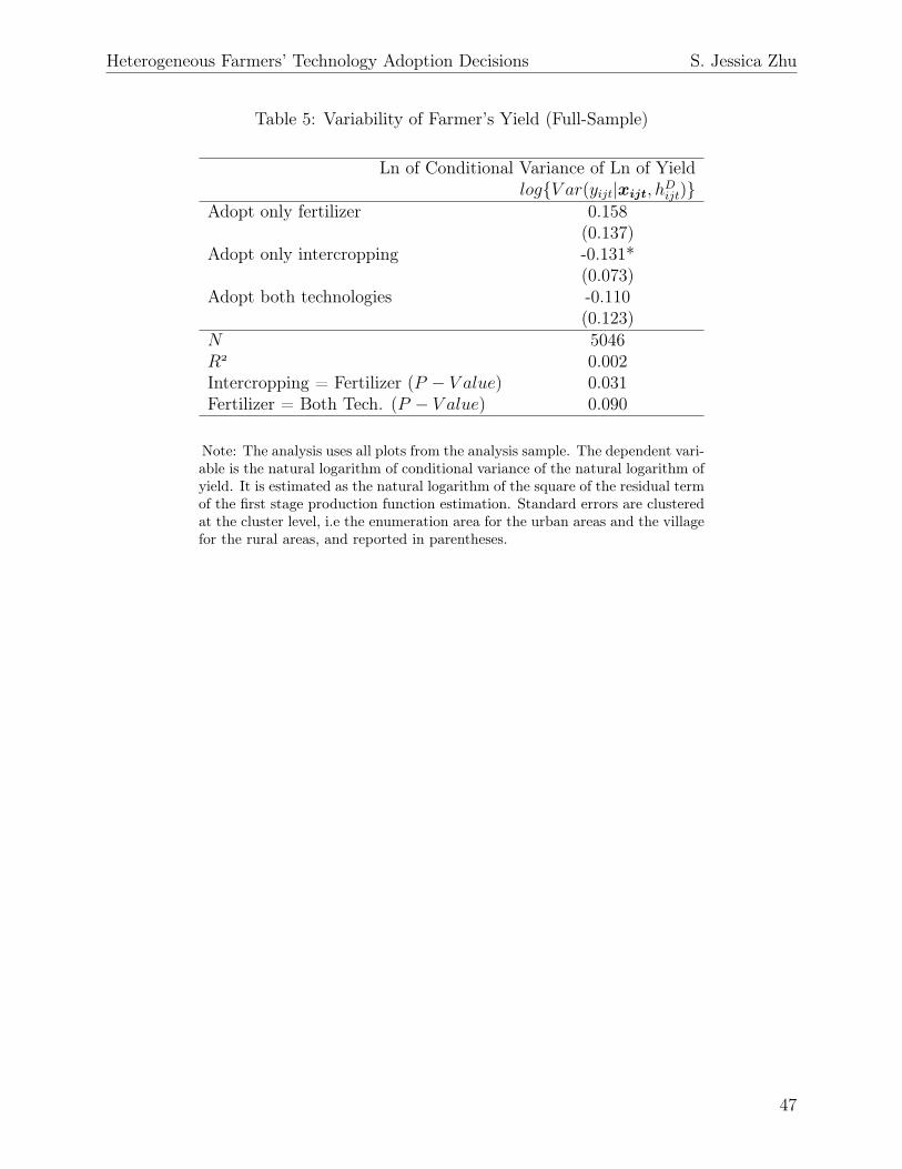
Heterogeneous Farmers’ Technology Adoption Decisions S. Jessica Zhu
Table 5: Variability of Farmer’s Yield (Full-Sample)
Ln of Conditional Variance of Ln of Yieldlog{V ar(yijt|xijt, h
Dijt)}
Adopt only fertilizer 0.158(0.137)
Adopt only intercropping -0.131*(0.073)
Adopt both technologies -0.110(0.123)
N 5046R 0.002Intercropping = Fertilizer (P − V alue) 0.031Fertilizer = Both Tech. (P − V alue) 0.090
Note: The analysis uses all plots from the analysis sample. The dependent vari-able is the natural logarithm of conditional variance of the natural logarithm ofyield. It is estimated as the natural logarithm of the square of the residual termof the first stage production function estimation. Standard errors are clusteredat the cluster level, i.e the enumeration area for the urban areas and the villagefor the rural areas, and reported in parentheses.
47
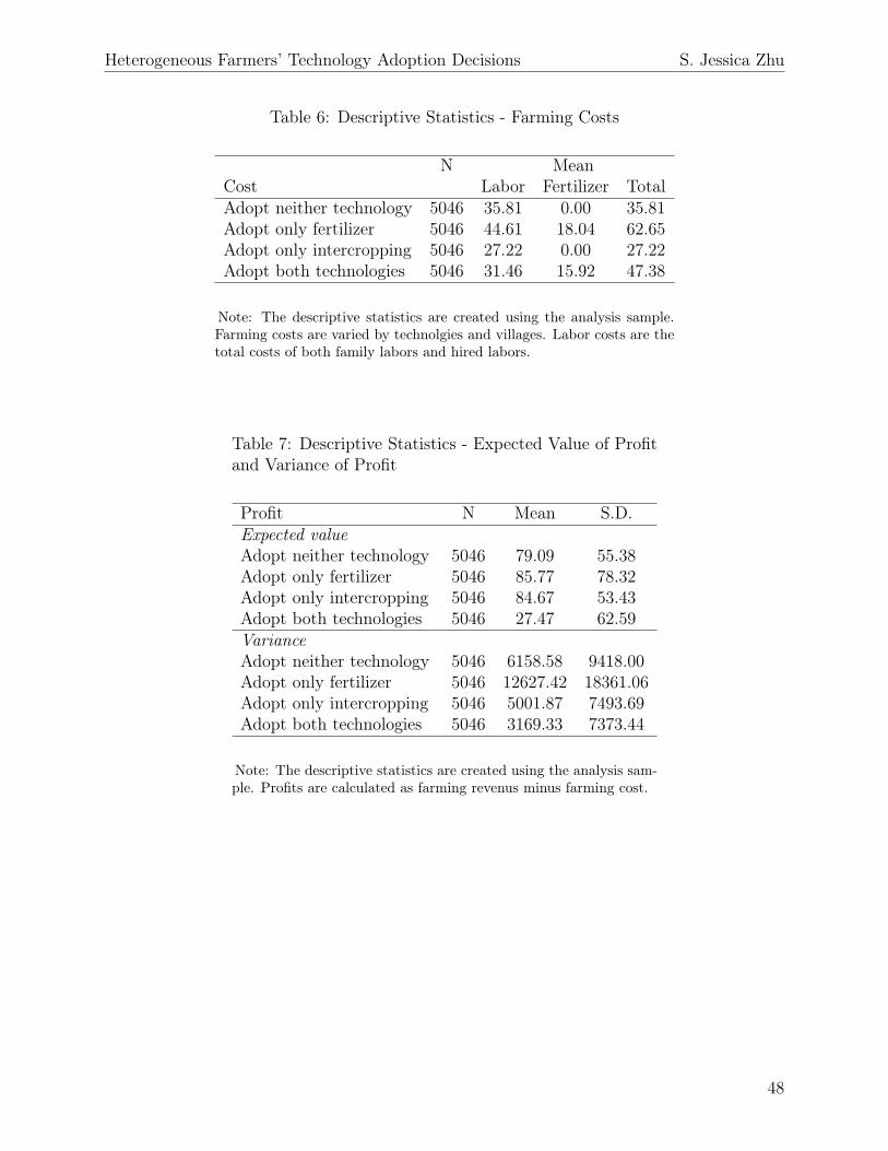
Heterogeneous Farmers’ Technology Adoption Decisions S. Jessica Zhu
Table 6: Descriptive Statistics - Farming Costs
N MeanCost Labor Fertilizer TotalAdopt neither technology 5046 35.81 0.00 35.81Adopt only fertilizer 5046 44.61 18.04 62.65Adopt only intercropping 5046 27.22 0.00 27.22Adopt both technologies 5046 31.46 15.92 47.38
Note: The descriptive statistics are created using the analysis sample.Farming costs are varied by technolgies and villages. Labor costs are thetotal costs of both family labors and hired labors.
Table 7: Descriptive Statistics - Expected Value of Profitand Variance of Profit
Profit N Mean S.D.Expected valueAdopt neither technology 5046 79.09 55.38Adopt only fertilizer 5046 85.77 78.32Adopt only intercropping 5046 84.67 53.43Adopt both technologies 5046 27.47 62.59VarianceAdopt neither technology 5046 6158.58 9418.00Adopt only fertilizer 5046 12627.42 18361.06Adopt only intercropping 5046 5001.87 7493.69Adopt both technologies 5046 3169.33 7373.44
Note: The descriptive statistics are created using the analysis sam-ple. Profits are calculated as farming revenus minus farming cost.
48
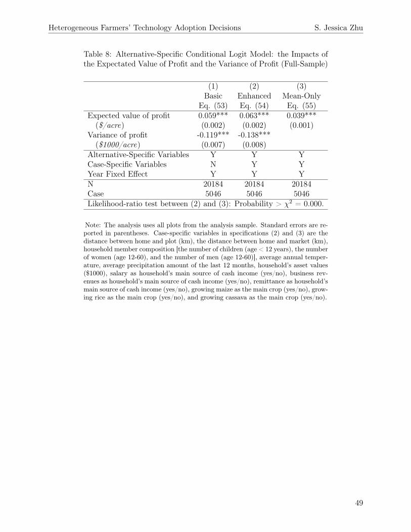
Heterogeneous Farmers’ Technology Adoption Decisions S. Jessica Zhu
Table 8: Alternative-Specific Conditional Logit Model: the Impacts ofthe Expectated Value of Profit and the Variance of Profit (Full-Sample)
(1) (2) (3)Basic Enhanced Mean-Only
Eq. (53) Eq. (54) Eq. (55)Expected value of profit 0.059*** 0.063*** 0.039***($/acre) (0.002) (0.002) (0.001)
Variance of profit -0.119*** -0.138***($1000/acre) (0.007) (0.008)
Alternative-Specific Variables Y Y YCase-Specific Variables N Y YYear Fixed Effect Y Y YN 20184 20184 20184Case 5046 5046 5046Likelihood-ratio test between (2) and (3): Probability > χ2 = 0.000.
Note: The analysis uses all plots from the analysis sample. Standard errors are re-ported in parentheses. Case-specific variables in specifications (2) and (3) are thedistance between home and plot (km), the distance between home and market (km),household member composition [the number of children (age < 12 years), the numberof women (age 12-60), and the number of men (age 12-60)], average annual temper-ature, average precipitation amount of the last 12 months, household’s asset values($1000), salary as household’s main source of cash income (yes/no), business rev-enues as household’s main source of cash income (yes/no), remittance as household’smain source of cash income (yes/no), growing maize as the main crop (yes/no), grow-ing rice as the main crop (yes/no), and growing cassava as the main crop (yes/no).
49
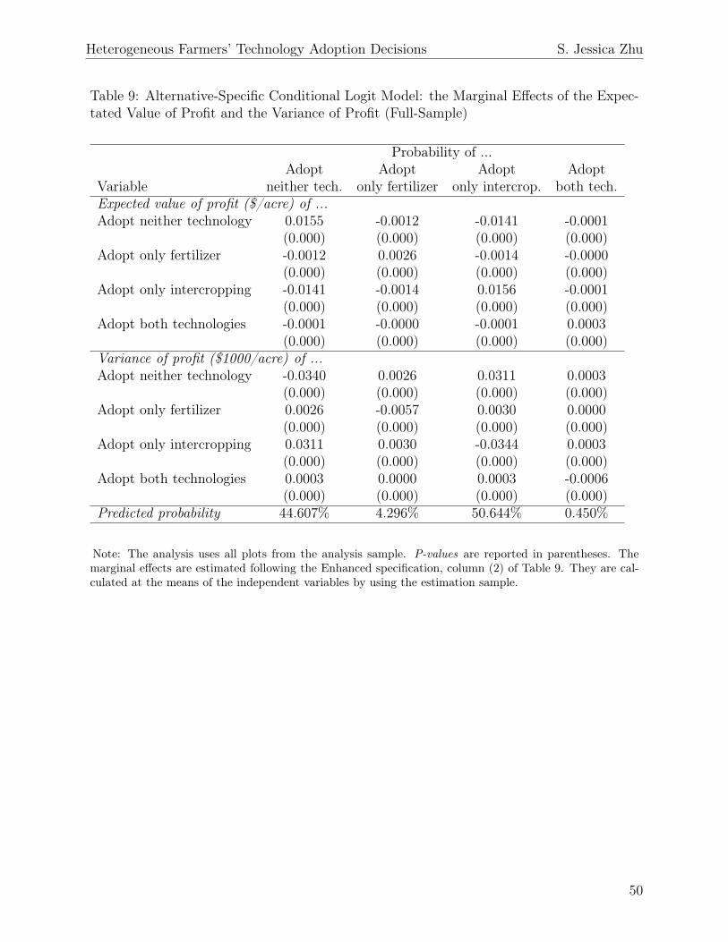
Heterogeneous Farmers’ Technology Adoption Decisions S. Jessica Zhu
Table 9: Alternative-Specific Conditional Logit Model: the Marginal Effects of the Expec-tated Value of Profit and the Variance of Profit (Full-Sample)
Probability of ...Adopt Adopt Adopt Adopt
Variable neither tech. only fertilizer only intercrop. both tech.Expected value of profit ($/acre) of ...Adopt neither technology 0.0155 -0.0012 -0.0141 -0.0001
(0.000) (0.000) (0.000) (0.000)Adopt only fertilizer -0.0012 0.0026 -0.0014 -0.0000
(0.000) (0.000) (0.000) (0.000)Adopt only intercropping -0.0141 -0.0014 0.0156 -0.0001
(0.000) (0.000) (0.000) (0.000)Adopt both technologies -0.0001 -0.0000 -0.0001 0.0003
(0.000) (0.000) (0.000) (0.000)Variance of profit ($1000/acre) of ...Adopt neither technology -0.0340 0.0026 0.0311 0.0003
(0.000) (0.000) (0.000) (0.000)Adopt only fertilizer 0.0026 -0.0057 0.0030 0.0000
(0.000) (0.000) (0.000) (0.000)Adopt only intercropping 0.0311 0.0030 -0.0344 0.0003
(0.000) (0.000) (0.000) (0.000)Adopt both technologies 0.0003 0.0000 0.0003 -0.0006
(0.000) (0.000) (0.000) (0.000)Predicted probability 44.607% 4.296% 50.644% 0.450%
Note: The analysis uses all plots from the analysis sample. P-values are reported in parentheses. Themarginal effects are estimated following the Enhanced specification, column (2) of Table 9. They are cal-culated at the means of the independent variables by using the estimation sample.
50
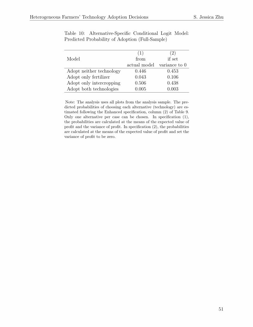
Heterogeneous Farmers’ Technology Adoption Decisions S. Jessica Zhu
Table 10: Alternative-Specific Conditional Logit Model:Predicted Probability of Adoption (Full-Sample)
(1) (2)Model from if set
actual model variance to 0Adopt neither technology 0.446 0.453Adopt only fertilizer 0.043 0.106Adopt only intercropping 0.506 0.438Adopt both technologies 0.005 0.003
Note: The analysis uses all plots from the analysis sample. The pre-dicted probabilities of choosing each alternative (technology) are es-timated following the Enhanced specification, column (2) of Table 9.Only one alternative per case can be chosen. In specification (1),the probabilities are calculated at the means of the expected value ofprofit and the variance of profit. In specification (2), the probabilitiesare calculated at the means of the expected value of profit and set thevariance of profit to be zero.
51
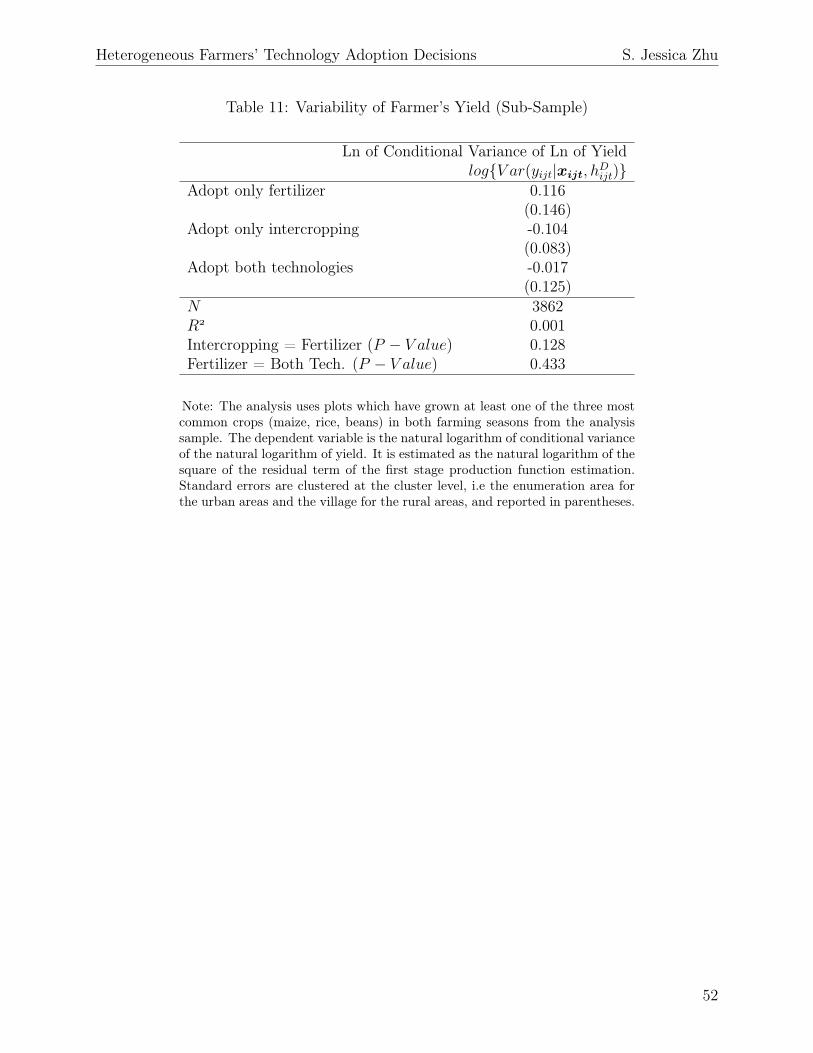
Heterogeneous Farmers’ Technology Adoption Decisions S. Jessica Zhu
Table 11: Variability of Farmer’s Yield (Sub-Sample)
Ln of Conditional Variance of Ln of Yieldlog{V ar(yijt|xijt, h
Dijt)}
Adopt only fertilizer 0.116(0.146)
Adopt only intercropping -0.104(0.083)
Adopt both technologies -0.017(0.125)
N 3862R 0.001Intercropping = Fertilizer (P − V alue) 0.128Fertilizer = Both Tech. (P − V alue) 0.433
Note: The analysis uses plots which have grown at least one of the three mostcommon crops (maize, rice, beans) in both farming seasons from the analysissample. The dependent variable is the natural logarithm of conditional varianceof the natural logarithm of yield. It is estimated as the natural logarithm of thesquare of the residual term of the first stage production function estimation.Standard errors are clustered at the cluster level, i.e the enumeration area forthe urban areas and the village for the rural areas, and reported in parentheses.
52
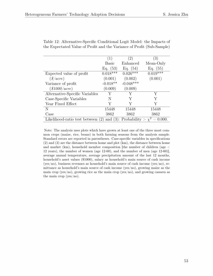
Heterogeneous Farmers’ Technology Adoption Decisions S. Jessica Zhu
Table 12: Alternative-Specific Conditional Logit Model: the Impacts ofthe Expectated Value of Profit and the Variance of Profit (Sub-Sample)
(1) (2) (3)Basic Enhanced Mean-Only
Eq. (53) Eq. (54) Eq. (55)Expected value of profit 0.018*** 0.026*** 0.019***($/acre) (0.001) (0.002) (0.001)
Variance of profit -0.018** -0.048***($1000/acre) (0.009) (0.009)
Alternative-Specific Variables Y Y YCase-Specific Variables N Y YYear Fixed Effect Y Y YN 15448 15448 15448Case 3862 3862 3862Likelihood-ratio test between (2) and (3): Probability > χ2 = 0.000.
Note: The analysis uses plots which have grown at least one of the three most com-mon crops (maize, rice, beans) in both farming seasons from the analysis sample.Standard errors are reported in parentheses. Case-specific variables in specifications(2) and (3) are the distance between home and plot (km), the distance between homeand market (km), household member composition [the number of children (age <12 years), the number of women (age 12-60), and the number of men (age 12-60)],average annual temperature, average precipitation amount of the last 12 months,household’s asset values ($1000), salary as household’s main source of cash income(yes/no), business revenues as household’s main source of cash income (yes/no), re-mittance as household’s main source of cash income (yes/no), growing maize as themain crop (yes/no), growing rice as the main crop (yes/no), and growing cassava asthe main crop (yes/no).
53
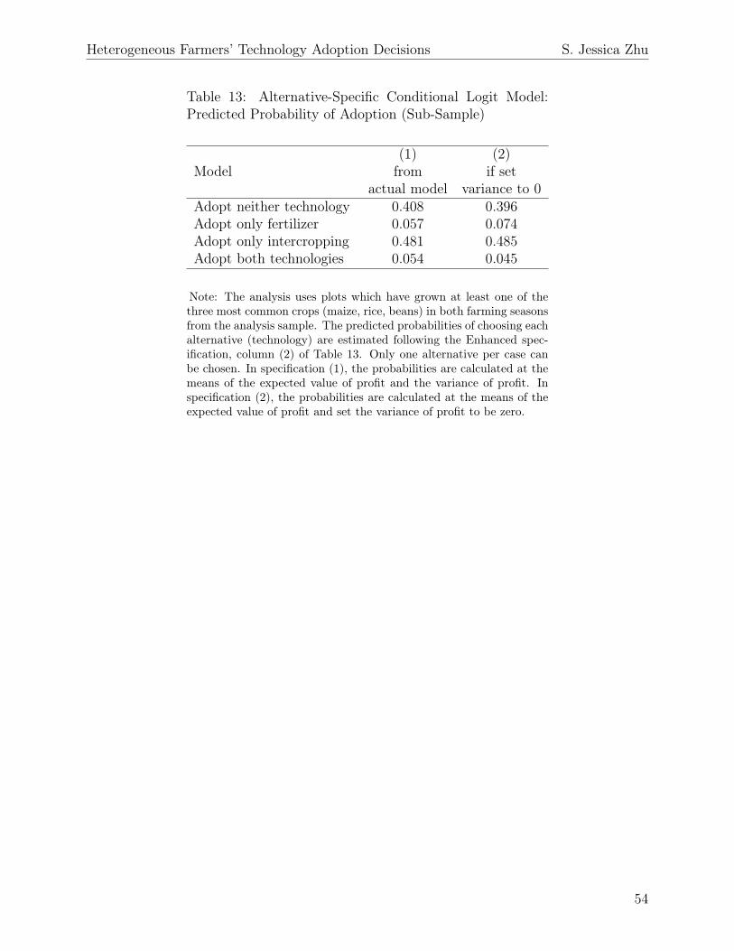
Heterogeneous Farmers’ Technology Adoption Decisions S. Jessica Zhu
Table 13: Alternative-Specific Conditional Logit Model:Predicted Probability of Adoption (Sub-Sample)
(1) (2)Model from if set
actual model variance to 0Adopt neither technology 0.408 0.396Adopt only fertilizer 0.057 0.074Adopt only intercropping 0.481 0.485Adopt both technologies 0.054 0.045
Note: The analysis uses plots which have grown at least one of thethree most common crops (maize, rice, beans) in both farming seasonsfrom the analysis sample. The predicted probabilities of choosing eachalternative (technology) are estimated following the Enhanced spec-ification, column (2) of Table 13. Only one alternative per case canbe chosen. In specification (1), the probabilities are calculated at themeans of the expected value of profit and the variance of profit. Inspecification (2), the probabilities are calculated at the means of theexpected value of profit and set the variance of profit to be zero.
54
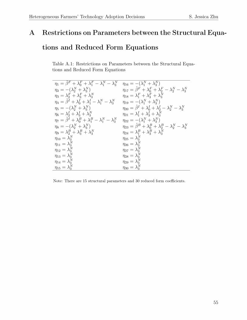
Heterogeneous Farmers’ Technology Adoption Decisions S. Jessica Zhu
A Restrictions on Parameters between the Structural Equa-
tions and Reduced Form Equations
Table A.1: Restrictions on Parameters between the Structural Equa-tions and Reduced Form Equations
η1 = βF + λF0 + λF1 − λN1 − λN3 η16 = −(λN1 + λN3 )
η2 = −(λN2 + λN3 ) η17 = βF + λF0 + λF2 − λN2 − λN3η3 = λF2 + λF3 + λN3 η18 = λF1 + λF3 + λN3η4 = βI + λI0 + λI1 − λN1 − λN3 η19 = −(λN1 + λN3 )
η5 = −(λN2 + λN3 ) η20 = βI + λI0 + λI2 − λN2 − λN3η6 = λI2 + λI3 + λN3 η21 = λI1 + λI3 + λN3η7 = βI + λB0 + λB1 − λN1 − λN3 η22 = −(λN1 + λN3 )
η8 = −(λN2 + λN3 ) η23 = βB + λB0 + λB2 − λN2 − λN3η9 = λB2 + λB3 + λN3 η24 = λB1 + λB3 + λN3η10 = λN3 η25 = λN3η11 = λN3 η26 = λN3η12 = λN3 η27 = λN3η13 = λN3 η28 = λN3η14 = λN3 η29 = λN3η15 = λN3 η30 = λN3
Note: There are 15 structural parameters and 30 reduced form coefficients.
55
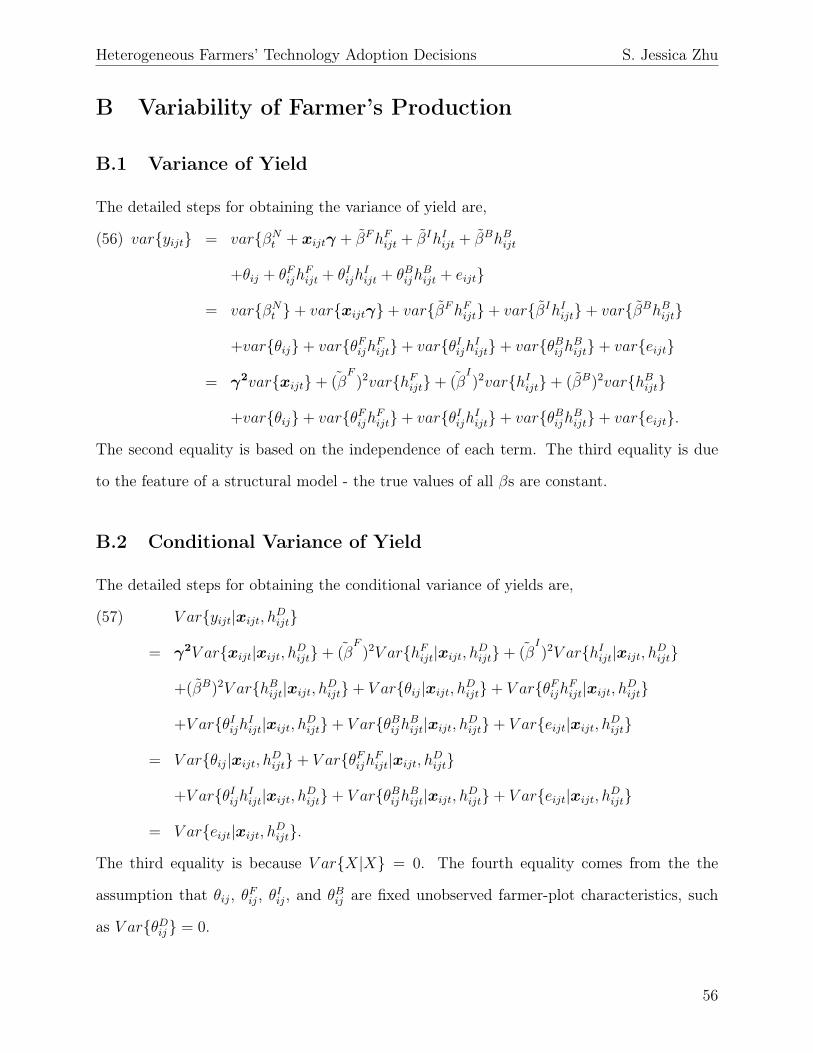
Heterogeneous Farmers’ Technology Adoption Decisions S. Jessica Zhu
B Variability of Farmer’s Production
B.1 Variance of Yield
The detailed steps for obtaining the variance of yield are,
var{yijt} = var{βNt + xijtγ + βFhFijt + βIhIijt + βBhBijt(56)
+θij + θFijhFijt + θIijh
Iijt + θBijh
Bijt + eijt}
= var{βNt }+ var{xijtγ}+ var{βFhFijt}+ var{βIhIijt}+ var{βBhBijt}
+var{θij}+ var{θFijhFijt}+ var{θIijhIijt}+ var{θBijhBijt}+ var{eijt}
= γ2var{xijt}+ (βF
)2var{hFijt}+ (βI)2var{hIijt}+ (βB)2var{hBijt}
+var{θij}+ var{θFijhFijt}+ var{θIijhIijt}+ var{θBijhBijt}+ var{eijt}.
The second equality is based on the independence of each term. The third equality is due
to the feature of a structural model - the true values of all βs are constant.
B.2 Conditional Variance of Yield
The detailed steps for obtaining the conditional variance of yields are,
V ar{yijt|xijt, hDijt}(57)
= γ2V ar{xijt|xijt, hDijt}+ (βF
)2V ar{hFijt|xijt, hDijt}+ (βI)2V ar{hIijt|xijt, hDijt}
+(βB)2V ar{hBijt|xijt, hDijt}+ V ar{θij|xijt, hDijt}+ V ar{θFijhFijt|xijt, hDijt}
+V ar{θIijhIijt|xijt, hDijt}+ V ar{θBijhBijt|xijt, hDijt}+ V ar{eijt|xijt, hDijt}
= V ar{θij|xijt, hDijt}+ V ar{θFijhFijt|xijt, hDijt}
+V ar{θIijhIijt|xijt, hDijt}+ V ar{θBijhBijt|xijt, hDijt}+ V ar{eijt|xijt, hDijt}
= V ar{eijt|xijt, hDijt}.
The third equality is because V ar{X|X} = 0. The fourth equality comes from the the
assumption that θij, θFij , θIij, and θBij are fixed unobserved farmer-plot characteristics, such
as V ar{θDij} = 0.
56
Heterogeneous Farmers’ Technology Adoption Decisions S. Jessica Zhu
After substituting the definition of error term in to the previous equation, I get the
elaborated conditional variance of yields as
V ar{yijt|xijt, hDijt} = V ar{eijt|xijt, hDijt}(58)
= V ar{∑d∈D
(αd)12hdijtεijt|xijt, hDijt}
=∑d∈D
V ar{(αd)12hdijtεijt|xijt, hDijt}
=∑d∈D
{E[((αd)12hdijtεijt)
2]− [E((αd)12hdijtεijt)]
2|xijt, hDijt}
=∑d∈D
{E[((αd)12hdijt)
2]E[ε2ijt]− [E((αd)12hdijt)E(εijt)]
2|xijt, hDijt}
=∑d∈D
{E[((αd)12hdijt)
2]|xijt, hDijt}
=∑d∈D
{E[αd(hdijt)2]|xijt, hDijt}
= E[αN(hNijt)2|xijt, hDijt] + E[αF (hFijt)
2|xijt, hDijt]
+E[αI(hIijt)2|xijt, hDijt] + E[αB(hBijt)
2|xijt, hDijt]
= E[αNhNijt|xijt, hDijt] + E[αFhFijt|xijt, hDijt]
+E[αIhIijt|xijt, hDijt] + E[αBhBijt|xijt, hDijt],
where E[ε2ijt] = 1 because V ar[εijt] = E[ε2ijt]− [E(εijt)]2 = 1 and E(εijt) = 0.
57
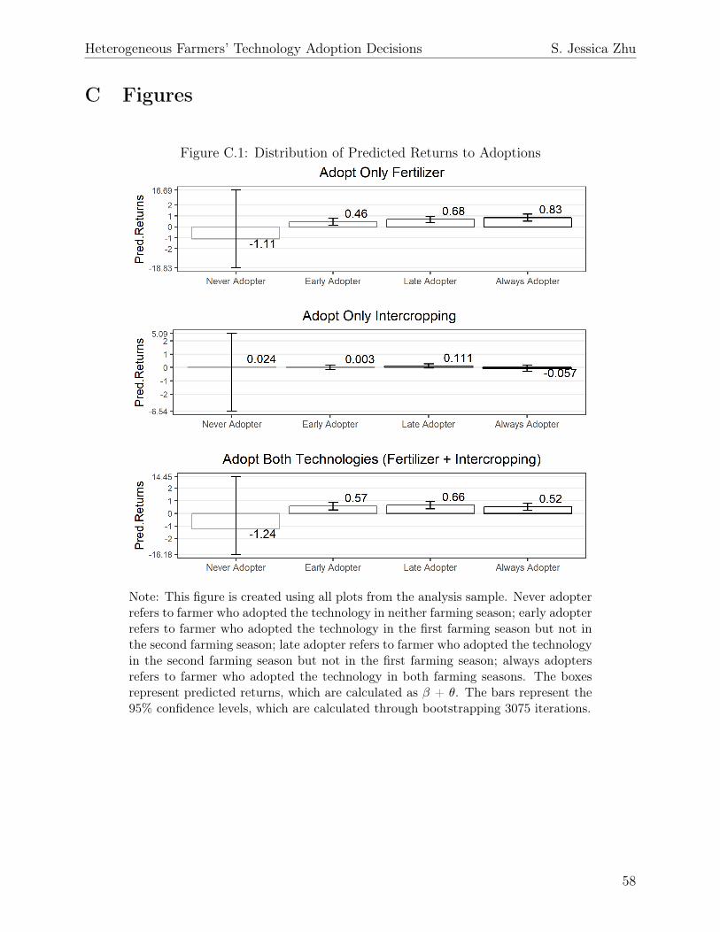
Heterogeneous Farmers’ Technology Adoption Decisions S. Jessica Zhu
C Figures
Figure C.1: Distribution of Predicted Returns to Adoptions
Note: This figure is created using all plots from the analysis sample. Never adopterrefers to farmer who adopted the technology in neither farming season; early adopterrefers to farmer who adopted the technology in the first farming season but not inthe second farming season; late adopter refers to farmer who adopted the technologyin the second farming season but not in the first farming season; always adoptersrefers to farmer who adopted the technology in both farming seasons. The boxesrepresent predicted returns, which are calculated as β + θ. The bars represent the95% confidence levels, which are calculated through bootstrapping 3075 iterations.
58
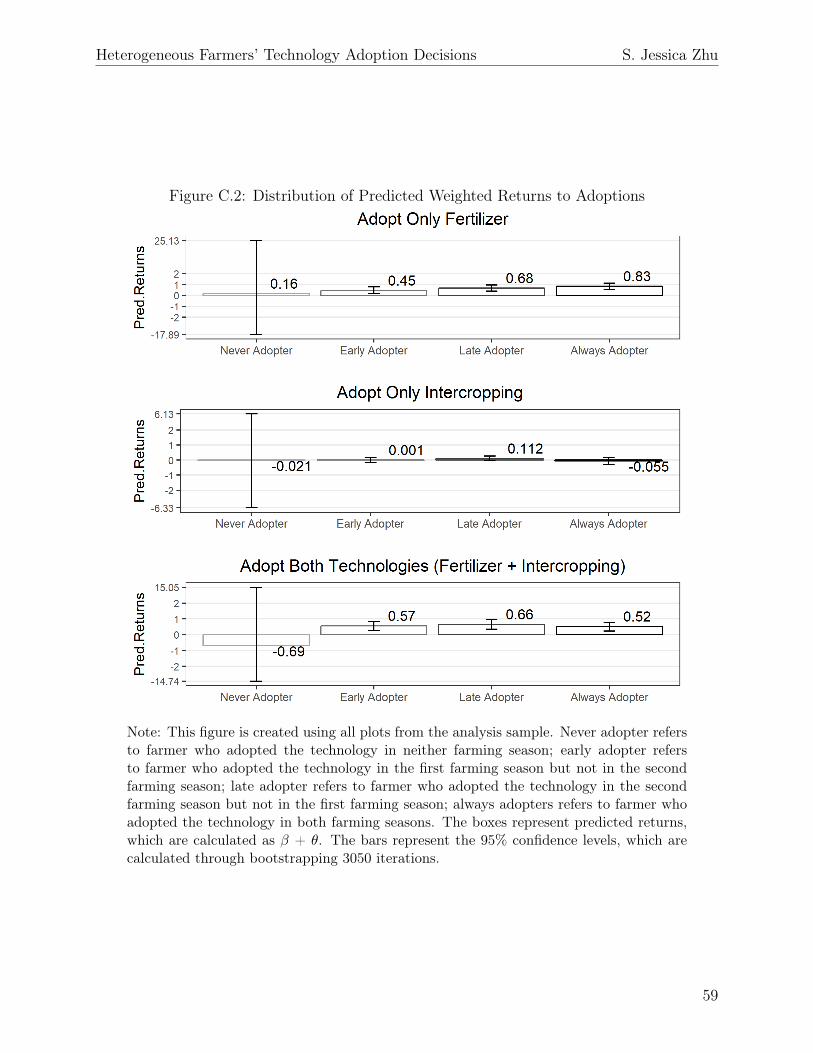
Heterogeneous Farmers’ Technology Adoption Decisions S. Jessica Zhu
Figure C.2: Distribution of Predicted Weighted Returns to Adoptions
Note: This figure is created using all plots from the analysis sample. Never adopter refersto farmer who adopted the technology in neither farming season; early adopter refersto farmer who adopted the technology in the first farming season but not in the secondfarming season; late adopter refers to farmer who adopted the technology in the secondfarming season but not in the first farming season; always adopters refers to farmer whoadopted the technology in both farming seasons. The boxes represent predicted returns,which are calculated as β + θ. The bars represent the 95% confidence levels, which arecalculated through bootstrapping 3050 iterations.
59
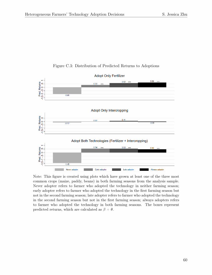
Heterogeneous Farmers’ Technology Adoption Decisions S. Jessica Zhu
Figure C.3: Distribution of Predicted Returns to Adoptions
Note: This figure is created using plots which have grown at least one of the three mostcommon crops (maize, paddy, beans) in both farming seasons from the analysis sample.Never adopter refers to farmer who adopted the technology in neither farming season;early adopter refers to farmer who adopted the technology in the first farming season butnot in the second farming season; late adopter refers to farmer who adopted the technologyin the second farming season but not in the first farming season; always adopters refersto farmer who adopted the technology in both farming seasons. The boxes representpredicted returns, which are calculated as β + θ.
60
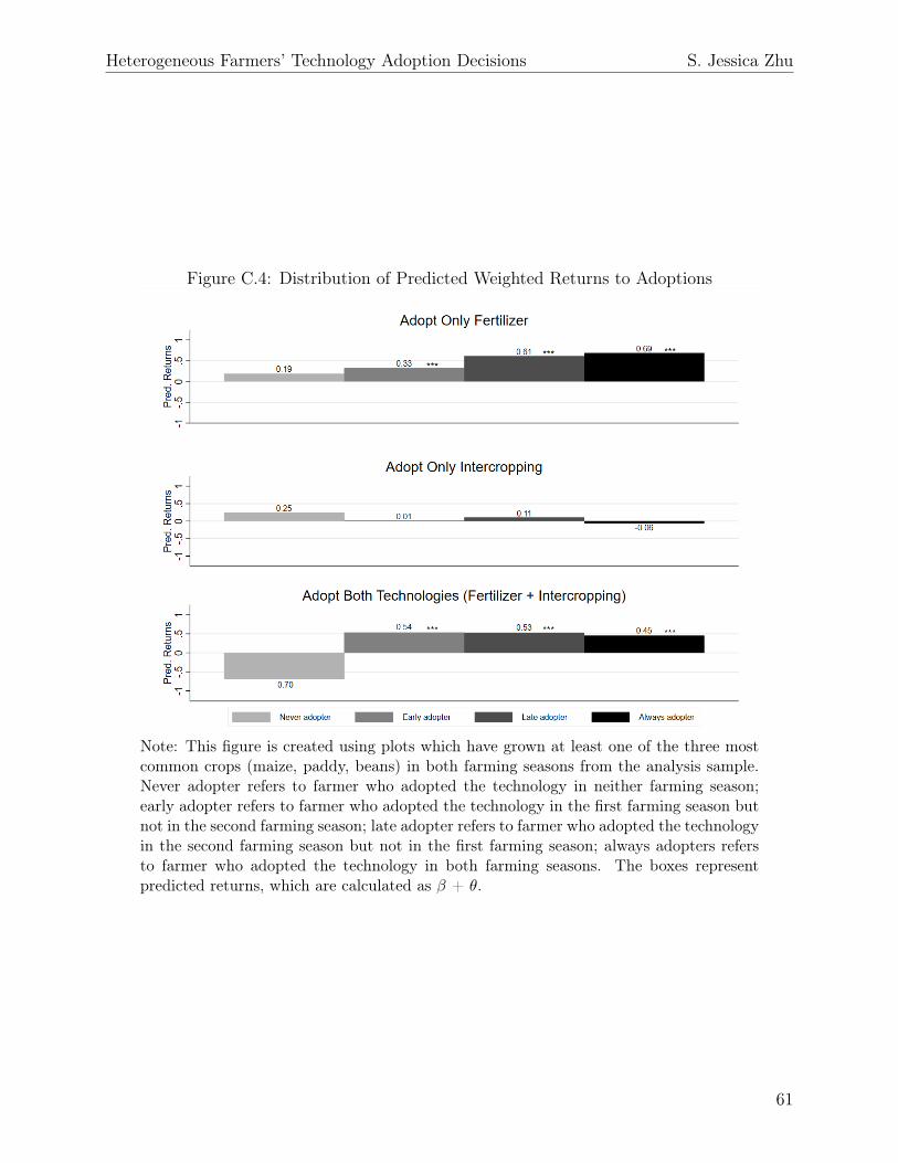
Heterogeneous Farmers’ Technology Adoption Decisions S. Jessica Zhu
Figure C.4: Distribution of Predicted Weighted Returns to Adoptions
Note: This figure is created using plots which have grown at least one of the three mostcommon crops (maize, paddy, beans) in both farming seasons from the analysis sample.Never adopter refers to farmer who adopted the technology in neither farming season;early adopter refers to farmer who adopted the technology in the first farming season butnot in the second farming season; late adopter refers to farmer who adopted the technologyin the second farming season but not in the first farming season; always adopters refersto farmer who adopted the technology in both farming seasons. The boxes representpredicted returns, which are calculated as β + θ.
61
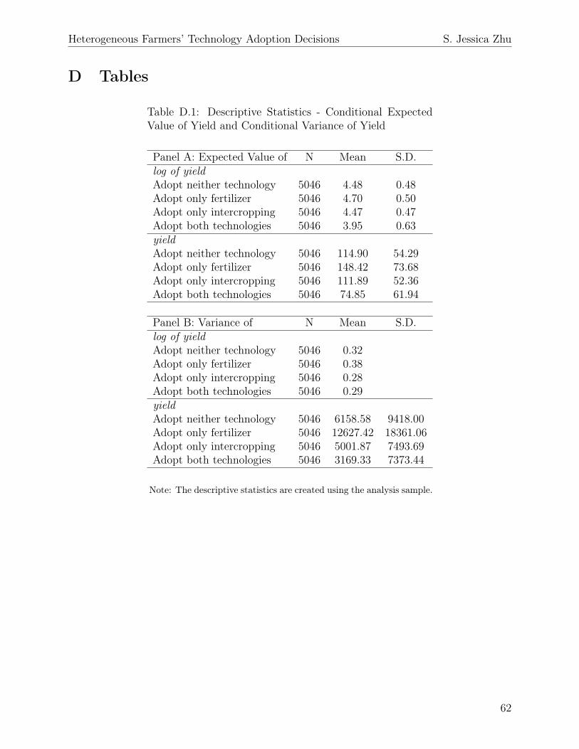
Heterogeneous Farmers’ Technology Adoption Decisions S. Jessica Zhu
D Tables
Table D.1: Descriptive Statistics - Conditional ExpectedValue of Yield and Conditional Variance of Yield
Panel A: Expected Value of N Mean S.D.log of yieldAdopt neither technology 5046 4.48 0.48Adopt only fertilizer 5046 4.70 0.50Adopt only intercropping 5046 4.47 0.47Adopt both technologies 5046 3.95 0.63yieldAdopt neither technology 5046 114.90 54.29Adopt only fertilizer 5046 148.42 73.68Adopt only intercropping 5046 111.89 52.36Adopt both technologies 5046 74.85 61.94
Panel B: Variance of N Mean S.D.log of yieldAdopt neither technology 5046 0.32Adopt only fertilizer 5046 0.38Adopt only intercropping 5046 0.28Adopt both technologies 5046 0.29yieldAdopt neither technology 5046 6158.58 9418.00Adopt only fertilizer 5046 12627.42 18361.06Adopt only intercropping 5046 5001.87 7493.69Adopt both technologies 5046 3169.33 7373.44
Note: The descriptive statistics are created using the analysis sample.
62
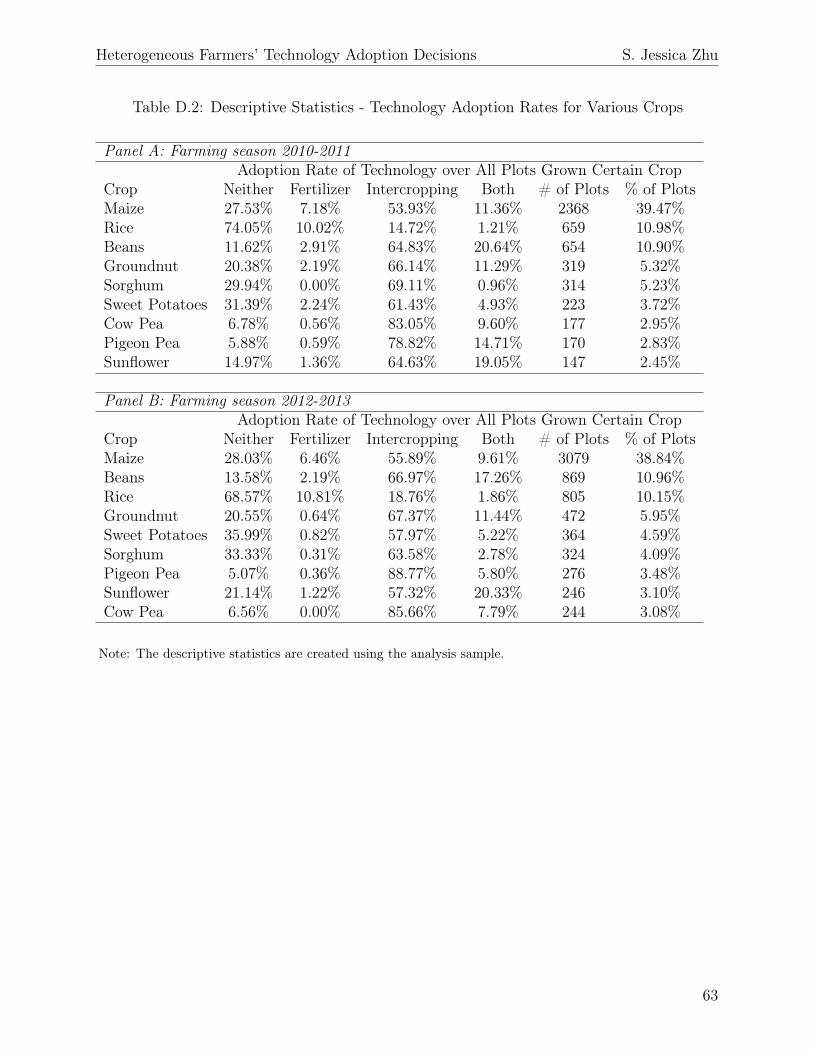
Heterogeneous Farmers’ Technology Adoption Decisions S. Jessica Zhu
Table D.2: Descriptive Statistics - Technology Adoption Rates for Various Crops
Panel A: Farming season 2010-2011Adoption Rate of Technology over All Plots Grown Certain Crop
Crop Neither Fertilizer Intercropping Both # of Plots % of PlotsMaize 27.53% 7.18% 53.93% 11.36% 2368 39.47%Rice 74.05% 10.02% 14.72% 1.21% 659 10.98%Beans 11.62% 2.91% 64.83% 20.64% 654 10.90%Groundnut 20.38% 2.19% 66.14% 11.29% 319 5.32%Sorghum 29.94% 0.00% 69.11% 0.96% 314 5.23%Sweet Potatoes 31.39% 2.24% 61.43% 4.93% 223 3.72%Cow Pea 6.78% 0.56% 83.05% 9.60% 177 2.95%Pigeon Pea 5.88% 0.59% 78.82% 14.71% 170 2.83%Sunflower 14.97% 1.36% 64.63% 19.05% 147 2.45%
Panel B: Farming season 2012-2013Adoption Rate of Technology over All Plots Grown Certain Crop
Crop Neither Fertilizer Intercropping Both # of Plots % of PlotsMaize 28.03% 6.46% 55.89% 9.61% 3079 38.84%Beans 13.58% 2.19% 66.97% 17.26% 869 10.96%Rice 68.57% 10.81% 18.76% 1.86% 805 10.15%Groundnut 20.55% 0.64% 67.37% 11.44% 472 5.95%Sweet Potatoes 35.99% 0.82% 57.97% 5.22% 364 4.59%Sorghum 33.33% 0.31% 63.58% 2.78% 324 4.09%Pigeon Pea 5.07% 0.36% 88.77% 5.80% 276 3.48%Sunflower 21.14% 1.22% 57.32% 20.33% 246 3.10%Cow Pea 6.56% 0.00% 85.66% 7.79% 244 3.08%
Note: The descriptive statistics are created using the analysis sample.
63