Embed Size (px)
Citation preview
Ce
ntr
efo
rD
yn
am
icM
ac
ro
ec
on
om
icA
na
lys
is
Heterogeneous Expectations,Optimal Monetary Policy, and theMerit of Policy Inertia
Emanuel Gasteiger
CDMA Working Paper Series No. 130814 Sep 2013JEL Classification: E52, D84Keywords: Optimal Monetary Policy, Heterogeneous Expectations, Policy Inertia
Heterogeneous Expectations, Optimal Monetary Policy,and the Merit of Policy InertiaI
Emanuel Gasteigera,⇤
aAssistant Professor, Instituto Universitario de Lisboa (ISCTE - IUL), BRU - IUL,Department of Economics, Av.a das Forcas Armadas, 1649-026 Lisboa, Portugal
Abstract
The design and analysis of optimal monetary policy is usually guided by the
paradigm of homogeneous rational expectations. Instead, we examine the dy-
namic consequences of design and implementation strategies, when the actual
economy features expectational heterogeneity. Agents have either rational or
adaptive expectations. Consequently the central bank’s ability to achieve price-
stability under heterogeneous expectations depends on its objective and imple-
mentation strategy. An expectations-based reaction function, which appropri-
ately conditions on private sector expectations, performs exceptionally well. How-
ever, once the objective introduces policy inertia, popular strategies have similar
determinacy properties, but they are less operational. This finding calls for new
implementation strategies under interest rate stabilization.
JEL codes: E52, D84
Keywords: Heterogeneous expectations, optimal monetary policy, policy iner-
tia.
II gratefully acknowledge the extensive and constructive comments and suggestions of twoanonymous referees and the editor that I incorporated into the substantially revised paper. Iam also indebted to Gerhard Sorger and Robert Kunst for sound supervision and patience.Moreover, I am grateful to Bennett T. McCallum for the insightful correspondence about cal-culating solutions to rational expectations models as well as to Seppo Honkapohja, TorstenLisson, Karl Schlag, Shoujian Zhang, and the participants of the Graduate Seminar at theUniversity of Vienna, the seminar at City University London, and the 6th PhD PresentationMeeting of the Royal Economic Society for many helpful comments. Any remaining errors arethe responsibility of the author. Financial support from Fundacao para a Ciencia e a Tecnologia(PEst-OE/EGE/UI0315/2011) is acknowledged.
⇤Corresponding author: Av.a das Forcas Armadas, 1649-026 Lisboa, Portugal, +351-926-785229, [email protected]
Email address: [email protected] (Emanuel Gasteiger)
1. MOTIVATION
A considerable amount of literature is concerned with the design and imple-
mentation of optimal monetary policy within the New Keynesian (NK) frame-
work. Prominent examples are the analyses of Clarida, Galı, and Gertler (1999),
Woodford (2003), and Galı (2008). A core assumption in these studies is that
homogeneous agents adopt the rational expectations hypothesis (REH). In these
works the central bank usually faces a linear-quadratic policy problem, where
the quadratic objective corresponds to a second-order approximation of house-
hold utility. Once the optimal policy is specified, an implementation strategy is
chosen. Analysts then ask, whether a specific implementation strategy can yield
local determinacy, i.e., bring about a unique stationary rational expectations
equilibrium (REE).1
Local determinacy, though not entirely uncontroversial, is associated with
price-stability in current mainstream monetary economics. The issue of stable
inflation itself is one of utmost importance, as the common transversality con-
ditions in macroeconomic models rule out only explosions of real variables and
not of nominal variables. Cochrane (2011) reemphasizes this point and questions
determinacy as adequate means to ensure price-stability.2
Implementation strategies are frequently formulated as rules or reaction func-
tions, in which the central bank’s nominal interest rate is a linear function in
inflation, output, and sometimes the lagged value of the nominal interest rate.
Clearly, such reaction functions allow the policymaker to apparently relate its
mandate to its policy instrument, which increases transparency and can make
policy more coherent, credible, accountable, and easier to communicate.
1Determinacy most importantly rules out undesirable evolutions of endogenous variablessuch as large fluctuations. See for example Woodford (1999, p.69).
2For further discussion see McCallum (2009b,c) and Cochrane (2009).1
It is somewhat surprising that most considerations of optimal policy design
and implementation are guided by the paradigm of homogeneous rational ex-
pectations (RE). An approach that uses a less restrictive assumption about ex-
pectations of homogeneous individuals is the learning theory. In this strand of
literature it is assumed that individuals form their expectations adaptively and
that they behave like econometricians when they forecast the future of prices and
other variables.3 In studies such as Evans and Honkapohja (2003, 2006, 2010)
or Du↵y and Xiao (2007), the concept of learning serves as a robustness-check.
Authors ask whether a unique stationary equilibrium, which the central bank is
able to implement via optimal policy under homogeneous RE, remains stable if
homogeneous agents have bounded rationality and learn. If so, the equilibrium
is called expectationally stable and learning agents can coordinate on it.
From our perspective, this might be a comparison of two extreme and homoge-
neous types of expectation formation, but intermediate cases are also of interest.
For empirical evidence that justifies the consideration of heterogeneity in ex-
pectations see, for instance, Branch (2004). Assenza, Heemeijer, Hommes, and
Massaro (2013) also provide experimental evidence that suggests heterogeneity
in expectations. Moreover, they find that a heterogeneous expectations switching
model supports their evidence at the individual and aggregate levels.
As a consequence, one may ask whether agents’ expectational heterogeneity
is a challenge for optimal monetary policy design and related implementation
strategies. We take up exactly this question and examine the conditions un-
der which di↵erent objectives and the related implementation strategies allow a
central bank to achieve determinacy.4 We consider this our primary contribution.
3See Evans and Honkapohja (2001) for a rigorous discussion of the learning theory.4Note that Branch and Evans (2011) study simple and optimal discretionary monetary pol-
2
In particular, the central bank minimizes a given quadratic loss function that
punishes inflation and output gap deviations. We call this loss function the con-
ventional objective. We then let the central bank solve its optimal monetary
policy problem under commitment in an economy that features heterogeneous
expectations a la Branch and McGough (2009).5 Subsequently, we examine the
implementation of this policy by a so-called expectations-based reaction func-
tion. Our analysis can therefore be regarded as a further robustness-check for
a widely discussed approach to optimal monetary policy design and implemen-
tation. We find that the expectations-based reaction function guarantees deter-
minacy throughout the considered parameter space, as the central bank always
responds stronger to the type of forecasts, which are more relevant to inflation
pressures. This is a worthwhile result as heterogeneous expectations turn out to
be an important source of economic instability under simple interest rate rules
(see, e.g., Branch and McGough 2009, Massaro 2013).
Subsequently, we repeat this analysis under misspecification of the true eco-
nomic model in the design of optimal policy. In particular, we maintain the
prevailing assumption that the central bank bases policy design on the REH
paradigm. This approach is of practical relevance, as it may have important con-
sequences for economic modelling. It is desirable to find an implementation for
the optimal policy stance that renders the actual economy with heterogeneous
expectations determinate, while the central bank is designing the optimal policy
under the paradigm of the REH. In such a case, central bankers may be able to
elaborate other aspects of policy analysis in a homogeneous RE version of the
icy in a heterogeneous expectations model with the focus on how equilibria with heterogeneousbeliefs can arise.
5We do not consider the case of discretionary policy herein as we find the case of commitmentmore interesting due to the arguments about time-inconsistency going back to Kydland andPrescott (1977).
3
model while guaranteeing price stability. Thus, they may be able to simply ignore
possible structural and parameter uncertainty about the nature of private sector
expectations in the process of design. The obvious advantage of the homogeneous
RE version is that it is usually much easier to handle and to analyze.6
Our second key contribution is the finding that even an expectations-based
reaction function based on the conventional objective is no longer a guarantee
for determinacy in general, when the actual economy exhibits heterogeneous ex-
pectations. It is fair to say that the danger of triggering explosive paths of the
price level is quite high, once non-rational agents become extrapolators. This
result stands in contrast to the findings for homogeneous expectations and our
main results. Therefore, we put a warning sign on this misspecification approach.
Moreover, we also show that this policy cannot be time-consistent, at least in a
deterministic version of the model. This strengthens our case for optimal mone-
tary policy design based on a heterogeneous expectations model.
In the subsequent analysis, we augment the central bank’s quadratic loss
function by a term that makes interest rate stabilization (i.e., policy inertia) a
desirable target for the central bank. We call this loss function the alternative
objective and it introduces policy inertia into the implementation strategies. The
consideration of this objective is based on the finding of Bullard and Mitra (2007),
that policy inertia in simple rules can considerably improve the determinacy
properties of the standard NK model.
Similar to the case before, the central bank solves its problem and is considered
to implement its optimal policy either via an implicit instrument rule or via an
6In practice, central banks use so-called medium-scale DSGE models under the REH (see,e.g., Smets and Wouters 2003, 2007) although they track private sector expectations and areaware of expectational heterogeneity. Christiano, Trabandt, and Walentin (2010) review therecent developments regarding the use of such models.
4
expectations-based reaction function into the actual economy with heterogeneous
expectations.
Our third key contribution is the finding that in the presence of expectational
heterogeneity, policy inertia yields a similar performance with regard to render-
ing the economy determinate. However, the related reaction functions are less
operational and this questions the merit of policy inertia in the context of optimal
monetary policy.
The remainder of the paper is organized as follows. In Section 2 we briefly
describe the economic model and the notion of optimal policy employed in our
study. Section 3 addresses the conventional objective. We also explain how we
numerically analyze the dynamic properties of implementation strategies, make
some comments on our calibration and discuss our main results. Section 4 dis-
cusses robustness to misspecification in policy design. Section 5 treats the al-
ternative objective. Finally, Section 6 concludes and points out directions for
further research.
2. THE SET-UP OF THE ANALYSIS
2.1. The Economic Environment
We assume a heterogeneous expectations reduced form NK economy as de-
rived by Branch and McGough (2009). Aggregate demand and supply evolve
according to
x
t
= bE
t
x
t+1 � �
�1⇣i
t
� bE
t
⇡
t+1
⌘, and (1)
⇡
t
= �
bE
t
⇡
t+1 + �x
t
. (2)
5
The variable x
t
denotes period t aggregate output gap, it
is the nominal interest
rate controlled by the central bank, and ⇡
t
is the rate of inflation. All variables
are expressed as deviations from their mean. Note that we deliberately do not
consider stochastic shocks, which arguably rules out important questions related
to how the economy responds to aggregate exogenous shocks.7 The parameter �
denotes the coe�cient of relative risk aversion, which in this setting equals the in-
verse of the inter-temporal elasticity of substitution of private consumption. The
parameter � is the common discount factor and � is a combination of structural
parameters that governs the sensitivity of inflation to changes in the output gap,
see for example Clarida, Galı, and Gertler (1999, p.1667). bE
t
z
t+1 is the hetero-
geneous expectation for any aggregate variable z
t+1 as specified in Branch and
McGough (2009, p.1038).8 Following the latter, the heterogeneous expectations
operator has the particular property that bE
t
z
t+1 = ↵E
1t
z
t+1 + (1� ↵)E2t
z
t+1.
Here ↵ 2 [0, 1] is the share of agents that utilize the RE operator E
1t
z
t+1 =
E
t
z
t+1. The fraction (1 � ↵) is not fully rational in the sense that these agents
form expectations by using the forecasting model E2t
z
t+1 = ✓E
2t
z
t
= ✓
2z
t�1, where
the parameter ✓ governs the nature of the forecast, which can be purely adaptive
(✓ < 1), naıve (✓ = 1), or extrapolative (✓ > 1). As a consequence, aggregate
7Branch and McGough (2009) derive (1) and (2) in a Yeoman-farmer economy. In caseof a decentralized market-economy, it is far from clear how aggregate shocks a↵ect individualincome of ex-ante heterogeneous agents and whether (1) and (2) still remain valid. However,in a related study, we derive the very same structural equations including exogenous shocks ina decentralized market-economy.
8Note that Branch and McGough (2009) make use of an “axiomatic approach” and imposesome assumptions that may appear restrictive to other scholars, but are a necessity to achievethe aggregate equations (1) and (2). Briefly, the assumptions that may be regarded as criticalare the specification of higher order beliefs and the assumption that wealth dynamics do notmatter for the evolution of aggregate variables. For a detailed discussion we refer the reader toBranch and McGough (2009).
6
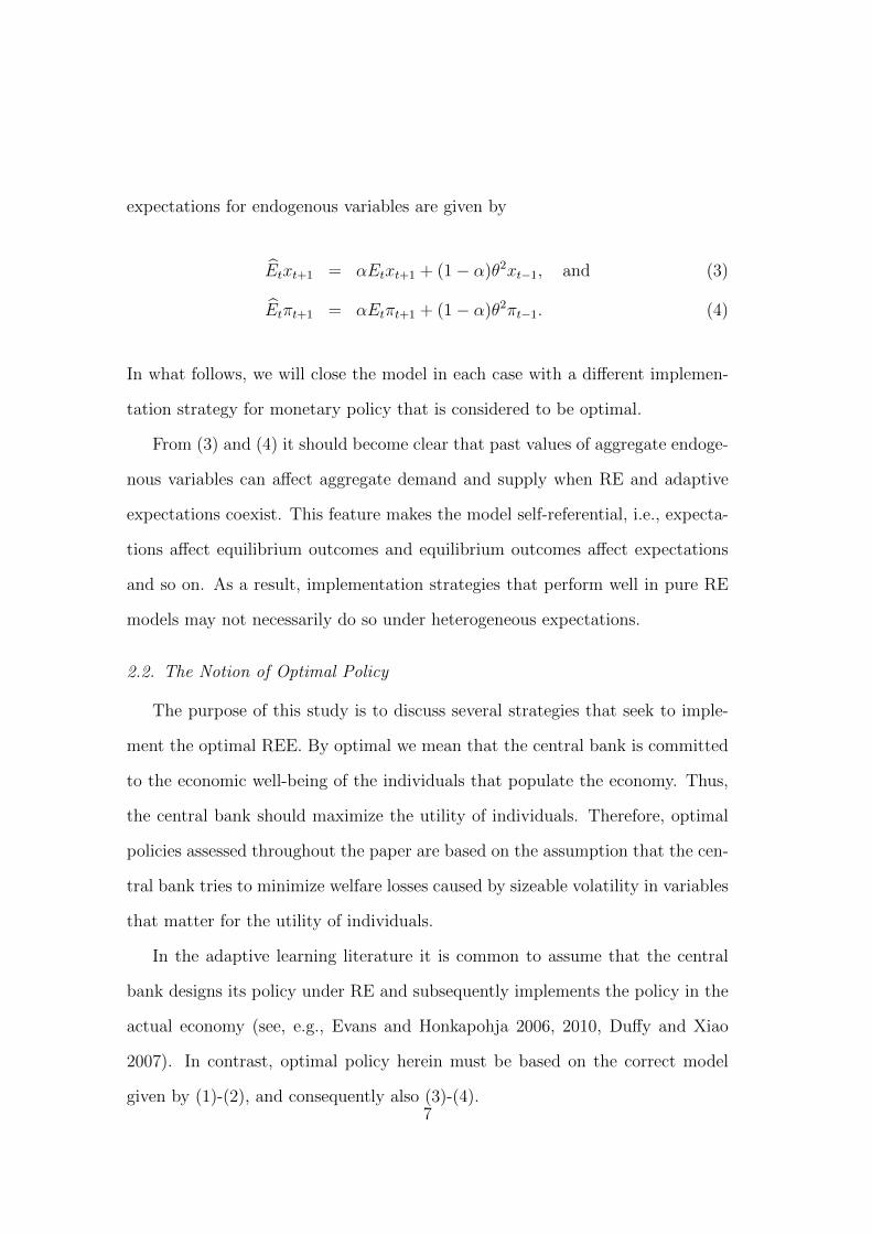
expectations for endogenous variables are given by
bE
t
x
t+1 = ↵E
t
x
t+1 + (1� ↵)✓2xt�1, and (3)
bE
t
⇡
t+1 = ↵E
t
⇡
t+1 + (1� ↵)✓2⇡t�1. (4)
In what follows, we will close the model in each case with a di↵erent implemen-
tation strategy for monetary policy that is considered to be optimal.
From (3) and (4) it should become clear that past values of aggregate endoge-
nous variables can a↵ect aggregate demand and supply when RE and adaptive
expectations coexist. This feature makes the model self-referential, i.e., expecta-
tions a↵ect equilibrium outcomes and equilibrium outcomes a↵ect expectations
and so on. As a result, implementation strategies that perform well in pure RE
models may not necessarily do so under heterogeneous expectations.
2.2. The Notion of Optimal Policy
The purpose of this study is to discuss several strategies that seek to imple-
ment the optimal REE. By optimal we mean that the central bank is committed
to the economic well-being of the individuals that populate the economy. Thus,
the central bank should maximize the utility of individuals. Therefore, optimal
policies assessed throughout the paper are based on the assumption that the cen-
tral bank tries to minimize welfare losses caused by sizeable volatility in variables
that matter for the utility of individuals.
In the adaptive learning literature it is common to assume that the central
bank designs its policy under RE and subsequently implements the policy in the
actual economy (see, e.g., Evans and Honkapohja 2006, 2010, Du↵y and Xiao
2007). In contrast, optimal policy herein must be based on the correct model
given by (1)-(2), and consequently also (3)-(4).7
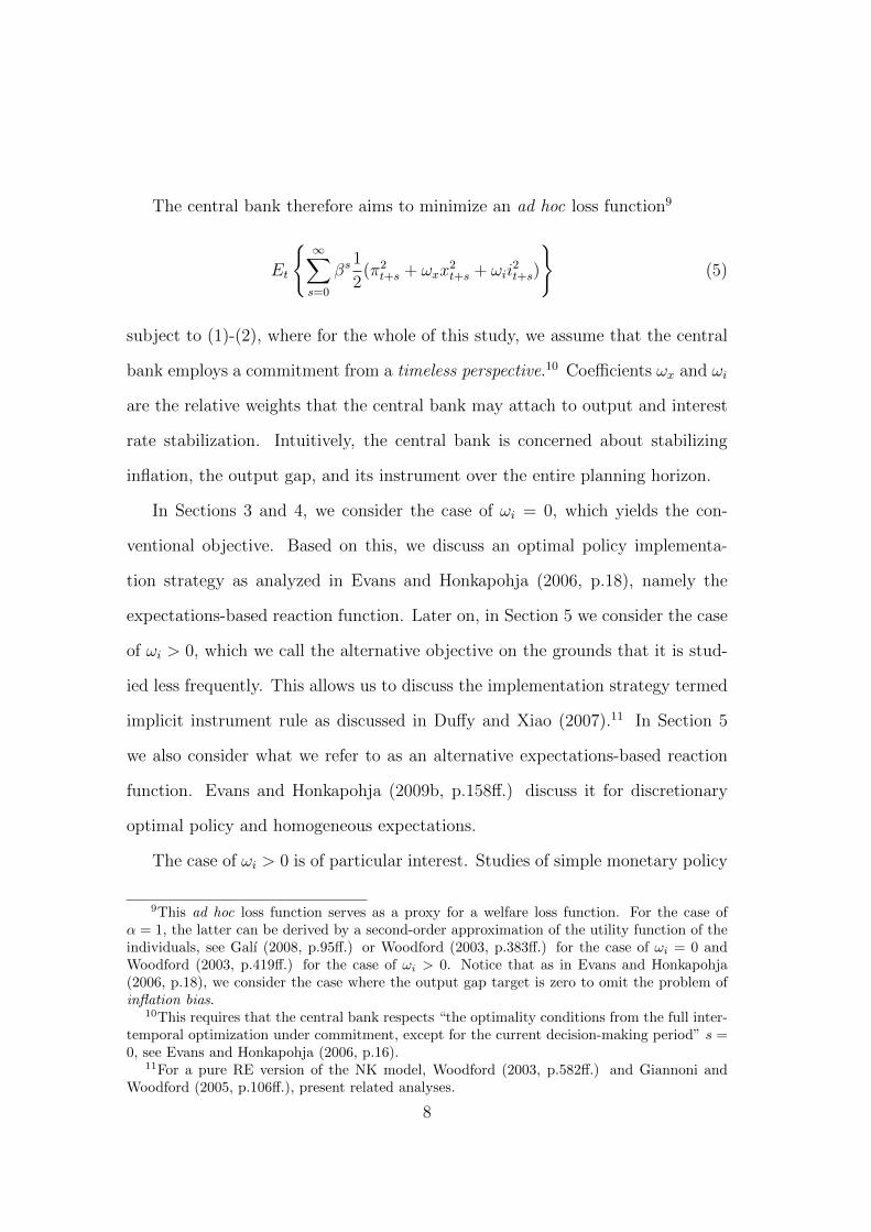
The central bank therefore aims to minimize an ad hoc loss function9
E
t
( 1X
s=0
�
s
1
2(⇡2
t+s
+ !
x
x
2t+s
+ !
i
i
2t+s
)
)(5)
subject to (1)-(2), where for the whole of this study, we assume that the central
bank employs a commitment from a timeless perspective.10 Coe�cients !x
and !
i
are the relative weights that the central bank may attach to output and interest
rate stabilization. Intuitively, the central bank is concerned about stabilizing
inflation, the output gap, and its instrument over the entire planning horizon.
In Sections 3 and 4, we consider the case of !i
= 0, which yields the con-
ventional objective. Based on this, we discuss an optimal policy implementa-
tion strategy as analyzed in Evans and Honkapohja (2006, p.18), namely the
expectations-based reaction function. Later on, in Section 5 we consider the case
of !i
> 0, which we call the alternative objective on the grounds that it is stud-
ied less frequently. This allows us to discuss the implementation strategy termed
implicit instrument rule as discussed in Du↵y and Xiao (2007).11 In Section 5
we also consider what we refer to as an alternative expectations-based reaction
function. Evans and Honkapohja (2009b, p.158↵.) discuss it for discretionary
optimal policy and homogeneous expectations.
The case of !i
> 0 is of particular interest. Studies of simple monetary policy
9This ad hoc loss function serves as a proxy for a welfare loss function. For the case of↵ = 1, the latter can be derived by a second-order approximation of the utility function of theindividuals, see Galı (2008, p.95↵.) or Woodford (2003, p.383↵.) for the case of !
i
= 0 andWoodford (2003, p.419↵.) for the case of !
i
> 0. Notice that as in Evans and Honkapohja(2006, p.18), we consider the case where the output gap target is zero to omit the problem ofinflation bias.
10This requires that the central bank respects “the optimality conditions from the full inter-temporal optimization under commitment, except for the current decision-making period” s =0, see Evans and Honkapohja (2006, p.16).
11For a pure RE version of the NK model, Woodford (2003, p.582↵.) and Giannoni andWoodford (2005, p.106↵.), present related analyses.
8
rules such as Bullard and Mitra (2007) find that policy inertia in simple rules
may be a good tool for avoiding indeterminacy or explosiveness. One might also
wonder, then, whether or not policy inertia has similar e↵ects in the case of
optimal policy. The last term in (5) captures the idea of policy inertia in the
context of optimal monetary policy.12
Finally, we stress that our notion of optimal policy must be understood as ad
hoc optimal policy rather than fully optimal policy for two reasons. First, coe�-
cients !x
and !
i
express the preferences of the central bank. In contrast, under
fully optimal policy these two parameters would be a function of the structural
parameters of the economy. Second, fully optimal policy would require consider-
ing an objective derived from an economy with heterogeneous expectations.
3. THE CONVENTIONAL OBJECTIVE
3.1. Implementation via Expectations-Based Reaction Function I
Evans and Honkapohja (2006) illustrate the derivation of an expectations-
based reaction function of optimal policy given !
i
= 0. One of their main results
of the study is that the expectations-based reaction function is the superior imple-
mentation strategy under homogeneous private sector expectations, being formed
either rational or by adaptive learning. Therefore we focus on the expectations-
based reaction function.13
12See Woodford (2003, p.582↵.) and Giannoni and Woodford (2005, p.106↵.) for detailsof two theoretical arguments in favour of such an objective. Briefly, these are non-negligibletransaction frictions as discussed in Friedman (1969) or punishment of potential violations ofthe zero lower bound on the policy instrument.
13Alternatively the central bank may opt for the so-called fundamentals-based reaction func-tion as its implementation strategy. However, its performance with regard to determinacyand stability under learning is poor even under homogeneous expectations, see e.g. Evans andHonkapohja (2003, 2006, 2009a,b).
9
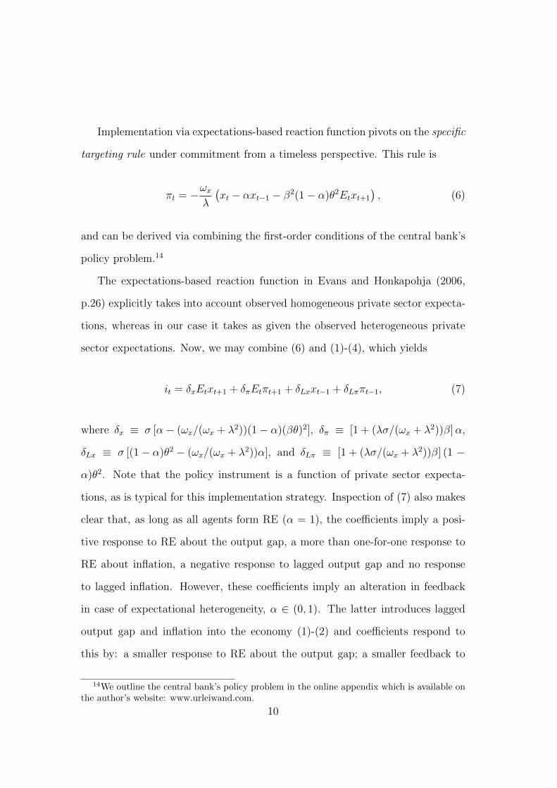
Implementation via expectations-based reaction function pivots on the specific
targeting rule under commitment from a timeless perspective. This rule is
⇡
t
= �!
x
�
�x
t
� ↵x
t�1 � �
2(1� ↵)✓2Et
x
t+1
�, (6)
and can be derived via combining the first-order conditions of the central bank’s
policy problem.14
The expectations-based reaction function in Evans and Honkapohja (2006,
p.26) explicitly takes into account observed homogeneous private sector expecta-
tions, whereas in our case it takes as given the observed heterogeneous private
sector expectations. Now, we may combine (6) and (1)-(4), which yields
i
t
= �
x
E
t
x
t+1 + �
⇡
E
t
⇡
t+1 + �
Lx
x
t�1 + �
L⇡
⇡
t�1, (7)
where �
x
⌘ � [↵� (!x
/(!x
+ �
2))(1� ↵)(�✓)2], �
⇡
⌘ [1 + (��/(!x
+ �
2))�]↵,
�
Lx
⌘ � [(1� ↵)✓2 � (!x
/(!x
+ �
2))↵], and �
L⇡
⌘ [1 + (��/(!x
+ �
2))�] (1 �
↵)✓2. Note that the policy instrument is a function of private sector expecta-
tions, as is typical for this implementation strategy. Inspection of (7) also makes
clear that, as long as all agents form RE (↵ = 1), the coe�cients imply a posi-
tive response to RE about the output gap, a more than one-for-one response to
RE about inflation, a negative response to lagged output gap and no response
to lagged inflation. However, these coe�cients imply an alteration in feedback
in case of expectational heterogeneity, ↵ 2 (0, 1). The latter introduces lagged
output gap and inflation into the economy (1)-(2) and coe�cients respond to
this by: a smaller response to RE about the output gap; a smaller feedback to
14We outline the central bank’s policy problem in the online appendix which is available onthe author’s website: www.urleiwand.com.
10
RE about inflation, eventually less than one-for-one; a larger feedback to lagged
output gap and a positive feedback to lagged inflation. Be aware that policy
potentially violates the form of the Taylor (1993)-principle as discussed in Wood-
ford (2001, p.233), Woodford (2003, p.254), Bullard and Mitra (2002, p.1116),
Bullard and Mitra (2007, p.1183), and Evans and Honkapohja (2009a, p.42),
since (�x
+ �
Lx
)(1� �)/�+ (�⇡
+ �
L⇡
) < 1 is possible for ✓ < 1.
3.2. The Numerical Approach to the Analysis
We base our analysis of reaction functions such as (7) on numerical methods
and illustrate so-called regions of local determinacy, indeterminacy, and explo-
siveness similar to Bullard and Mitra (2002). The di↵erent regions are usually
plotted in a plane where the axes measure either (!x
, ✓) or the monetary pol-
icy parameters (!x
,!
i
) for di↵erent ✓.15 We do so because we are dealing with
high dimensional economic systems that do not provide analytical conditions for
determinacy.
Given a reduced form model (1)-(2) and an implementation strategy, we will
usually end up with a second-order di↵erence system of the form
yt
= AE
t
yt+1 +Cy
t�1, (8)
where yt
is a m ⇥ 1 vector of endogenous variables and matrices A and C are
m ⇥ m matrices. In order to assess the dynamic properties of such a system,
one chooses a solution procedure that, as a by-product, yields the eigenvalues of
the system matrix. It is precisely these eigenvalues that characterize the system
dynamics. One may either apply the solution method of Blanchard and Kahn
15For all cases we provide animated plots for the share of agents with RE, ↵ 2 [0, 1] on theauthor’s website: www.urleiwand.com.
11

(1980) or the more robust purely numerical method proposed by Klein (2000).
The advantage of the latter is that it is based on generalized eigenvalues (GEVs)
and allows matrices A and C to be singular (see McCallum 2009a).
We can thus calculate GEVs for any combination of the monetary policy
parameters. Moreover, we can count the number of GEVs, whose moduli are
inside or outside the unit circle for any parameter combination. In particular,
at any point within the parameter space, where the number of GEVs whose
moduli lie outside the unit circle matches the number of free variables, there is
local determinacy. Next, when the number of GEVs whose moduli lie outside the
unit circle is less than the number of free variables we have local indeterminacy.16
Finally, when the number of GEVs whose moduli lie outside the unit circle exceeds
the number of free variables there is local explosiveness.17
3.3. The Calibration of the Economy
In order to carry out our numerical analysis, we calibrate our model accord-
ing to Table 1. Our choices of �, �, and �, often referred to as the Woodford
(1999)-calibration, allow comparability of our results with the ones of Evans and
Honkapohja (2006) or Du↵y and Xiao (2007) with regard to determinacy.
Furthermore, recall that our analysis considers expectational heterogeneity.
In particular, next to the case of only rational agents, ↵ = 1, we first and fore-
most study the coexistence of rational and non-rational agents, ↵ < 1, which in
turn puts the parameter ✓ into action. This parameter characterizes the type of
16Some authors distinguish indeterminacy of di↵erent order, in which the order measuresthe di↵erence between the number of free variables and the number of GEVs whose modulilie outside the unit circle. For example, when the di↵erence is two, one labels that Order 2Indeterminacy. This denotes a situation with a system exhibiting a two-dimensional continuumof stationary equilibria. The idea behind this is to indicate “the number of independent sunspotsrequired to specify the solution”, see Evans and McGough (2005, p.1816).
17In our analysis we ignore the special case, where one or more moduli of the GEVs may lieon the unit circle.
12
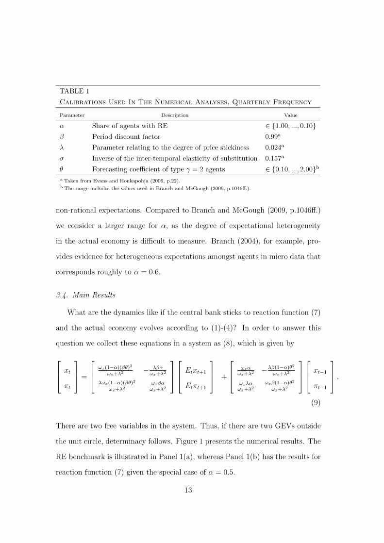
TABLE 1
Calibrations Used In The Numerical Analyses, Quarterly Frequency
Parameter Description Value
↵ Share of agents with RE 2 {1.00, ..., 0.10}� Period discount factor 0.99a
� Parameter relating to the degree of price stickiness 0.024a
� Inverse of the inter-temporal elasticity of substitution 0.157a
✓ Forecasting coe�cient of type � = 2 agents 2 {0.10, ..., 2.00}ba Taken from Evans and Honkapohja (2006, p.22).b The range includes the values used in Branch and McGough (2009, p.1046↵.).
non-rational expectations. Compared to Branch and McGough (2009, p.1046↵.)
we consider a larger range for ↵, as the degree of expectational heterogeneity
in the actual economy is di�cult to measure. Branch (2004), for example, pro-
vides evidence for heterogeneous expectations amongst agents in micro data that
corresponds roughly to ↵ = 0.6.
3.4. Main Results
What are the dynamics like if the central bank sticks to reaction function (7)
and the actual economy evolves according to (1)-(4)? In order to answer this
question we collect these equations in a system as (8), which is given by
2
64x
t
⇡
t
3
75 =
2
64!
x
(1�↵)(�✓)2
!
x
+�
2 � ��↵
!
x
+�
2
�!
x
(1�↵)(�✓)2
!
x
+�
2!
x
�↵
!
x
+�
2
3
75
2
64E
t
x
t+1
E
t
⇡
t+1
3
75 +
2
64!
x
↵
!
x
+�
2 ���(1�↵)✓2
!
x
+�
2
!
x
�↵
!
x
+�
2!
x
�(1�↵)✓2
!
x
+�
2
3
75
2
64x
t�1
⇡
t�1
3
75 .
(9)
There are two free variables in the system. Thus, if there are two GEVs outside
the unit circle, determinacy follows. Figure 1 presents the numerical results. The
RE benchmark is illustrated in Panel 1(a), whereas Panel 1(b) has the results for
reaction function (7) given the special case of ↵ = 0.5.
13
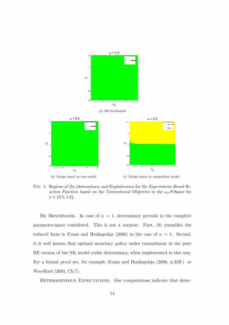
(a) RE benchmark
(b) Design based on true model (c) Design based on misspecified model
Fig. 1. Regions of (In-)determinacy and Explosiveness for the Expectations-Based Re-action Function based on the Conventional Objective in the !
x
-✓-Space for↵ 2 {0.5, 1.0}.
Re Benchmark. In case of ↵ = 1, determinacy prevails in the complete
parameter-space considered. This is not a surprise. First, (9) resembles the
reduced form in Evans and Honkapohja (2006) in the case of ↵ = 1. Second,
it is well known that optimal monetary policy under commitment in the pure
RE version of the NK model yields determinacy, when implemented in this way.
For a formal proof see, for example, Evans and Honkapohja (2006, p.35↵.) or
Woodford (2003, Ch.7).
Heterogeneous Expectations. Our computations indicate that deter-
14
minacy prevails throughout the considered parameter space. Consequently the
optimal policy rule under heterogeneous expectations implements the optimal
REE and successfully rules out suboptimal stationary REE. This extends the
strong result of Evans and Honkapohja (2006) regarding the expectations-based
reaction function as the superior implementation strategy to a heterogeneous ex-
pectations economy. Likewise this finding suggests a resolution to the threats to
economic stability emerging from expectational heterogeneity under simple inter-
est rate rules, as discussed in Branch and McGough (2009) or Massaro (2013).
The intuition for this result is related to the properties of rule (7), as discussed
in Subsection 3.1 above. Consider coe�cients �
⇡
and �
L⇡
, which stipulate the
feedback to RE about inflation and lagged inflation respectively. The size of
�
⇡
(�L⇡
) is negatively (positively) related to ↵. This implies that, as RE about
inflation become less pervasive in the economy, the feedback to RE about inflation
(lagged inflation) gets smaller (larger). In other words, the policy instrument
responds stronger to the type of forecasts that are more relevant to inflation
pressures, either directly via (2) or indirectly via the real interest rate in (1). A
similar line of reasoning applies with regard to �
x
and �
Lx
. Note that xt
directly
a↵ects ⇡
t
in this economy. Again, it
responds stronger to the forecasts of xt
,
which are more relevant to the determination of xt
and in turn to ⇡
t
.
4. ROBUSTNESS TO MISSPECIFICATION IN POLICY DESIGN
Herein we assume that the central bank bases optimal policy design on a mis-
specified RE version of the Phillips curve (2). That is, the central bank aims to
implement the rule that would be optimal if all agents had rational expectations.
One can verify that the design parallels the one in Section 3. Essentially, this
assumption corresponds to ↵ = 1 in (6). As far as the implementation is con-
15
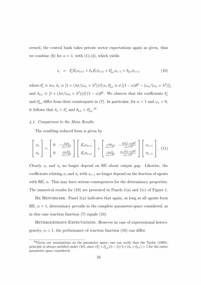
cerned, the central bank takes private sector expectations again as given, thus
we combine (6) for ↵ = 1, with (1)-(4), which yields
i
t
= �
⇤x
E
t
x
t+1 + �
⇡
E
t
⇡
t+1 + �
⇤Lx
x
t�1 + �
L⇡
⇡
t�1, (10)
where �⇤x
⌘ �↵, �⇡
⌘ [1 + (��/(!x
+ �
2))�]↵, �⇤Lx
⌘ � [(1� ↵)✓2 � (!x
/(!x
+ �
2))],
and �
L⇡
⌘ [1 + (��/(!x
+ �
2))�] (1 � ↵)✓2. We observe that the coe�cients �
⇤x
and �
⇤Lx
di↵er from their counterparts in (7). In particular, for ↵ < 1 and !
x
> 0,
it follows that �x
< �
⇤x
and �
Lx
> �
⇤Lx
.18
4.1. Comparison to the Main Results
The resulting reduced form is given by
2
64x
t
⇡
t
3
75 =
2
640 � ��↵
!
x
+�
2
0 !
x
�↵
!
x
+�
2
3
75
2
64E
t
x
t+1
E
t
⇡
t+1
3
75+
2
64!
x
!
x
+�
2 ���(1�↵)✓2
!
x
+�
2
!
x
�
!
x
+�
2!
x
�(1�↵)✓2
!
x
+�
2
3
75
2
64x
t�1
⇡
t�1
3
75 . (11)
Clearly x
t
and ⇡
t
no longer depend on RE about output gap. Likewise, the
coe�cients relating xt
and ⇡
t
with x
t�1 no longer depend on the fraction of agents
with RE, ↵. This may have serious consequences for the determinacy properties.
The numerical results for (10) are presented in Panels 1(a) and 1(c) of Figure 1.
Re Benchmark. Panel 1(a) indicates that again, as long as all agents form
RE, ↵ = 1, determinacy prevails in the complete parameter-space considered, as
in this case reaction function (7) equals (10).
Heterogeneous Expectations. However in case of expectational hetero-
geneity, ↵ < 1, the performance of reaction function (10) can di↵er.
18Given our assumptions on the parameter space, one can verify that the Taylor (1993)-principle is always satisfied under (10), since (�⇤
x
+ �⇤Lx
)(1��)/�+(�⇡
+ �L⇡
) > 1 for the entireparameter space considered.
16
Purely adaptive or naıve expectations. Given that non-rational forecasts are
formed purely adaptively or naıvely, ✓ 1, we observe a qualitatively similar
pattern. The central bank can still render the economy determinate regardless
of its preference within !
x
2 (0, 2]. Thus, conditional on this particular ex-
pectational set-up, our main result even holds under policy design based on a
misspecified model. In addition, our finding is also consistent with the result of
Evans and Honkapohja (2006), in which the reaction function (10) yields stabil-
ity under adaptive learning as with decreasing ↵, average expectations become
purely adaptive.
Extrapolative expectations. Somewhat worrisome is our finding for the case in
which non-rational forecasts are extrapolative, ✓ 2 (1.0, 2.0]. It appears that the
central bank can trigger local explosiveness for many values of !x
.
Variations of ↵ indicate that, for su�ciently large ✓ > 1, the larger the share of
non-rational forecasts, the lower the policy preference !x
must be for determinacy.
Otherwise, optimal policy under RE fails to deliver determinacy. Implicitly this
means that the larger the relative weight on inflation stabilization, the greater is
the chance to ensure determinacy. This finding is consistent with Orphanides and
Williams’s (2005) result, that policy should respond more aggressively towards
inflation in the presence of heterogeneous information.
However, for ↵ 2 {0.1, ..., 0.5} our results suggest that, contrary to the case of
homogeneous RE studied in Evans and Honkapohja (2006), the central bank can
no longer render the economy determinate for a certain part of the parameter
space. The presence of extrapolative expectations is a threat to determinacy
regardless of !
x
. The coe�cients in reaction function (10) and the resulting
reduced form (11) can provide some intuition for this observation. The presence
of non-rational agents, ↵ < 1, induces some di↵erences compared to the case of
17
↵ = 1 and, equally important, to our main results reported above.
First, notice that extrapolative expectations, in contrast to purely adaptive
or naıve expectations, possess the inherent tendency to reinforce cumulative pro-
cesses away from the REE. Now, as ↵ gets smaller, these tendencies in the econ-
omy become stronger. Thus, one may expect a stronger response of the policy
instrument to such tendencies in order to contain the economy in the REE. As
coe�cients �⇡
and �
L⇡
are as in (7), only the central banks stance regarding the
output gap, �x
< �
⇤x
and �
Lx
> �
⇤Lx
, can explain the discrepancy in results.
Second, starting with (1), as ↵ gets smaller, extrapolative expectations re-
garding the output gap get more relevant for the determination of xt
. If there is
an upward pressure in extrapolative expectations of the output gap, xt
tend to
increase, and via (2), ⇡t
does so too. This will feed into expectations of inflation,
which in turn tend to lower the real interest rate in (1) and increase ⇡
t
via (2).
This, in turn, reinforces the mechanism just described.
Third, optimal monetary policy that renders the economy determinate for
given preference !
x
, manages to shut down the mechanism just described, by
responding su�ciently to the relevant expectations. However, in the current case,
despite extrapolative expectations becoming more relevant with smaller ↵, the
feedback to these expectations implied by �⇤Lx
is insu�cient and lower compared to
the one implied by �
Lx
. Thus, under (7), the impact of extrapolative expectations
on x
t
is successfully mitigated, whereas this is not the case under (10).
Finally, note that the relative strength of the mechanism discussed above
also depends on the coe�cient �, which is negatively related to the degree of
nominal price rigidity and governs the sensitivity of inflation to changes in the
output gap. One can show that the smaller is �, i.e., the more sticky nominal
prices are, the more likely it is that the optimal policy rule under RE fails to
18
deliver determinacy given the policymaker’s preference !
x
> 0 throughout the
whole range ✓ 2 [0.1, 2.0], as ↵ decreases. This finding suggests that, in order to
achieve determinacy in this scenario, the central bank may be required to act as
if it would favour a lower weight on output gap stabilization, as it actually does.
Overall, our results for the expectations-based reaction function (10) suggest
that in an NK economy with heterogeneous expectations the central bank is
unable to control nominal prices throughout the parameter space. This pitfall
puts a warning sign on this implementation strategy and contrasts with the Evans
and Honkapohja (2006, 2010) result for homogeneous expectations and our main
results above, obtained for policy design in the correctly specified model.
4.2. Discussion19
Based on the findings within this section, one may argue that, as long as
non-rational expectations are purely adaptive, the policymaker can ignore expec-
tational heterogeneity in the policy design. However, such a behaviour of the
central bank raises the issue of time-consistency: the policy rule designed under
the misspecified or approximating model will de facto never be satisfied, as the
expectational heterogeneity is persistent.20 Thus, can the policymaker credibly
commit to such a policy rule? Or, wouldn’t one expect that the policymaker
would deviate and instead change the policy design?21
19I owe particular thanks to an anonymous referee for his thoughtful suggestions that formthe basis of this discussion.
20This distinguishes the set-up herein from Evans and Honkapohja (2006), where the optimalpolicy rule designed in the RE version of the economy is implemented asymptotically as privatesector expectations asymptotically converge to RE.
21Such concerns are consistent with the literature, which assumes that the policymakerinitially possesses a misspecified model, but may uncover the true model over time via least-squares learning. However, it is routinely assumed that the policymaker’s misspecification isunintended and turns out to be transient. Such scenarios are elaborated in Sargent (1999,p.68↵.) for optimal policy and in Carlstrom and Fuerst (2004) for simple interest rate rules. Inthe former case policy turns out to be time-consistent.
19
Clearly, the policymaker can only credibly commit to the design based on the
approximating model, if the actual processes of endogenous variables, resulting
from combining this design with the true model, appear to be equivalent to the
ones that he expects to be generated by the designed policy in combination with
the approximating model. If not equivalent, it is straightforward to ask, why
repeatedly missing the target does not provoke doubts over the policymaker’s
approximating model? The central bank’s doubts about the model could either
manifest themselves in terms of parameters of, or variables included in, its per-
ceived law of motion (PLM).
The question of whether doubts about the policymaker’s model are justified,
can be addressed by asking under which conditions a self-confirming equilibrium,
as outlined in Sargent (1999, p.68↵.), Evans and Honkapohja (2001, p.325↵.)
and Cho, Williams, and Sargent (2002), exists.22 For the purpose of analysis, one
has to elaborate the central bank’s optimal policy design in the approximating
model of the economy, where the doubts are parametrized by some coe�cients.
The design is implemented into this model which results into the PLM. Next,
the policymaker’s optimal policy designed under the approximating model, im-
plemented into the true model, yields the so-called actual law of motion (ALM).
Accordingly, the policymaker can only credibly commit to its optimal policy, if
the ALM is consistent with the PLM.
We have addressed both types of doubts from above.23 Our results suggest
that committing to an optimal policy rule, designed in an economic model which
employs the REH, is time-inconsistent, when the actual economy features per-
22According to Evans and Honkapohja (2001) this is an example of a restricted perceptionsequilibrium. Although, in the special case of a self-confirming equilibrium the misspecificationcan only be uncovered out of equilibrium.
23The analysis is included in the online appendix.
20
sistent expectational heterogeneity. Thus, it cannot be an equilibrium outcome.
This finding asserts that in practice it may not be credible for a central bank to
commit to an optimal policy rule designed within a RE version of a DSGE model.
However, recall that our analysis is conducted in a deterministic set-up. In
contrast, in a stochastic version of the model, it may be possible that the approach
to optimal policy discussed in this section is time-consistent. Assume that the
policymaker utilizes a least-squares learning procedure to estimate the coe�cients
of the PLM. These coe�cients would have to satisfy a least-squares projection
of the true model onto the approximating model. If so, then asymptotically, i.e.,
within a self-confirming equilibrium, the policymaker would not have any reason
to have doubts about the approximating model.24
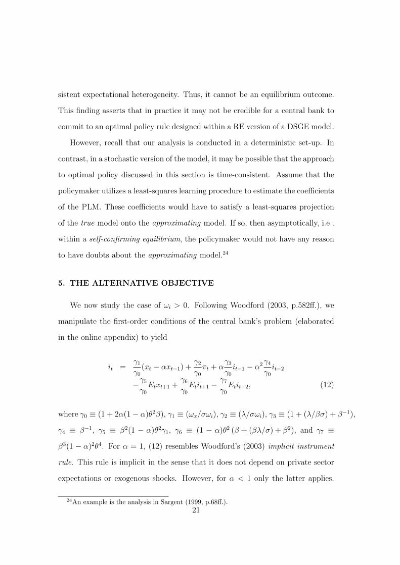
5. THE ALTERNATIVE OBJECTIVE
We now study the case of !i
> 0. Following Woodford (2003, p.582↵.), we
manipulate the first-order conditions of the central bank’s problem (elaborated
in the online appendix) to yield
i
t
=�1
�0
(xt
� ↵x
t�1) +�2
�0
⇡
t
+ ↵
�3
�0
i
t�1 � ↵
2�4
�0
i
t�2
��5
�0
E
t
x
t+1 +�6
�0
E
t
i
t+1 ��7
�0
E
t
i
t+2, (12)
where �0 ⌘ (1 + 2↵(1� ↵)✓2�), �1 ⌘ (!x
/�!
i
), �2 ⌘ (�/�!i
), �3 ⌘ (1 + (�/��) + �
�1),
�4 ⌘ �
�1, �5 ⌘ �
2(1 � ↵)✓2�1, �6 ⌘ (1 � ↵)✓2 (� + (��/�) + �
2), and �7 ⌘
�
3(1 � ↵)2✓4. For ↵ = 1, (12) resembles Woodford’s (2003) implicit instrument
rule. This rule is implicit in the sense that it does not depend on private sector
expectations or exogenous shocks. However, for ↵ < 1 only the latter applies.
24An example is the analysis in Sargent (1999, p.68↵.).21
Furthermore, Woodford (2003) proves that commitment to this rule yields a de-
terminate REE that is optimal from a timeless perspective as long as ↵ = 1.
Moreover, Du↵y and Xiao (2007) examine rule (12) for the case in which homo-
geneous expectations are formed via adaptive learning. They find that it yields
stability under learning for a large fraction of the relevant parameter space. This
motivates our assessment of rule (12) under heterogeneous expectations, as it is
also a possible implementation strategy for the central bank in this scenario.
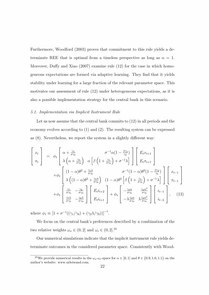
5.1. Implementation via Implicit Instrument Rule
Let us now assume that the central bank commits to (12) in all periods and the
economy evolves according to (1) and (2). The resulting system can be expressed
as (8). Nevertheless, we report the system in a slightly di↵erent way:
2
64x
t
⇡
t
3
75 = �1
2
64↵ + �5
��0�
�1↵(1� ��2
�0)
�
⇣↵ + �5
��0
⌘↵
h�
⇣1 + �1
��0
⌘+ �
�1�
i
3
75
2
64E
t
x
t+1
E
t
⇡
t+1
3
75
+�1
2
64(1� ↵)✓2 + �1↵
��0�
�1(1� ↵)✓2(1� ��2
�0)
�
⇣(1� ↵)✓2 + �1↵
��0
⌘(1� ↵)✓2
h�
⇣1 + �1
��0
⌘+ �
�1�
i
3
75
2
64x
t�1
⇡
t�1
3
75
+�1
2
64�7
��0� �6
��0
�7�
��0��6�
��0
3
75
2
64E
t
i
t+2
E
t
i
t+1
3
75+ �1
2
64��3↵
��0
�4↵2
��0
��
�3↵
��0�
�4↵2
��0
3
75
2
64i
t�1
i
t�2
3
75 , (13)
where �1 ⌘ [1 + �
�1((�1/�0) + (�2�/�0))]�1.
We focus on the central bank’s preferences described by a combination of the
two relative weights !x
2 (0, 2] and !
i
2 (0, 2].25
Our numerical simulations indicate that the implicit instrument rule yields de-
terminate outcomes in the considered parameter space. Consistently with Wood-
25We provide numerical results in the !x
-!i
-space for ↵ 2 [0, 1] and ✓ 2 {0.9, 1.0, 1.1} on theauthor’s website: www.urleiwand.com.
22
ford (2003), this is true for the RE benchmark, ↵ = 1. But the same holds for
the case of heterogeneous expectations, ↵ < 1.
Thus, with regard to determinacy, the implicit instrument rule appears to
have a similar performance compared to that of the expectations-based reaction
function above. Likewise, for the case of ↵ = 1 it is sometimes argued, that rule
(12) is easier to implement, as the central bank does not need to track private
sector expectations. However, this operational advantage over an expectations-
based reaction function vanishes in case of expectational heterogeneity and on the
other hand, the rule requires the central bank to observe contemporaneous values
of ⇡t
and x
t
. Finally, if !i
! 0, then both, �1 ! 1 and �2 ! 1. This is discussed
in Evans and Honkapohja (2009b) and arguably raises additional concerns about
how operational the implicit instrument rule is, and further questions the merit
of policy inertia in this context.
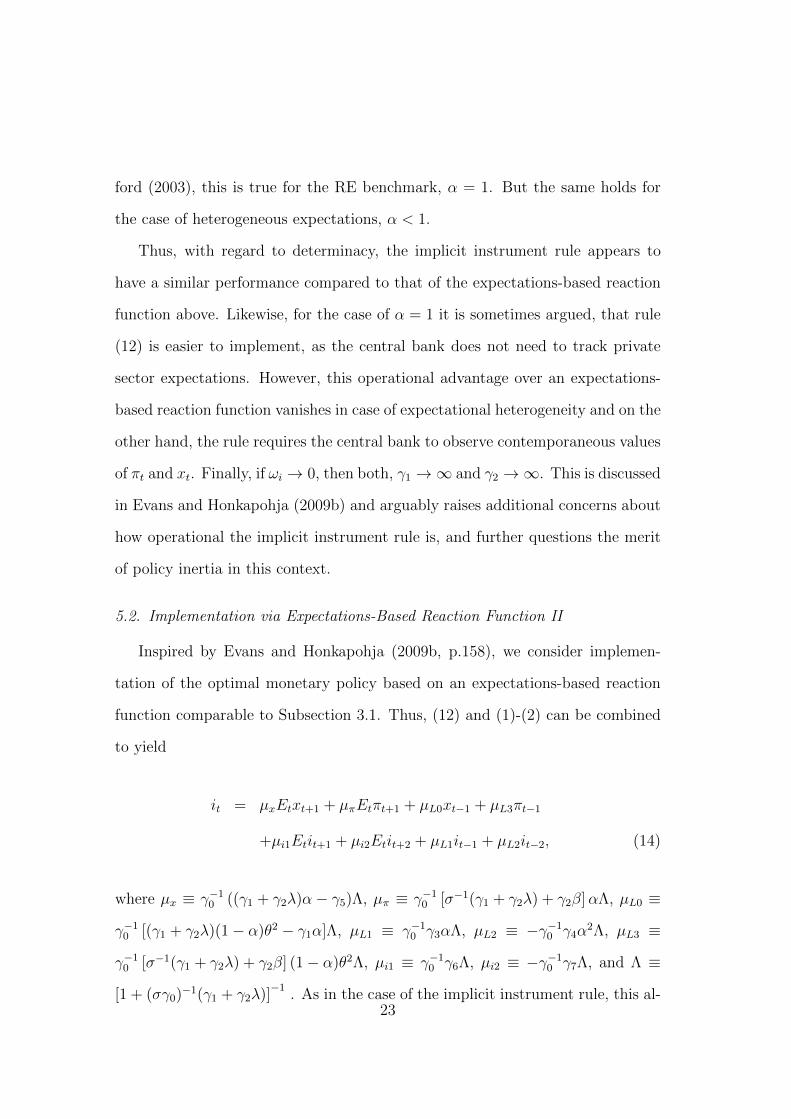
5.2. Implementation via Expectations-Based Reaction Function II
Inspired by Evans and Honkapohja (2009b, p.158), we consider implemen-
tation of the optimal monetary policy based on an expectations-based reaction
function comparable to Subsection 3.1. Thus, (12) and (1)-(2) can be combined
to yield
i
t
= µ
x
E
t
x
t+1 + µ
⇡
E
t
⇡
t+1 + µ
L0xt�1 + µ
L3⇡t�1
+µ
i1Et
i
t+1 + µ
i2Et
i
t+2 + µ
L1it�1 + µ
L2it�2, (14)
where µ
x
⌘ �
�10 ((�1 + �2�)↵� �5)⇤, µ⇡
⌘ �
�10 [��1(�1 + �2�) + �2�]↵⇤, µL0 ⌘
�
�10 [(�1 + �2�)(1� ↵)✓2 � �1↵]⇤, µ
L1 ⌘ �
�10 �3↵⇤, µ
L2 ⌘ ��
�10 �4↵
2⇤, µ
L3 ⌘
�
�10 [��1(�1 + �2�) + �2�] (1� ↵)✓2⇤, µ
i1 ⌘ �
�10 �6⇤, µi2 ⌘ ��
�10 �7⇤, and ⇤ ⌘
[1 + (��0)�1(�1 + �2�)]�1 . As in the case of the implicit instrument rule, this al-
23
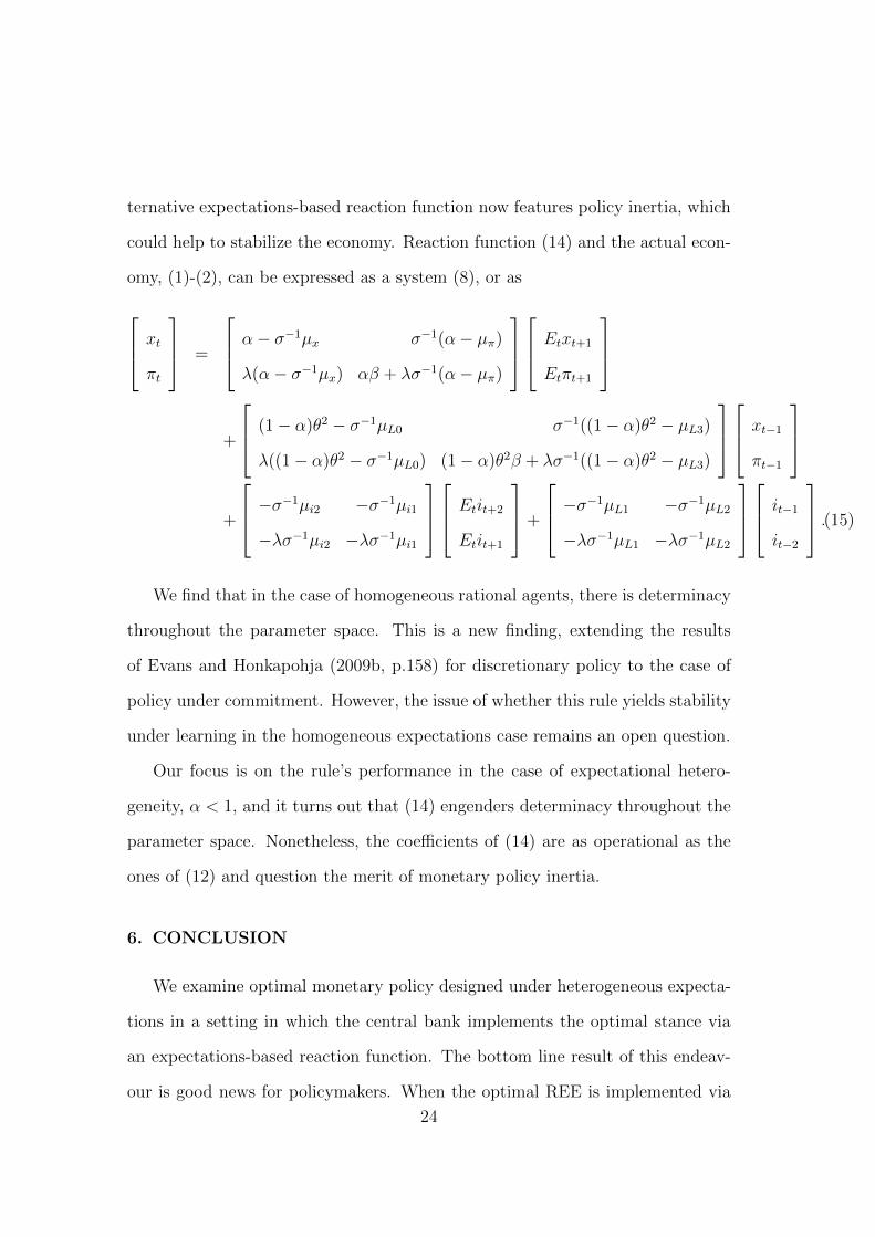
ternative expectations-based reaction function now features policy inertia, which
could help to stabilize the economy. Reaction function (14) and the actual econ-
omy, (1)-(2), can be expressed as a system (8), or as
2
64x
t
⇡
t
3
75 =
2
64↵� �
�1µ
x
�
�1(↵� µ
⇡
)
�(↵� �
�1µ
x
) ↵� + ��
�1(↵� µ
⇡
)
3
75
2
64E
t
x
t+1
E
t
⇡
t+1
3
75
+
2
64(1� ↵)✓2 � �
�1µ
L0 �
�1((1� ↵)✓2 � µ
L3)
�((1� ↵)✓2 � �
�1µ
L0) (1� ↵)✓2� + ��
�1((1� ↵)✓2 � µ
L3)
3
75
2
64x
t�1
⇡
t�1
3
75
+
2
64��
�1µ
i2 ��
�1µ
i1
���
�1µ
i2 ���
�1µ
i1
3
75
2
64E
t
i
t+2
E
t
i
t+1
3
75+
2
64��
�1µ
L1 ��
�1µ
L2
���
�1µ
L1 ���
�1µ
L2
3
75
2
64i
t�1
i
t�2
3
75 .(15)
We find that in the case of homogeneous rational agents, there is determinacy
throughout the parameter space. This is a new finding, extending the results
of Evans and Honkapohja (2009b, p.158) for discretionary policy to the case of
policy under commitment. However, the issue of whether this rule yields stability
under learning in the homogeneous expectations case remains an open question.
Our focus is on the rule’s performance in the case of expectational hetero-
geneity, ↵ < 1, and it turns out that (14) engenders determinacy throughout the
parameter space. Nonetheless, the coe�cients of (14) are as operational as the
ones of (12) and question the merit of monetary policy inertia.
6. CONCLUSION
We examine optimal monetary policy designed under heterogeneous expecta-
tions in a setting in which the central bank implements the optimal stance via
an expectations-based reaction function. The bottom line result of this endeav-
our is good news for policymakers. When the optimal REE is implemented via
24
an expectations-based reaction function, which appropriately takes into account
heterogeneous private-sector expectations, local determinacy prevails. Thus, our
main result implies that central banks can successfully rule out suboptimal equi-
libria in an economy with heterogeneous expectations and are able to fully shield
the economy against locally explosive paths and arbitrary large fluctuations.
Next we take up an issue of practical relevance. Can a central bank design
optimal monetary policy based on a misspecified model, implement it via an
expectations-based reaction function, and still rule out suboptimal REE? The
answer is: it depends. It works, if non-rational agents form purely adaptive or
naıve expectations. However, if these agents form extrapolative expectations, the
central bank runs the risk of losing control over inflation and output in the pres-
ence of expectational heterogeneity. In any case, we find that such a policy is not
time-consistent. This insight furthers the key implication of our main result that
in a world with heterogeneous expectations, the central bank should incorporate
expectational heterogeneity into the design of optimal monetary policy.
Subsequently we analyze optimal monetary policy when the central bank’s
objective enforces policy inertia. We examine two implementation strategies, the
implicit instrument rule and an alternative expectations-based reaction function.
We find that both implementation strategies can render the economy determinate
for the parameter space considered.
However, the implementation strategies raise serious concerns regarding their
practical value for the conduct of monetary policy, as they are not operational in
the presence of heterogeneous expectations. Thus, the merit of policy inertia is
far from evident and clear-cut policy recommendations are elusive.
Put di↵erently, these shortcomings call for a new approach to designing opti-
mal policy when interest-rate stabilization is involved, that can better deal with
25
the potential hazards of expectational heterogeneity. In this setting the question
of the merit of policy inertia could then be restated and reexamined.
REFERENCES
Assenza, Tiziana, Peter Heemeijer, Cars H. Hommes, and Domenico Massaro. (2013) “Individ-
ual Expectations and Aggregate Macro Behavior.” Tinbergen Institute Discussion Paper 16,
Tinbergen Institute.
Blanchard, Olivier J., and Charles M. Kahn. (1980) “The Solution of Linear Di↵erence Models
under Rational Expectations.” Econometrica, 48, 1305–1311.
Branch, William A. (2004) “The Theory of Rationally Heterogeneous Expectations: Evidence
from Survey Data on Inflation Expectations.” Economic Journal, 114, 592–621.
Branch, William A., and George W. Evans. (2011) “Monetary Policy and Heterogeneous Ex-
pectations.” Economic Theory, 47, 365–393.
Branch, William A., and Bruce McGough. (2009) “A New Keynesian Model with Heterogeneous
Expectations.” Journal of Economic Dynamics and Control, 33, 1036–1051.
Bullard, James B., and Kaushik Mitra. (2002) “Learning about Monetary Policy Rules.” Jour-
nal of Monetary Economics, 49, 1105–1129.
Bullard, James B., and Kaushik Mitra. (2007) “Determinacy, Learnability, and Monetary Policy
Inertia.” Journal of Money, Credit and Banking, 39, 1177–1212.
Carlstrom, Charles T., and Timothy S. Fuerst. (2004) “Learning and the Central Bank.” Journal
of Monetary Economics, 51, 327–338.
Cho, In-Koo, Noah Williams, and Thomas J. Sargent. (2002) “Escaping Nash Inflation.” Review
of Economic Studies, 69, 1–40.
Christiano, Lawrence J., Mathias Trabandt, and Karl Walentin. (2010) “DSGEModels for Mon-
etary Policy Analysis.” In Handbook of Monetary Economics, Vol. 3, edited by Benjamin M.
Friedman, and Michael Woodford, pp. 285–367, Amsterdam: North Holland.
Clarida, Richard H., Jordi Galı, and Mark Gertler. (1999) “The Science of Monetary Policy: A
New Keynesian Perspective.” Journal of Economic Literature, 37, 1661–1707.
Cochrane, John H. (2009) “Can Learnability Save New-Keynesian Models?” Journal of Mon-
etary Economics, 56, 1109–1113.
26
Cochrane, John H. (2011) “Determinacy and Identification with Taylor Rules.” Journal of
Political Economy, 119, 565–615.
Du↵y, John, and Wei Xiao. (2007) “The Value of Interest Rate Stabilization Policies When
Agents Are Learning.” Journal of Money, Credit and Banking, 39, 2041–2056.
Evans, George W., and Seppo Honkapohja. (2001) Learning and Expectations in Macroeco-
nomics. Frontiers of Economic Research, Princeton, NJ: Princeton University Press.
Evans, George W., and Seppo Honkapohja. (2003) “Expectations and the Stability Problem
for Optimal Monetary Policies.” Review of Economic Studies, 70, 807–824.
Evans, George W., and Seppo Honkapohja. (2006) “Monetary Policy, Expectations and Com-
mitment.” Scandinavian Journal of Economics, 108, 15–38.
Evans, George W., and Seppo Honkapohja. (2009a) “Expectations, Learning and Monetary
Policy: An Overview of Recent Research.” InMonetary Policy Under Uncertainty and Learn-
ing, Series on Central Banking, Analysis, and Economic Policies, Vol. XIII, edited by Klaus
Schmidt-Hebbel, and Carl E. Walsh, pp. 27–76, Santiago, Chile: Central Bank of Chile.
Evans, George W., and Seppo Honkapohja. (2009b) “Robust Learning Stability with Opera-
tional Monetary Policy Rules.” In Monetary Policy Under Uncertainty and Learning, Series
on Central Banking, Analysis, and Economic Policies, Vol. XIII, edited by Klaus Schmidt-
Hebbel, and Carl E. Walsh, pp. 145–170, Santiago, Chile: Central Bank of Chile.
Evans, George W., and Seppo Honkapohja. (2010) “Corrigendum: Monetary Policy, Expecta-
tions and Commitment.” Scandinavian Journal of Economics, 112, 640–641.
Evans, George W., and Bruce McGough. (2005) “Monetary Policy, Indeterminacy and Learn-
ing.” Journal of Economic Dynamics and Control, 29, 1809–1840.
Friedman, Milton. (1969) “The Optimum Quantity of Money.” In The Optimum Quantity of
Money and Other Essays, pp. 1–50, Chicago: Aldine.
Galı, Jordi. (2008) Monetary Policy, Inflation, and the Business Cycle: An Introduction to the
New Keynesian Framework. Princeton, NJ: Princeton University Press.
Giannoni, Marc P., and Michael Woodford. (2005) “Optimal Inflation-Targeting Rules.” In The
Inflation-Targeting Debate, Studies in Business Cycles, Vol. 32, edited by Ben S. Bernanke,
and Michael Woodford, pp. 93–162, Chicago and London: The University of Chicago Press.
Klein, Paul. (2000) “Using the Generalized Schur Form to Solve a Multivariate Linear Rational
Expectations Model.” Journal of Economic Dynamics and Control, 24, 1405–1423.
27
Kydland, Finn E., and Edward C. Prescott. (1977) “Rules Rather than Discretion: The Incon-
sistency of Optimal Plans.” Journal of Political Economy, 85, 473–491.
Massaro, Domenico. (2013) “Heterogeneous Expectations in Monetary DSGE Models.” Journal
of Economic Dynamics and Control, 37, 680–692.
McCallum, Bennett T. (2009a) “Causality, Structure, and the Uniqueness of Rational Expec-
tations Equilibria.” The Manchester School, 79, 551–566.
McCallum, Bennett T. (2009b) “Inflation Determination with Taylor Rules: Is New Keynesian
Analysis Critically Flawed?” Journal of Monetary Economics, 56, 1101–1108.
McCallum, Bennett T. (2009c) “Rejoinder to Cochrane.” Journal of Monetary Economics, 56,
1114–1115.
Orphanides, Athanasios, and John C. Williams. (2005) “Imperfect Knowledge, Inflation Ex-
pectations, and Monetary Policy.” In The Inflation-Targeting Debate, Studies in Business
Cycles, Vol. 32, edited by Ben S. Bernanke, and Michael Woodford, pp. 201–234, Chicago
and London: The University of Chicago Press.
Sargent, Thomas J. (1999) The Conquest of American Inflation. Princeton, NJ: Princeton
University Press.
Smets, Frank, and Rafael Wouters. (2003) “An Estimated Dynamic Stochastic General Equilib-
rium Model of the Euro Area.” Journal of the European Economic Association, 1, 1207–1238.
Smets, Frank, and Rafael Wouters. (2007) “Shocks and Frictions in US Business Cycles: A
Bayesian DSGE Approach.” American Economic Review, 97, 586–606.
Taylor, John B. (1993) “Discretion versus Policy Rules in Practice.” Carnegie-Rochester Con-
ference Series on Public Policy, 39, 195–214.
Woodford, Michael. (1999) “Optimal Monetary Policy Inertia.” NBER Working Paper 7261,
National Bureau of Economic Research.
Woodford, Michael. (2001) “The Taylor Rule and Optimal Monetary Policy.” American Eco-
nomic Review, 91, 232–237.
Woodford, Michael. (2003) Interest and Prices: Foundations of a Theory of Monetary Policy.
Princeton, NJ: Princeton University Press.
28