Heterogeneous Production Efficiency of Specialized Swine Producers

Glynn T. Tonsor (gtonsor@agecon.ksu.edu)

and

Allen M. Featherstone (afeather@agecon.ksu.edu)

Kansas State University Manhattan, KS

Selected working paper prepared for presentation at the Southern Agricultural Economics Association Annual Meetings

Orlando, Florida, February 5-8, 2006

Copyright 2006 by Glynn T. Tonsor and Allen M. Featherstone. All rights reserved. Readers may make verbatim copies of this document for non-commercial purposes by any means, provided that this copyright notice appears on all such copies.

Heterogeneous Production Efficiency of Specialized Swine Producers

Abstract

This research evaluates the efficiency of swine firms differing by specialization type and

employed technologies. Measures of technical, allocative, scale, economic, and overall

efficiency are separately and jointly estimated for farrow-to-finish, farrow-to-feeder, feeder-to-

finish, farrow-to-weanling, weanling-to-feeder, and mixed operations. Findings confirm

appreciable differences in efficiency and causes of efficiency. Results suggest that overall

efficiency of farrow-to-finish and farrow-to-weanling operations is on average lower than

farrow-to-feeder, feeder-to-finish, and weanling-to-feeder operations. In addition, Tobit models

examining how demographic factors, farm type, and input expenses influence efficiency indicate

additional variation across firm specializations. This information can help aid in making more

appropriate decisions such as producers altering their input mixes or researchers evaluating the

existence and implications of firm heterogeneity in an industry.

Key words: efficiency, heteroskedastic Tobit, firm specialization, future anticipation, producer

heterogeneity, production technology, returns to scale, swine

Introduction

The swine industry in the US, like much of the agricultural sector in general, has been

changing drastically in recent years. Between 1994 and 1999, the number of swine operations

fell by over 50% (McBride and Key). The proportion of total market hogs produced from

traditional farrow-to-finish operations fell from approximately 65% to less than 38% between

1992 and 1998. This change was coupled with an increase in production by specialized hog

operations (as a percentage of total US production) from 22% to 58% (McBride and Key). In

addition to changes in production specialization, there are significant locational changes

occurring in the industry. Onal, Unnevehr, and Bekric note industry trends for larger, more

efficient operations to be shifting from the Midwest to the Southeast. With rapid adjustment

throughout the industry comes increased pressure for firms to become more efficient to simply

remain in the industry. Two principle questions that arise from these observations are “How

does business performance vary among different specialized swine production operations?” and

“What factors most impact performance of these specialized firms?” While the implications of

these issues are significant for swine producers, policy makers, and others, to our knowledge

they have not previously been evaluated in the literature and warrant further investigation.

Research on efficiency of swine producers is in itself limited and has focused on several

different issues. Rowland et al. examined input use efficiency for 43 farrow-to-finish operators

in Kansas for three sequential years. They found that inefficient farms tend to remain inefficient

over time and that there is more variability in technical and allocative efficiency over time than

in scale efficiency. In addition, they found overall efficient firms typically produced more pork

per litter, fed a higher percentage of their own feed grains, and had lower debt-to-asset ratios.

1

Boland and Patrick analyzed the economic performance for 60 pork producers (primarily

farrow-to-finish operators) across 21 quarters spanning from 1986 to 1991. Feed efficiency and

pigs sold per sow had the largest impacts on returns. Consistent with Rowland et al., they found

that producer’s performance relative to competition tends to be stable over time. Sharma, Leung,

and Zalenski compared the use of output-oriented DEA models and stochastic frontier

production functions in analyzing technical efficiency of 60 swine producers in Hawaii. They

found DEA derived efficiency estimates to be lower and attribute this occurrence to the DEA

approach attributing all deviations from the frontier to inefficiency. The authors proceed to

suggest that production could be increased by 25-40% if producers operated on the efficient

frontier.

Each of these prior studies used regional data with a rather small sample of producers,

which may not be representative of the US swine production industry as a whole. In addition,

understanding how firm efficiency varies across different swine operation types is a crucial

element in accurately comprehending why rapid change is occurring in the swine industry and

why firms in various segments of the industry are experiencing mixed business success. Most

previous research has not considered the heterogeneity of operation types that exist in the

industry. In a sense, this reduces the ability to capture differences that likely exists due to

differences in production specialization and employed technologies. This paper seeks to shed

light on this by explicitly incorporating organizational structure in an examination of how

various swine producing firms operate in their aim to become efficient and survive the recent

period of rapid adjustment. Furthermore, this analysis provides an examination of how different

operator demographics, size, and firm specialization impact efficiency. In particular, an

2

evaluation of how the number of additional years an operator anticipates producing is provided

that has not been previously considered in the literature.

More specifically, technical, allocative, scale, economic, and overall efficiency estimates

are developed in this study for different swine production specializations. The firm types

considered are “farrow-to-finish,” “farrow-to-feeder,” “feeder-to-finish,” “farrow-to-weanling,”

“weanling-to-feeder,” and “mixed” operations. Furthermore, estimated Tobit models examining

factors related to efficiency measures are used to identify factors that are heterogeneous across

firms and across organizational structures.

Methods: Firm Efficiency Estimation

Production efficiency has traditionally been examined by either parametric or

nonparametric approaches. The parametric approach involves selecting a functional form and

estimating the deviation of data observations from the suggested functional form. The

nonparametric technique does not require the selection of an underlying functional form. This

approach makes relative comparisons with firms within a particular dataset. The nonparametric

approach is chosen for this paper and follows that of Banker, Charnes, and Cooper and Färe,

Grosskopf, and Lovell.

Relative measures of technical, allocative, scale, economic, and overall efficiency are

derived for each individual firm for each different production specialization. To accomplish this,

separate linear programming problems are solved for every farm.

Technical Efficiency

Technical efficiency is defined as the ability of a firm to either produce the highest level

of output with a set input bundle and technology or to produce the current level of output with

3

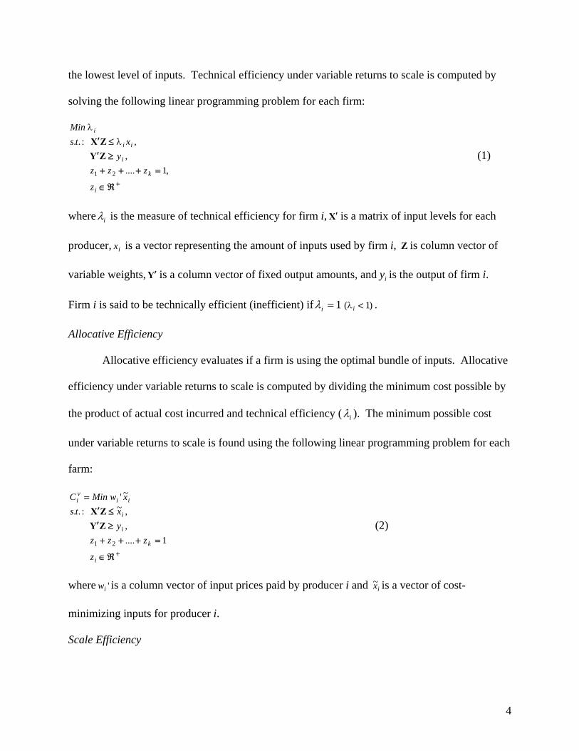
the lowest level of inputs. Technical efficiency under variable returns to scale is computed by

solving the following linear programming problem for each firm:

+ℜ∈

=+++≥′≤′

i

k

i

ii

i

z

zzzy

xtsMin

,1....,

,:..

21

ZYZX λ

λ

(1)

where iλ is the measure of technical efficiency for firm i, X′ is a matrix of input levels for each

producer, is a vector representing the amount of inputs used by firm i, is column vector of

variable weights, Y is a column vector of fixed output amounts, and is the output of firm i.

Firm i is said to be technically efficient (inefficient) if

ix Z

′ iy

1=iλ )1( <iλ .

Allocative Efficiency

Allocative efficiency evaluates if a firm is using the optimal bundle of inputs. Allocative

efficiency under variable returns to scale is computed by dividing the minimum cost possible by

the product of actual cost incurred and technical efficiency ( iλ ). The minimum possible cost

under variable returns to scale is found using the following linear programming problem for each

farm:

+ℜ∈

=+++≥′≤′

=

i

k

i

i

iivi

z

zzzyxts

xwMinC

1....,,~:..

~'

21

ZYZX

(2)

where is a column vector of input prices paid by producer i and 'iw ix~ is a vector of cost-

minimizing inputs for producer i.

Scale Efficiency

4

Scale efficiency compares a firm’s current operational size with what is most efficient in

terms of minimizing average cost. Scale efficiency is calculated as the ratio of minimum

possible cost under constant returns to scale ( ) to the minimum cost feasible under variable

returns to scale ( ). is found using linear programming problem labeled above as (2)

without imposing the constraint on the sum of variable weights.

ciC

viC c

iC

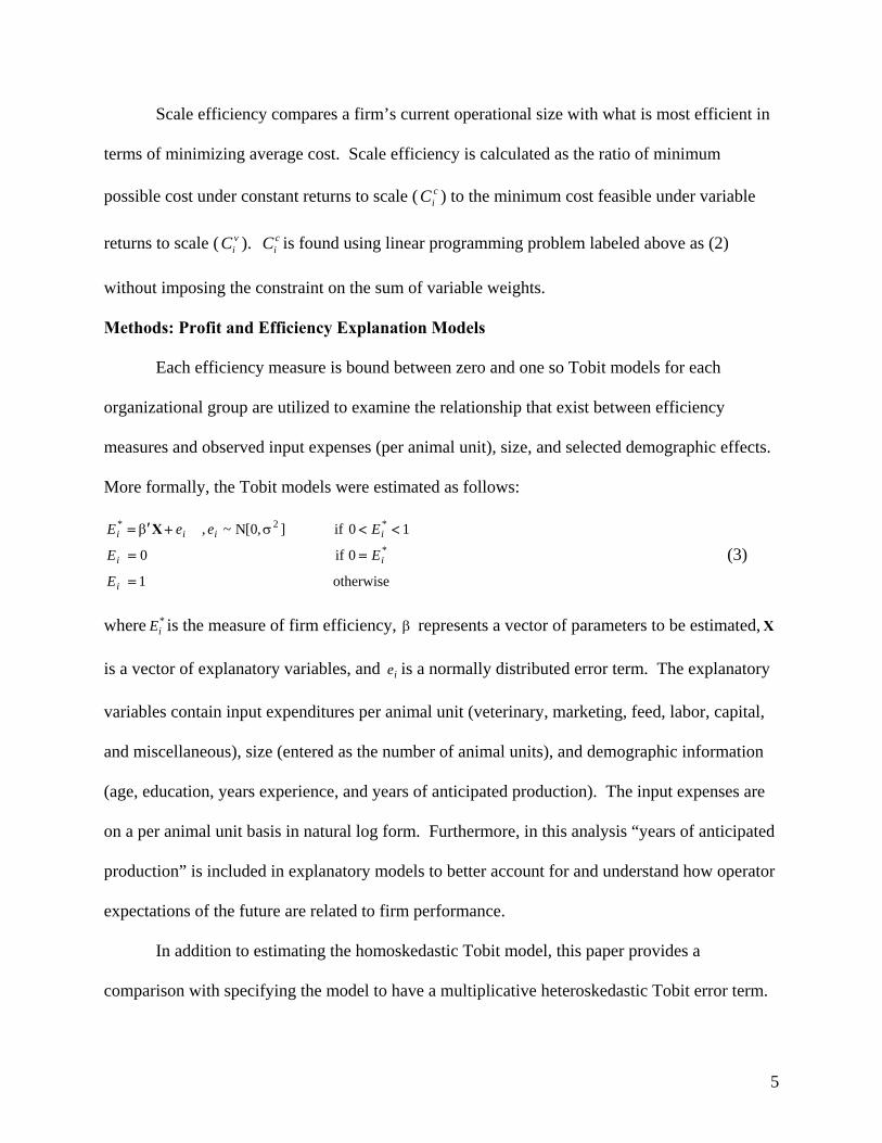
Methods: Profit and Efficiency Explanation Models

Each efficiency measure is bound between zero and one so Tobit models for each

organizational group are utilized to examine the relationship that exist between efficiency

measures and observed input expenses (per animal unit), size, and selected demographic effects.

More formally, the Tobit models were estimated as follows:

otherwise1

0if0

10if],0[N~,*

*2*

=

==

<<+′=

i

ii

iiii

E

EE

EeeE σβ X

(3)

where is the measure of firm efficiency, *iE β represents a vector of parameters to be estimated,

is a vector of explanatory variables, and is a normally distributed error term. The explanatory

variables contain input expenditures per animal unit (veterinary, marketing, feed, labor, capital,

and miscellaneous), size (entered as the number of animal units), and demographic information

(age, education, years experience, and years of anticipated production). The input expenses are

on a per animal unit basis in natural log form. Furthermore, in this analysis “years of anticipated

production” is included in explanatory models to better account for and understand how operator

expectations of the future are related to firm performance.

X

ie

In addition to estimating the homoskedastic Tobit model, this paper provides a

comparison with specifying the model to have a multiplicative heteroskedastic Tobit error term.

5

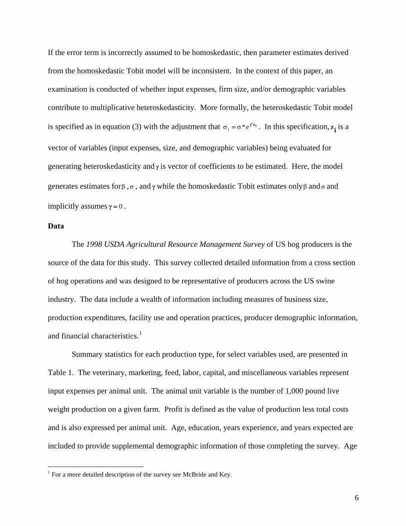
If the error term is incorrectly assumed to be homoskedastic, then parameter estimates derived

from the homoskedastic Tobit model will be inconsistent. In the context of this paper, an

examination is conducted of whether input expenses, firm size, and/or demographic variables

contribute to multiplicative heteroskedasticity. More formally, the heteroskedastic Tobit model

is specified as in equation (3) with the adjustment that izγ′= ei *σσ . In this specification, is a

vector of variables (input expenses, size, and demographic variables) being evaluated for

generating heteroskedasticity and is vector of coefficients to be estimated. Here, the model

generates estimates for

iz

γ

β , , and while the homoskedastic Tobit estimates only andσ and

implicitly assumes .

σ γ β

0=γ

Data

The 1998 USDA Agricultural Resource Management Survey of US hog producers is the

source of the data for this study. This survey collected detailed information from a cross section

of hog operations and was designed to be representative of producers across the US swine

industry. The data include a wealth of information including measures of business size,

production expenditures, facility use and operation practices, producer demographic information,

and financial characteristics.1

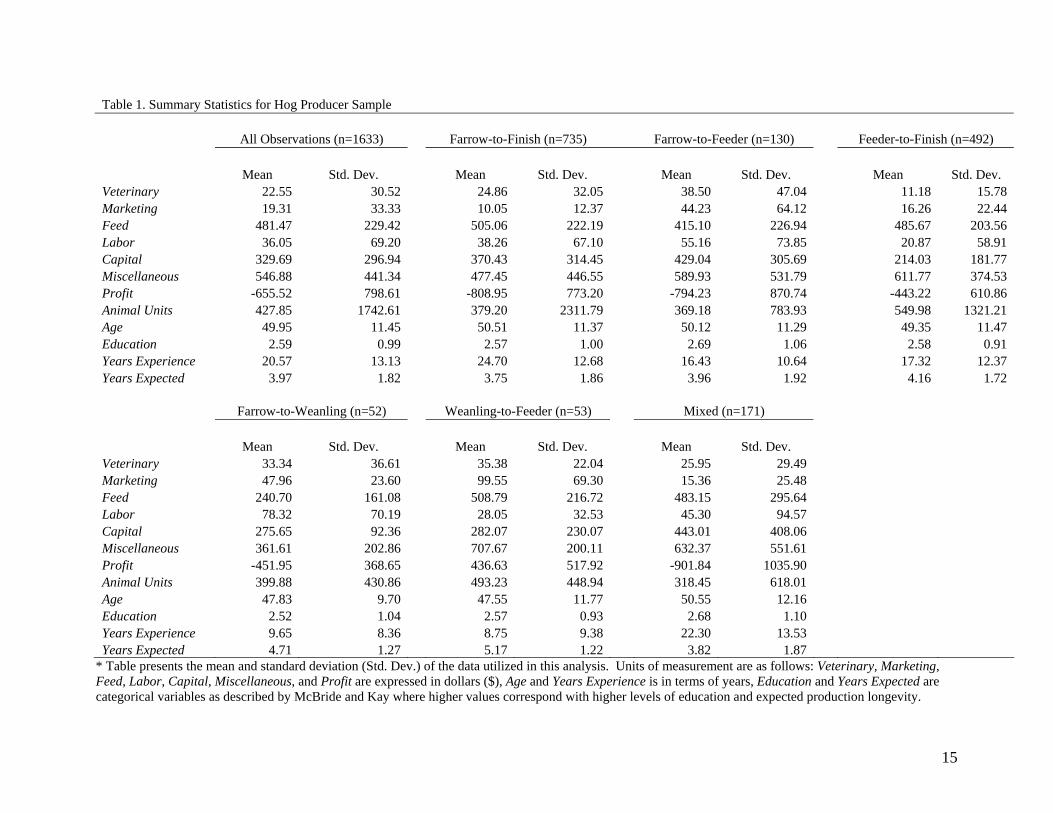
Summary statistics for each production type, for select variables used, are presented in

Table 1. The veterinary, marketing, feed, labor, capital, and miscellaneous variables represent

input expenses per animal unit. The animal unit variable is the number of 1,000 pound live

weight production on a given farm. Profit is defined as the value of production less total costs

and is also expressed per animal unit. Age, education, years experience, and years expected are

included to provide supplemental demographic information of those completing the survey. Age

1 For a more detailed description of the survey see McBride and Key.

6

and education represent the individual’s age (years) and education level. Years experience is a

variable capturing the number of years the underlying operation has been producing hogs.

Similarly, the years expected variable symbolizes the number of years the operator expects the

operation to continue producing hogs.

Examining the summary statistics presented in Table 1 we observe that the typical

producer completing the 1998 USDA Agricultural Resource Management Survey was about 50

years old. While the average age is fairly consistent across firm specialization types, profit, size,

education, experience, and planned years of production all vary appreciably. These differences

may lead to differences in efficiency and causes of efficiency. To further evaluate if a

comparison of efficiency across farm specialization is justified, profit was regressed across firm

specialization, input expenses, and demographic factors. As shown in Table 2, farrow-to-

weanling operations are the only specialization not found to differ significantly at the 10% level

(ceteris paribus) from mixed operations in terms of farm profit.2 Furthermore, the underlying

technology used differs considerably across specializations. Between the noted differences in

firm summary statistics, the results of the profit regression, and observed use of heterogeneous

technology, it appears that further analysis of efficiency measures across specialization is

warranted.

Results

Efficiency Estimates

Table 3 provides a summary of the relative efficiency measures estimated for the entire

dataset (1,633 firms) and for each of the 6 subsets representing the different organizational

structures.3 Technical efficiency (TE) averaged 0.66 for the group as a whole with a standard

2 Mixed operations were omitted (and are the base for comparison) to avoid multicollinearity. 3 Efficiency estimates for each specialization type were estimated with separate frontiers for each specialization.

7

deviation of 0.25. This implies that on average, input use could be reduced by 34% if all

operations were producing on the frontier. Approximately 19% of the firms (as a whole) were

estimated as technically efficient. When comparing this with individual group results,

heterogeneity in efficiency estimates becomes evident. For example, the average farrow-to-

finish and mixed producers are less efficient (with mean estimates of 0.59 and 0.60, respectively)

and the average weanling-to-feeder and farrow-to-feeder operators are notably more efficient

(with mean estimates of 0.88 and 0.83, respectively) than those in other specialization categories.

The range in mean estimates from 0.59 (farrow-to-finish) to 0.88 (weanling-to-feeder) sheds

light on the importance in analyzing firm efficiency based on underlying technologies and not

simply considering the swine industry as being homogeneous.

Allocative efficiency (AE) averaged 0.80 for the entire set of firms, with 21% being

estimated as efficient. Allocative efficiency was highest (on average) for feeder-to-finish

operations which held a mean efficiency estimate of 0.90 (31% estimated as efficient).

Conversely, the representative producer in the mixed group had an allocative efficiency estimate

of 0.69 (18% being efficient). Scale efficiency (SE) averaged 0.88 across all 1,633 firms (with

43% being estimated as efficient) and had means for subset groups ranging from 0.85 (farrow-to-

feeder) to 0.97 (weanling-to-feeder). The mean scale efficiency was higher than mean economic

efficiency for each specialization group. This implies that failing to produce at the optimal scale

is less of an efficiency issue than failing to produce on the cost frontier. This, combined with the

fact that scale efficiency was higher (on average) for each specialization group than technical and

allocative efficiency, suggests that swine producers of all specializations would generally benefit

by focusing more on producing on the frontier than on adjusting size.

8

Economic efficiency (EE) had a mean estimate of 0.53 across all firms and ranged (on

average) from 0.42 (mixed producers) to 0.78 (weanling-to-feeder operators).4 This range across

operations is notably higher than the individual range of technical, allocative, or scale efficiency.

Overall efficiency (OE) averaged 0.48 for the entire data set, with 7% of the sample

being estimated as overall efficient.5 Average overall efficiency ranged across segmented

groups from 0.38 (farrow-to-finish and mixed) to 0.76 (weanling-to-feeder). As noted in the

economic efficiency discussion above, this range is significant. Figure 1 further demonstrates

how overall efficiency varies across farm type. The graph demonstrates significant variation in

the distributions across specialization. For example, it shows that only 15% of weanling-to-

feeder producers are less than 50% efficient compared to 80% of farrow-to-finish operators.

In addition to estimating scale efficiency, returns to scale and optimal size were analyzed.

Table 4 presents the results revealing that returns to scale vary considerably across firm

specialization. Farrow-to-finish and farrow-to-feeder operations were estimated to be the two

groups who could most benefit by increasing operation size as they were found to have the

highest percentage of firms currently operating under increasing returns to scale. Conversely,

80% or more of the feeder-to-finish, farrow-to-weanling, and weanling-to-feeder operations were

estimated to be working under decreasing returns to scale (on the increasing portion of the

average cost curve). Overall, the finding of high scale efficiency (Table 3) and decreasing

returns to scale for the majority of firms implies that the average cost curve is relatively flat

(Rowland et al.). The optimal size of firms (as defined by minimizing average costs) in each

specialization group is presented in table 5.

Tobit Model Results

4 Economic efficiency is defined as the product of technical and allocative efficiency. 5 Overall efficiency is defined as the product of technical, allocative, and scale efficiency.

9

Likelihood ratio tests were used (Table 6) to identify whether the homoskedastic or

heteroskedastic model specifications were more appropriate.6 In all 35 models (7 data subsets

and 5 different efficiency measures) the tests suggests that the heteroskedastic error specification

is statistically more appropriate. Failing to acknowledge this and simply using the traditional

homoskedastic Tobit model may lead to inconsistent parameter estimates. The estimation results

for the heteroskedastic Tobit specifications are presented in table 7.

Analysis of the results reveals that input expenses, firm size, and demographic variables

have mixed effects on each of the five efficiency measures for the different farm specializations.

Furthermore, the heteroskedastic parameters vary considerably across models. With the

exception of the models explaining scale efficiency, the estimated models generally reveal an

inverse relationship between input expenses and firm efficiency. It is noteworthy that this does

not hold in all cases and that the exceptions (e.g., positive impact of marketing expenses on

allocative efficiency for farrow-to-finish and feeder-to-finish farms and the positive influence on

overall efficiency of increased feed expenditures for farrow-to-weanling operators) should be

noted and appreciated by producers, policy makers, and researchers.

Further examination of Table 7 reveals differences in how firm size impacts efficiency

for each of the specializations. It is noteworthy that firm size had a positive and statistically

significant impact (except for in the weanling-to-feeder group) in each of the overall efficiency

models. This finding should be noted by individuals interested in farm size issues related to

market power concerns as this analysis suggests that there are in fact efficiency gains to

increasing firm size. It is interesting to note that farrow-to-finish operations are the only firms in

which farm size has a significant impact on technical efficiency. This implies that the ability of

6 See Table 6 for test statistic calculation formula.

10

most swine farms to produce on the production frontier is not actually impacted by operation

size.

Examination of demographic effects demonstrates heterogeneous impacts on firms

depending on their specialization. In general, age is estimated to have little impact on each

efficiency measure. One notable exception to this is the fact that all five efficiency measures for

farrow-to-weanling firms are significantly affected by age. Operator education and experience

were found to have differing impacts on efficiency depending on firm specialization. Higher

levels of education were found (ceteris paribus) to decrease overall efficiency of farrow-to-

finish, farrow-to-weanling, and weanling-to-feeder farms. Conversely, more experience is

estimated to increase overall efficiency for these same specializations. The number of years a

producer anticipates to continue production appears to be positively related to overall efficiency

of farrow-to-finish and weanling-to-feeder operations and negatively related for farrow-to-

weanling producers. This finding may reflect a tendency of individuals who intend to remain in

the industry for longer periods to adopt newer, more efficient practices than those who are likely

to exit the industry and thus have a shorter time period to justify additional investments in new

technologies.

Conclusions

Previous research on the efficiency of swine firms has been unable to study the effect of

different technologies used in the rapidly changing swine industry. This work is particularly

unique as it provides estimates of technical, allocative, scale, economic, and overall efficiency

separately and jointly for “farrow-to-finish,” “farrow-to-feeder,” “feeder-to-finish,” “farrow-to-

weanling,” “weanling-to-feeder,” and “mixed” operations. Heteroskedastic Tobit models are

11

estimated to examine factors affecting efficiency measures and document heterogeneous impacts

across organizational structures.

Efficiency measures differ appreciably across swine firm specialization. Significant

differences in efficiency estimates are found to persist for firms in each of the analyzed

specialization fields. Estimated Tobit models reveal that heterogeneity extends beyond

specialization type and into the effect of various factors on efficiency estimates. In particular,

input expenses, firm size, and demographic effects are found to have varying impacts on the

evaluated efficiency measures. Furthermore, this analysis provides evidence that the optimal

farm size varies significantly depending on the technology being employed.

The findings of this work have several important implications. This work shows that

firms of differing specializations vary notably in their levels of efficiency and in the underlying

factors influencing this efficiency. Furthermore, this research sheds light on the different

impacts input expenses, operation size, demographic factors, and production technologies have

on estimates of firm efficiency. Future work should take note of these differences across firm

specialization by segmenting firms by the underlying technologies being used (when possible)

and better noting the limitations of assuming firms to have the same technology when it is not

feasible to segment groups by employed technologies.

There are numerous economic implications and contributions from this analysis. These

include demonstrating the impact of incorrectly assuming technology homogeneity when

heterogeneity persists, showing the different effects that demographic factors can have on firm

efficiency, and providing additional evidence that increases in firm size are at least partially

justified by gains in overall production efficiency. Policy makers and operators can better

appreciate these facts and consequently make more informed and appropriate decisions for each

12

specialization type. For instance, policy makers concerned with issues such as firm size can use

this work as a guide in noting that firm size can be motivated by firms seeking to improve

efficiency and that these factors differ substantially across firm specialization. Producers can

utilize this work in several ways; such as guiding adjustment in their input mix to become more

efficient or in considering growth such as moving from a farrow-to-feeder to a farrow-to-finish

operation. Furthermore, researchers can take note of these issues and extend this work in many

ways. For example, one could evaluate the extent and implications of producer heterogeneity in

other industries, account for demographic factors such as producer expectations regarding the

future, as well as provide a further examination of the swine industry using alternative data sets

or modeling techniques.

13

14

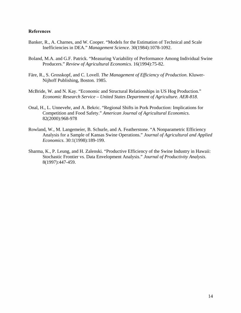
References

Banker, R., A. Charnes, and W. Cooper. “Models for the Estimation of Technical and Scale Inefficiencies in DEA.” Management Science. 30(1984):1078-1092.

Boland, M.A. and G.F. Patrick. “Measuring Variability of Performance Among Individual Swine

Producers.” Review of Agricultural Economics. 16(1994):75-82. Färe, R., S. Grosskopf, and C. Lovell. The Management of Efficiency of Production. Kluwer-

Nijhoff Publishing, Boston. 1985. McBride, W. and N. Kay. “Economic and Structural Relationships in US Hog Production.”

Economic Research Service – United States Department of Agriculture. AER-818. Onal, H., L. Unnevehr, and A. Bekric. “Regional Shifts in Pork Production: Implications for

Competition and Food Safety.” American Journal of Agricultural Economics. 82(2000):968-978

Rowland, W., M. Langemeier, B. Schurle, and A. Featherstone. “A Nonparametric Efficiency

Analysis for a Sample of Kansas Swine Operations.” Journal of Agricultural and Applied Economics. 30:1(1998):189-199.

Sharma, K., P. Leung, and H. Zalenski. “Productive Efficiency of the Swine Industry in Hawaii:

Stochastic Frontier vs. Data Envelopment Analysis.” Journal of Productivity Analysis. 8(1997):447-459.

15

Table 1. Summary Statistics for Hog Producer Sample All Observations (n=1633) Farrow-to-Finish (n=735) Farrow-to-Feeder (n=130) Feeder-to-Finish (n=492) Mean Std. Dev. Mean Std. Dev. Mean Std. Dev. Mean Std. Dev. Veterinary 22.55 30.52 24.86 32.05 38.50 47.04 11.18 15.78 Marketing 19.31 33.33 10.05 12.37 44.23 64.12 16.26 22.44 Feed 481.47 229.42 505.06 222.19 415.10 226.94 485.67 203.56 Labor 36.05 69.20 38.26 67.10 55.16 73.85 20.87 58.91 Capital 329.69 296.94 370.43 314.45 429.04 305.69 214.03 181.77 Miscellaneous 546.88 441.34 477.45 446.55 589.93 531.79 611.77 374.53 Profit -655.52 798.61 -808.95 773.20 -794.23 870.74 -443.22 610.86 Animal Units 427.85 1742.61 379.20 2311.79 369.18 783.93 549.98 1321.21 Age 49.95 11.45 50.51 11.37 50.12 11.29 49.35 11.47 Education 2.59 0.99 2.57 1.00 2.69 1.06 2.58 0.91 Years Experience 20.57 13.13 24.70 12.68 16.43 10.64 17.32 12.37 Years Expected 3.97 1.82 3.75 1.86 3.96 1.92 4.16 1.72 Farrow-to-Weanling (n=52) Weanling-to-Feeder (n=53) Mixed (n=171) Mean Std. Dev. Mean Std. Dev. Mean Std. Dev. Veterinary 33.34 36.61 35.38 22.04 25.95 29.49 Marketing 47.96 23.60 99.55 69.30 15.36 25.48 Feed 240.70 161.08 508.79 216.72 483.15 295.64 Labor 78.32 70.19 28.05 32.53 45.30 94.57 Capital 275.65 92.36 282.07 230.07 443.01 408.06 Miscellaneous 361.61 202.86 707.67 200.11 632.37 551.61 Profit -451.95 368.65 436.63 517.92 -901.84 1035.90 Animal Units 399.88 430.86 493.23 448.94 318.45 618.01 Age 47.83 9.70 47.55 11.77 50.55 12.16 Education 2.52 1.04 2.57 0.93 2.68 1.10 Years Experience 9.65 8.36 8.75 9.38 22.30 13.53 Years Expected 4.71 1.27 5.17 1.22 3.82 1.87

* Table presents the mean and standard deviation (Std. Dev.) of the data utilized in this analysis. Units of measurement are as follows: Veterinary, Marketing, Feed, Labor, Capital, Miscellaneous, and Profit are expressed in dollars ($), Age and Years Experience is in terms of years, Education and Years Expected are categorical variables as described by McBride and Kay where higher values correspond with higher levels of education and expected production longevity.

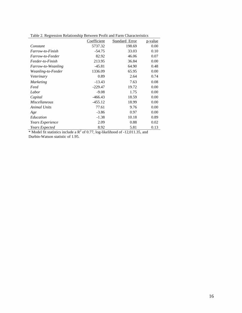
Table 2. Regression Relationship Between Profit and Farm Characteristics Coefficient Standard Error p-valueConstant 5737.32 198.69 0.00 Farrow-to-Finish -54.75 33.03 0.10 Farrow-to-Feeder 82.92 46.06 0.07 Feeder-to-Finish 213.95 36.84 0.00 Farrow-to-Weanling -45.81 64.90 0.48 Weanling-to-Feeder 1336.09 65.95 0.00 Veterinary 0.89 2.64 0.74 Marketing -13.43 7.63 0.08 Feed -229.47 19.72 0.00 Labor -9.08 1.75 0.00 Capital -466.43 18.59 0.00 Miscellaneous -455.12 18.99 0.00 Animal Units 77.61 9.76 0.00 Age -3.86 0.97 0.00 Education -1.38 10.18 0.89 Years Experience 2.09 0.88 0.02 Years Expected 8.92 5.81 0.13

* Model fit statistics include a R2 of 0.77, log-likelihood of -12,011.35, and Durbin-Watson statistic of 1.95.

16

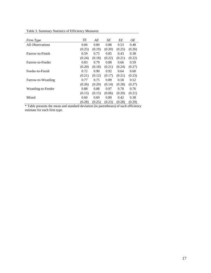
Table 3. Summary Statistics of Efficiency Measures Firm Type TE AE SE EE OE All Observations 0.66 0.80 0.88 0.53 0.48 (0.25) (0.19) (0.20) (0.25) (0.26) Farrow-to-Finish 0.59 0.75 0.85 0.43 0.38 (0.24) (0.18) (0.22) (0.21) (0.22) Farrow-to-Feeder 0.83 0.79 0.88 0.66 0.59 (0.20) (0.18) (0.21) (0.24) (0.27) Feeder-to-Finish 0.72 0.90 0.92 0.64 0.60 (0.21) (0.12) (0.17) (0.21) (0.23) Farrow-to-Weanling 0.77 0.75 0.89 0.58 0.52 (0.26) (0.20) (0.14) (0.28) (0.27) Weanling-to-Feeder 0.88 0.88 0.97 0.78 0.76 (0.15) (0.15) (0.06) (0.20) (0.21) Mixed 0.60 0.69 0.89 0.42 0.38 (0.28) (0.25) (0.23) (0.28) (0.29)

* Table presents the mean and standard deviation (in parentheses) of each efficiency estimate for each firm type.

17

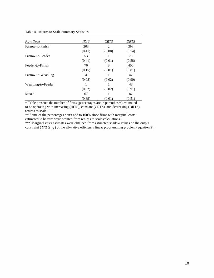
Table 4. Returns to Scale Summary Statistics Firm Type IRTS CRTS DRTS Farrow-to-Finish 303 2 398 (0.41) (0.00) (0.54) Farrow-to-Feeder 53 1 75 (0.41) (0.01) (0.58) Feeder-to-Finish 76 3 400 (0.15) (0.01) (0.81) Farrow-to-Weanling 4 1 47 (0.08) (0.02) (0.90) Weanling-to-Feeder 1 1 48 (0.02) (0.02) (0.91) Mixed 67 1 87 (0.39) (0.01) (0.51) * Table presents the number of firms (percentages are in parentheses) estimated to be operating with increasing (IRTS), constant (CRTS), and decreasing (DRTS) returns to scale. ** Some of the percentages don’t add to 100% since firms with marginal costs estimated to be zero were omitted from returns to scale calculations. *** Marginal costs estimates were obtained from estimated shadow values on the output constraint ( ) of the allocative efficiency linear programming problem (equation 2). iy≥′ZY

18

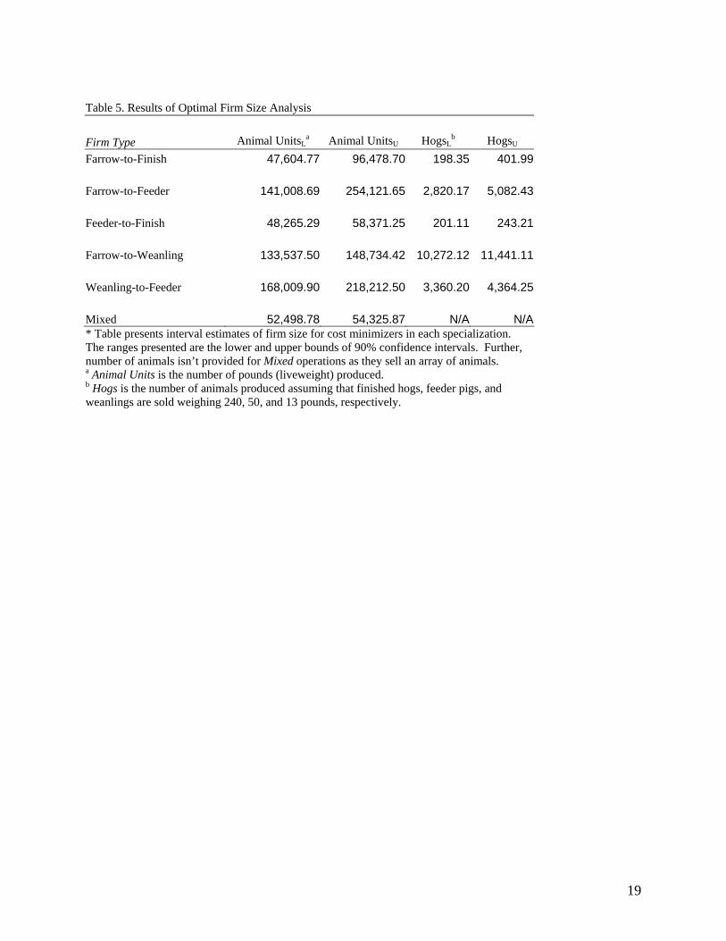
Table 5. Results of Optimal Firm Size Analysis Firm Type Animal UnitsL

a Animal UnitsU HogsLb HogsU

Farrow-to-Finish 47,604.77 96,478.70 198.35 401.99 Farrow-to-Feeder 141,008.69 254,121.65 2,820.17 5,082.43 Feeder-to-Finish 48,265.29 58,371.25 201.11 243.21 Farrow-to-Weanling 133,537.50 148,734.42 10,272.12 11,441.11 Weanling-to-Feeder 168,009.90 218,212.50 3,360.20 4,364.25 Mixed 52,498.78 54,325.87 N/A N/A * Table presents interval estimates of firm size for cost minimizers in each specialization. The ranges presented are the lower and upper bounds of 90% confidence intervals. Further, number of animals isn’t provided for Mixed operations as they sell an array of animals. a Animal Units is the number of pounds (liveweight) produced. b Hogs is the number of animals produced assuming that finished hogs, feeder pigs, and weanlings are sold weighing 240, 50, and 13 pounds, respectively.

19

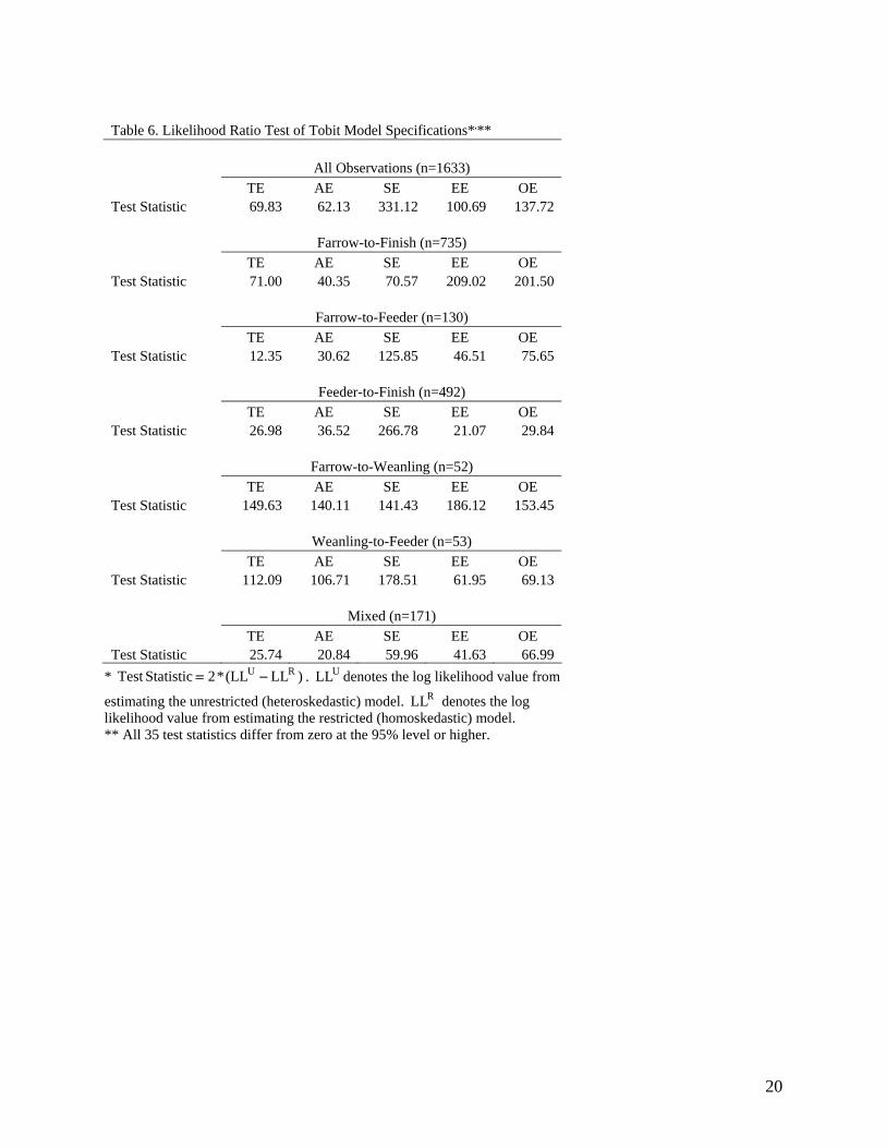
Table 6. Likelihood Ratio Test of Tobit Model Specifications*,**

All Observations (n=1633) TE AE SE EE OE Test Statistic 69.83 62.13 331.12 100.69 137.72

Farrow-to-Finish (n=735) TE AE SE EE OE Test Statistic 71.00 40.35 70.57 209.02 201.50

Farrow-to-Feeder (n=130) TE AE SE EE OE Test Statistic 12.35 30.62 125.85 46.51 75.65

Feeder-to-Finish (n=492) TE AE SE EE OE Test Statistic 26.98 36.52 266.78 21.07 29.84

Farrow-to-Weanling (n=52) TE AE SE EE OE Test Statistic 149.63 140.11 141.43 186.12 153.45

Weanling-to-Feeder (n=53) TE AE SE EE OE Test Statistic 112.09 106.71 178.51 61.95 69.13

Mixed (n=171) TE AE SE EE OE Test Statistic 25.74 20.84 59.96 41.63 66.99

* . denotes the log likelihood value from )LL(LL*2StatisticTest RU −= ULL

estimating the unrestricted (heteroskedastic) model. denotes the log RLLlikelihood value from estimating the restricted (homoskedastic) model. ** All 35 test statistics differ from zero at the 95% level or higher.

20

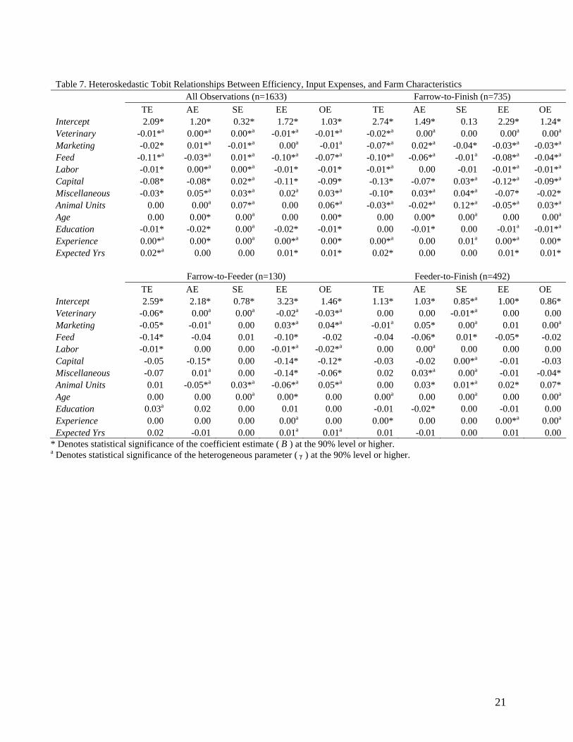
Table 7. Heteroskedastic Tobit Relationships Between Efficiency, Input Expenses, and Farm Characteristics All Observations (n=1633) Farrow-to-Finish (n=735) TE AE SE EE OE TE AE SE EE OE Intercept 2.09* 1.20* 0.32* 1.72* 1.03* 2.74* 1.49* 0.13 2.29* 1.24* Veterinary -0.01*a 0.00*a 0.00*a -0.01*a -0.01*a -0.02*a 0.00a 0.00 0.00a 0.00a

Marketing -0.02* 0.01*a -0.01*a 0.00a -0.01a -0.07*a 0.02*a -0.04* -0.03*a -0.03*a

Feed -0.11*a -0.03*a 0.01*a -0.10*a -0.07*a -0.10*a -0.06*a -0.01a -0.08*a -0.04*a

Labor -0.01* 0.00*a 0.00*a -0.01* -0.01* -0.01*a 0.00 -0.01 -0.01*a -0.01*a

Capital -0.08* -0.08* 0.02*a -0.11* -0.09* -0.13* -0.07* 0.03*a -0.12*a -0.09*a

Miscellaneous -0.03* 0.05*a 0.03*a 0.02a 0.03*a -0.10* 0.03*a 0.04*a -0.07* -0.02* Animal Units 0.00 0.00a 0.07*a 0.00 0.06*a -0.03*a -0.02*a 0.12*a -0.05*a 0.03*a

Age 0.00 0.00* 0.00a 0.00 0.00* 0.00 0.00* 0.00a 0.00 0.00a

Education -0.01* -0.02* 0.00a -0.02* -0.01* 0.00 -0.01* 0.00 -0.01a -0.01*a

Experience 0.00*a 0.00* 0.00a 0.00*a 0.00* 0.00*a 0.00 0.01a 0.00*a 0.00* Expected Yrs 0.02*a 0.00 0.00 0.01* 0.01* 0.02* 0.00 0.00 0.01* 0.01* Farrow-to-Feeder (n=130) Feeder-to-Finish (n=492) TE AE SE EE OE TE AE SE EE OE Intercept 2.59* 2.18* 0.78* 3.23* 1.46* 1.13* 1.03* 0.85*a 1.00* 0.86* Veterinary -0.06* 0.00a 0.00a -0.02a -0.03*a 0.00 0.00 -0.01*a 0.00 0.00 Marketing -0.05* -0.01a 0.00 0.03*a 0.04*a -0.01a 0.05* 0.00a 0.01 0.00a

Feed -0.14* -0.04 0.01 -0.10* -0.02 -0.04 -0.06* 0.01* -0.05* -0.02 Labor -0.01* 0.00 0.00 -0.01*a -0.02*a 0.00 0.00a 0.00 0.00 0.00 Capital -0.05 -0.15* 0.00 -0.14* -0.12* -0.03 -0.02 0.00*a -0.01 -0.03 Miscellaneous -0.07 0.01a 0.00 -0.14* -0.06* 0.02 0.03*a 0.00a -0.01 -0.04* Animal Units 0.01 -0.05*a 0.03*a -0.06*a 0.05*a 0.00 0.03* 0.01*a 0.02* 0.07* Age 0.00 0.00 0.00a 0.00* 0.00 0.00a 0.00 0.00a 0.00 0.00a

Education 0.03a 0.02 0.00 0.01 0.00 -0.01 -0.02* 0.00 -0.01 0.00 Experience 0.00 0.00 0.00 0.00a 0.00 0.00* 0.00 0.00 0.00*a 0.00a

Expected Yrs 0.02 -0.01 0.00 0.01a 0.01a 0.01 -0.01 0.00 0.01 0.00 * Denotes statistical significance of the coefficient estimate ( ) at the 90% level or higher. Ba Denotes statistical significance of the heterogeneous parameter ( ) at the 90% level or higher.γ

21

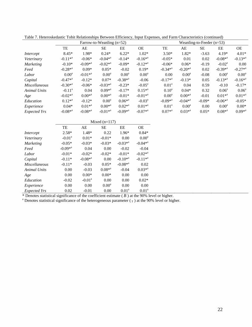
Table 7. Heteroskedastic Tobit Relationships Between Efficiency, Input Expenses, and Farm Characteristics (continued) Farrow-to-Weanling (n=52) Weanling-to-Feeder (n=53) TE AE SE EE OE TE AE SE EE OE Intercept 8.45* 1.98* 0.24* 6.22* 1.02* 3.50* 1.82* -3.63 4.19* 4.01* Veterinary -0.11*a -0.06* -0.04*a -0.14* -0.16*a -0.05* 0.01 0.02 -0.08*a -0.13*a

Marketing -0.10* -0.09*a -0.02*a -0.09* -0.12*a -0.06* 0.06* -0.19 -0.02a 0.00 Feed -0.28*a 0.09* 0.05* -0.02 0.19* -0.34*a -0.20*a 0.02 -0.39*a -0.27*a

Labor 0.00a -0.01*a 0.00a 0.00a 0.00a 0.00 0.00a -0.08 0.00a 0.00a

Capital -0.47*a -0.12* 0.07* -0.38*a -0.06 -0.17*a -0.13* 0.05 -0.13*a -0.16*a

Miscellaneous -0.30*a -0.06* -0.03*a -0.23* -0.05a 0.01a 0.04 0.59 -0.10 -0.17* Animal Units -0.11a 0.04 0.09*a -0.17* 0.15*a 0.10a 0.04* 0.32 0.06a 0.06a

Age -0.02*a 0.00*a 0.00*a -0.01* -0.01*a 0.00a 0.00*a -0.01 0.01*a 0.01*a

Education 0.12*a -0.12* 0.00a 0.06*a -0.03a -0.09*a -0.04*a -0.09* -0.06*a -0.05* Experience 0.04* 0.01*a 0.00*a 0.02*a 0.01*a 0.01a 0.00a 0.00 0.00a 0.00* Expected Yrs -0.08*a -0.08*a -0.01*a -0.09*a -0.07*a 0.07*a 0.03*a 0.05* 0.08*a 0.09*a

Mixed (n=117) TE AE SE EE OE Intercept 2.58* 1.48* 0.22 1.96* 0.84* Veterinary -0.01a 0.01* -0.01* 0.00 0.00a Marketing -0.05* -0.03* -0.03* -0.03*a -0.04*a Feed -0.09*a 0.04 0.00 -0.02 -0.04 Labor -0.01* -0.02* -0.02* -0.01* -0.02*a Capital -0.11* -0.08*a 0.00 -0.10*a -0.11*a Miscellaneous -0.11* -0.03 0.05* -0.08*a 0.02 Animal Units 0.00 -0.03 0.08*a -0.04 0.03*a Age 0.00 0.00* 0.00* 0.00 0.00 Education -0.02 -0.01a 0.00 0.00 0.02* Experience 0.00 0.00 0.00a 0.00 0.00 Expected Yrs 0.02 -0.01 0.00 0.01a 0.01a

* Denotes statistical significance of the coefficient estimate ( ) at the 90% level or higher. Ba Denotes statistical significance of the heterogeneous parameter ( ) at the 90% level or higher. γ

22

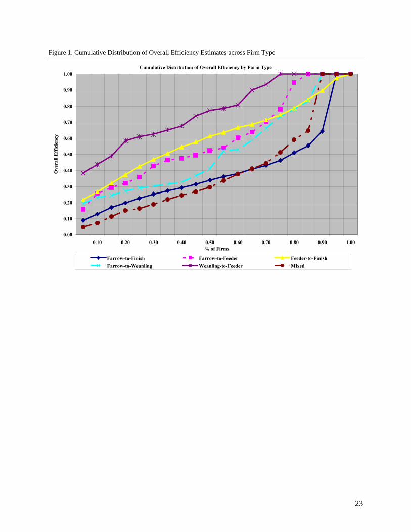
Figure 1. Cumulative Distribution of Overall Efficiency Estimates across Firm Type

Cumulative Distribution of Overall Efficiency by Farm Type

0.00

0.10

0.20

0.30

0.40

0.50

0.60

0.70

0.80

0.90

1.00

0.10 0.20 0.30 0.40 0.50 0.60 0.70 0.80 0.90 1.00% of Firms

Ove

rall

Eff

icie

ncy

Farrow-to-Finish Farrow-to-Feeder Feeder-to-FinishFarrow-to-Weanling Weanling-to-Feeder Mixed

23