Heterogeneous Costs of Business Cycles

with Incomplete Markets∗

Toshihiko Mukoyama

Department of Economics

Concordia University

and

CIREQ

Aysegul Sahin†

Department of Economics

Purdue University

February 12, 2004

Abstract

This paper reconsiders the cost of business cycles under market incompleteness. Pri-marily, we focus on the heterogeneity in the cost among different groups. In addition tothe heterogeneity in asset holdings, this paper considers heterogeneity in earnings andunemployment risk. In particular, we focus on skill heterogeneity. Unskilled workers aresubject to a much larger risk of unemployment during recessions than are skilled workers.This serves as an additional source of heterogeneity in the cost of business cycles. Thiseffect is reinforced by the fact that unskilled workers earn less, so that they have lessresources for precautionary saving.

Keywords: Cost of Business Cycles; Incomplete Markets; Skill and Unemployment

JEL Classifications: E24, E32; E61

∗The discussions with Per Krusell and Tony Smith were very helpful. We thank Sun-Bin Kim for his help

in Fortran programming. We also thank Mark Bils, Emanuela Cardia, Rui Castro, Igor Livshits, and seminar

participants at Indiana University, University of Illinois at Urbana-Champaign, the Montreal Macro Reading

Group, the Rochester Wegmans Conference, the CEA Annual Meetings 2003, and the Society for Economic

Dynamics Meetings 2003 for comments and suggestions. We thank Vera Brencic and Roxanne Stanoprud for

excellent research assistance. All errors are our own. Mukoyama thanks FQRSC for financial support.†Corresponding author. Address: Purdue University, Krannert School of Management, 403 W. State

St. West Lafayette, IN 47907-2056. Tel.: +1-765-494-4419; fax: +1-765-494-9658. E-mail address:

asahin@mgmt.purdue.edu.

1

1 Introduction

In everyday discussions of economic policy, it is usually assumed that business cycles are evil

and that it is desirable to eliminate them. Many would agree that stabilization is desirable

if it comes without cost. However, stabilization policies are often very costly, and it is not

obvious whether we should avoid business cycles when the cost of doing so is great. What,

in fact, is the cost of having business cycles? How much resource cost can be justified to

eliminate business cycles? In an influential study, Lucas (1987) considered these questions.

His result was astounding – the cost of having business cycles is almost zero.

Lucas’s method is simple. Postulate a standard utility function for a representative

agent. Feed a consumption series that resembles the actual aggregate consumption time

series into the utility function, and calculate the utility that the representative agent obtains

from the consumption stream. Compare this with the utility from a smoothed version of

the consumption series (the mean of the original consumption series). How much is the

representative agent willing to pay for moving from the fluctuating consumption path to

the smooth consumption path? This amount is the measure of the cost of business cycles.

Specifically, Lucas calculates λ which satisfies

E0

[ ∞∑

t=0

βtU((1 + λ)cot )

]= E0

[ ∞∑

t=0

βtU(cst )

], (1)

where cot∞t=0 is the consumption stream in the original economy (with business cycles), and

cst∞t=0 is the consumption stream in the “smoothed” economy (without business cycles). He

finds λ = 0.008% with logarithmic utility.

Some researchers interpreted Lucas’s result to indicate that neither the policy nor the re-

search aimed at coping with business cycles is thus relevant. Many other researchers felt that

the number Lucas obtained was too small, and challenged Lucas’s assumptions. There are

three strands of literature that re-examine Lucas’s calculation. The first challenges Lucas’s

assumptions on preferences and the nature of the stochastic process of consumption (e.g. Ob-

2

stfeld [1994]). If, for example, the consumer’s risk aversion is larger, or the stochastic process

is not stationary, then the cost of business cycles will be larger. The second asserts that the

elimination of business cycles affects the output trend of the economy (e.g. Barlevy [2002]).

The third argues that Lucas’s use of a representative agent and an aggregate consumption

series is not realistic, and considers different model environments. This paper extends this

third line of argument.

Lucas’s use of a representative agent and an aggregate consumption series are justified in

an environment where complete Arrow-Debreu markets exist. Under complete asset markets

and a common constant relative risk aversion utility function, the aggregation theorem holds

and the consumption series of each individual will parallel the aggregate consumption series.

In reality however, it is unlikely that the asset markets are complete.

Recent macroeconomic studies focus increasingly more on an environment where asset

markets are not complete. The incompleteness of asset markets can potentially have a large

impact on the calculation of the cost of business cycles, since the opportunity for insuring risk

is limited in such an environment. Imrohoroglu (1989) was the first to attempt to measure the

welfare cost of business cycles under market incompleteness. She considers an environment

where individuals face idiosyncratic unemployment risk, and they cannot insure each other

because asset markets are not complete. By comparing environments where aggregate shocks

are present and then removed, she obtained a larger cost of business cycles than Lucas did.

When the coefficient of relative risk aversion is 1.5, the cost is equivalent to 0.3% of average

consumption.

Atkeson and Phelan (1994) re-examined the welfare effect of eliminating business cycles

under market incompleteness. When considering the economy without business cycles, in-

stead of removing the aggregate shocks (as Imrohoroglu did), they removed the correlation

of aggregate shocks across individuals. Thus, although aggregate fluctuations are removed,

individuals essentially face the same shocks. The resulting cost of business cycles is much

3

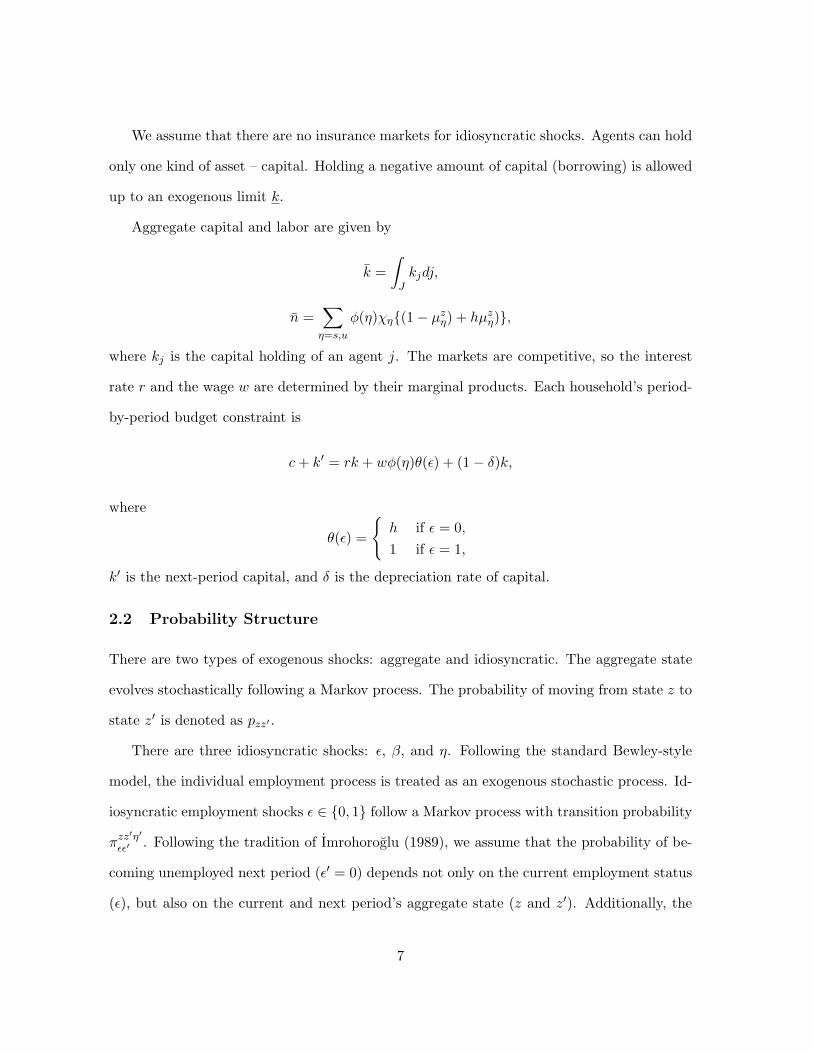
1970 1975 1980 1985 1990 1995 20000

2

4

6

8

10

12

14

unem

ploy

men

t rat

e (%

)

year

unskilled

skilled

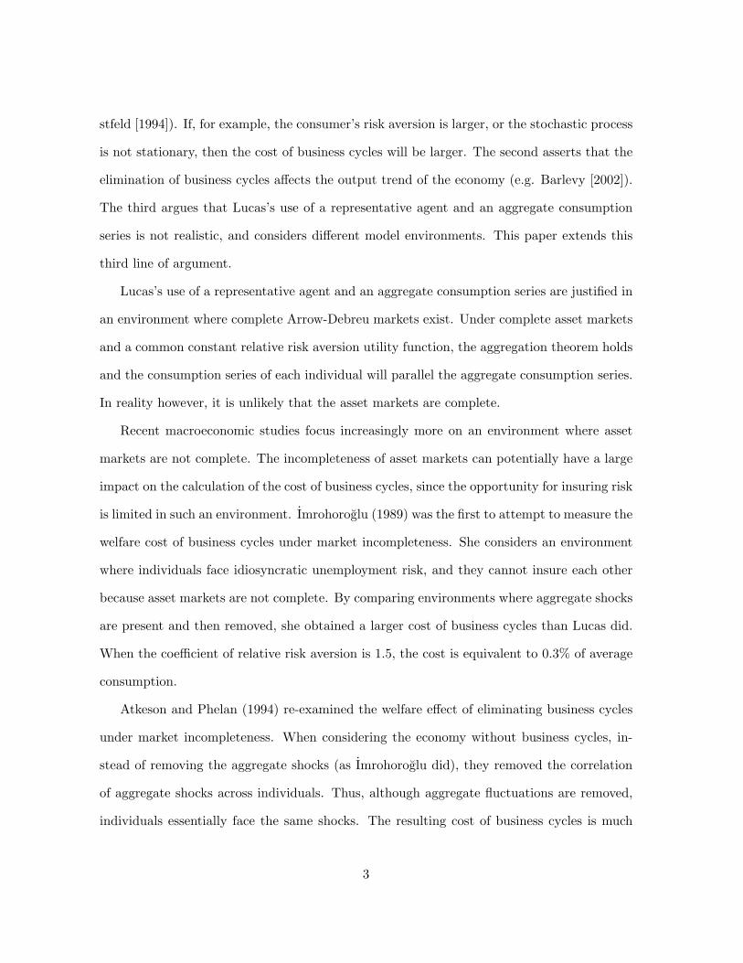
Figure 1: Unemployment Rates by Skill.Data Source: Current Population Survey

smaller than that in Imrohoroglu (1989): λ = 0.02% on average, when the coefficient of risk

aversion is 1.35.

Krusell and Smith (1999, 2002) analyzed a dynamic general equilibrium model with en-

dogenous prices which matches the U.S. wealth distribution. They proposed a method called

the “integration principle” when removing business cycles. They argued that the part of the

idiosyncratic shocks which is correlated with the aggregate shocks should be removed when

business cycles are eliminated. Their result (Krusell and Smith [2002]) is that λ = 0.09% on

average with logarithmic utility.

Perhaps more importantly, Krusell and Smith (1999, 2002) pointed out that the cost of

business cycles may differ among different groups of people. For example, agents with larger

asset holdings would have a greater opportunity to self-insure against unemployment risk. It

can be expected that very poor agents would have a larger cost of business cycles. Krusell and

Smith (1999, 2002) reported that there is considerable heterogeneity in the cost of business

cycles among agents with different wealth.

4

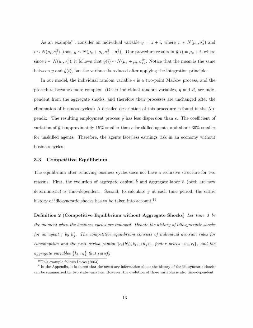
We extend Krusell and Smith’s analysis to the case where there is an additional source of

heterogeneity. Our analysis is motivated by the microeconomic studies of the unemployment

process. Figure 1 is drawn from the annual data in the Current Population Survey (1970–

2001). It illustrates the unemployment processes for unskilled workers (high school diploma or

lower) and for skilled workers (some college or above). The two processes differ dramatically.

Unskilled workers are not only subject to higher level of unemployment, but also face a

more volatile unemployment process. This implies that unskilled workers are hurt more by

recessions.1 Moreover, unskilled workers earn less income, which limits their ability to self-

insure. We examine how this heterogeneity in unemployment risk and income translates into

heterogeneity in the cost of business cycles.

This paper is organized as follows. The next section describes our baseline model. In

Section 3, we analyze the welfare effects of removing business cycles. Section 4 concludes.

2 Model

2.1 Setup

Our model is a standard Bewley-Aiyagari type dynamic general equilibrium model with

incomplete markets (Aiyagari [1994]). In particular, we build upon the model with aggregate

shocks developed by Krusell and Smith (1998).

There is a continuum of agents (with measure 1) in the economy. They maximize their

discounted utility

U = E0

∞∑

t=0

(t∏

j=0

βj) log ct

,

where ct is the consumption in period t and β0 = 1. We allow the discount factor βt to differ

across agents and to vary over time.1Mincer (1991) documented that unskilled workers are subject to a substantially larger risk of becoming

unemployed in recessions than are skilled workers. Topel (1993) shows that the unemployment rate of low-wage

men is not only higher, but also much more volatile.

5

There are two types of agents: skilled (η = s) and unskilled (η = u). Each agent’s skill

status η may change over time (by a stochastic process that is uncorrelated across agents),

but the number of skilled (χs) and unskilled (χu) workers is constant by the law of large

numbers. A skilled worker can supply more labor than an unskilled worker. We express

this dependence by the function φ(η), where φ(s) > φ(u). The value φ(s)/φ(u) can be

interpreted as the skill premium. We assume that φ(η) is constant over time. Therefore, the

skill premium is acyclical.2

An agent is either employed (ε = 1) or unemployed (ε = 0). The employment status is

determined by an exogenous random process. When employed, the agent supplies φ(η) units

of labor to the market. When unemployed, she engages in household production. Household

production utilizes the same technology as the market technology3, but the agent can supply

only a fraction h < 1 of her market labor supply (she is less efficient at home than in the

market).4 The probability of becoming unemployed differs between skilled and unskilled

agents. The unemployment probability also depends on the aggregate state of the economy.

The market technology is represented by the aggregate production function

Y = zkαn1−α,

where k is the aggregate capital and n is the aggregate labor (including the labor supplied

for household production). The economy is subject to aggregate shocks. The aggregate state

is either good or bad. In a good state, z = g and the unemployment rate for skill level η is

µgη. In a bad state, z = b and the unemployment rate for skill level η is µb

η. We assume that

g > b and µgη < µb

η for η = s, u; i.e., productivity is higher and the unemployment rate is

lower in booms than in recessions.2This assumption is motivated by the empirical studies by Raisian (1983) and Keane and Prasad (1993).3It is implicitly assumed that a worker can rent capital for household production without limit. This

assumption is not inconsistent with the household borrowing constraint, introduced below, if the household

production capital can be collateralized perfectly.4This assumption is made so that an agent can earn some labor income even when she is unemployed.

Alternatively, we can introduce an unemployment insurance system a la Hansen and Imrohoroglu (1992). In

this case, a government and its budget constraint would need to be incorporated into our setup.

6

We assume that there are no insurance markets for idiosyncratic shocks. Agents can hold

only one kind of asset – capital. Holding a negative amount of capital (borrowing) is allowed

up to an exogenous limit k.

Aggregate capital and labor are given by

k =∫

Jkjdj,

n =∑

η=s,u

φ(η)χη(1− µzη) + hµz

η),

where kj is the capital holding of an agent j. The markets are competitive, so the interest

rate r and the wage w are determined by their marginal products. Each household’s period-

by-period budget constraint is

c + k′ = rk + wφ(η)θ(ε) + (1− δ)k,

where

θ(ε) =

h if ε = 0,

1 if ε = 1,

k′ is the next-period capital, and δ is the depreciation rate of capital.

2.2 Probability Structure

There are two types of exogenous shocks: aggregate and idiosyncratic. The aggregate state

evolves stochastically following a Markov process. The probability of moving from state z to

state z′ is denoted as pzz′ .

There are three idiosyncratic shocks: ε, β, and η. Following the standard Bewley-style

model, the individual employment process is treated as an exogenous stochastic process. Id-

iosyncratic employment shocks ε ∈ 0, 1 follow a Markov process with transition probability

πzz′η′εε′ . Following the tradition of Imrohoroglu (1989), we assume that the probability of be-

coming unemployed next period (ε′ = 0) depends not only on the current employment status

(ε), but also on the current and next period’s aggregate state (z and z′). Additionally, the

7

probability of becoming unemployed depends on the skill level in the next period (η′), to

reflect the heterogeneity exhibited in Figure 1.

The discount factor β is assumed to be stochastic. At each point in time some agents

are more patient than others. We interpret each agent as an altruistic dynasty. Each agent’s

patience level may differ across generations. This formulation serves as a device to produce

a realistic wealth distribution.5 We assume that β’s process is independent of the other

aggregate and idiosyncratic state variables. The Markov transition probability is denoted as

ωββ′ .

We assume that the individual skill level η ∈ u, s follows an exogenous stochastic

process. This transition probability is denoted as qηη′ . Again, we can interpret each agent

as an altruistic dynasty. Within each dynasty, the skill level may differ across generations.

The probability qηη′ reflects the intergenerational mobility of skill levels.6 The skill transition

process is assumed to be independent of the other state variables.7

2.3 Recursive Competitive Equilibrium

Let Γ denote the measure of agents over (k, ε, η, β). The state variables relevant to each indi-

vidual are the aggregate state variables (z,Γ) and the idiosyncratic state variables (k, ε, η, β).

Let T denote the equilibrium transition function for Γ:

Γ′ = T(Γ, z, z′).

Definition 1 (Recursive Competitive Equilibrium) The recursive competitive equilib-

rium consists of the value function v(k, ε, η, β; z, Γ), a set of decision rules for consumption

and asset holdings c(k, ε, η, β; z, Γ), k′(k, ε, η, β; z,Γ), aggregate capital and labor k(z,Γ), n(z,Γ),5This method was first developed by Krusell and Smith (1998).6In our formulation, the timing of the switch in β and η may not coincide. Synchronizing these processes

is possible, but it complicates the analysis considerably and would not substantially alter our main results.7Belzil and Hansen (2003) estimate a structural model of educational choice and argue that the difference

in discount rates has little effect on educational choice.

8

factor prices w(z, Γ), r(z, Γ), and a law of motion for the distribution, Γ′ = T(Γ, z, z′),

which satisfy

1. Given the aggregate states, z,Γ, prices w(z,Γ), r(z,Γ), and the law of motion for

the distribution, Γ′ = T(Γ, z, z′); the value function v(k, ε, η, β; z,Γ) and the individual

decision rules c(k, ε, η, β; z, Γ), k′(k, ε, η, β; z,Γ) solve the following dynamic program-

ming problem:

v(k, ε, η, β; z, Γ) = maxc,k′

log c + βE[v(k′, ε′, η′, β′; z′, Γ′)|ε, η, β, z,Γ]

subject to

c + k′ = r(z, Γ)k + w(z, Γ)φ(η)θ(ε) + (1− δ)k,

k′ ≥ k,

and

Γ′ = T(Γ, z, z′).

2. Firms optimize:

w(z, Γ) = (1− α)zkαn−α,

r(z, Γ) = αzkα−1n1−α.

3. Markets clear:

k =∫

kdΓ,

n =∫

φ(η)θ(ε)dΓ.

4. Consistency:

Γ′(K, E,X, B) =∫

K,E,X,B

[∫

K,E,X ,BIk′=k′(k,ε,η,β;z,Γ)π

zz′η′εε′ qηη′ωββ′dΓ

]dk′dε′dη′dβ′

for all K ⊂ K, E ⊂ E, X ⊂ X , and B ⊂ B. K, E, X , and B are the sets of all possible

realizations of k, ε, η, and β, respectively. The indicator function I· takes the value

9

1 if the statement is true, and 0 if it is false. The transition probabilities πzz′η′εε′ , qηη′,

and ωββ′ are defined in the Appendix.

2.4 Calibration

We follow a standard calibration for the most part. One period is considered to be six weeks.

We choose δ = 0.0125 and the average value of β as 0.995. The capital share α = 0.36.

Aggregate shocks take the values z ∈ 0.99, 1.01, and pzz′ is chosen so that the average

duration of each aggregate state is 2 years. The household production parameter h is assumed

to be 0.1. These numbers closely follow the calibration of Krusell and Smith (1999, 2002). The

borrowing constraint k is set at −13, which is tighter than the “always payback constraint”.

This number is chosen so that the fraction of the people with negative wealth mimics the

actual data.

The idiosyncratic probabilities πzz′η′εε′ and qηη′ are chosen so that the processes of unem-

ployment and intergenerational mobility of education mimic the data. The process of β is

chosen so that the resulting wealth distribution parallels the real-life wealth distribution.

The skill premium, φ(s)/φ(u), is set to 1.50. Details on how we calibrated the stochastic

processes and the skill premium are found in the Appendix.

2.5 Model Solution

Generally, it is computationally burdensome to solve this type of model. The state variables

in the individual optimization include the economy-wide wealth distribution, which is an

infinite-dimensional object. In our model, the wealth distribution is in the state variables,

since this information is necessary for predicting the next-period prices (for each aggregate

state). To predict these prices, the agents have to predict the next period’s aggregate capi-

tal, which requires knowledge of the current period’s wealth distribution. Krusell and Smith

(1998) developed a computational method to overcome this obstacle. They found that knowl-

edge of only a few moments of the wealth distribution is often sufficient for predicting the

10

next period’s aggregate capital. In fact, they demonstrated that a linear prediction rule

based only on the first moment k provides very accurate prediction. They call their method

“approximate aggregation”.

This method works very well in our setting. In our model, we postulate a prediction rule

ln k′ = α0 + α1 ln k + α2 ln z.

The coefficients α0 = 0.1152, α1 = 0.9768, and α2 = 0.0916 provide a very accurate predic-

tion. The R2 of this prediction rule is 0.99998.

The aggregate capital fluctuates between the values k = 140.2 and k = 149.7. For the

most part, k is contained in between 142 and 148. On average, skilled agents hold k = 184.1

and unskilled agents hold k = 104.7. Since the earning ratio is 1 : 1.5, the difference in

asset holdings is more pronounced than the earnings difference.8 This large difference in

asset holding is important, since wealth holdings are the only means of self-insurance for

unemployment in our incomplete-market setting.

The wealth distribution is matched to the data. In the data9 the Gini coefficient of the

wealth distribution is 0.80, while in the model, it is 0.79. In the right tail of the distribution,

the top 10% of wealth-rich people hold about 69% of the real economy’s total wealth, while

68% of wealth is held by the top 10% in the model. In the data, the top 20% (fifth wealth

quintile) hold 82% of the total wealth, while the corresponding number is 84% in the model.

In the left tail of the distribution, in the model approximately 8% of the agents hold negative

wealth. In the data, 7.4% of the population report negative wealth and 2.5% report zero

wealth. In the model, less than 2% hold negative wealth within the group of skilled agents,

while nearly 15% of unskilled agents fall into this category. The model produces more wealth8This property can also be seen in data. The average wealth-earnings ratio of a college graduate is higher

than that of a high school graduate. See Burdıa Rodrıguez, Dıaz-Gimenez, Quadrini, and Rıos-Rull (2002).9All the data in this paragraph are drawn from Burdıa Rodrıguez, Dıaz-Gimenez, Quadrini, and Rıos-Rull

(2002). Wolff (1995) employs a slightly different definition of wealth (most notable difference is that he does

not include vehicles and pension plans). In Wolff (1995), top 20% hold 85% of the total wealth and the Gini

coefficient is 0.84.

11

inequality within unskilled agents than within skilled agents: Gini coefficients are 0.86 and

0.71, respectively.

3 Removing Business Cycles

The main question to be answered is: what will happen to people’s welfare when business

cycles are eliminated? To answer this, we follow Lucas’s tradition in not describing specific

policies to eliminate cycles. We directly eliminate shocks that are driving the aggregate

fluctuations. The elimination is permanent, and this event is unanticipated by the agents.

3.1 Aggregate Shocks

Since the aggregate shocks are the driving force of the business cycles, a natural way to

eliminate cycles is to replace the aggregate stochastic process by a deterministic process. In

the spirit of Lucas, we replace the aggregate stochastic process by its conditional mean. The

aggregate state z starts at z = 1.01 or z = 0.99 depending on the timing of the removal, and

z converges monotonically to the value 1, which is the unconditional mean of z.

3.2 Idiosyncratic Shocks

We assume that when the business cycles are eliminated, the part of the idiosyncratic risk

which is correlated with the aggregate shocks is also eliminated. Krusell and Smith (1999,

2002), who first proposed this procedure coined it the “integration principle”. Formally,

when an idiosyncratic random variable y can be written as a function g(i, z) of the aggregate

variable z and a random variable i which is independent from z, then the new idiosyncratic

variable after the elimination of the cycles is given by

y(i) =∫

g(i, z)fz(z)dz, (2)

with density fi(i) for each i. Here, fz(z) and fi(i) are the marginal density functions for z

and i, respectively.

12

As an example10, consider an individual variable y = z + i, where z ∼ N(µz, σ2z) and

i ∼ N(µi, σ2i ) [thus, y ∼ N(µz + µi, σ

2z + σ2

i )]. Our procedure results in y(i) = µz + i, where

since i ∼ N(µi, σ2i ), it follows that y(i) ∼ N(µz + µi, σ

2i ). Notice that the mean is the same

between y and y(i), but the variance is reduced after applying the integration principle.

In our model, the individual random variable ε is a two-point Markov process, and the

procedure becomes more complex. (Other individual random variables, η and β, are inde-

pendent from the aggregate shocks, and therefore their processes are unchanged after the

elimination of business cycles.) A detailed description of this procedure is found in the Ap-

pendix. The resulting employment process y has less dispersion than ε. The coefficient of

variation of y is approximately 15% smaller than ε for skilled agents, and about 30% smaller

for unskilled agents. Therefore, the agents face less earnings risk in an economy without

business cycles.

3.3 Competitive Equilibrium

The equilibrium after removing business cycles does not have a recursive structure for two

reasons. First, the evolution of aggregate capital k and aggregate labor n (both are now

deterministic) is time-dependent. Second, to calculate y at each time period, the entire

history of idiosyncratic shocks has to be taken into account.11

Definition 2 (Competitive Equilibrium without Aggregate Shocks) Let time 0 be

the moment when the business cycles are removed. Denote the history of idiosyncratic shocks

for an agent j by htj. The competitive equilibrium consists of individual decision rules for

consumption and the next period capital ct(htj), kt+1(ht

j), factor prices wt, rt, and the

aggregate variables kt, nt that satisfy10This example follows Lucas (2003).11In the Appendix, it is shown that the necessary information about the history of the idiosyncratic shocks

can be summarized by two state variables. However, the evolution of those variables is also time-dependent.

13

1. Given wt, rt, consumers optimize:

E0

∞∑

t=0

(t∏

j=0

βj) log ct,

with β0 = 1, subject to

ct + kt+1 = rtkt + wtφ(ηt)yt + (1− δ)kt,

kt+1 ≥ k.

2. Firms optimize:

wt = (1− α)kαt n−α

t ,

rt = αkα−1t n1−α

t .

3. Markets clear:

kt =∫

Jkt,jdj,

where kt,j is the asset holding of an agent j at time t,

n =∫

φ(ηt)ytdΓt,

where Γt is the measure over ηt and yt.

We employ three approximations to reduce the computational burden. First, since n

converges to a constant value fairly quickly, we treat n as a constant after a sufficient number

of periods. Second, we reduce the evolution of k to a single law of motion after a sufficient

number of periods. Third, we approximate the stochastic process of y by a five-point Markov

process. These approximations serve to reduce the computational time dramatically, while

providing a fairly accurate approximation of the original economy.

14

3.4 Results

Our experiment is to eliminate business cycles at a specific point from the fluctuating econ-

omy.12 The timing of this “elimination” (call it time 0) is selected according to a specific

level of capital stock and aggregate shocks. We select four timings:

1. k = 146 and z = g,

2. k = 146 and z = b,

3. k = 144 and z = g,

4. k = 144 and z = b.

After time 0, the economy experiences the transition to a non-fluctuating steady state. We

compare the welfare of each agent at time 0, taking this transition into account.

3.4.1 Case 1: k = 146 and z = g

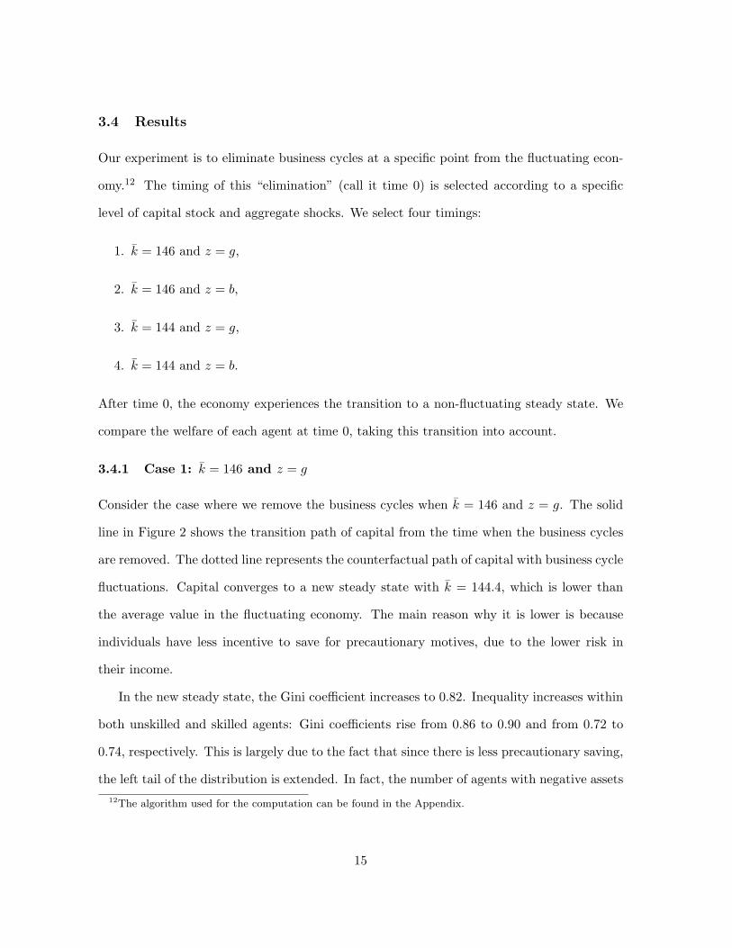
Consider the case where we remove the business cycles when k = 146 and z = g. The solid

line in Figure 2 shows the transition path of capital from the time when the business cycles

are removed. The dotted line represents the counterfactual path of capital with business cycle

fluctuations. Capital converges to a new steady state with k = 144.4, which is lower than

the average value in the fluctuating economy. The main reason why it is lower is because

individuals have less incentive to save for precautionary motives, due to the lower risk in

their income.

In the new steady state, the Gini coefficient increases to 0.82. Inequality increases within

both unskilled and skilled agents: Gini coefficients rise from 0.86 to 0.90 and from 0.72 to

0.74, respectively. This is largely due to the fact that since there is less precautionary saving,

the left tail of the distribution is extended. In fact, the number of agents with negative assets12The algorithm used for the computation can be found in the Appendix.

15

0 50 100 150 200 250 300141

142

143

144

145

146

147

148

149

time

aggr

egat

e ca

pita

l

Figure 2: Path of Aggregate Capital after Removing Business Cycles

increases to 15.7% in total (27.4% for unskilled and 4.1% for skilled), which is almost twice

compared to the fluctuating economy.

Our main goal is to compare the welfare between the two economies. We follow Lucas’s

method (1), and calculate the value of λ for each agent. Details of the calculation is delegated

to the Appendix. The average value of λ is 0.028%, which is more than three times larger

than Lucas’s, and comparable to the numbers found in previous studies by Atkeson and

Phelan (1994) and Krusell and Smith (2002). There is a large heterogeneity between skill

levels: unskilled agents gain 0.069% from the elimination of business cycles, while skilled gain

only 0.008%. As a result of stabilization, 93.1% of unskilled workers have increased utility

while the fraction of skilled workers with a positive gain is much smaller at 42.9%. In fact, the

majority of skilled workers experience lower utility by stabilization. Two effects produce the

difference in costs of business cycles between skilled and unskilled workers. First, a majority

of the skilled agents already accumulated enough wealth to insure themselves against the

idiosyncratic risk. Unskilled workers tend to gain more since their level of wealth is lower on

average. Second, at an individual level, the unskilled agents were facing larger unemployment

16

asset level (in total wealth distribution)constrained bottom 1% 50% 99% 99.9%

η = u, ε = 0 0.177% 0.093% -0.022% -0.002% 0.119%

η = u, ε = 1 0.145% 0.118% 0.047% 0.017% 0.129%

η = s, ε = 0 0.068% 0.008% -0.071% -0.005% 0.090%

η = s, ε = 1 0.043% 0.030% -0.005% 0.021% 0.108%

Table 1: The values of λ for β = 0.995

risk under business cycle fluctuations. There is also the general equilibrium effect (discussed

below), whose direction is ambiguous.

The costs at an individual level are shown in Table 1. We focus on the agents with

β = 0.995.13 We observe even larger heterogeneity at an individual level. For example, a

wealth-constrained agent with η = u (unskilled) and ε = 0 (unemployed) realizes more than

six times larger cost than on average. (Those are the agents whose cost is the highest.) This

figure, 0.177%, is more than twenty-two times larger than the number obtained by Lucas.14

Tables in the Appendix show that if we eliminate the cycles when the aggregate state is bad,

the largest cost is more than 0.75%, which is more than ninety times larger than Lucas’s

number.

When considering the welfare effect on individuals, two factors have to be taken into

account.

1. Direct effect of the risk reduction.

2. General equilibrium effect.

The first is straightforward. When business cycles are eliminated, the aggregate shocks are

completely smoothed out (the interest rate and the wage become deterministic variables),13Heterogeneity of the costs across different β is discussed in detail by Krusell and Smith (2002).14It is somewhat smaller than the number that Krusell and Smith (2002) obtained. There are two factors

that reduce our numbers compared to theirs. First, in our calibration, the average duration of unemployment

is substantially shorter than Krusell and Smith’s. Second, our borrowing constraint is tighter, therefore the

“constrained agents” here are not as wealth-poor as Krusell and Smith’s.

17

and the idiosyncratic employment risk is also reduced. This benefits all agents, especially

the agents who cannot self-insure by their own savings. The second effect calls for a more

careful analysis. Since the steady-state capital is lower after eliminating the business cycles

(because of less precautionary saving), on average, the interest rate rises and the wage falls.

This benefits an agent for whom capital income is more important than wage income.

Keeping the employment status and skill status constant (within each rows of Table 1), the

gains from eliminating business cycles exhibit a “U-shape” pattern.15 Borrowing-constrained

agents have a larger gain, reflecting the fact that they cannot self-insure their risk by their

own assets. The direct effect of the reduction in idiosyncratic risk is very large for these

agents. The “middle class” tends to have small or negative gains. For these agents, the

benefit from the reduction in the idiosyncratic risk is small, since they have enough assets to

insure themselves. In this case, the general equilibrium effect dominates. The middle-class

agents whose income is largely coming from wage may experience lower welfare due to the

wage loss. Very rich agents realize welfare gains since their income is largely coming from

capital income.

Keeping the wealth level constant (within each columns of Table 1), we cannot always

determine whether employed agents gain more than unemployed agents, or if skilled agents

gain more than unskilled agents, due to the presence of the general equilibrium effect.

For the borrowing-constrained agents, it is usually possible to make a definite comparison,

since the direct effect of the risk reduction dominates the other effects. For the constrained

agents, the unemployed agents gain more than the employed agents, and the unskilled agents

gain more than the skilled agents. This is due to the simple fact that the unemployed and the

unskilled agents have smaller chances of getting out of the borrowing-constrained situation,

compared to the the employed and the skilled agents, and therefore the direct benefit from

the risk reduction is larger for them.15This pattern is also observed in Krusell and Smith (2002).

18

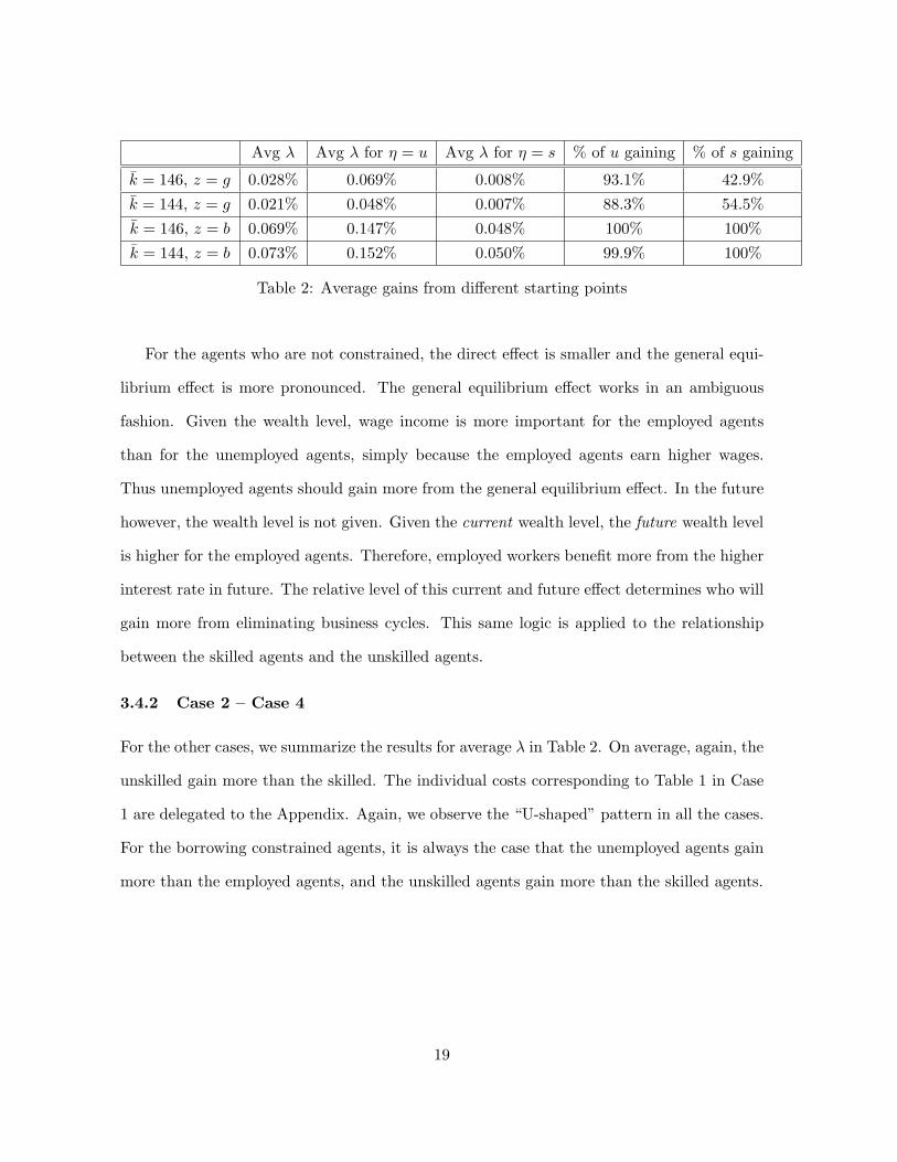
Avg λ Avg λ for η = u Avg λ for η = s % of u gaining % of s gaining

k = 146, z = g 0.028% 0.069% 0.008% 93.1% 42.9%

k = 144, z = g 0.021% 0.048% 0.007% 88.3% 54.5%

k = 146, z = b 0.069% 0.147% 0.048% 100% 100%

k = 144, z = b 0.073% 0.152% 0.050% 99.9% 100%

Table 2: Average gains from different starting points

For the agents who are not constrained, the direct effect is smaller and the general equi-

librium effect is more pronounced. The general equilibrium effect works in an ambiguous

fashion. Given the wealth level, wage income is more important for the employed agents

than for the unemployed agents, simply because the employed agents earn higher wages.

Thus unemployed agents should gain more from the general equilibrium effect. In the future

however, the wealth level is not given. Given the current wealth level, the future wealth level

is higher for the employed agents. Therefore, employed workers benefit more from the higher

interest rate in future. The relative level of this current and future effect determines who will

gain more from eliminating business cycles. This same logic is applied to the relationship

between the skilled agents and the unskilled agents.

3.4.2 Case 2 – Case 4

For the other cases, we summarize the results for average λ in Table 2. On average, again, the

unskilled gain more than the skilled. The individual costs corresponding to Table 1 in Case

1 are delegated to the Appendix. Again, we observe the “U-shaped” pattern in all the cases.

For the borrowing constrained agents, it is always the case that the unemployed agents gain

more than the employed agents, and the unskilled agents gain more than the skilled agents.

19

4 Conclusion

In this paper we calculated the costs of business cycles for different groups of people under

incomplete markets. We focused primarily on the difference in skills. Unskilled agents face

more cyclical unemployment risk and they have less opportunity to self-insure. As a result,

the cost of business cycles is much larger for a typical unskilled agent compared to a typical

skilled agent.

This difference in costs has an important implication in the political process. It is likely

that the majority of unskilled agents favor a stabilization policy (if it comes with a small cost),

while many skilled agents may vote against such a policy, if the burden falls evenly on different

groups. A policy that directly transfers cyclical risk from unskilled to skilled workers may

be politically more agreeable. To analyze such possibilities, incorporating specific policies

and political processes into an incomplete markets setting seems to be a promising future

research topic.

20

Appendix

A Constructing the Probability Matrices and Invariant Dis-

tributions

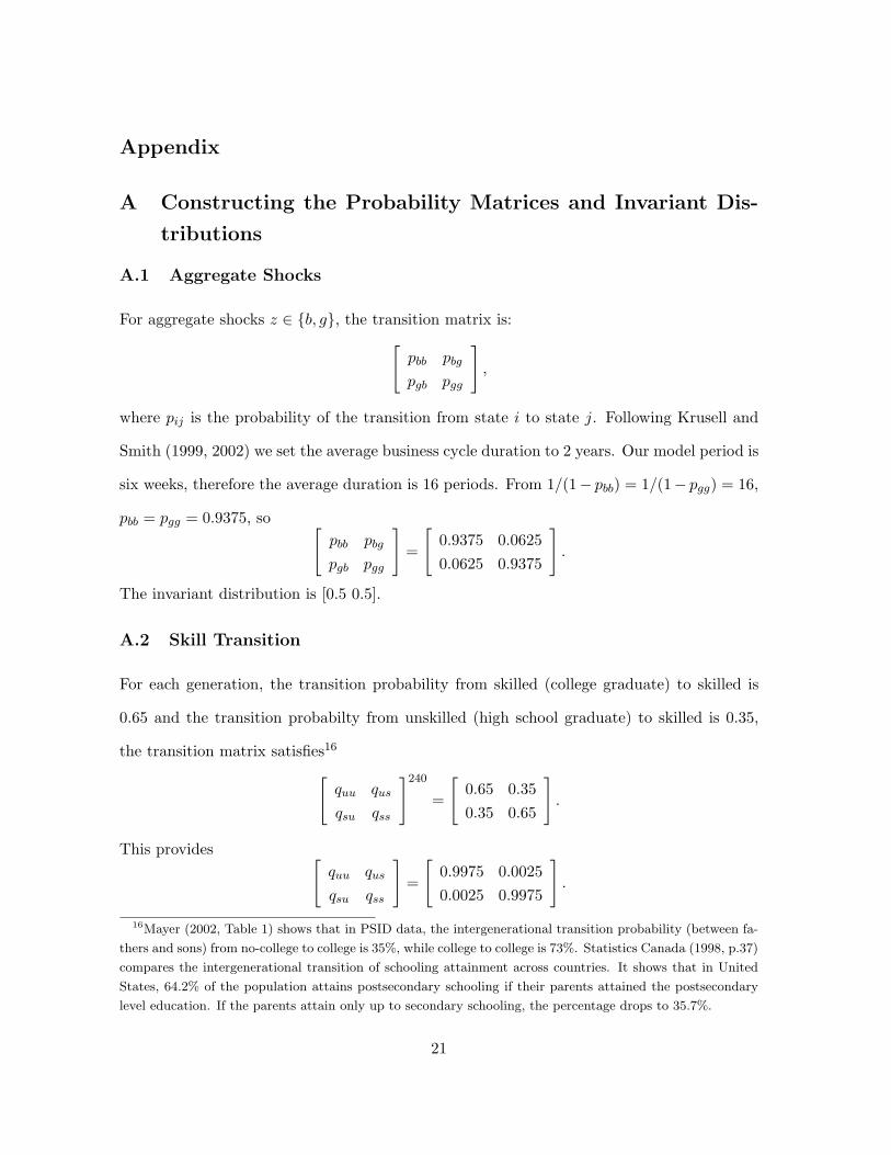
A.1 Aggregate Shocks

For aggregate shocks z ∈ b, g, the transition matrix is:[

pbb pbg

pgb pgg

],

where pij is the probability of the transition from state i to state j. Following Krusell and

Smith (1999, 2002) we set the average business cycle duration to 2 years. Our model period is

six weeks, therefore the average duration is 16 periods. From 1/(1− pbb) = 1/(1− pgg) = 16,

pbb = pgg = 0.9375, so [pbb pbg

pgb pgg

]=

[0.9375 0.06250.0625 0.9375

].

The invariant distribution is [0.5 0.5].

A.2 Skill Transition

For each generation, the transition probability from skilled (college graduate) to skilled is

0.65 and the transition probabilty from unskilled (high school graduate) to skilled is 0.35,

the transition matrix satisfies16

[quu qus

qsu qss

]240

=

[0.65 0.350.35 0.65

].

This provides [quu qus

qsu qss

]=

[0.9975 0.00250.0025 0.9975

].

16Mayer (2002, Table 1) shows that in PSID data, the intergenerational transition probability (between fa-

thers and sons) from no-college to college is 35%, while college to college is 73%. Statistics Canada (1998, p.37)

compares the intergenerational transition of schooling attainment across countries. It shows that in United

States, 64.2% of the population attains postsecondary schooling if their parents attained the postsecondary

level education. If the parents attain only up to secondary schooling, the percentage drops to 35.7%.

21

The invariant distribution is

[χu χs

]=

[0.5 0.5

].

Note that if we start from the invariant distribution, the fraction of skilled workers remains

constant by the law of large numbers.

A.3 Individual Shocks

For individual shocks ε ∈ 0, 1, the transition matrix has to be conditioned on last period’s

aggregate state (z), today’s aggregate state (z′), and today’s skill level (η′). Denote the

matrix as Πzz′η′ . Here the case z = b, z′ = b, and η′ = u is illustrated.

Πbbu =

[πbbu

00 πbbu01

πbbu10 πbbu

11

].

The unemployment rate of skill level η when the aggregate state is z is denoted as µzη. We

calibrate µzη from the Current Population Survey. Each year in between 1970 to 2001 is

divided into two categories (two equal numbers of good and bad years) by ranking the years

according to the total unemployment rate. µzη is given as the average unemployment rate of

the skilled and the unskilled for the good and the bad years.17

The number of people who were unskilled and unemployed in the last period is χuµbu.

They remain unskilled in the current period with probability quu. Thus, the number of people

who were unskilled and unemployed in the last period, and remain unskilled in the current

period is χuµbuquu. The amount of people who were skilled and unemployed in the last period

is χsµbs. They become unskilled in the current period with probability qsu. Thus, the amount

of people who were skilled and unemployed in the last period, and become unskilled in the

current period is χsµbsqsu. Summing up, the people who were unemployed in the last period

17The skilled are defined as some college or college completion, and the unskilled are defined as high school

completion or less. Since the population of each group changes over time, we took the weighted average of the

unemployment rates in each group using the number of individuals aged 24 and up (the population is taken

from the census data) at each year.

22

and unskilled in the current period is χuµbuquu + χsµ

bsqsu. The people who were employed in

the last period and unskilled in the current period is χu(1 − µbu)quu + χs(1 − µb

s)qsu. Thus,

as the transition occurs

[χuµb

uquu + χsµbsqsu χu(1− µb

u)quu + χs(1− µbs)qsu

] [πbbu

00 πbbu01

πbbu10 πbbu

11

]

=

[πbbu

00 χuµbuquu + πbbu

00 χsµbsqsu + πbbu

10 χu(1− µbu)quu + πbbu

10 χs(1− µbs)qsu

πbbu01 χuµb

uquu + πbbu01 χsµ

bsqsu + πbbu

11 χu(1− µbu)quu + πbbu

11 χs(1− µbs)qsu

]′.

Since the current period is a bad state, the first entry has to be equal to χuµbu. This provides

us with the first restriction. (The second entry has to be equal to χu(1− µbu), but it is easy

to show that this is automatically satisfied by the first restriction provided that χ is the

invariant distribution.) Now we have two unknowns, πbbu00 and πbbu

10 (the rest are determined

by the condition that the probabilities sum up to one: πbbu00 + πbbu

01 = 1 and πbbu10 + πbbu

11 = 1)

and one equation. Another restriction is provided from the unemployment duration data.

The Current Population Survey provides the average duration of unemployment in each

year. We calculated the average duration in the good years and in the bad years (defined by

the total unemployment rate), and obtained that the duration is 12.4 weeks for good years

and 15.9 weeks for bad years.18 Mincer (1991) shows (using PSID data) that the average

duration of unemployment is not significantly different between skilled and unskilled workers,

and therefore we use the same numbers for the skilled and the unskilled. The restriction is

1/(1− πbbu00 ) = 15.9/6. When selecting πbgη′

00 and πgbη′00 , there exist two approachs:

1. πbgη′00 = πggη′

00 and πgbη′00 = πbbη′

00 (Imrohoroglu [1989])

2. πbgη′00 = 0.75 · πggη′

00 and πgbη′00 = 1.25 · πbbη′

00 (Krusell and Smith [1999, 2002]).

We follow Krusell and Smith.

From the data on unemployment between 1970 and 2001 (described above), we calculate

µbu = 0.087, µg

u = 0.056, µbs = 0.038, and µg

s = 0.026.18Imrohoroglu (1989) uses the duration of 10 weeks in good times and 14 weeks in bad times. Krusell and

Smith (1999, 2002) use 19.5 weeks and 32.5 weeks.

23

Given above numbers, πbbu10 is derived from

πbbu10 =

χuµbu − πbbu

00 (χuµbuquu + χsµ

bsqsu)

χu(1− µbu)quu + χs(1− µb

s)qsu.

In general, πzz′η′10 is derived from

πzz′η′10 =

χη′µz′η′ − πzz′η′

00 (χuµzuquη′ + χsµ

zsqsη′)

χu(1− µzu)quη′ + χs(1− µz

s)qsη′.

The resulting Π matrices are:

Πbbu =

[0.6226 0.37740.0383 0.9617

],

Πgbu =

[0.7783 0.22170.0483 0.9517

],

Πbgu =

[0.3871 0.61290.0269 0.9731

],

Πggu =

[0.5161 0.48390.0309 0.9691

],

Πbbs =

[0.6226 0.37740.0152 0.9848

],

Πgbs =

[0.7783 0.22170.0184 0.9758

],

Πbgs =

[0.3871 0.61290.0123 0.9877

],

Πggs =

[0.5161 0.48390.0134 0.9866

].

A.4 Stochastic β

Following Krusell and Smith (1998), we assume that the discount factor βt follows a three-

point Markov stochastic process. Let βt ∈ l, m, h, where l < m < h. An agent with the

discount factor β = l is impatient, and an agent with the discount factor β = h is patient.

First, we calibrate the Markov transition matrix by imposing the following restrictions.

24

• 10% of the total population has β = l, 80% of the population has β = m, and 10% of

the population has β = h.

• There is no direct transition in between β = l and β = h.

• The average duration of the extreme states, β = l and β = h, is one generation (30

years).

The transition probabilities from state i to state j, ωij are

ωll ωlm ωlh

ωml ωmm ωmh

ωhl ωhm ωhh

=

239/240 1/240 01/1920 959/960 1/1920

0 1/240 239/240

.

Second, the values of βl, βm, βh are pinned down so that the resulting distribution of the

asset holdings mimics the real wealth distribution. In particular, βl = 0.992, βm = 0.995,

and βh = 0.998.

A.5 Skill Premium

In the model φ(s)/φ(u) is the skill premium. To calibrate φ(s)/φ(u) we use the estimates

of Murphy and Welch (1992). They compute the ratio of average wage of college graduate

workers to high-school graduate workers for different experience groups and for different

years. They find that this ratio, which can be interpreted as the skill premium, is between

1.37 to 1.58. To be consistent with their estimates, we set φ(s)/φ(u) to 1.50.

One can also calibrate φ(s)/φ(u) by using the estimates for return to college education.

If one assumes that the return to one year of college education is 10%, which is consistent

with the estimates in Card (1995), then φ(s)/φ(u) is around 1.50.

B Applying the “Integration Principle” to Idiosyncratic Shocks

Applying the “integration principle” to a two-point process is more difficult than the contin-

uous example in the main text. Here, starting from the static case, we extend the analysis

25

step by step.19

B.1 Static Case

Let z take two values, g and b, and ε take two values, 0 and 1. The aggregate state z occurs

with the probability πz(z), and ε’s probability depends only on the current z. The conditional

probability of ε given z is denoted as π(ε|z). We define i ∼ U(0, 1), and

g(i, z) =

1 if i ≤ π(1|z),0 otherwise.

Thus, when i ∈ [0, π(1|b)],

y =∑

z

g(i, z)πz(z) = g(i, g)πz(g) + g(i, b)πz(b) = 1 · πz(g) + 1 · πz(b) = 1.

When i ∈ (π(1|b), π(1|g)],

y = g(i, g)πz(g) + g(i, b)πz(b) = 1 · πz(g) + 0 · πz(b) = πz(g).

When i ∈ (π(1|g), 1],

y = g(i, g)πz(g) + g(i, b)πz(b) = 0 · πz(g) + 0 · πz(b) = 0.

In sum, y = 1 with probability π(1|b), y = πz(g) with probability π(1|g) − π(1|b), and

y = 0 with probability 1− π(1|g).

B.2 Correlation over Time

When z and ε are correlated over time, applying this procedure requires more thought.

Suppose that z evolves by a first-order Markov process and that εt depends on zt, zt−1, and

εt−1. Let it be an i.i.d. random variable which follows U [0, 1]. We must then find a function

g(·, ·) which satisfies

gt(ist0, zst

0) = gt(εst0, zst

0), (3)19For exposition, in this section we utilized slightly different notation from the main text. The correspon-

dence should be clear, however.

26

and then integrate gt(ist0, zst

0) over zst0. Note that the right hand side is the employ-

ment variable, gt(εst0, zst

0) = εt.

B.2.1 Brute-Force

One way to do this is by brute-force simulation: generate zt and it randomly, and then create

εt from the realization. Iterate the simulation many times – then, for each ist0, there will

be a distribution of εt (depending on the realizations (history) of z, ε can be different for the

same ist0). Average this out and use as the new idiosyncratic shocks at each t. We did not

utilize this method here.

B.2.2 Recursive

Instead, we utilized the following method, which exploits the recursive structure of the

problem. From the distributional assumptions, to express εt by an i.i.d. random variable

it ∼ U(0, 1), the additional information required is zt−1, zt, and εt−1. That is, given zt−1, zt,

and εt−1, εt can be determined by the rule

εt =

1 if it ≤ Ω(zt−1, zt, εt−1),0 otherwise,

(4)

where Ω(zt−1, zt, εt−1) is the threshold value calculated from the original Markov transition

matrices. However, we can not integrate this yet. Ω(zt−1, zt, εt−1) still depends on εt−1.

To construct gt(·, ·) function, we still require εt−1 to be expressed by i and z. By working

from t = 0 using (4) (ε−1 is given), we can express εt−1 by ist−10 , zst−1

0 . Clearly, this

procedure has recursive structure.

Equation (3) can be expressed as gt(it, zt, zt−1, εt−1) = εt, where εt−1 on the left hand side

is actually a function of ist−10 , zst−1

0 . The integration principle requires us to calculate,

for each ist0,

yt =∑zt

· · ·∑z0

gt(it, zt, zt−1, εt−1) · πz(zt, . . . , z0).

27

This can be rewritten as

yt =∑zt−1

· · ·∑z0

gt(it, g, zt−1, εt−1) · πz(g, zt−1 . . . , z0)

+∑zt−1

· · ·∑z0

gt(it, b, zt−1, εt−1) · πz(b, zt−1, . . . , z0).

The first part can be rewritten as∑zt−1

· · ·∑z0

gt(it, g, zt−1, εt−1) · πz(g, zt−1 . . . , z0)

=∑zt−2

· · ·∑z0

gt(it, g, g, εt−1) · πz(g, g, zt−2 . . . , z0)

+∑zt−2

· · ·∑z0

gt(it, g, b, εt−1) · πz(g, b, zt−2 . . . , z0).

(5)

The second part can be expressed in the similar way.

Let Pt−1(g, ε) be the probability that, for given ist−10 , the realization of zst−1

0 induces

(i) zt−1 = g and (ii) εt−1 = ε.

Further, let πz(zt|zt−1) be the conditional probability. Then, the first part of (5) can be

rewritten as:∑zt−2

· · ·∑z0

gt(it, g, g, εt−1) · πz(g, g, zt−2 . . . , z0)

= gt(it, g, g, 1) · πz(g|g) · Pt−1(g, 1) + gt(it, g, g, 0) · πz(g|g) · Pt−1(g, 0).(6)

Here, gt(it, g, g, 1) is either 0 or 1, and is easy to calculate using (4). πz(g|g) is given by the

Markov transition matrix. Thus, given Pt−1(zt−1, εt−1), yt can be calculated only from the

information of it, using (6) for all possible combinations of zt−1 and zt.

How can we get Pt−1(zt−1, εt−1)? It can be calculated recursively. First, notice that

Pt−1(zt−1, 0) + Pt−1(zt−1, 1) = πz(zt−1), where πz(zt−1) can be mechanically calculated from

the Markov transition matrix and the initial value z0. Thus, we only need to keep track of

Pt−1(zt−1, 1). To obtain Pt(g, 1), we have to calculate the probability of (i) zt = g and (ii)

εt = 1. This can be done by just picking up the zt = g part in the yt calculation (sum of

(6) for all possible combinations of zt−1 and zt), since gt(it, zt, zt−1, εt−1) = 1 if εt = 1 and

28

gt(it, zt, zt−1, εt−1) = 0 if εt = 0. That is,

Pt(g, 1) = gt(it, g, g, 1) · πz(g|g) · Pt−1(g, 1)+ gt(it, g, g, 0) · πz(g|g) · Pt−1(g, 0)+ gt(it, g, b, 1) · πz(g|b) · Pt−1(b, 1)+ gt(it, g, b, 0) · πz(g|b) · Pt−1(b, 0).

In the same way,

Pt(b, 1) = gt(it, b, g, 1) · πz(b|g) · Pt−1(g, 1)+ gt(it, b, g, 0) · πz(b|g) · Pt−1(g, 0)+ gt(it, b, b, 1) · πz(b|b) · Pt−1(b, 1)+ gt(it, b, b, 0) · πz(b|b) · Pt−1(b, 0).

Note that

yt = Pt(g, 1) + Pt(b, 1)

by construction. Up to this part, our procedure follows Krusell and Smith (2002).

B.3 Extending to Multiple Skill Levels

Suppose that the employment probability is also dependent on skill level η ∈ u, s, which

evolves stochastically. The evolution of η is first-order Markov, and independent of ε and z.

Specifically, yt(= εt) depends on εt−1, zt−1, zt, and ηt. Now, (4) has to be modified to20

εt =

1 if it ≤ Ω(zt−1, zt, εt−1, ηt),0 otherwise.

(7)

Here, εt−1 depends on ist−10 , ηst−1

0 , zst−10 . Clearly, after integration, y is a func-

tion of ist0, ηst

0. Similar steps from the previous case apply. Given ist0, ηst

0,

yt =∑zt

· · ·∑z0

gt(it, zt, zt−1, εt−1, ηt) · πz(zt, . . . , z0).

This can be rewritten as

yt =∑zt−1

· · ·∑z0

gt(it, g, zt−1, εt−1, ηt) · πz(g, zt−1 . . . , z0)

+∑zt−1

· · ·∑z0

gt(it, b, zt−1, εt−1, ηt) · πz(b, zt−1, . . . , z0).

20Clearly, Ω(zt−1, zt, εt−1, ηt) here should be set to πzt−1ztηt

εt−11 in the main text.

29

The first part can be rewritten as∑zt−1

· · ·∑z0

gt(it, g, zt−1, εt−1, ηt) · πz(g, zt−1 . . . , z0)

=∑zt−2

· · ·∑z0

gt(it, g, g, εt−1, ηt) · πz(g, g, zt−2 . . . , z0)

+∑zt−2

· · ·∑z0

gt(it, g, b, εt−1, ηt) · πz(g, b, zt−2 . . . , z0).

(8)

The second part can be expressed in a similar way.

Let Pt−1(g, ε) be the probability that, for given ist−10 , ηst−1

0 , the realization of

zst−10 induces (i) zt−1 = g and (ii) εt−1 = ε.

Further, let πz(zt|zt−1) be the conditional probability. Then, the first part of (8) can be

rewritten as:∑zt−2

· · ·∑z0

gt(it, g, g, εt−1, ηt) · πz(g, g, zt−2 . . . , z0)

= gt(it, g, g, 1, ηt) · πz(g|g) · Pt−1(g, 1) + gt(it, g, g, 0, ηt) · πz(g|g) · Pt−1(g, 0).(9)

Here, gt(it, g, g, 1, ηt) is either 0 or 1, and can be calculated by (7). πz(g|g) is given by the

Markov transition matrix. Thus, given Pt−1(zt−1, εt−1), yt can be calculated only from the

information of it and ηt, using (9) for all possible combinations of zt−1 and zt.

One could calculate Pt−1(zt−1, εt−1) recursively. First, notice that again Pt−1(zt−1, 0) +

Pt−1(zt−1, 1) = πz(zt−1), where πz(zt−1) can be mechanically calculated from the Markov

transition matrix and z0. Thus, we only need to keep track of Pt−1(zt−1, 1). To obtain

Pt(g, 1), we have to calculate the probability of (i) zt = g and (ii) εt = 1. This can be done by

just picking up the zt = g part in the yt calculation (sum of (9) for all possible combinations

of zt−1 and zt), since gt(it, zt, zt−1, εt−1, ηt) = 1 if εt = 1 and gt(it, zt, zt−1, εt−1, ηt) = 0 if

εt = 0. That is,

Pt(g, 1) = gt(it, g, g, 1, ηt) · πz(g|g) · Pt−1(g, 1)+ gt(it, g, g, 0, ηt) · πz(g|g) · Pt−1(g, 0)+ gt(it, g, b, 1, ηt) · πz(g|b) · Pt−1(b, 1)+ gt(it, g, b, 0, ηt) · πz(g|b) · Pt−1(b, 0).

(10)

30

In the same way,

Pt(b, 1) = gt(it, b, g, 1, ηt) · πz(b|g) · Pt−1(g, 1)+ gt(it, b, g, 0, ηt) · πz(b|g) · Pt−1(g, 0)+ gt(it, b, b, 1, ηt) · πz(b|b) · Pt−1(b, 1)+ gt(it, b, b, 0, ηt) · πz(b|b) · Pt−1(b, 0).

(11)

Note that

yt = Pt(g, 1) + Pt(b, 1)

by construction.

B.4 Algorithm

Denote the last period with aggregate fluctuations as t = 0.

1. For each agent, given z0, ε0, and η0, simulate it and ηt, and thus obtain the sequence

of Pt for t = 1, 2, .... Sum up and obtain the aggregate labor supply nt at t = 1, 2, ....

Check when nt and the distribution of the labor supply settles down. Call that period

N1. (We used N1 = 40 to 100, depending on the starting point.) From the process of

Pt, we can obtain the time series of y. Instead of using Pt in the individual decision

problem, we approximate this process of y by a finite-state Markov process and use

this as the individual shocks.

2. Pick N2 > N1. (We used N2 = 1000.) Use the average of the law of motions in t < 0

to guess kt, t = 1, 2, ..., N2. Call them k0t .

3. Given the law of motion for k and the stationary value of nt, perform the value-function

iteration (part of Krusell-Smith’s [1998] method) to obtain the value function for the

periods t = N1 + 1, ..., N2. Note that the decision problem is

V (k, y, η, β; k) = maxc,k′

log c + βE

[V (k′, y′, η′, β′; k′) |y, η, β

]

subject to

c + k′ = rk + wφ(η)y + (1− δ)k,

31

k′ = H(k),

k′ ≥ k,

r and w calculated from n and k.

4. From t = N1, work backwards to obtain value functions and decision rules for t =

1, ..., N1.

VN1(k, y, η, β) = maxc,k′

log c + βE

[V (k′, y′, η′, β′; kN1+1) |y, η, β

]

subject to

c + k′ = rk + wφ(η)y + (1− δ)k,

k′ ≥ k,

r and w calculated from nN1 and k0N1

.

5. Simulate the economy from t = 0, using the initial distribution at t = 0 and the decision

rules obtained above.

6. Compare the simulated path of k and k0. If they are not close enough, update the

k sequence by the weighted average. Also obtain the new prediction rule for k by

performing OLS for the new kt, t = N1, ..., N2.

C How to Find the Welfare Cost

The welfare cost from business cycles is defined (following Lucas) as λ which satisfies

E0

∞∑

t=0

(t∏

j=0

βj)U((1 + λ)cot )

= E0

∞∑

t=0

(t∏

j=0

βj)U(cst )

,

where cot∞t=0 is the consumption stream in the original economy (with business cycles), and

cst∞t=0 is the consumption stream in the “smoothed” economy (without business cycles).

32

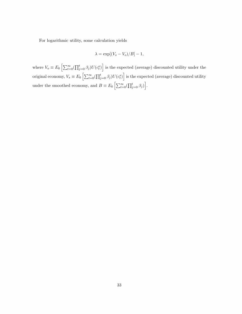
For logarithmic utility, some calculation yields

λ = exp[(Vs − Vo)/B]− 1,

where Vo ≡ E0

[∑∞t=0(

∏tj=0 βj)U(co

t )]

is the expected (average) discounted utility under the

original economy, Vs ≡ E0

[∑∞t=0(

∏tj=0 βj)U(cs

t )]

is the expected (average) discounted utility

under the smoothed economy, and B ≡ E0

[∑∞t=0(

∏tj=0 βj)

].

33

D More Tables

asset levelconstrained bottom 1% 50% 99% 99.9%

η = u, ε = 0 0.172% 0.087% -0.010% 0.003% 0.146%

η = u, ε = 1 0.139% 0.112% 0.039% 0.019% 0.156%

η = s, ε = 0 0.064% 0.004% -0.075% 0.031% 0.109%

η = s, ε = 1 0.038% 0.026% -0.010% 0.057% 0.126%

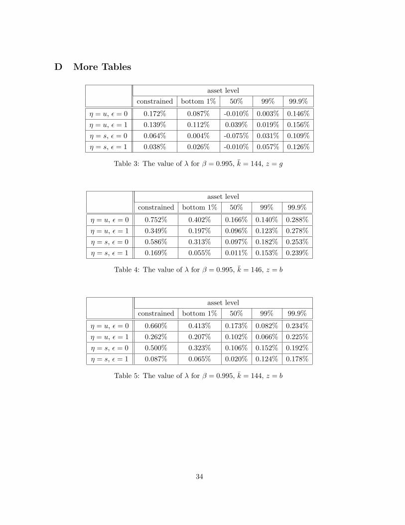
Table 3: The value of λ for β = 0.995, k = 144, z = g

asset levelconstrained bottom 1% 50% 99% 99.9%

η = u, ε = 0 0.752% 0.402% 0.166% 0.140% 0.288%

η = u, ε = 1 0.349% 0.197% 0.096% 0.123% 0.278%

η = s, ε = 0 0.586% 0.313% 0.097% 0.182% 0.253%

η = s, ε = 1 0.169% 0.055% 0.011% 0.153% 0.239%

Table 4: The value of λ for β = 0.995, k = 146, z = b

asset levelconstrained bottom 1% 50% 99% 99.9%

η = u, ε = 0 0.660% 0.413% 0.173% 0.082% 0.234%

η = u, ε = 1 0.262% 0.207% 0.102% 0.066% 0.225%

η = s, ε = 0 0.500% 0.323% 0.106% 0.152% 0.192%

η = s, ε = 1 0.087% 0.065% 0.020% 0.124% 0.178%

Table 5: The value of λ for β = 0.995, k = 144, z = b

34

References

[1] Aiyagari, S. Rao (1994). “Uninsured Idiosyncratic Risk and Aggrigate Saving,” Quarterly

Journal of Economics 109, 659–684.

[2] Atkeson, Andrew and Christopher Phelan (1994). “Reconsidering the Costs of Business

Cycles with Incomplete Markets,” in Stanley Fischer and Julio J. Rotemberg, eds., NBER

Macroeconomics Annual 1994, National Bureau of Economic Research.

[3] Barlevy, Gadi (2002). “The Cost of Business Cycles under Endogenous Growth,” mimeo.

Northwestern University.

[4] Belzil, Christian and Jorgen Hansen (2003). “Structural Estimates of the Intergenera-

tional Education Correlation,” Journal of Applied Econometrics 18, 679–696.

[5] Burdıa Rodrıguez, Santiago; Javier Dıaz-Gimenez; Vincenzo Quadrini; and Jose-Victor

Rıos-Rull (2002). “Updated Facts on the U.S. Distributions of Earnings, Income, and

Wealth,” Federal Reserve Bank of Minneapolis Quarterly Review 26, 2–35.

[6] Card, David (1995). “Earnings, Schooling, and Ability Revisited.” In Solomon Polachek,

ed., Research in Labor Economics Vol. 14. JAI Press: Greenwich Connecticut.

[7] Hansen, Gary D. and Ayse Imrohoroglu (1992). “The Role of Unemployment Insurance in

an Economy with Liquidity Constraints and Moral Hazard,” Journal of Political Economy

100, 118–142.

[8] Imrohoroglu, Ayse (1989). “The Cost of Business Cycles with Indivisibilities and Liquidity

Constraints,” Journal of Political Economy 97, 1364-1383.

[9] Keane, Michael and Eswar Prasad (1993). “Skill Levels and the Cyclical Variability of

Employment, Hours, and Wages,” IMF Staff Papers 40, 711–743.

35

[10] Krusell, Per and Anthony A. Smith, Jr. (1998). “Income and Wealth Heterogeneity in

the Macroeconomy,” Journal of Political Economy 106, 867-896.

[11] Krusell, Per and Anthony A. Smith, Jr. (1999). “On the Welfare Effects of Eliminating

Business Cycles,” Review of Economic Dynamics 2, 245-272.

[12] Krusell, Per and Anthony A. Smith, Jr. (2002). “Revisiting the Welfare Effects of Elimi-

nating Business Cycles,” mimeo. University of Rochester and Carnegie Mellon University.

[13] Lucas, Robert E. Jr. (1987). Models of Business Cycles, Basil Blackwell: New York.

[14] Lucas, Robert E. Jr. (2003). “Macroeconomic Priorities,” American Economic Review

93, 1–14.

[15] Mayer, Adalbert (2002). “Education, Self-Selection and Intergenerational Transmission

of Abilities,” mimeo. University of Rochester.

[16] Mincer, Jacob (1991). “Education and Unemployment,” NBER Working Paper, #3838.

[17] Murphy, Kevin M., and Finis Welch (1992). “The Structure of Wages,” Quarterly Jour-

nal of Economics 107, 285-326.

[18] Obstfeld, Maurice (1994). “Evaluating Risky Consumption Paths: The Role of Intertem-

poral Substitutability,” European Economic Review 38, 1471-86.

[19] Raisian, John (1983). “Contracts, Job Experience, and Cyclical Labor Market Adjust-

ments,” Journal of Labor Economics 1, 152–170.

[20] Statistics Canada (1998). Education Quarterly Review Vol.5, no.2.

[21] Topel, Robert (1993). “What Have We Learned from Empirical Studies of Unemploy-

ment and Turnover?” American Economic Review 83, 110-115.

[22] Wolff, Edward N. (1995). Top Heavy, The New Press: New York.

36