1

HETEROGENEITY IN THE WAGE IMPACTS OF

IMMIGRANTS

Priscillia E. Hunt

CSGR Working Paper 242/08

January 2008

2

Heterogeneity in the Wage Impacts of Immigrants

Priscillia E. Hunt

January 2008

Email: Priscillia.Hunt@Warwick.ac.uk

Abstract

This paper analyses impacts of immigration on individual wages. The empirical

analysis is based on the British Labour Force Survey from 1993 to 2005. In

addition to mean regression methods, this paper applies a semi-parametric

procedure to measure covariates at quantiles of the wage distribution. Results

indicate the substitutability of immigrant workers depends on the combination of

education and experience attained. Our main finding is university educated

immigrants with the least experience expand wages of all UK-born workers. We

also find positive wage impacts between workers with the same skill sets and

these effects are stronger for immigrants than natives.

JEL Classifications: J31, J61, C33

Keywords: Immigration, wage impacts, quantile regression

3

1. Introduction

According to the International Migration report1 for 2005, the foreign-born

comprised 9.1% of the United Kingdom's population. Compared to Western

Europe or the United States, the UK has a relatively low immigrant population

(11.9% and 12.9% respectively). Regarding nations of Europe, the migrant

stock2, as a percentage of the population, was greater in France (10.7%),

Germany (12.3%), Ireland (14.1%), Spain (11.1%) and Sweden (12.4%). On the

other hand, Britain maintained a larger proportion of immigrants than Greece

(8.8%), Italy (4.3%), Norway (7.4%), and Portugal (7.3%). Although there is a

moderate stock of migrants in the UK, the rate of growth of foreign-born in Britain

has increased considerably. The overseas-born as a percentage of the UK

population, through 1951 to 1991, grew at rates ranging from 0.46 to 0.87% per

decade.3 Through 1991-2001, the rate jumped to 1.64%. Most recently, 2000-

2005, the annual growth rate of foreign-born as a percentage of the UK

population was 2.3%. The UK growth rate of foreign-born was greater than

France (1.0%) and Italy (2.1%), but lower than Germany (2.7%), Ireland (9.8%),

and Spain (10%). The increasing rate at which immigrants are entering the UK

causes concern for academics, policy-makers, and the general public, as they

seek to determine the changes immigrants have on life in Britain.

Immigration has changed the profile of Britain's labour market. Unlike other

countries, such as the United States, immigrants to the United Kingdom have

relatively more education than natives. In Table 1, we illustrate the proportion of

immigrants and natives within particular education groups. Immigrants and

natives have roughly the same proportions, 21% and 17% respectively, in the

middle education group (leaving age of 17-18yrs). Interestingly, there are stark

differences in the lower and higher education groups. 36.2% of immigrants are in

the lowest education group (leaving age of 16 yrs or less) and 65.5% of natives

1United Nation's Department of Economic and Social Affairs, Population Division, 2006.

2Mid-year estimate of the number of people living in one country who are born

outside the country.3

Censuses, Office for National Statistics; General Register Office for Scotland; Northern IrelandStatistics and Research Agency

4

are in this lowest education group. Roughly 18% of natives and 43% of

immigrants are in the highest education group (leaving age of 19+ yrs).

Table 1: Educational Attainment Distribution

UK-born NonUK-born

Less than 17yrs 0.655 0.363

17-18 yrs 0.169 0.209

19+ yrs 0.176 0.428

Source: Author's LFS sample, 1993-2005. Employed males only.

The educational attainment of immigrants has been changing over the years. By

grouping immigrants into 5-year cohorts (based on year of entry into the UK), we

observe a gradual decline in entrants leaving education before 17 years of age.

The entrants leaving education after 18 years old has been increasing over time,

whilst the immigrants leaving between 17 and 18 years of age has remained

constant (see Figure 1).

Figure 1: Educational Attainment of NonUK-born Workers, by cohort of entry

0.00

0.10

0.20

0.30

0.40

0.50

0.60

0.70

pre5

5

56-6

0

61-6

5

66-7

0

71-7

5

76-8

0

81-8

5

86-9

0

91-9

5

96-0

0

01-0

5

Immigrant Cohort Groups

Fre

qu

en

cy

Less than

17yrs

17-18 yrs

19+ yrs

Source: Author's LFS sample, 1993-2005. Employed males only.

In summary, the proportion of immigrants was increasing and their skills were

changing, so we anticipate impacts on the labour market. Overseas-born workers

may improve wages for some UK-born workers and harm others, potentially

causing wage inequalities. In order to suggest whether immigrants were `good' or

`bad' for the economy, it is necessary to make judgments about the ranking of

5

importance for particular outcomes. Of course, this is not the work of economist

but for politicians and the voting public. To improve their decision-making

process, however, we seek to shed light on the issue of wage inequality. The

result has sociological and economic implications that we hope will enrich the

immigration debate of Britain.

The remainder of this paper is organised as follows. Section 2 surveys prior

literature analysing wage impacts of immigrants. Section 3 discusses the

theoretical framework and Section 4 introduces our data set. Section 5 develops

empirical strategies employed throughout the paper. Section 6 presents the main

results and the final section concludes with policy implications and areas for

further research.

2. Literature

The economic investigation of immigrant impacts is a growing body of work

reporting how the labour market functions with differentiated labour inputs. In

their detailed survey, Gaston and Nelson (2001) show that area studies and

factor proportions analysis typifies the labour market approach. Area analyses

find the change in earnings from a change in immigration within a particular

geographical area, whilst factor proportions approach examines how alterations

of the skill distribution leads to native outcome changes. Gaston and Nelson

(2001) suggest that the main issue for a researcher involved in either type of

investigation is to discern an accurate level of analysis. Both natives and

immigrants make location decisions and it may not be entirely clear what

geographical boundaries to select. Several authors (Filer (1992), Borjas (1997),

Frey (1995), Card and Dinardo (2000), Hatton and Tani (2005)) find mixed results

regarding the relationship between native migration patterns and immigration

rates. It is generally understood, however, the greater the area of analysis, the

less possibility of biased results because mobility is more fully accounted. We

model individual wages in the national labour market and control for region of

inhabitance, which accounts for any general equilibrium effects in terms of

mobility.

6

In a comparison of the area and factor proportions approaches, Borjas, Freeman,

and Katz (1996) detect effects of the immigrant-to-native ratio on the supply of

native labour and native wages in the relevant region. Using 1980 and 1990

Public Use Microdata Sample (PUMS) US Census data and Current Population

Survey (CPS), Borjas et al. (1996) discover that the greater the geographical

region, the less positive or more negative becomes the immigrant impact. This is

because when the geographical region under investigation is too small, it does

not factor in the location decisions of natives and exaggerates the immigrant

supply in the immigrant-to-natives ratio. Borjas et al. (1996) conclude that

immigrants and trade had the most depressive effect, -.039 log points, on relative

weekly wages of high school dropouts to other workers and -0.016 points for

log(high-school/college equivalents).

Two well cited area studies are Card (1990) and Friedberg (2001) looking at the

US and Israel, respectively. Card (1990) exploits the Mariel Boatlift operation in

which Cubans were granted permission to immigrate and increased the

population of Miami, Florida by nearly 7%. Card (1990) found no effect on wages

or employment on non-Cuban workers.4 Friedberg (2001) investigates the 1990-

1994 emigrations from the Soviet Union into Israel, which increased Israel's

population by 12%. OLS regressions indicate a depressive wage and

employment effect, but IV regressions suggest immigrants were in occupations of

falling wages already and there was no evidence immigrants impacted wages.

There is some work investigating the periods of EU enlargement to uncover

immigrant impacts. Portes and French (2005) evaluate unemployment changes in

Britain from the introduction of the European free movement of workers. They

use Worker Registration Services data and Social Insurance administration data

for the UK from 2003 through 2004. They find significant results in their

unrestricted OLS and an OLS on agriculture and fishing registrations only. Their

4Angrist and Krueger (1999) provide evidence contradicting Card's results.}

7

main finding is there are higher unemployment rates amongst natives in the local

authorities with greater immigration, albeit very small. These rates of

unemployment are mean reverting, and the speed of mean reversion increases

the further away it travels. They suggest the mean reversion is due to relatively

flexible labour market of the UK, welfare-to-work intervention, and/or mobility of

factors of production. In another work using the change in labour market

openness, Blanchflower, Saleheen, and Shaforth (2007) evaluate the impact of

the flow of A8 European Union enlargement workers into Britain. They examine

relationships between unemployment rates and other structural developments

across regions. The basic theoretical framework is immigrants are consumers

and producers so they affect both aggregate supply and demand. Consequently,

there is a relative change in demand and supply. Plus, the natural rate of

unemployment declines when the proportion of individuals in the population with

high propensities for unemployment declines. Blanchflower et al. (2007) find A8

immigration increased supply more than demand, but it also increased labour

market flexibility and likely lowered the natural rate of unemployment and the

NAIRU.

There are few immigrant population shocks like that found in Card (1990) and

Friedberg (2001), thus researchers make use of empirical strategies to uncover

immigrant impacts. Borjas (2003) developed a new framework to directly examine

the impact of immigration. In effect, he constructs `skill cells', which are

combinations in the levels of education and experience. His approach allows

workers with the same education but different levels of work experience to be

imperfect substitutes. Borjas's (2003) findings are consistent with competitive

labour market theory, where immigrants reduce wages of competing natives.

Interestingly, however, Borjas (2003) finds college graduate immigrants have a

positive effect on similarly educated natives and argues this may be due to

changing wage structure. Since he is unable to control for experience-period

interactions, the positive coefficient is most likely the result of increasing returns

to education for the highest education group. This result is consistent with Card

8

and Lemieux's (2001) findings that returns to education for those in the highest

education group have been increasing relative to other education groups.

A recent work by Ottaviano and Peri (2006) stresses the importance of the

general equilibrium framework and argues that estimates should take skill

distribution and substitutability into account. Building on Borjas's (2003) strategy

of education and experience determining skill groups, Ottaviano and Peri (2006)

derive the demand for differentiated labour from a CES production function and

generate measures of immigrant impacts. They use the integrated Public Use

Microdata Samples (IPUMS) of the US Census to study impacts of immigration

from 1980-2000. Ottaviano and Peri (2006) conclude the overall wage impact of

immigration was a 2.0-2.2% with the least positive, potentially negative, impact

on the lowest education group. Following Ottaviano and Peri's (2006) technique,

Manacorda, Manning, and Wadsworth (2006) use the British General Household

Survey (GHS) and LFS to estimate a CES production function and assess

changes to the wage structure. Their main finding is immigrants do not effectively

compete with natives in wages. Manacorda et al. (2006) argue the wages of

native-born workers relative to immigrants can vary over time even with fixed

levels of demand and supply. The methodology uses observed wage bill shares

and estimated elasticities of substitution to compute the changes in wages for

each cell in response to different hypothetical changes in the number and

composition of immigrants. This specific framework was developed in Ottaviano

and Peri (2006), which itself is an augmented version of the modelling strategy in

Borjas (2003). Imperfect substitutability is permitted to arise from different

abilities, occupational choices, or unobserved characteristics of workers.

Manacorda et al. (2006) find the rise in immigration has changed Britain's wage

structure. Immigration has depressed the earnings of immigrants relative to

native-born. Since immigrants had relatively more university education than

natives and returns to education are sensitive to the relative supply of university

graduates (Card and Lemieux (2001)), there would be an effect on both migrants

and natives. Since the immigrant share is relatively low, the size of the effect on

natives, they argue, is negligible.

9

In the first endeavour to estimate wage and employment impacts from immigrants

into Britain, Dustmann, Fabbri, and Preston (2005) use the British Labour Force

Survey (LFS) to determine employment, unemployment, participation, and wages

effects on 17 UK regions for the period 1983-2000. They estimate OLS,

Difference, and IV-Difference models for outcomes of a region using a ratio of

immigrant to natives to determine effects. In order to account for native

responses and identify the model, they include a vector of natives' skills.

Dustmann et al. (2005) do not find statistically significant impacts of immigrants

on regional outcomes. Although when they group natives by education group,

they do find weakly determined results on the intermediate level. There is a 17.9

percent reduction in employment, 9.8 percent increase in unemployment, 10.8

percent decrease in participation; wages were insignificant, but they find a 15.3

increase for natives. This paper produces some puzzling results. According to the

factor price equalisation theory that they state as their theoretical framework,

when the skill distribution of natives is unlike that for immigrants a wage effect

should occur. So even though immigrants tend to have more education and

returns to education are sensitive at higher levels (Card and Lemieux (2001)),

they find no effect on natives' earnings.

There are several methodological strategies a researcher can choose to extract

information about immigrant effects. The spatial correlations method evaluates

average regional wage changes over time and exploits geographical differences

in immigrant settlement to find for impacts. Natural experiment approach

compares affected and unaffected regions of immigrant flow shocks to make an

impact assessment. One last methodology, simulations methods, calculates the

impact of variations in the quantities of factors of production on their prices. One

feature is similar in all of these methodologies; they focus on mean aggregate

outcomes. Koekner and Hallock (2001) suggest that empirical economics is well

justified to concentrate on the tails of the distribution. Tannuri-Pianto (2002)

performs, to our knowledge, the first and only quantile regression focusing on

immigrants to determine effects across the wage distribution. She uses Machado

10

and Mata's (2005) method to decompose changes in native-immigrant skills and

changes in the return to skills in the United States over the period 1970-1990.

The technique allows Tannuri-Pianto (2002) to perform a counterfactual analysis

to suggest what would have happened if the distribution of explanatory variables

had remained as in a previous period. It appears natives' earnings grew relative

to immigrants from 1970 to 1990 because of differing effects of return to skills for

natives and changing workers' characteristics. However, the changing wages

structure, which harmed low and middle-income immigrants more than natives

and improved high-income immigrants more than natives, diminished the wage

gap. A potential weakness is this approach does not take into account any

general equilibrium effects. We also perform quantile regressions, as a

robustness check on the mean regression estimates.

3. Theory

In the simplest of frameworks, equating the supply and demand for labour and

setting prices at marginal cost determine wages and output. The price of marginal

productivity from labour is the wage; hence, increasing an individuals' productivity

(i.e. further education, more experience) increases their wage. This is the crux of

human capital theory formalised by Becker (1975). However, employers cannot

observe all productivity characteristics, so they reward personal characteristics

that proxy for productive attributes. For example, marital status suggests

dependability or loyalty, which is positively rewarded in the labour market.

Therefore, we can estimate a wage received by an individual as a function of his

or her personal and productive characteristics, such as work experience and

education. Mincer (1974) initiated this line of work to estimate the schooling

premium in which log earnings are regressed on years of education to determine

the returns to education5.

Immigration has implications for the productivity of an individual and thus, his or

her wages. Foreign-born workers bring knowledge and creativity from differing

5Heckman, Lochner, and Todd (2005) argue this type of estimation is actually the price of

schooling in a hedonic market wage equation and not an internal rate of return to education.

11

systems, which may improve the ability of native workers to do their job. A basic

analysis suggests immigrant workers are a labour supply shock, which shifts the

supply curve out and exerts downward pressure on wages. However, this

relationship between price and quantity of labour only exists when immigrants

substitute for native labour. Immigrants can expand the productivity of native

workers and increase returns to labour. This indicates complementarity, which

leads to upward pressure on wages. Differing skill sets between immigrants and

natives is the key factor in determining how immigrants affect native productivity

(wages), so we will define our foreign variables of interest as ratios of immigrants-

to-natives. Specifically, the variables will be ratios of immigrants-to-natives

possessing the same skill set of education and experience. Categories of skill are

the basis for competitiveness and thus, a channel through which immigrants

affect native wages. In order to determine what groups of immigrants exert

upward or downward pressure on native wages, it is essential to explain the

definition of 'skills'. We derive skill categories, or cells, from the combinations of

education levels and years of experience in a fashion similar to Borjas (2003).

This allows us to calculate which immigrants increase, decrease, or have a null

effect on native wages. If immigrants increase natives' productivity, we will find

for a positive coefficient on our foreign variable in the wage equation. This is

consistent with immigrants acting as complements to natives in production. In

contrast, if immigrants are substitutes, we will observe a negative coefficient on

the immigrant skill category. Temporal variation of immigrant-native skill ratios

provides an opportunity to examine how foreign workers absorb into the British

labour market.

The substitutability of immigrants to natives depends not only on observable

skills, but unobservable factors as well and estimating an overall wage impact

may be misleading. Some natives will find themselves better off, whilst others are

harmed. Specifically, we determine how immigrants influence wages of low- to

high-ability individuals through the quantile regression (QR) technique. A quantile

regression calculates coefficients based on least absolute deviation from the

quantile, or percentile, of interest. Thus, we can loosen restrictions on the error

12

term and estimate coefficients for groups of individuals with low- and high-

unobservables separately. The quantile analysis ensures OLS estimates capture

the true effect of immigrants and unobserved heterogeneity is not driving our

findings. In addition, we can make statements about the effect of immigrants on

natives with particular abilities and form conclusions about immigrant impacts on

wage inequality.

4. Data

The British Labour Force Survey (LFS) is based on a systematic random sample

design, which makes it representative of the entire UK. An LFS year is composed

of four seasonal-quarters: Spring (March-May), Summer (June-August), Autumn

(September-November), and Winter (December-February). Each quarter

samples 125,000 individuals from approximately 60,000 households. Not all

questions are posed to a household at once. The questions are posed over five

successive quarters, which are called 'waves'. Therefore, in each quarter 12,000

households are in their wave 1, 12,000 are in wave 2, etc. The LFS is released

quarterly and there are variables indicating the interviewee's wave, as well as the

quarter and year the individual entered the survey. Quarters of the LFS were

seasonal until January 2006; the survey was then switched to calendar-quarters

in order to fulfil European Union regulations. The survey has been carried out

annually in its current form since 19836; however, earnings information is only

available since 1992. The earnings question is asked in wave 5 from 1992

onwards and then also in wave 1 from 1997 onwards. For consistency, we use

wave 5 wages whenever possible. We only use wave 1 earnings for those

persons with positive wages in wave 1 and non-response in wave 5. When we

inflate wages, we use the index corresponding to the year and quarter when the

respondent gave their earnings details.7 Wages are reported in terms of weekly

earnings, so we derive hourly wages by dividing (gross) weekly earnings into

weekly hours worked. To account for inflation and determine real wages, we use

6The LFS was carried out on a biennial basis from 1973 to 1983.

7We do not use the year and quarter in the survey because that relates to the period in which the

respondent entered the survey.

13

the UK Retail Price Index8 (RPI). We use 2005Q4 prices as the base period to

inflate all prior earnings observations. We pool cross-sections of the LFS from

1993Q1 to 2005Q4. The data used for this estimation includes men aged 16-64

in full-time employment. Earnings are not reported for the self-employed.

Quantile regression estimates are simultaneously estimated for quintiles- .10,

.25, .50, .75, .90- using Stata 9.2.

4.a. Summary Statistics

In Table 2, we present a summary of statistics characterising the sample we use

for wage analysis. The data is from 1993 to 2005 and descriptive statistics are

aggregated data of individual level responses from the LFS data set. Results

show that foreign-born workers earn more than UK-born, £12.18 and £11.05

respectively. Foreign-born workers are on average the same age as native

workers, roughly 38 years old. Average age at immigration is 19 years old and

average years in the UK are 20 years. There are significantly more non-whites in

the immigrant population than in the native population. Less than 2% of working

age, employed males born in the UK are non-white, whilst 39% of the immigrant

workforce is non-white. The geographical dispersion of UK-born workers is much

greater for natives than immigrants. The greatest regional concentration of UK-

born working males is in the South East (21%), 2-9% concentration in the other

regions of England, and 10% living in Scotland. Immigrants, on the other hand,

are highly concentrated in London (33%) and the South East (23%). Roughly the

same proportion of natives and immigrants are married or living together as a

couple, 50% and 54% respectively.

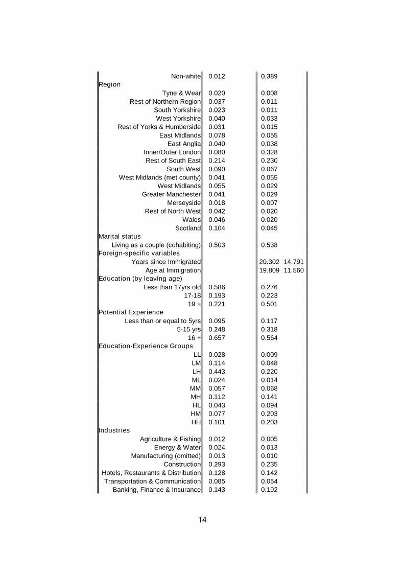
Table 2: Summary Statistics, 1993-2005

UK-born NonUK-bornVariable

Mean SD Mean SD

Dependent variable

Log of gross real hourly pay 2.403 0.549 2.500 0.585Independent variable

Age 38.839 11.141 38.588 10.392

Race

8From the Office of National Statistics.

http://www.statistics.gov.uk/StatBase/tsdataset.asp?vlnk=7173

14

Non-white 0.012 0.389Region

Tyne & Wear 0.020 0.008

Rest of Northern Region 0.037 0.011

South Yorkshire 0.023 0.011

West Yorkshire 0.040 0.033

Rest of Yorks & Humberside 0.031 0.015

East Midlands 0.078 0.055

East Anglia 0.040 0.038

Inner/Outer London 0.080 0.328

Rest of South East 0.214 0.230

South West 0.090 0.067

West Midlands (met county) 0.041 0.055

West Midlands 0.055 0.029

Greater Manchester 0.041 0.029

Merseyside 0.018 0.007

Rest of North West 0.042 0.020

Wales 0.046 0.020

Scotland 0.104 0.045

Marital status

Living as a couple (cohabiting) 0.503 0.538Foreign-specific variables

Years since Immigrated 20.302 14.791

Age at Immigration 19.809 11.560Education (by leaving age)

Less than 17yrs old 0.586 0.276

17-18 0.193 0.223

19 + 0.221 0.501Potential Experience

Less than or equal to 5yrs 0.095 0.117

5-15 yrs 0.248 0.318

16 + 0.657 0.564Education-Experience Groups

LL 0.028 0.009

LM 0.114 0.048

LH 0.443 0.220

ML 0.024 0.014

MM 0.057 0.068

MH 0.112 0.141

HL 0.043 0.094

HM 0.077 0.203

HH 0.101 0.203Industries

Agriculture & Fishing 0.012 0.005

Energy & Water 0.024 0.013

Manufacturing (omitted) 0.013 0.010

Construction 0.293 0.235

Hotels, Restaurants & Distribution 0.128 0.142

Transportation & Communication 0.085 0.054

Banking, Finance & Insurance 0.143 0.192

15

Public admin, Education & Health 0.163 0.204

Other Services 0.138 0.145

N 130,558 8,282

Source: Author's LFS sample, 1993-2005. Employed males only.

Since we will use education and experience groups as the factor of

substitutability, we are particularly interested in differences between the foreign-

born and natives. Table 2 reports immigrants have relatively more workers

leaving education at 19 years old or later (50%) than natives (22%). Conversely,

natives are more concentrated (59%) in the lowest education group than natives

(28%). Immigrants and natives have similar proportions, 19% and 22%

respectively, in the middle education group of 17-18 years leaving age.

Regarding years of experience, immigrants have less overall than natives. Nearly

66% of natives are in the highest experience group, whilst 56% of immigrants are

within this category.

To observe any cohort education trends, we graph the proportions of immigrants

in each education category. We are interested to discover what, if any,

educational attainment differences there are between immigrants over time. As

can be seen in Figure 1, there has been a downward trend in the proportion of

low educated and an upward trend of highly educated immigrant workers. The

proportion of immigrants leaving school at 17 or 18 has been constant. It is

beyond the scope of this paper to suggest why this occurred, however, it would

be interesting to find what policies and/or economic relationships prompted this

trend.

We are interested to find out which occupations9 immigrants accept and whether

this is different from natives. In Figure 2 we illustrate the distribution of

occupations chosen by immigrants and natives with positions of authority

descending from left to right. One of the most noticeable differences is between

immigrants and natives in the skilled-trades. There are significantly larger

proportions of natives than immigrants in skilled-trades. Generally, immigrants

9See Appendix for LFS Occupation definitions.

16

are more smoothly distributed in occupations and more immigrants than natives

are in higher positions. We find there are relatively few differences in

occupational choice for natives and immigrants.

Figure 2: Occupational Distribution of British Labour Force, by nativity

0.00

0.05

0.10

0.15

0.20

0.25

Man

ager

s&

Senior O

fficials

Profe

ssiona

l Occ

upat

ions

Assoc

iate

Prof &

Tech

Admin

&Sec

reta

rial

Skille

dTr

ades

Perso

nal S

ervice

s

Sales

&Cus

tom

erSer

vice

Proce

ss, P

lant

&M

achine

Ope

rativ

es

Elem

enta

ryOcc

upat

ions

Occupations

Fre

qu

en

cy

UK-born

NonUK-

born

Source: Author's LFS sample, 1993-2005. Employed males only.

Immigrants may have lower reservation wages due to less alternative sources of

income or lack of borrowing options. This is important because if it leads to

immigrants accepting positions for which they are over-qualified, our skill

definition, education-experience, is an inaccurate term of comparison. Immigrants

and natives would not compete for jobs in terms of their education and

experience, but on some other definition of skill. In Table 3, we present immigrant

occupations within each of the education-experience cells. In essence, we cross-

tab occupations with skill groups and as Table 3 illustrates, we do not find

evidence of mismatching occupations to education-experience. Within the lower

skill cells, proportions to the Low-educated immigrants, of all experience levels,

are mostly involved in skilled-trades rather than other occupations. The bottom,

17

right-hand of Table 3 shows that highly educated immigrants are filling

professional roles rather than accepting positions for which they are over-

qualified. For example, nearly 61% of highly educated, mid- and highly-

experienced immigrants are in professional and managerial/senior roles.

Comparing this to natives, in Table 4, we find similar results. Natives are more

likely than immigrants of the same education-experience group to be in higher

occupations, but the differences are minor. There are some significant

differences in the lowest education-experience category, LL, in which LL

immigrants are more evenly distributed in Sales & Customer Service, Personal

Services, and Skilled Trades. There are 15% more LL natives than LL immigrants

in Skilled Trades. On the other end of the spectrum, HH natives are more likely

than HH immigrants to be Associate Professionals & Technicians, Professionals,

and Managers & Senior Officials. In regression estimates, we allow all education-

experience groups to affect an individual's wage and yet, we can see in Table 3

and Table 4 that LL immigrants are not competing for the same positions as HH

natives. For example, the lowest five occupations employ 10% of HH natives

whilst these occupations employ nearly 85% of LL immigrants and 85% of LL

natives. Therefore, it is more consistent with the descriptive evidence that HH

natives manage LL workers and do not compete with one another. This leads us

to believe there are immigrant skill share groups that do not substitute nor

complement through competition. Instead, the lowest skill cells work for the

highest skill cells. Coefficients on immigrant shares may be interpreted as the

productivity (wage) impact of immigrant compared to native employees.

Table 3: Occupational Distribution of Education-Experience Groups, Immigrants

LL LM LH ML MM MH HL HM HH

ElementaryOccupations 19.26% 17.20% 12.42% 22.26% 12.91% 7.90% 8.83% 6.08% 5.12%

Process, Plant &Machine Operatives 14.25% 19.15% 23.31% 8.70% 12.09% 12.35% 4.71% 4.96% 5.69%

Sales & CustomerService 13.98% 5.71% 3.39% 10.96% 6.56% 3.83% 7.13% 3.46% 2.76%

Personal Services 13.72% 12.46% 8.61% 14.96% 11.94% 6.87% 5.83% 4.65% 2.99%

Skilled Trades 23.22% 21.64% 22.46% 13.91% 14.40% 14.24% 4.90% 6.31% 6.16%

Admin & Secretarial 5.80% 5.90% 3.34% 12.52% 8.15% 6.38% 8.20% 5.00% 4.57%

18

Associate Prof &Tech 3.69% 5.59% 5.36% 8.70% 12.70% 12.46% 16.89% 14.03% 11.33%

ProfessionalOccupations 1.58% 1.58% 3.03% 2.09% 6.66% 9.14% 30.85% 31.91% 31.23%

Managers & SeniorOfficials 4.49% 10.76% 18.10% 5.91% 14.60% 26.82% 12.66% 23.62% 30.15%

Total 100.00% 100.00% 100.00% 100.00% 100.00% 100.00% 100.00% 100.00% 100.00%

Table 4: Occupational Distribution of Education-Experience Groups, UK-born

LL LM LH ML MM MH HL HM HH

ElementaryOccupations 19.81% 12.48% 10.08% 14.73% 6.02% 3.58% 5.60% 1.87% 0.98%

Process, Plant &Machine Operatives 13.62% 19.79% 19.85% 8.52% 8.87% 6.44% 2.99% 2.10% 1.79%

Sales & CustomerService 8.05% 5.10% 3.31% 15.12% 6.46% 3.89% 7.99% 2.98% 1.64%

Personal Services 5.09% 5.99% 4.79% 7.86% 7.35% 4.16% 4.48% 2.39% 1.21%

Skilled Trades 38.17% 31.02% 27.36% 17.86% 15.78% 11.44% 6.17% 5.57% 5.05%

Admin & Secretarial 7.93% 6.88% 4.51% 16.02% 11.25% 6.68% 12.74% 4.89% 2.77%

Associate Prof &Tech 3.76% 6.48% 7.46% 9.89% 16.61% 16.70% 20.56% 20.07% 14.20%

ProfessionalOccupations 1.28% 2.91% 4.93% 3.37% 7.90% 14.06% 26.47% 33.39% 40.74%

Managers & SeniorOfficials 2.29% 9.35% 17.72% 6.62% 19.76% 33.05% 12.99% 26.73% 31.61%

Total 100.00% 100.00% 100.00% 100.00% 100.00% 100.00% 100.00% 100.00% 100.00%Source: Author's LFS sample, 1993-2005. Employed males only.

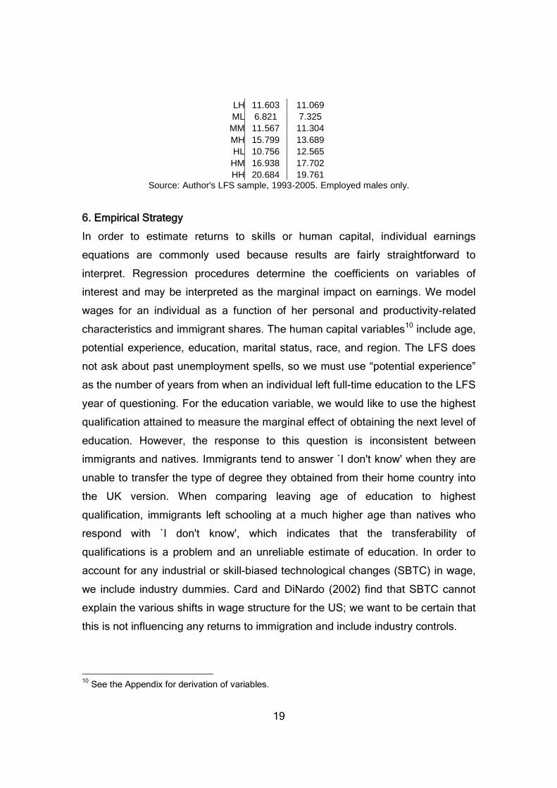
Table 5 demonstrates the average wages for UK- and NonUK-born workers in

each skill group. There are some significant differences in the wages between

UK- and NonUK-born of the same skill groups, although we are cautious about

the statistical validity of the descriptives because the number of immigrants in a

couple of the categories is very small. Nevertheless, we see that in the skill

groups of high-experience, with any level of education, immigrants earn less on

average than natives. In contrast, in groups with Low-experience and any level of

education, immigrants earn more on average than natives.

Table 5: Mean real wage of Education-Experience groups, by nativity

UK-bornNonUK-

born

LL 5.626 6.443

LM 9.639 9.023

19

LH 11.603 11.069

ML 6.821 7.325

MM 11.567 11.304

MH 15.799 13.689

HL 10.756 12.565

HM 16.938 17.702

HH 20.684 19.761Source: Author's LFS sample, 1993-2005. Employed males only.

6. Empirical Strategy

In order to estimate returns to skills or human capital, individual earnings

equations are commonly used because results are fairly straightforward to

interpret. Regression procedures determine the coefficients on variables of

interest and may be interpreted as the marginal impact on earnings. We model

wages for an individual as a function of her personal and productivity-related

characteristics and immigrant shares. The human capital variables10 include age,

potential experience, education, marital status, race, and region. The LFS does

not ask about past unemployment spells, so we must use “potential experience”

as the number of years from when an individual left full-time education to the LFS

year of questioning. For the education variable, we would like to use the highest

qualification attained to measure the marginal effect of obtaining the next level of

education. However, the response to this question is inconsistent between

immigrants and natives. Immigrants tend to answer `I don't know' when they are

unable to transfer the type of degree they obtained from their home country into

the UK version. When comparing leaving age of education to highest

qualification, immigrants left schooling at a much higher age than natives who

respond with `I don't know', which indicates that the transferability of

qualifications is a problem and an unreliable estimate of education. In order to

account for any industrial or skill-biased technological changes (SBTC) in wage,

we include industry dummies. Card and DiNardo (2002) find that SBTC cannot

explain the various shifts in wage structure for the US; we want to be certain that

this is not influencing any returns to immigration and include industry controls.

10See the Appendix for derivation of variables.

20

Similar to other works of immigrant impacts on wages (Borjas (2003), Dustmann

et al. (2005)), our foreign variables are ratios of immigrants to natives. We,

however, add an element in which the ratios are based on the same skill level.

The skill level is an interaction of education and potential experience. We

construct three categories of education indicating low (L), middle (M), and high

(H) levels of educational attainment. These are based on standard leaving ages

from education institutions: ≤16, 17-18, 19+. We construct three experience

groups in a similar fashion11, so we have low (L), middle (M), and high (H) with

the following years of potential experience: ≤5 years, 6-15 years, 16+years. We

then interact these two groups to construct nine education-experience dummies:

LL, LM, LH, ML, MM, MH, HL, HM, and HH. To detect immigrant impacts, we use

the ratios of immigrants to natives with the same skills combination (LL, LM, LH,

etc…). Since ratios in each skill cell change over time, we are able to calculate the

wage effect of a relative change in skills.

In Borjas (2003) and Dustmann et al. (2005), the left-hand side variable is the

mean outcome for native men within each skill cell of a particular region so that

wage equations are estimated separately for each education-experience group.

We, however, interact immigrant-native skill ratios with a vector of skill dummies

for natives. This produces different coefficients for natives of each education-

experience group and yet includes all information to estimate the rest of the

parameters. We consider this an attractive aspect of our procedure because we

are able to include more information, which generates more accurate coefficient

estimates. There is potential weakness in our estimation strategy where we have

not accounted for temporal variation in wages of skill groups. Since we utilise

repeated cross-sections and identify immigrant impacts for skill groups through

dummies, it may be necessary to control for time effects common to skill groups.

We consider this an avenue for improvement.

The model we are interested in estimating is:

11Although somewhat arbitrary, we consider the experience levels demanded by employers in job

offers.

21

yit = α + βxit + πmtj+uit ,

for i=1,…N, t=1,…T, j=LL, LM, LH,…HH, where yi is the real hourly wage for UK-

born individual i at time t, α is a constant of the mean national wage, xit is a vector

of personal characteristics (including potential experience, education, industry

dummies, etc.) for individual i at time t, mtj is the ratio of immigrants to natives

with education-experience combination j at time t, and uit is the error term. α, β,

and π are the parameters to be estimated.

When we perform the quantile regression, the model is specifically:

yit = αθ + βθxit + πθmtj+uθit. (1)

Since we control for personal attributes, productivity-related characteristics, and

cyclical and technological/industrial changes, the coefficient on the immigrant

variable, π, may be interpreted as the immigrant skill-group effect on the quantile

of interest. Performing a quantile regression produces within group effects.

Suppose πθ<0 for j=LL and θ=0.10, low-education/low-experience immigrants

substitute for low-ability natives. On the other hand, if πθ >0, then LL immigrants

are complements and the LL immigrants exert upward pressure on wages for

average native workers in the lowest quantile. Estimating equation (1) will

indicate whether transferability of immigrant skills affect wages of high-ability

natives dissimilarly from low-ability natives. Standard errors are estimated by

boostrapping with 20 resamples.

We also compare the immigrant effect between native education-experience

groups. To compare across skill groups, we introduce a dummy on the foreign

term in equation (1) and estimate:

yit = α + βxit + γ(mtj*Di)+uit. (2)

The foreign variable of interest here is the interaction term of the vector of skill-

group immigrant shares, mtj, with education-experience dummies D for natives i.

22

Estimation of γ gives us some insight into how each skill-type of native interacts in

production with each immigrant skill-type. We carry out estimation of this model

with quantile regression technique as well.

6.a. Endogeneity, Selectivity, Measurement error

The spatial correlations approach faces an endogeneity problem on foreign

variables because immigrants locate in regions with economic growth and the

foreign variables are no longer exogenous. In such a case, the model is not

identified and coefficients are upward bias, making it seems as though foreigners

increase wages; when in fact, wages were increasing already. We minimise this

issue since our foreign variable, immigrant-native ratio, is at the national level

and based on skill cells. It may be argued that rising wages for particular skills in

Britain encourages immigrants, but there are obstacles to entering the UK and

working legally.

As with any wage equation, there is a danger of selectivity bias where only those

who are working are included in the sample. Ideally, we would like to include the

unemployed who are effectively choosing zero wages, but are left out of the

model. There are no parental variables in the LFS and we were not able to find a

suitable instrument. Thus, we conclude that there is potential upward bias in our

parameter estimates should the participation effect be significant.

The problem of measurement error is compounded by the fact that our dependent

variable, hourly wage, is derived from weekly wages and weekly hours worked.

This could present an obstacle to accuracy since we find extreme observations

for income. For example, there are manual labourers reporting very high wages

and professionals reporting very low wages. However, we perform a quantile

regression, so unlike mean regressions, parameter vector estimates are robust to

outliers (Buchinsky (1998)). Formally, if the residual is positive, yi x i´ 0 ,

23

then the hourly wage, yi, can be increased towards ∞ without altering our solution

(Buchinsky (1998)).

6.b. Quantile Regression

Following Koenker and Bassett (1978) and Buchinsky (1998), we let (yi, xi),

i=1,…N, be the LFS random sample of the UK population. xi is a Kx1 vector of

observable characteristics to individual i, and yi is the dependent variable, log

real hourly wages. The conditional quantile of yi, conditional on the vector of

explanatory variables xi is Quantθ(yi |xi)= x́iβθ. We assume the conditional error

term at each quantile is Quantθ(uθi |xi)=0. Then, the model is simply:

yi = x ́iβθ + uθi .

The estimation process is similar to OLS in that parameter estimates are derived

through minimisation of the errors. OLS measures least distance for the sum of

the squared errors, whilst QR measures least distance of weighted absolute

values of the error. Generally speaking, the `weights' are percentiles that can

take on the various values for which the researcher is interested. For example,

the weighted least absolute deviation estimator for the median regression is the

result when θ=0.5. An advantage of the quantile regression approach is that

outliers are not given extra weight, as in the OLS procedure that squares the

errors. We will see that this is particularly important in terms of the LFS sample,

which has some extreme values reported for weekly wages and weekly hours

worked.

Since quantile functions do not specify how variance changes are linked to the

sample mean, it is not necessary to specify the parametric distributional form of

the error. Although as we indicated above, the error term at each quantile is zero.

Thus, the θth quantile regression estimator for β is defined as:

min

i:yx i´

|yi x i´|

i:yx i´

1|yi x i´|

24

To avoid misinterpretation of the coefficients from the quantile regression, we

provide an illustration. Suppose an immigrant covariate in our OLS regression

generates a positive coefficient so it increases average wages. This would mean

when there was a lower number of those immigrants, a native worker in the top

quantile had much lower earnings than would be predicted. In the bottom

quantile, the earnings difference between those working with a lower number of

those immigrants compressed earnings relative to natives in a labour market with

higher numbers of immigrants. In other words, relative to the low-ability, the high-

ability natives encounter wage gains with larger numbers of immigrants. This

education-experience group of immigrants actually complement high-ability

natives.

7. Results

7.a OLS Estimations

7.a.1 Effect of immigration on UK-born workers

We perform OLS regressions on various model specifications (see Table 6

below) to discover how introducing more controls affects the calculation of our

foreign variables. We find statistically significant immigrant effects on wages and

very few differences across models. In model (1), we estimate individual wages

conditional only on immigrant skill groups. Although this model is economically

unappealing and the extremely low R² indicates a poorly fitted model, it is a good

starting point. Generally speaking, this model suggests the highest skilled

immigrants have a positive effect on native wages. Model (2) conditions on

education, potential experience, and a quadratic in experience. Results indicate

that increasing the ratio of HL, HM, and HH immigrants to natives by 1%

increases natives' wages by 0.004, 0.006, and 0.005 log points respectively.

Native wages decrease by 0.029 and 0.007 log points if increasing the immigrant

to native ratio of the LM and MH skill groups. In Model (3), we further control for

personal characteristics that contribute to wages. Several foreign variables lose

significance- ML and MH- whilst the rest of the immigrant shares remain similar.

25

The final Model (4) includes all controls and is the specification we use in the

remainder of this paper (see Table 12 in the Appendix for full results). In this

model, positive impacts are at the polar ends of skill distribution. The lower end

(LL) and upper end (HL, HM, and HH) skill groups expand native wages, such

that an increase in those ratios by 1% increases the average native wage

between 0.004-0.10 log points. By contrast, increasing the ratio of immigrants to

natives in either the LM and ML skill cells by 1% decreases the average wage by

nearly 0.023 and 0.003 log points respectively.

Table 6: OLS Regression Estimates of impacts from Immigrant shares on UK-born

Dependent variable: log real hourly pay (1) (2) (3) (4)

Constant 2.113** 0.364** 0.238** 0.591**

(52.20) (10.23) (6.58) (13.98)

Foreign variables

LL 0.013** 0.004 0.001 0.006**

(5.40) (1.93) (0.31) (2.71)

LM -0.029** -0.029** -0.030** -0.023**

(4.46) (5.20) (5.10) (3.92)

LH 0.012 0.021* 0.027** -0.010

(0.97) (2.04) (2.61) (-0.88)

ML -0.004** -0.003* 0.00 -0.003*

(-3.28) (-2.29) (0.29) (-2.36)

MM 0.015** 0.009** 0.005** 0.005**

(11.30) (8.06) (4.14) (4.51)

MH -0.013** -0.007** 0.001 -0.001

(-5.43) (-3.56) (0.69) (-0.28)

HL 0.007** 0.004** 0.009** 0.010**

(6.64) (4.60) (8.59) (9.73)

HM 0.009** 0.006** 0.003** 0.004**

(10.72) (8.15) (4.04) (4.55)

HH 0.004** 0.005** 0.006** 0.005**

(2.64) (3.88) (5.02) (4.01)

Observations 130,558 130,512 125,428 120,650

R-squared 0.01 0.27 0.31 0.33

Experience, Education N Y Y Y

Personal characteristics N N Y Y

Regional dummies N N Y Y

Industry dummies N N N Y

t-stat reported in parenthesis. **- significant at 1%, *- significant at 5%Source: Author's LFS sample, 1993-2005. Employed males only.

26

In summary, every specification indicates that university educated immigrants

expand the average British wage. When controlling for personal characteristics

and industry of the worker, it becomes clearer that the lower skilled immigrants

have a depressive effect on the average British wage.

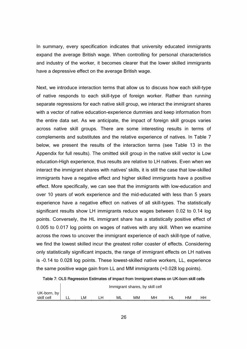
Next, we introduce interaction terms that allow us to discuss how each skill-type

of native responds to each skill-type of foreign worker. Rather than running

separate regressions for each native skill group, we interact the immigrant shares

with a vector of native education-experience dummies and keep information from

the entire data set. As we anticipate, the impact of foreign skill groups varies

across native skill groups. There are some interesting results in terms of

complements and substitutes and the relative experience of natives. In Table 7

below, we present the results of the interaction terms (see Table 13 in the

Appendix for full results). The omitted skill group in the native skill vector is Low

education-High experience, thus results are relative to LH natives. Even when we

interact the immigrant shares with natives' skills, it is still the case that low-skilled

immigrants have a negative effect and higher skilled immigrants have a positive

effect. More specifically, we can see that the immigrants with low-education and

over 10 years of work experience and the mid-educated with less than 5 years

experience have a negative effect on natives of all skill-types. The statistically

significant results show LH immigrants reduce wages between 0.02 to 0.14 log

points. Conversely, the HL immigrant share has a statistically positive effect of

0.005 to 0.017 log points on wages of natives with any skill. When we examine

across the rows to uncover the immigrant experience of each skill-type of native,

we find the lowest skilled incur the greatest roller coaster of effects. Considering

only statistically significant impacts, the range of immigrant effects on LH natives

is -0.14 to 0.028 log points. These lowest-skilled native workers, LL, experience

the same positive wage gain from LL and MM immigrants (+0.028 log points).

Table 7: OLS Regression Estimates of impact from Immigrant shares on UK-born skill cells

Immigrant shares, by skill cell

UK-born, byskill cell LL LM LH ML MM MH HL HM HH

27

LL 0.028* -0.049 -0.14** -0.013 0.028** -0.039** 0.015** 0.015** 0.006

(2.55) (-1.48) (-4.18) (-1.81) (4.29) (-3.65) (2.94) (3.40) (1.03)

LM 0.014* -0.007 -0.048** -0.011** 0.006 -0.008 0.009** 0.005 0.006

(2.43) (-0.42) (-2.94) (-2.87) (1.65) (-1.54) (3.66) (1.95) (1.78)

LH (omitted)

ML 0.021 -0.064 -0.135** -0.008 0.023** -0.021 0.017** 0.015** 0.005

(1.84) (-1.85) (-3.59) (-1.09) (3.42) (-1.79) (3.17) (3.11) (0.81)

MM 0.00 -0.025 -0.02 0.001 0.005 0.005 0.008* 0.002 0.002

(0.00) (-1.08) (-0.87) (0.16) (1.06) (0.71) (2.22) (0.51) (0.54)

MH 0.007 -0.036* -0.052** -0.006 0.004 0.003 0.011** 0.003 0.01**

(1.38) (-2.37) (-2.98) (-1.92) (1.41) (0.52) (4.45) (1.21) (3.30)

HL 0.004 -0.033 -0.061* -0.004 0.012* -0.006 0.011** 0.004 0.007

(0.53) (-1.33) (-2.16) (-0.71) (2.49) (-0.65) (2.74) (1.25) (1.41)

HM 0.004 0.004 -0.03 -0.002 0.002 0.007 0.005 0.003 0.006

(0.61) (0.20) (-1.43) (-0.59) (0.62) (1.08) (1.67) (1.29) (1.54)

HH -0.003 -0.037* -0.059** -0.006 0.006 0.008 0.013** 0.005* 0.005

(-0.59) (-2.30) (-3.17) (-1.82) (1.82) (1.32) (4.96) (2.05) (1.54)

t-stat reported in parenthesis. **- significant at 1%, *- significant at 5%Source: Author's LFS sample, 1993-2005. Employed males only.

In summary, we are able to specify the groups that exert positive and negative

forces on native wages. Unlike previous works, we do not find all groups of

immigrants have a negative impact on low-skilled natives. For the lowest skilled

natives, it appears that the lowest immigrants complement, the mid-skilled

immigrants compete, and the higher skilled immigrants improve productivity. In

addition, there are low-skilled groups of immigrants that have negative effects on

high-skilled natives, which indicates that natives would prefer a larger ratio of

natives with low skills. Although the labour market reacts to supply shocks with

wage and employment impacts, our estimates only determine the price effects

and any workers that leave employment do not influence parameter estimates.

Therefore, there may be larger effects that we are unable to capture.

7.a.2 Effect of immigration on NonUK-born workers

We perform OLS regressions on various model specifications to observe how the

addition of more controls affects the coefficients on our foreign variables. In order

to account for any assimilation effects bias our estimates, we include foreign

28

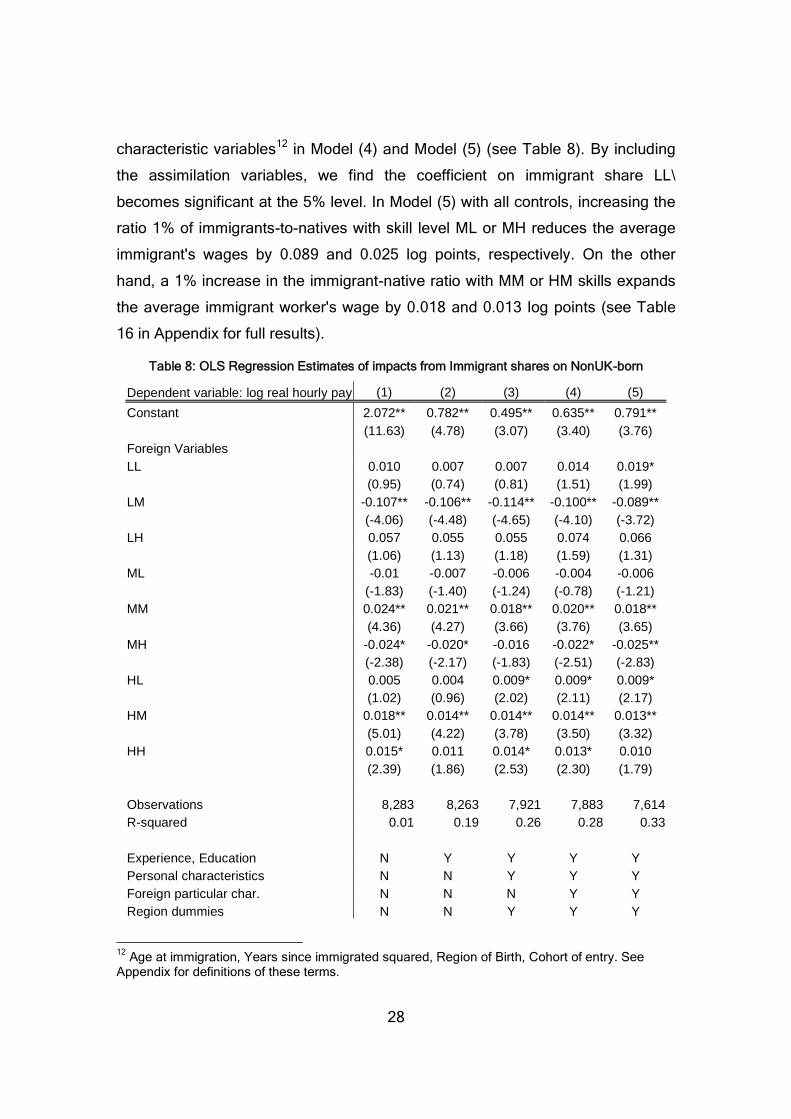
characteristic variables12 in Model (4) and Model (5) (see Table 8). By including

the assimilation variables, we find the coefficient on immigrant share LL\

becomes significant at the 5% level. In Model (5) with all controls, increasing the

ratio 1% of immigrants-to-natives with skill level ML or MH reduces the average

immigrant's wages by 0.089 and 0.025 log points, respectively. On the other

hand, a 1% increase in the immigrant-native ratio with MM or HM skills expands

the average immigrant worker's wage by 0.018 and 0.013 log points (see Table

16 in Appendix for full results).

Table 8: OLS Regression Estimates of impacts from Immigrant shares on NonUK-born

Dependent variable: log real hourly pay (1) (2) (3) (4) (5)

Constant 2.072** 0.782** 0.495** 0.635** 0.791**

(11.63) (4.78) (3.07) (3.40) (3.76)

Foreign Variables

LL 0.010 0.007 0.007 0.014 0.019*

(0.95) (0.74) (0.81) (1.51) (1.99)

LM -0.107** -0.106** -0.114** -0.100** -0.089**

(-4.06) (-4.48) (-4.65) (-4.10) (-3.72)

LH 0.057 0.055 0.055 0.074 0.066

(1.06) (1.13) (1.18) (1.59) (1.31)

ML -0.01 -0.007 -0.006 -0.004 -0.006

(-1.83) (-1.40) (-1.24) (-0.78) (-1.21)

MM 0.024** 0.021** 0.018** 0.020** 0.018**

(4.36) (4.27) (3.66) (3.76) (3.65)

MH -0.024* -0.020* -0.016 -0.022* -0.025**

(-2.38) (-2.17) (-1.83) (-2.51) (-2.83)

HL 0.005 0.004 0.009* 0.009* 0.009*

(1.02) (0.96) (2.02) (2.11) (2.17)

HM 0.018** 0.014** 0.014** 0.014** 0.013**

(5.01) (4.22) (3.78) (3.50) (3.32)

HH 0.015* 0.011 0.014* 0.013* 0.010

(2.39) (1.86) (2.53) (2.30) (1.79)

Observations 8,283 8,263 7,921 7,883 7,614

R-squared 0.01 0.19 0.26 0.28 0.33

Experience, Education N Y Y Y Y

Personal characteristics N N Y Y Y

Foreign particular char. N N N Y Y

Region dummies N N Y Y Y

12Age at immigration, Years since immigrated squared, Region of Birth, Cohort of entry. See

Appendix for definitions of these terms.

29

Industry dummies N N N N Y

t-stat reported in parenthesis. **- significant at 1%, *- significant at 5%Source: Author's LFS sample, 1993-2005. Employed males only.

Comparing immigrant and native responses, the results in Model (5) for

immigrants (see Table 8) and Model (4) for natives (see Table 6) indicate that

immigration to Britain has only a slightly different impact on immigrant and native

workers. Generally, it appears that natives absorb the wage impact more than

immigrants. The ratio of LH immigrants has a -0.089 log point effect on average

immigrant wage and a -0.023 log point on the average native's wages. On the

positive spectrum, the effects are 0.004 and 0.013 log points for natives and

immigrants, respectively.

Between skill group regression analysis reveals there are only a couple of skill

groups that experience a differential impact of immigration (see Table 15 for full

results). The results below (Table 9) indicated upward pressure on wages from

LL immigrant share and we discover here that the statistically significant groups

to receive this benefit are LL, MM, and MH immigrants. It seems rather odd the

LL immigrant share has a more positive impact on LL immigrants than those with

LH skills. However, when we look at the higher-skilled immigrants it once again

appears that there are positive effects associated with similarly skilled immigrant

shares. It is possible that there are network effects between workers with similar

skills and this is stronger for immigrants than natives. This would be an

interesting avenue of research, however it is beyond the scope of this paper to

determine the validity of our suggestion.

Table 9 OLS Regression Estimates of impact from Immigrant shares on NonUK-born skill cells

Immigrant share, by skill

Immigrants,by skill LL LM LH ML MM MH HL HM HH

LL 0.176* 0.284 0.06 -0.028 0.058 0.018 0.018 -0.058 -0.097

(2.04) (1.20) (0.22) (0.53) (1.32) (0.19) (0.48) (-1.79) (-1.81)

LM 0.065 0.102 0.015 0.004 0.010 -0.042 -0.003 -0.014 -0.001

(1.79) (0.96) (0.14) (0.18) (0.47) (-1.19) (-0.17) (-0.90) (-0.06)

LH (omitted)

ML -0.035 -0.119 -0.027 -0.012 -0.017 -0.067 0.062* 0.023 -0.011

30

(-0.59) (-0.60) (-0.12) (-0.28) (-0.47) (-0.87) (1.96) (0.85) (-0.31)

MM 0.066* -0.09 0.115 -0.009 0.023 -0.082** 0.029* -0.011 0.007

(2.31) (-1.07) (1.18) (-0.49) (1.45) (-2.73) (2.02) (-0.92) (0.38)

MH 0.041* -0.011 0.059 0.001 0.001 -0.035 0.006 0.000 -0.001

(2.05) (-0.19) (0.84) (0.05) (0.08) (-1.57) (0.65) (0.05) (-0.04)

HL 0.017 0.019 0.01 -0.007 0.001 0.001 0.002 0.011 -0.016

(0.69) (0.27) (0.12) (-0.49) (0.10) (0.03) (0.18) (1.07) (-1.05)

HM 0.019 -0.066 0.120* 0.002 0.030** -0.052** -0.005 0.013 0.000

(1.12) (-1.42) (2.00) (0.18) (3.14) (-2.81) (-0.59) (1.91) (0.03)

HH 0.011 -0.129** 0.02 0.005 0.02* -0.022 0.007 0.007 0.018

(0.69) (-2.76) (0.33) (0.48) (2.15) (-1.16) (0.83) (1.00) (1.68)

t-stat reported in parenthesis. **- significant at 1%, *- significant at 5%Source: Author's LFS sample, 1993-2005. Employed males only.

Between group effects also show that immigrants face statistically significant

impacts from only one or two immigrant skill groups. For example, immigrants

with LL skills incur a 0.176 log point increase by increasing the ratio of

immigrants-to-natives with the LL skills by 1 log percentage point. All models of

the initial regressions (see Table 8) indicate downward pressure on wages due to

the share of MH immigrants. Through the following regression analysis, we can

be more explicit and specify a great deal of the disadvantage, -0.082 and -0.052

log points, is on immigrants with skill set MM and HM.

The range of techniques and specifications we implement provides a more

complete picture of immigrants in the British workforce. Results indicate that the

OLS estimates are fairly accurate across the earnings distribution for most

immigrant skill groups. Nevertheless, we do find some differences in the LM

immigrant share where coefficients decrease further across the quantiles. This

indicates with a larger share of LH immigrants, individuals in the upper 10 percent

of UK earnings have lower earnings than would be expected. Another way of

stating this is that individuals in a labour market with higher ratios of LH

immigrants whom are in the bottom quantile of earnings, their earnings difference

is compressed relative to those in the median group. In addition, the HH

immigrant share has a more positive effect across the earnings distribution.

Comparing this with OLS results, we see that HH immigrant share increases

average earnings. Therefore, we can interpret QR results to mean that a larger

share of HH immigrants expands earnings for individuals with greater ability.

31

7.b Quantile Results, A Robustness Check

7.b.1 Effect of immigration on UK-born workers

Quantile regression estimates demonstrate the effect of immigrants on natives'

wages depends on the ability of natives. In order to compare OLS and QR

results, Table 10 presents quantile estimates and the previously determined OLS

estimates (see Table 13 in Appendix B for full quantile regression results). The

most striking result is to find OLS results hide the impact of LH immigrants on

low-ability natives. In OLS estimates, the LH ratio is statistically insignificant;

however, QR estimates show that this group has a negative impact (-0.034 log

points) on the conditional wages of low-ability natives. Coefficients on LH

become increasingly positive, yet statistically insignificant, across the quantiles.

Therefore, LH immigrants have a smaller impact on earnings at the upper

quantiles of the earnings distribution. This indicates that the share of LH

immigrants have no effect on average wages, yet individuals in the bottom 10

percent of UK earnings have lower earnings than would be expected for a larger

ratio of immigrants with LH skills.

Table 10: OLS & QR Regression Estimates of impact from Immigrant shares on UK-born skillcells

OLS Quantiles

UK-born, by skillshare 0.10 0.25 0.50 0.75 0.90

LL 0.006** 0.009** 0.004* 0.004* 0.001 0.00

(2.71) (3.65) (2.26) (2.39) (0.42) (0.10)

LM -0.023** -0.008 -0.022** -0.016** -0.024** -0.014

(3.92) (-1.11) (-3.52) (-3.41) (-3.83) (-1.63)

LH -0.010 -0.034* -0.01 0.001 0.014 0.007

(-0.88) (-2.55) (-0.76) (0.10) (1.24) (0.34)

ML -0.003* -0.004* -0.004* -0.003* -0.001 -0.002

(-2.36) (-2.07) (-2.41) (-2.17) (-0.56) (-0.82)

MM 0.005** 0.006** 0.004** 0.003* 0.005** 0.005*

(4.51) (2.65) (2.75) (2.46) (3.71) (2.57)

MH -0.001 -0.002 0.001 0.002 -0.001 0.003

(-0.28) (-0.69) (0.65) (1.14) (-0.24) (0.91)

HL 0.010** 0.01** 0.01** 0.009** 0.007** 0.008**

(9.73) (6.69) (10.46) (8.58) (6.58) (4.23)

HM 0.004** 0.002 0.004** 0.003** 0.005** 0.003**

(4.55) (1.45) (5.57) (5.09) (5.38) (2.68)

32

HH 0.005** 0.002 0.005** 0.005** 0.006** 0.005**

(4.01) (1.47) (3.71) (5.47) (4.75) (3.30)

Observations 120,650 120,650

Pseudo R-squared 0.33 0.181 0.207 0.221 0.219 0.207

t-stat reported in parenthesis. **- significant at 1%, *- significant at 5%Source: Author's LFS sample, 1993-2005. Employed males only.

7.b.2 Effect of immigration on NonUK-born workers

In a final calculation of the immigrant effect, we perform a quantile regression on

Model (5)13 and investigate the impact of immigration on immigrants across the

wage distribution. Coefficients on the foreign variables are displayed in Table 11

(for full results, see Table 17 in the Appendix). Results show the OLS estimates

do not capture the entire story regarding immigrant impacts on other immigrants.

Beginning with the immigrant share of LL workers, OLS estimates report 0.204

log point increase in average wages. Quantile estimates indicate conditional

wages of higher skilled workers, those in the top 25% of conditional wages (or in

the .75 and .90 quantiles), reduce the positive effect of LL immigrants; coefficient

estimates are 0.191 for the 75th percentile and 0.065 for the 90th percentile as

opposed to 0.272 for the 10th percentile. Increasing the ratio of LH immigrants-to-

natives has a less negative effect on the highest ability immigrants. More

importantly, quantile regression estimates illustrate how the OLS technique

misrepresents the downward pressure of LH immigrants on wages. OLS

estimates indicate a wage reduction of -0.116 log points with a 1% increase in the

ratio of LH immigrants-to-natives, whilst QR results show that the effect of this

ratio is greater at the 10th (-0.177) and 50th (-0.175) percentiles. We do find,

however, the OLS technique accurately estimates the effect of ML immigrants,

such that the QR estimates are similar across the quantiles.

Table 8: OLS & QR Regression Estimates of impact from Immigrant shares on NonUK-born skillcells

OLS Quantiles

Immigrant share,by skill 0.10 0.25 0.50 0.75 0.90

LL 0.019* 0.015 0.021 0.017 0.018 0.007

13From Table 8

33

(1.99) (0.79) (1.44) (1.68) (1.51) (0.42)

LM -0.089** -0.067* -0.084* -0.102** -0.106** -0.125*

(-3.72) (-1.97) (-2.70) (-4.43) (-2.94) (-2.36)

LH 0.066 0.114 0.044 0.098* 0.074 -0.009

(1.31) (1.47) (0.73) (2.21) (1.16) (-0.09)

ML -0.006 0.003 0.001 -0.002 -0.013 -0.022

(-1.21) (0.28) (0.07) (-0.52) (-1.95) (-1.90)

MM 0.018** 0.014 0.012 0.018** 0.018** 0.017*

(3.65) (1.76) (1.92) (3.57) (3.15) (2.23)

MH -0.025** -0.03* -0.019* -0.016 -0.027* -0.012

(-2.83) (-2.43) (-2.17) (-1.22) (-2.52) (-0.71)

HL 0.009* 0.003 0.011* 0.007 0.015** 0.02**

(2.17) (0.42) (2.01) (1.48) (2.93) (2.73)

HM 0.013** 0.011* 0.008* 0.014** 0.014* 0.021**

(3.32) (2.22) (1.98) (3.36) (2.51) (3.16)

HH 0.010 0.003 0.005 0.009 0.019* 0.023*

(1.79) (0.35) (0.58) (1.47) (2.37) (2.03)

Observations 7,614 7,614

Pseudo R-squared 0.33 0.155 0.197 0.221 0.221 0.228

t-stat reported in parenthesis. **- significant at 1%, *- significant at 5%

Source: Author's LFS sample, 1993-2005. Employed males only.

Quantile regression results indicate the OLS estimates are accurate. Excluding a

few skill groups, the OLS and QR are very similar and suggest there is no

unobserved heterogeneity affecting results. In other words, the ability to absorb

immigrant workers is largely from matching skill needs in terms of education-

experience. Native and immigrant unobserved ability to interact with immigrants

is not the force behind wage impacts of immigrants in the workforce.

8. Conclusion

In March 2007, former Federal Reserve Chairman Alan Greenspan suggested

the United States reduce wage inequality by encouraging in-migration of high-

skilled workers.14 The theory is there will be relatively more high-skilled workers

competing for fewer jobs and wages will fall relative to low-skilled workers. This is

a rather simplistic interpretation of the labour market and does not take into

14http://www.bloomberg.com/apps/news?pid=newsarchive\&sid=aDWi3n1erxT8. Accessed on

28/03/07.

34

account nuances of worker relationships. The numbers of high-skilled immigrants

it would take to begin pushing down wages of the most educated and

experienced individuals is beyond any amount the public and its government

would allow. High-skilled workers are able to take advantage of the opportunities

brought about by immigrant workers and expand earnings potential. Lower-skilled

workers take the available, low paying jobs.

This paper does not support the broad hypothesis that high-skilled immigrants

will drive down high-skilled wages. In fact, highly educated NonUK-born workers

with limited experience push up the wages of all native workers. There is a great

deal of complementarity between high-skilled, low-experience foreign workers

and other skill types of workers. It appears they are a very adaptable group of

workers and positively influence the productivity of natives across the earnings

distribution. Policies encouraging the in-migration of these workers do not reduce

wage inequality, but do improve wages for all workers.

In contrast, highly educated immigrants with more than five years work

experience increase wages for all but the lowest ability native workers. This has

the consequence of increasing wage inequality. However, it is important to

reiterate that this is only one way to interpret results. It is highly probable that the

influx of immigrants with high education and experience increase trade and

growth, which can positively yet indirectly affect low wage earners. What we

calculate here is the direct effect on an individual's marginal productivity.

We find immigrants with similar skill set to natives improve the wages of their

counterparts. We offer a couple of explanations for this. Firstly, there are network

effects in force where people communicate with other workers of similar skill

levels, exchange information, and push up wages. This may be why we find

positive effects between same skill cells are stronger for immigrants. Another

possibility is this finding is the result of positive competition between workers,

which improves productivity or wages. Lastly, we must consider these positive

findings may be attributed to uncontrolled selectivity.

35

9. References

Angrist, J. and A. Krueger (1999). Emprical Strategies in Labor Markets. In O.

Ashenfelter and D. Card (eds), The Handbook of Labor Economics, Vol. 3,

North Holland.

Becker, Gary (1975). Human Capital. National Bureau of Economic Research,

New York.

Blanchflower, David G., Jumana Saleheen, and Chris Shadforth (2007). "The

Impact of the Recent Migration from Eastern Europe on the UK Economy",

Institute for the Study of Labor, Discussion Paper No 2615.

Borjas, George, Richard Freeman, and Lawrence Katz (1996). "Searching for the

Effect of Immigration on the Labor Market", American Economic Review,

86(2), Papers and Proceedings of the Hundredth and Eight Annual

Meeting of the American Economic Association San Francisco, pp.246-

251.

Borjas, G. (1997). "To Ghetto or Not to Ghetto: Ethnicity and Residential

Segregation", NBER Working Papers 6176, National Bureau of Economic

Research.

Borjas, George (2003). "The Labour Demand Curve is Downward Sloping:

Reexamining the Impact of Immigration on the Labor Market", The

Quarterly Journal of Economics, pp. 1335-1374.

Buchinsky, Moshe (1998). "Recent Advances in Quantile Regression Models: A

Practical Guideline for Empirical Research", The Journal of Human

Resources, 33(1), pp. 88-126.

Card, David (1999). "The Impact of the Mariel Boatlift on the Miami Labor

Market", Industrial and Labor Relations Review, 43(2), pp. 245-257.

Card, D. and J. Dinardo (2000). "Do Immigrant Inflows Lead to Native Outflows?",

American Economic Review, 90(2), Papers and Proceedings of the One

Hundred Twelfth Annual Meeting of the American Economic Association,

pp. 360-67.

Card, David and Thomas Lemieux (2001). "Can Falling Supply Explain the Rising

Return to College for Younger Men? A Cohort-Based Analysis.", The

36

Quarterly Journal of Economics, 116, pp. 705-46.

Dustmann, Christian, Francesca Fabbri, and Ian Preston (2005). "The Impact of

Immigration of the British Labour Market." The Economic Journal, 115, pp.

F324-F41.

Filer, R. (1992). The Effect of Immigrant Arrivals on Migratory Patterns of Native

Workers. In Borjas, G. and R. Freeman (eds.), Immigration and the Work

Force. Chicago: University of Chicago Press, pp. 245-69.

Frey, W. (1995). "Immigration and internal migration `flight' from the US

metropolitan areas: Toward a new demographic balkanisation", Urban

Studies, 4-5, pp. 733-57.

Friedberg, Rachel M. (2001). "The Impact of Mass Migration on the Israeli Labor

Market", Quarterly Journal of Economics, 116(4), pp. 1373-408.

Gaston, Noel and Douglas Nelson (2001). "The Employment and Wage Effects of

Immigration: Trade and Labour Economics Perspectives", University of

Nottingham, Globalisation and Labour Markets Programme, Research

Paper 2001/28.

Hatton, Timothy J. and Massimiliano Tani (2005). "Immigration and Inter-

Regional Mobility in the UK, 1982-2000", The Economic Journal , 115, pp.

F342-F358.

Heckman, Lochner, and Todd (2005). "Earnings Functions, Rates of Return and

Treatment Effects: The Mincer Equation and Beyond", Institute for the

Study of Labor, Discussion Paper No. 1700.

Koenker, Roger and Gilbert Bassett (1978). "Regression Quantiles",

Econometrica, 46(1), pp. 33-50.

Machado, Jose and Jose Mata (2005) . "Counterfactual Decomposition of

Changes in Wage Distributions Using Quantile Regression", Journal of

Applied Econometrics, 20, pp. 445-65.

Manacorda, Marco, Alan Manning, and Jonathan Wadsworth (2006). "The Impact

of Immigration on the Structure of Male Wages: Theory and Evidence from

Britain", CReAM, Discussion Paper No 08/06.

Mincer, Jacob (1974). "Schooling, Experience and Earnings", National Bureau of

Economic Research. New York.

37

Ottaviano, Gianmarco I.P. and Giovanni Peri (2006). "Rethinking the Gains from

Immigration: Theory and Evidence from the U.S", NBER Discussion Paper

11672.

Portes, Jonathan and Simon French (2005). "The impact of free movement of

workers from central and eastern Europe on the UK labour market: early

evidence", Department for Work and Pensions, Working Paper No 18.

Tannuri-Pianto, Maria (2002). "Relative Earnings of Immigrants and Natives

under Changes in the US Wage Structure, 1970-1990: A Quantile

Regression Approach", Department of Economics, University of Brasilia,

Working Paper 264.

10. Appendix A (Variable Definitions)

Dependent Variable

Log Real Hourly Wage- the LFS does not ask income questions to the self-

employed. LFS asks all persons 16-69, and those over 70 whom are employed.

`Gross weekly pay in main job' (GRSSWK) is asked each quarter, but only to

individuals in their 5th wave. From 1997 onwards, the question was asked in the

1st wave as well. We checked for any significant disparities or changes from the

1st to 5th wave, there were none. If GRSSWK is greater than £3,500, or

GRSSWK is greater than £1,000 and the respondent is a manual worker, then

the LFS does not give an income weight. Non-response to this question is also

be zero-weighted. LFS Users Guide indicates that standard filters used to

calculate average gross weekly earnings are GRSSWK>0. To generate hourly

pay, we also filter on `usual hours excluding overtime', USUHR>0. To produce

real wages, we use the U.K Retail Price Index to inflate wages based on 2005Q4

prices. We then generate logarithm of the gross real hourly wage.

Personal and Productivity Variables

Education- is equal to leaving age minus 5 (to account for the age of starting

school).

Experience- is potential labour market experience in that it is derived from the

respondents' age minus leaving age from education (EDAGE) for individuals who

38

responded to EDAGE. If an individual answered (s)he `never had any education',

we use age minus 15. This is because there is a legal working age and legal

leaving age from education.

Full-time- we create a dummy equal to 1 if the response to USUHR is greater

than 30. It is equal to 0 if the response is 30 hours or less.

Industry- this is only reported by respondents in employment and not tied to

company sponsored college. There are ten categories: (1) Agriculture and

fishing, (2) Energy and water, (3) Manufacturing, (4) Construction, (5)

Distribution, hotels, and restaurants, (6) Transport and communication, (7)

Banking, finance, and insurance, (8) Public administration, education, and health,

(9) Other services.

Married- we use the variable `marital status', MARSTT, and 'living together as a

couple', LIVTOG. We move all the responses of `does not apply' or `no answer' to

missing. Our variable takes a value of 1 if the response is `married, living with

husband or wife' or a yes response to LIVTOG, zero otherwise.

Nonwhite- there are several ethnicity variables over time, ETH01, ETHCEN15,

ETHCEN6, which are recoded for consistency: (1) White, (2) Mixed, (3) Asian or

Asian British, (4) Black or Black British, (5) Chinese, (6) Other. We then give a

value of 0 to responses of white and 1 otherwise.

Region- we create dummies to the response of `region of usual residence',

URESMC. We create one response of inner and outer London, as well as

Strathclyde \ and Rest of Scotland. We drop Northern Ireland.

Immigrant ratio {LL-HH}- the vector of education groups is derived from `leaving

age from education', EDAGE. The groups are: (Low) ≤16 leaving age, (Mid) 17-

18, (High) 19+. The vector of experience groups is created by potential

experience of age minus education leaving age: (Low) ≤5 years, (Mid) 6-15,

(High) 16+. These dummies are interacted to create the nine skill groups. The

number of immigrants in each skill cell is divided into the number of natives in the

same skill cell per year.

11. Appendix B

11.a. Figures

39

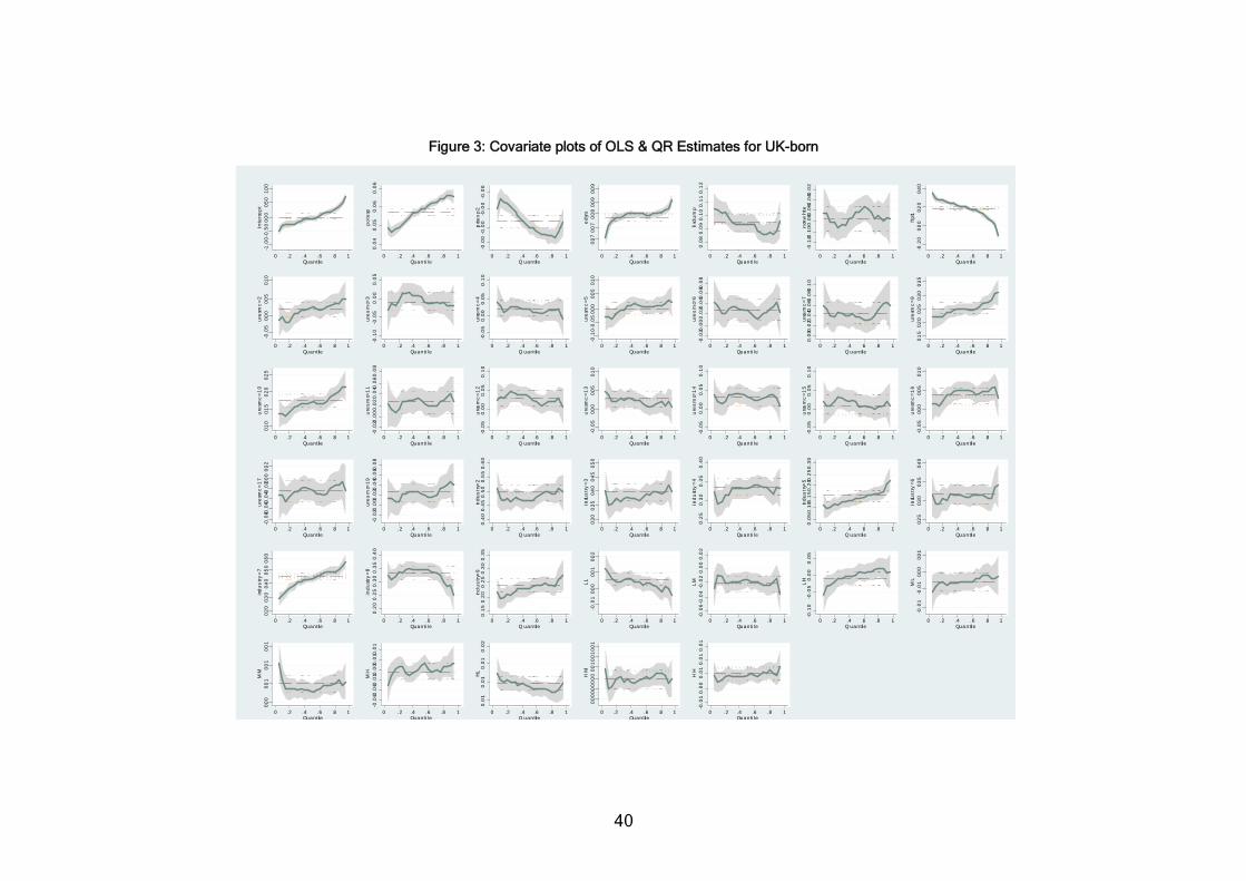
40

Figure 3: Covariate plots of OLS & QR Estimates for UK-born

-1.0

0-0

.50

0.0

00

.50

1.0

0

Inte

rce

pt

0 .2 .4 .6 .8 1Quantil e

0.0

40

.05

0.0

60

.06

po

texp

0 .2 .4 .6 .8 1Quanti l e

-0.0

0-0

.00

-0.0

0-0

.00

pot

ex

p2

0 .2 .4 .6 .8 1Q uantil e

0.0

70

.07

0.0

80

.09

0.0

9

ed

yrs

0 .2 .4 .6 .8 1Quantil e

0.0

80

.09

0.1

00

.11

0.1

2

livd

um

p

0 .2 .4 .6 .8 1Quanti le

-0.1

2-0.1

0-0

.08-0

.06-0

.04-0

.02

non

wh

ite

0 .2 .4 .6 .8 1Q uantile

-0.2

00

.00

0.2

00

.40

ftp

t1

0 .2 .4 .6 .8 1Qua ntil e

-0.0

50

.00

0.0

50

.10

ure

smc

=2

0 .2 .4 .6 .8 1Quantil e

-0.1

0-0

.05

0.0

00

.05

ure

sm

c=3

0 .2 .4 .6 .8 1Quanti l e

-0.0

50

.00

0.0

50

.10

ure

sm

c=

4

0 .2 .4 .6 .8 1Q uantil e

-0.1

0-0

.05

0.0

00

.05

0.1

0

ure

smc

=5

0 .2 .4 .6 .8 1Quantil e

-0.0

20.0

00

.020

.040

.060

.08

ure

sm

c=6

0 .2 .4 .6 .8 1Quanti le

0.0

00.0

20.0

40.0

60.0

80.1

0u

res

mc

=7

0 .2 .4 .6 .8 1Q uantile

0.1

50

.20

0.2

50

.30

0.3

5

ure

smc

=9

0 .2 .4 .6 .8 1Qua ntil e

0.1

00

.15

0.2

00

.25

ure

smc

=1

0

0 .2 .4 .6 .8 1Quantil e

-0.0

20.0

00

.02

0.0

40.0

60

.08

ure

sm

c=1

1

0 .2 .4 .6 .8 1Quanti l e

-0.0

50

.00

0.0

50

.10

ure

sm

c=

12

0 .2 .4 .6 .8 1Q uantil e

-0.0

50

.00

0.0

50

.10

ure

smc

=1

3

0 .2 .4 .6 .8 1Quantil e

-0.0

50

.00

0.0

50

.10

ure

sm

c=1

4

0 .2 .4 .6 .8 1Quanti le

-0.0

50

.00

0.0

50

.10

ure

sm

c=

15

0 .2 .4 .6 .8 1Q uantile

-0.0

50

.00

0.0

50

.10

ure

smc

=1

6

0 .2 .4 .6 .8 1Qua ntil e

-0.0

8-0.0

6-0.0

4-0.0

20.0

00

.02

ure

smc

=1

7

0 .2 .4 .6 .8 1Quantil e

-0.0

20.0

00.0

20.0

40.0

60.0

8

ure

sm

c=1

9

0 .2 .4 .6 .8 1Quanti l e

0.4

00

.45

0.5

00

.55

0.6

0in

du

str

y=2

0 .2 .4 .6 .8 1Q uantil e

0.3

00

.35

0.4

00

.45

0.5

0

indu

str

y=

3

0 .2 .4 .6 .8 1Quantil e

0.2

50

.30

0.3

50

.40

ind

ust

ry=

4

0 .2 .4 .6 .8 1Quanti le

0.0

50

.100

.15

0.2

00.2

50

.30

ind

us

try=

5

0 .2 .4 .6 .8 1Q uantile

0.2

50

.30

0.3

50

.40

indu

str

y=

6

0 .2 .4 .6 .8 1Qua ntil e

0.2

00

.30

0.4

00

.50

0.6

0

ind

us

try

=7

0 .2 .4 .6 .8 1Quantil e

0.2

00

.25

0.3

00

.35

0.4

0

ind

ust

ry=

8

0 .2 .4 .6 .8 1Quanti l e

0.1

50

.20

0.2

50

.30

0.3

5in

du

str

y=9

0 .2 .4 .6 .8 1Q uantil e

-0.0

10

.00

0.0

10

.02

LL

0 .2 .4 .6 .8 1Quantil e

-0.0

6-0

.04

-0.0

20

.00

0.0

2

LM

0 .2 .4 .6 .8 1Quanti le

-0.1

0-0

.05

0.0

00

.05

LH

0 .2 .4 .6 .8 1Q uantile

-0.0

1-0

.01

0.0

00

.01

ML

0 .2 .4 .6 .8 1Qua ntil e

0.0

00

.01

0.0

10

.01

MM

0 .2 .4 .6 .8 1Quantil e

-0.0

1-0.0

1-0.0

10.0

00.0

10.0

1

MH

0 .2 .4 .6 .8 1Quanti l e

0.0

10

.01

0.0

10

.02

HL

0 .2 .4 .6 .8 1Q uantil e

0.0

00

.00

0.0

00

.01

0.0

10

.01

HM

0 .2 .4 .6 .8 1Quantil e

-0.0

10

.00

0.0

10

.01

0.0

1

HH

0 .2 .4 .6 .8 1Quanti le

41

Figure 4: Covariate plots of OLS & QR Estimates for NonUK-born

-1.0

00.0

01.0

02

.003

.00

Inte

rcep

t

0 .2 .4 .6 .8 1Quanti l e

0.0

00

.020

.04

0.0

60

.08

pot

exp

0 .2 .4 .6 .8 1Qua ntile

-0.0

0-0.0

0-0.0

0-0.0

0-0.0

0-0.0

0

po

texp

2

0 .2 .4 .6 .8 1Q uanti le

0.0

30.0

40.0

50.0

60.0

70.0

8ed

yrs

0 .2 .4 .6 .8 1Quanti l e

-0.0

50.0

00.0

50

.10

0.1

5liv

dum

p

0 .2 .4 .6 .8 1Quantil e

-0.2

5-0.2

0-0

.15-0

.10

-0.0

5

no

nwh

ite

0 .2 .4 .6 .8 1Q uanti le

0.0

00.1

00.2

00.3

00.4

00.5

0ftp

t1

0 .2 .4 .6 .8 1Quanti le

-0.0

2-0.0

10.0

00.0

10.0

20.0

3ag

eat

imm

0 .2 .4 .6 .8 1Quantil e

-0.0

00.0

00

.00

0.0

00.0

0yr

ssin

ces

q

0 .2 .4 .6 .8 1Quanti l e

-0.2

0-0.1

00.0

00.1

00.2

0re

gob=

2

0 .2 .4 .6 .8 1Qua ntile

-0.4

0-0

.200

.00

0.2

0

rego

b=3

0 .2 .4 .6 .8 1Q uanti le

-0.2

0-0.1

5-0.1

0-0.0

50.0

0re

gob

=4

0 .2 .4 .6 .8 1Quanti l e

-0.3

0-0.2

0-0.1

00.0

00.1

00.2

0re

gob=

5

0 .2 .4 .6 .8 1Quantil e

-0.4

0-0

.20

0.00

0.20

rego

b=6

0 .2 .4 .6 .8 1Q uanti le

-0.1

00.

00

0.1

00.

20

reg

ob=7

0 .2 .4 .6 .8 1Quanti le

-0.3

0-0.2

0-0

.100

.000

.10

rego

b=8

0 .2 .4 .6 .8 1Quantil e

-0.2

00

.00

0.2

00

.40

cohg

rp=

2

0 .2 .4 .6 .8 1Quanti l e

-0.2

0-0.1

00.0

00.1

00.2

00.3

0c

ohgr

p=3

0 .2 .4 .6 .8 1Qua ntile

-0.4

0-0.

200.

00

0.2

00.

40

coh

grp

=4

0 .2 .4 .6 .8 1Q uanti le

-0.4

0-0.

200.0

00.2

00.

40

cohg

rp=

5

0 .2 .4 .6 .8 1Quanti l e

-0.6

0-0.4

0-0.2

00.0

00.2

00.4

0co

hgr

p=6

0 .2 .4 .6 .8 1Quantil e

-0.6

0-0.4

0-0.2

00.00

0.20

0.40

coh

grp

=7

0 .2 .4 .6 .8 1Q uanti le

-1.0

0-0

.50

0.0

00.

50

coh

grp

=8

0 .2 .4 .6 .8 1Quanti le

-1.0

0-0

.50

0.0

00

.50

coh

grp

=9

0 .2 .4 .6 .8 1Quantil e

-1.0

0-0.5

00.0

00

.501

.00

cohg

rp=

10

0 .2 .4 .6 .8 1Quanti l e

-1.0

0-0

.50

0.0

00

.50

coh

grp

=11

0 .2 .4 .6 .8 1Qua ntile

-0.2

00.0

00.2

00.4

00.6

0

ure

sm

c=2

0 .2 .4 .6 .8 1Q uanti le

-0.4

0-0.2

00.0

00.2

00.4

0ur

esm

c=

3

0 .2 .4 .6 .8 1Quanti l e

-0.4

0-0.2

00.0

00

.200

.40

ures

mc=

4

0 .2 .4 .6 .8 1Quantil e

-0.4

0-0.2

00.

000.

200.

40

ure

sm

c=5

0 .2 .4 .6 .8 1Q uanti le

-0.4

0-0.2

00.0

00.2

00.

40

ure

smc

=6

0 .2 .4 .6 .8 1Quanti le

-0.2

00

.00

0.2

00

.40

ures

mc=

7

0 .2 .4 .6 .8 1Quantil e

-0.2

00.0

00

.200

.40

0.6

0ur

esm

c=

9

0 .2 .4 .6 .8 1Quanti l e

-0.2

00

.00

0.2

00.4

00

.60

ure

sm

c=1

0

0 .2 .4 .6 .8 1Qua ntile

-0.2

00.

00

0.2

00.

40

ure

sm

c=1

1

0 .2 .4 .6 .8 1Q uanti le

-0.4

0-0.

200.

000

.200

.40

ure

smc

=12

0 .2 .4 .6 .8 1Quanti l e

-0.2

00.0

00.2

00.4

00

.60

ures

mc=

13

0 .2 .4 .6 .8 1Quantil e

-0.4

0-0

.20

0.00

0.20

0.40

ure

sm

c=1

4

0 .2 .4 .6 .8 1Q uanti le

-0.5

00.

00

0.5

0ur

esm

c=1

5

0 .2 .4 .6 .8 1Quanti le

-0.2

00

.00

0.2

00

.40

ures

mc=

16

0 .2 .4 .6 .8 1Quantil e

-0.2

00.0

00.2

00

.400

.60

ure

smc

=17

0 .2 .4 .6 .8 1Quanti l e

-0.2

00.0

00.2

00.4

00.6

0u

res

mc=

19

0 .2 .4 .6 .8 1Qua ntile

-0.5

00.0

00.

50

1.0

0

indu

stry

=2

0 .2 .4 .6 .8 1Q uanti le

-1.0

0-0.

500.

00

0.5

01.0

0in

dus

try=3

0 .2 .4 .6 .8 1Quanti l e

-0.5

00

.00

0.5

01

.00

ind

ustry

=4

0 .2 .4 .6 .8 1Quantil e

-1.0

0-0

.50

0.00

0.50

indu

stry

=5

0 .2 .4 .6 .8 1Q uanti le

-1.0

0-0

.500.

00

0.5

01.0

0in

dust

ry=

6

0 .2 .4 .6 .8 1Quanti le

-0.5

00

.00

0.5

01

.00

ind

ustr

y=7

0 .2 .4 .6 .8 1Quantil e

-1.0

0-0.5

00.0

00.5

01

.00

indu

stry

=8

0 .2 .4 .6 .8 1Quanti l e

-0.5

00

.00

0.5

01

.00

indu

stry

=9

0 .2 .4 .6 .8 1Qua ntile

-0.0

4-0.0

20.0

00.0

20.0

40.0

6

LL

0 .2 .4 .6 .8 1Q uanti le

-0.2

0-0

.10

0.0

00.

10

LM

0 .2 .4 .6 .8 1Quanti l e

-0.4

0-0.2

00.0

00.2

00

.40

LH

0 .2 .4 .6 .8 1Quantil e

-0.0

6-0.0

4-0.0

20.0

00.

02

ML

0 .2 .4 .6 .8 1Q uanti le

-0.0

20.0

00.

020

.04

0.0

6M

M

0 .2 .4 .6 .8 1Quanti le

-0.0

8-0.0

6-0.0

4-0.0

20.0

00.0

2M

H

0 .2 .4 .6 .8 1Quantil e

-0.0

20

.00

0.0

20

.04

HL

0 .2 .4 .6 .8 1Quanti l e

-0.0

10.0

00.0

10.0

20.0

30.0

4H

M

0 .2 .4 .6 .8 1Qua ntile

-0.0

20.

00

0.0

20.

04

HH

0 .2 .4 .6 .8 1Q uanti le

42

11.a. Tables

Table 9: OLS Regression Estimates of Immigrant impacts on UK-born wages

Dependent variable: Log real hourly wage Coefficients

Constant 0.591**

(13.98)

Potential Experience 0.054**

(123.15)

Potential Experience Sqrd/1000 -0.001**

(-104.53)

Years of Education 0.079**

(136.17)

Married & cohab 0.095**

(31.27)

Nonwhite -0.074*

(-6.31)

Full-time 0.185**

(20.86)

Region of Residence

Rest of South East (omitted)

Tyne & Wear -0.175**

(-18.25)

Rest of Northern Region -0.158**

(-21.66)

South Yorkshire -0.182**

(-20.36)

West Yorkshire -0.154**

(-21.83)

Rest of Yorkshire & Humberside -0.175**

(-22.08)

East Midlands -0.145**

(-26.72)

East Anglia -0.13**

(-18.55)

Inner & Outer London 0.079**

(14.52)

South West -0.149**

(-28.99)

West Midlands (Metro) -0.145**

(-20.80)

Rest of West Midlands -0.149**

(-24.08)

Greater Manchester -0.141**

(-20.08)

Merseyside -0.163**

(-16.27)

43

Rest of North West -0.14**

(-20.34)

Wales -0.20**

(-30.12)

Industries

Manufacturing (omitted)

Strathclyde & Rest of Scotland -0.149**

(-30.30)

Agriculture & Fishing -0.397**

(-23.53)

Energy & Water 0.097**

(6.67)

Construction -0.06**

(-4.87)

Distribution, Hotels & Restaurants -0.243**

(-19.26)

Transport & Communication -0.08**

(-6.23)

Banking, Finance & Insurance etc 0.054**

(4.31)

Public admin, Educ & Health -0.066**

(-5.25)

Other Services -0.157**

(-12.41)

Foreign Variables

LL 0.006**

(2.71)

LM -0.023**

(-3.92)

LH -0.01

(-0.88)

ML -0.003*

(-2.36)

MM 0.005**

(4.51)

MH -0.001

(-0.28)

HL 0.01**

(9.73)

HM 0.004**

(4.55)

HH 0.005**

(4.01)

Observations 120,650

Pseudo R-squared 0.33

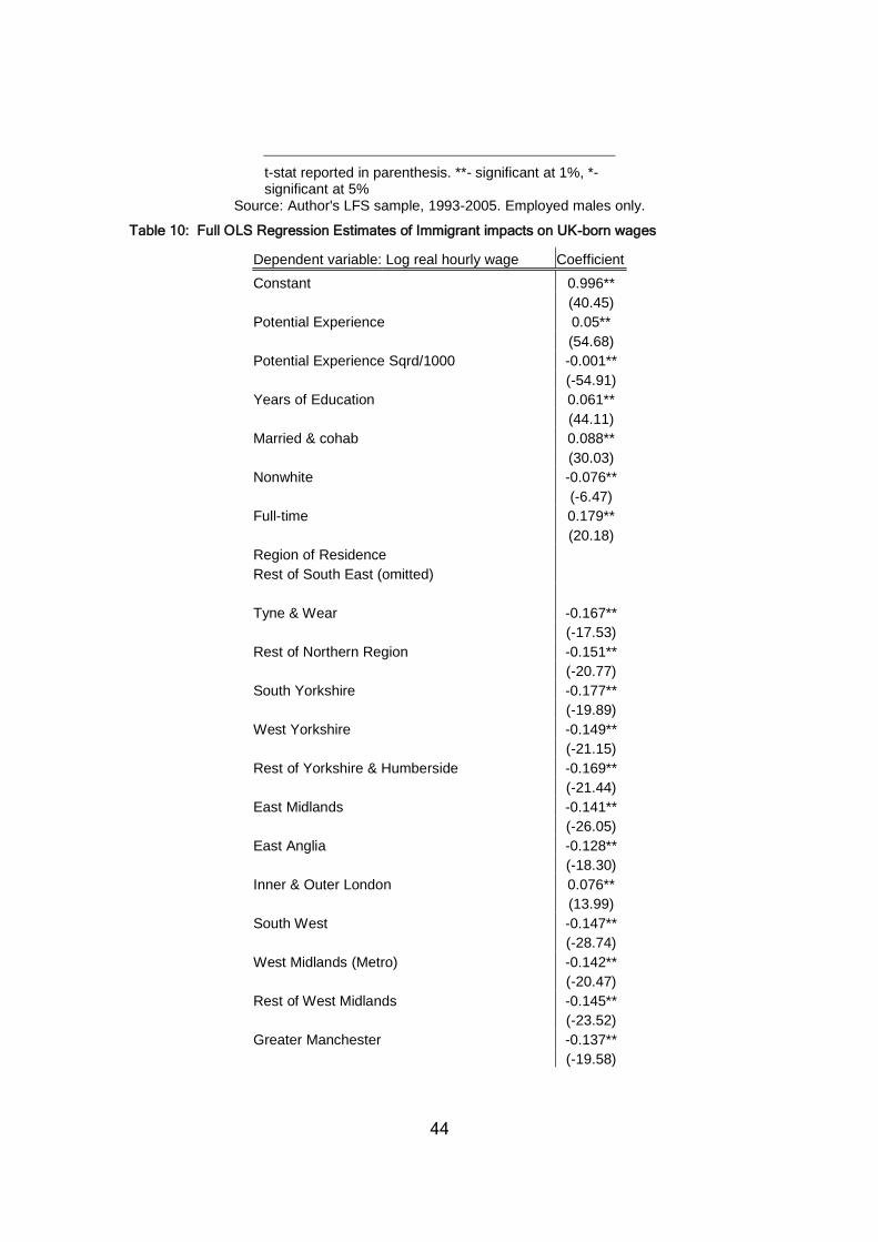
44

t-stat reported in parenthesis. **- significant at 1%, *-significant at 5%

Source: Author's LFS sample, 1993-2005. Employed males only.

Table 10: Full OLS Regression Estimates of Immigrant impacts on UK-born wages

Dependent variable: Log real hourly wage Coefficient

Constant 0.996**

(40.45)

Potential Experience 0.05**

(54.68)

Potential Experience Sqrd/1000 -0.001**

(-54.91)

Years of Education 0.061**

(44.11)

Married & cohab 0.088**

(30.03)

Nonwhite -0.076**

(-6.47)

Full-time 0.179**

(20.18)

Region of Residence

Rest of South East (omitted)

Tyne & Wear -0.167**

(-17.53)

Rest of Northern Region -0.151**

(-20.77)

South Yorkshire -0.177**

(-19.89)

West Yorkshire -0.149**

(-21.15)

Rest of Yorkshire & Humberside -0.169**

(-21.44)

East Midlands -0.141**

(-26.05)

East Anglia -0.128**

(-18.30)

Inner & Outer London 0.076**

(13.99)

South West -0.147**

(-28.74)

West Midlands (Metro) -0.142**

(-20.47)

Rest of West Midlands -0.145**

(-23.52)

Greater Manchester -0.137**

(-19.58)

45

Merseyside -0.157**

(-15.70)

Rest of North West -0.136**

(-19.83)

Wales -0.198**

(-29.95)

Strathclyde & Rest of Scotland -0.146**

(-29.85)

Industries

Manufacturing (omitted)

Agriculture & Fishing -0.40**

(-24.41)

Energy & Water 0.091**

(6.50)

Construction -0.067**

(-5.77)

Distribution, Hotels & Restaurants -0.248**

(-20.80)

Transport & Communication -0.082**

(-6.70)

Banking, Finance & Insurance etc 0.038**

(3.14)

Public admin, Educ & Health -0.073**

(-6.19)

Other Services -0.163**

(-13.72)

Foreign variables

Native skill Immigrant share, by skill

LL LL 0.028*

(2.55)

LM 0.014*

(2.43)

ML 0.021

(1.84)

MM 0.00

(0.00)

MH 0.007

(1.38)

HL 0.004

(0.53)

HM 0.004

(0.61)

HH -0.003

(-0.59)

LL LM -0.049

(-1.48)

LM -0.007

46

(-0.42)

ML -0.064

(-1.85)

MM -0.025

(-1.08)

MH -0.036*

(-2.37)

HL -0.033

(-1.33)

HM 0.004

(0.20)

HH -0.037*

(-2.30)

LL LH -0.14**

(-4.18)

LM -0.048**

(-2.94)

ML -0.135**

(-3.59)

MM -0.02

(-0.87)

MH -0.052**

(-2.98)

HL -0.061*

(-2.16)

HM -0.03

(-1.43)

HH -0.059**

(-3.17)

LL ML -0.013

(-1.81)

LM -0.011**

(-2.87)

ML -0.008

(-1.09)

MM 0.001

(0.16)

MH -0.006

(-1.92)

HL -0.004

(-0.71)

HM -0.002

(-0.59)

HH -0.006

(-1.82)

LL MM 0.028**

(4.29)

LM 0.006

47

(1.65)

ML 0.023**

(3.42)

MM 0.005

(1.06)

MH 0.004

(1.41)

HL 0.012*

(2.49)

HM 0.002

(0.62)

HH 0.006

(1.82)

LL MH -0.039**

(-3.65)

LM -0.008

(-1.54)

ML -0.021

(-1.79)

MM 0.005

(0.71)

MH 0.003

(0.52)

HL -0.006

(-0.65)

HM 0.007

(1.08)

HH 0.008

(1.32)

LL HL 0.015**

(2.94)

LM 0.009**

(3.66)

ML 0.017**

(3.17)

MM 0.008*

(2.22)

MH 0.011**

(4.45)

HL 0.011**

(2.74)

HM 0.005

(1.67)

HH 0.013**

(4.96)

LL HM 0.015**

(3.40)

LM 0.005

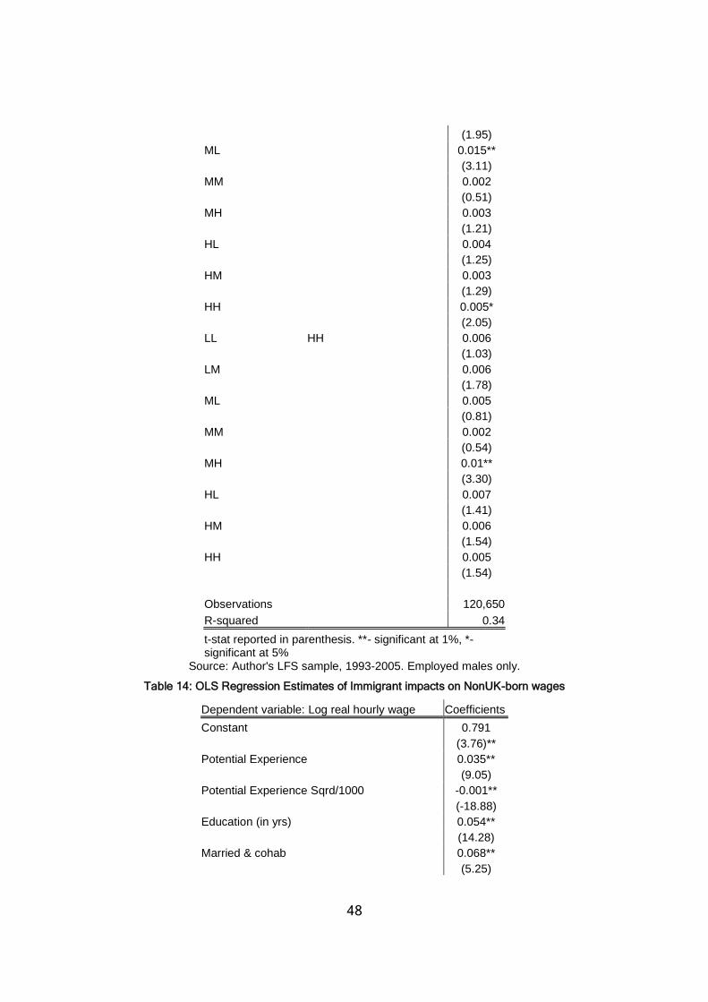
48

(1.95)

ML 0.015**

(3.11)

MM 0.002

(0.51)

MH 0.003

(1.21)

HL 0.004

(1.25)

HM 0.003

(1.29)

HH 0.005*

(2.05)

LL HH 0.006

(1.03)

LM 0.006

(1.78)

ML 0.005

(0.81)

MM 0.002

(0.54)

MH 0.01**

(3.30)

HL 0.007

(1.41)

HM 0.006

(1.54)

HH 0.005

(1.54)

Observations 120,650

R-squared 0.34

t-stat reported in parenthesis. **- significant at 1%, *-significant at 5%

Source: Author's LFS sample, 1993-2005. Employed males only.

Table 14: OLS Regression Estimates of Immigrant impacts on NonUK-born wages

Dependent variable: Log real hourly wage Coefficients

Constant 0.791

(3.76)**

Potential Experience 0.035**

(9.05)

Potential Experience Sqrd/1000 -0.001**

(-18.88)

Education (in yrs) 0.054**

(14.28)

Married & cohab 0.068**

(5.25)

49

Nonwhite -0.191**

(-11.66)

Full-time 0.269**

(7.88)

Age at immigration 0.005**

(1.42)

Years since immigrated sqrd 0.00**

(2.85)

Regions of Birth

Ireland (omitted)

Caribbean&West Indies -0.022**

(-0.60)

China/HK -0.032**

(-0.68)

Europe -0.076**

(-3.30)

India 0.011**

(0.36)

Pakistan/Bangladesh -0.091**

(-2.45)

Old Commonwealth & US 0.086**

(3.52)

Rest of the World -0.062**

(-2.89)

Cohort of Entry to UK

pre-1955 (omitted)

1956-1960 0.069**

(1.79)

1961-1965 0.032**

(-0.70)

1966-1970 0.011**

(0.19)

1971-1975 -0.009**

(-0.13)

1976-1980 -0.039**

(-0.47)

1981-1985 -0.069**

(-0.72)

1986-1990 -0.081**

(-0.74)

1991-1995 -0.111**

(-0.91)

1996-2000 -0.098**

(-0.72)

2001-2005 -0.211**

(-1.42)

50

Region of Residence

Rest of South East (omitted)

Tyne & Wear -0.187**

(2.91)

Rest of Northern Region -0.089**

(-1.67)

South Yorkshire -0.204**

(-3.71)

West Yorkshire -0.233**

(-7.10)

Rest of Yorkshire & Humberside -0.141**

(-3.03)

East Midlands -0.16**

(-6.09)

East Anglia -0.085**

(-2.78)

Inner & Outer London 0.049**

(3.15)

South West -0.137**

(-5.69)

West Midlands (Metro) -0.143**

(-5.34)

Rest of West Midlands -0.087**

(-2.47)

Greater Manchester -0.17**

(-4.91)

Merseyside -0.191**

(-2.79)

Rest of North West -0.088**

(-2.19)

Wales -0.092**

(-2.28)

Strathclyde & Rest of Scotland -0.101**

(-3.52)

Industries

Manufacturing (omitted)

Agriculture & Fishing -0.203**

(-2.03)

Energy & Water 0.19**

(2.54)

Construction 0.00**

(0.01)

Distribution, Hotels & Restaurants -0.258**

(-4.30)

Transport & Communication 0.005**

(0.08)

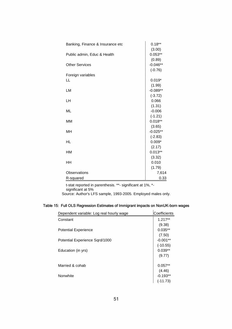
51

Banking, Finance & Insurance etc 0.18**

(3.00)

Public admin, Educ & Health 0.053**

(0.89)

Other Services -0.046**

(-0.76)

Foreign variables

LL 0.019*

(1.99)

LM -0.089**

(-3.72)

LH 0.066

(1.31)

ML -0.006

(-1.21)

MM 0.018**

(3.65)

MH -0.025**

(-2.83)

HL 0.009*

(2.17)

HM 0.013**

(3.32)

HH 0.010

(1.79)

Observations 7,614

R-squared 0.33

t-stat reported in parenthesis. **- significant at 1%, *-significant at 5%

Source: Author's LFS sample, 1993-2005. Employed males only.

Table 15: Full OLS Regression Estimates of Immigrant impacts on NonUK-born wages

Dependent variable: Log real hourly wage Coefficients

Constant 1.217**

(9.38)

Potential Experience 0.035**

(7.50)

Potential Experience Sqrd/1000 -0.001**

(-10.55)

Education (in yrs) 0.039**

(9.77)

Married & cohab 0.057**

(4.46)

Nonwhite -0.193**

(-11.73)

52

Full-time 0.273**

(8.03)

Age at immigration 0.00

(0.06)

Years since immigrated sqrd 0.00**

(2.56)

Regions of Birth

Ireland (omitted)

Caribbean&West Indies -0.005

(-0.14)

China/HK -0.028

(-0.60)

Europe -0.061**

(-2.69)

India 0.016

(0.53)

Pakistan/Bangladesh -0.074

(-2.00)

Old Commonwealth & US 0.098**

(3.99)

Rest of the World -0.056**

(-2.59)

Cohort of Entry to UK

pre-1955 (omitted)

1956-1960 0.106**

(2.98)

1961-1965 0.09**

(2.25)

1966-1970 0.089

(1.87)

1971-1975 0.089

(1.57)

1976-1980 0.081

(1.22)

1981-1985 0.072

(0.93)

1986-1990 0.077

(0.88)

1991-1995 0.063

(0.64)

1996-2000 0.097

(0.89)

2001-2005 -0.015

(-0.13)

53

Region of Residence

Rest of South East (omitted)

Tyne & Wear -0.193**

(-3.01)

Rest of Northern Region -0.077

(-1.44)

South Yorkshire -0.184**

(-3.36)

West Yorkshire -0.226**

(-6.88)

Rest of Yorkshire & Humberside -0.13**

(-2.79)

East Midlands -0.155**

(-5.89)

East Anglia -0.077

(-2.50)

Inner & Outer London 0.041**

(2.65)

South West -0.13**

(-5.39)

West Midlands (Metro) -0.139**

(-5.19)

Rest of West Midlands -0.083

(-2.37)

Greater Manchester -0.174**

(-5.01)

Merseyside -0.194**

(-2.85)

Rest of North West -0.075

(-1.86)

Wales -0.09

(-2.25)

Strathclyde & Rest of Scotland -0.099**

(-3.47)

Industries

Manufacturing (omitted)

Agriculture & Fishing -0.22**

(-2.25)

Energy & Water 0.18**

(2.48)

Construction -0.011

(-0.19)

Distribution, Hotels & Restaurants -0.267**

(-4.66)

Transport & Communication 0.001

54

(0.02)

Banking, Finance & Insurance etc 0.162**

(2.84)

Public admin, Educ & Health 0.039

(0.69)

Other Services -0.055

(-0.95)

Foreign variables

Immigrant skill Immigrant share, by skill

LL LL 0.176*

(2.04)

LM 0.065

(1.79)

ML -0.035

(-0.59)

MM 0.066*

(2.31)

MH 0.041*

(2.05)

HL 0.017

(0.69)

HM 0.019

(1.12)

HH 0.011

(0.69)

LL LM 0.284

(1.20)

LM 0.102

(0.96)

ML -0.119

(-0.60)

MM -0.09

(-1.07)

MH -0.011

(-0.19)

HL 0.019

(0.27)

HM -0.066

(-1.42)

HH -0.129**

(-2.76)

LL LH 0.06

(0.22)

LM 0.015

(0.14)

ML -0.027

(-0.12)

MM 0.115

55

(1.18)

MH 0.059

(0.84)

HL 0.01

(0.12)

HM 0.120*

(2.00)

HH 0.02

(0.33)

LL ML -0.028

(0.53)

LM 0.004

(0.18)

ML -0.012

(-0.28)

MM -0.009

(-0.49)

MH 0.001

(0.05)

HL -0.007

(-0.49)

HM 0.002

(0.18)

HH 0.005

(0.48)

LL MM 0.058

(1.32)

LM 0.010

(0.47)

ML -0.017

(-0.47)

MM 0.023

(1.45)

MH 0.001

(0.08)

HL 0.001

(0.10)

HM 0.030**

(3.14)

HH 0.02*

(2.15)

LL MH 0.018

(0.19)

LM -0.042

(-1.19)

ML -0.067

(-0.87)

MM -0.082**

56

(-2.73)

MH -0.035

(-1.57)

HL 0.001

(0.03)

HM -0.052**

(-2.81)

HH -0.022

(-1.16)

LL HL 0.018

(0.48)

LM -0.003

(-0.17)

ML 0.062*

(1.96)

MM 0.029*

(2.02)

MH 0.006

(0.65)

HL 0.002

(0.18)

HM -0.005

(-0.59)

HH 0.007

(0.83)

LL HM -0.058

(-1.79)

LM -0.014

(-0.90)

ML 0.023

(0.85)

MM -0.011

(-0.92)

MH 0.000

(0.05)

HL 0.011

(1.07)

HM 0.013

(1.91)

HH 0.007

(1.00)

LL HH -0.097

(-1.81)

LM -0.001

(-0.06)

ML -0.011

(-0.31)

MM 0.007

57

(0.38)

MH -0.001

(-0.04)

HL -0.016

(-1.05)

HM 0.000

(0.03)

HH 0.018

(1.68)

Observations 7,614

R-squared 0.35

t-stat reported in parenthesis. **- significant at 1%, *- significant at5%

Source: Author's LFS sample, 1993-2005. Employed males only.

Table 116: Full Quantile Regression Estimates for UK-born

Quantiles

Dependent variable: Log real hourly wage 0.10 0.25 0.50 0.75 0.90

Constant 0.183** 0.283** 0.485** 0.785** 1.119**

(3.24) (6.00) (11.14) (16.25) (16.17)

Potential Experience 0.048** 0.051** 0.055** 0.057** 0.058**

(105.51) (116.32) (144.06) (136.85) (57.63)

Potential Experience Sqrd/1000 -0.001** -0.001** -0.001** -0.001** -0.001**

(-85.56) (-118.61) (-107.68) (-111.29) (-46.33)

Years of Education 0.075** 0.079** 0.08** 0.08** 0.083**

(98.87) (105.75) (141.05) (114.72) (106.06)

Married & cohab 0.104** 0.099** 0.094** 0.087** 0.09**

(26.22) (30.46) (25.23) (22.43) (18.10)

Nonwhite -0.064** -0.09** -0.063** -0.075** -0.073**

(-3.03) (-5.31) (-4.76) (-4.86) (-3.47)

Full-time 0.295** 0.259** 0.208** 0.127** 0.025**

(21.29) (20.55) (22.45) (11.13) (1.06)

Region of Residence

Rest of South East (omitted)

Tyne & Wear -0.134** -0.158** -0.169** -0.184** -0.214**

(-7.64) (-13.33) (-13.27) (-18.17) (-10.73)

Rest of Northern Region -0.141** -0.155** -0.147** -0.156** -0.169**

(-12.42) (-18.06) (-20.54) (-16.36) (-12.52)

South Yorkshire -0.145** -0.142** -0.163** -0.195** -0.234**

(-13.54) (-11.08) (-18.79) (-24.45) (-20.14)

West Yorkshire -0.103** -0.132** -0.15** -0.171** -0.196**

(-11.24) (-14.94) (-18.62) (-20.01) (-17.17)

Rest of Yorkshire & Humberside -0.165** -0.167** -0.157** -0.172** -0.186**

(-12.82) (-17.57) (-22.28) (-18.33) (-16.45)

58

East Midlands -0.094** -0.126** -0.143** -0.159** -0.17**

(-11.46) (-21.83) (-39.67) (-30.02) (-19.68)

East Anglia -0.079** -0.112** -0.133** -0.143** -0.149**

(-9.68) (-14.68) (-15.33) (-11.70) (-12.50)

Inner & Outer London 0.083** 0.08** 0.081** 0.082** 0.09**

(8.92) (11.81) (14.39) (11.61) (9.85)*

South West -0.119** -0.131** -0.14** -0.158** -0.174**

(-14.06) (-22.55) (-21.23) (-20.40) (-18.43)

West Midlands (Metro) -0.101** -0.114** -0.136** -0.163** -0.189**

(-7.23) (-13.13) (-18.69) (-17.22) (-15.98)

Rest of West Midlands -0.098** -0.13** -0.148** -0.17** -0.196**

(-13.58) (-20.12) (-23.55) (-24.41) (-25.78)

Greater Manchester -0.112** -0.12** -0.137** -0.154** -0.187**

(-11.91) (-14.62) (-17.21) (-18.82) (-19.80)

Merseyside -0.124** -0.126** -0.151** -0.185** -0.195**

(-6.21) (-12.14) (-18.03) (-16.88) (-14.20)

Rest of North West -0.117** -0.121** -0.119** -0.138** -0.154**

(-9.49) (-15.07) (-19.26) (-26.80) (-14.45)

Wales -0.169** -0.185** -0.193** -0.207** -0.221**

(-15.13) (-24.31) (-32.77) (-25.08) (-17.35)

Strathclyde & Rest of Scotland -0.119** -0.135** -0.146** -0.152** -0.166**

(-22.03) (-21.91) (-31.70) (-21.91) (-19.58)

Industries

Manufacturing (omitted)

Agriculture & Fishing -0.348** -0.364** -0.367** -0.397** -0.422**

(-12.69) (-18.56) (-18.72) (-22.74) (-22.88)

Energy & Water 0.124** 0.099** 0.099** 0.098** 0.085**

(5.61) (5.33) (6.63) (6.71) (3.27)

Construction -0.055** -0.052** -0.036** -0.061** -0.086**

(-2.80) (-3.29) (-2.65) (-4.09) (-4.44)

Distribution, Hotels & Restaurants -0.254** -0.25** -0.229** -0.232** -0.217**

(-13.43) (-15.83) (-19.39) (-17.18) (-10.93)

Transport & Communication -0.059** -0.061** -0.057** -0.082** -0.085**

(-3.08) (-3.88) (-5.05) (-5.85) (-4.20)

Banking, Finance & Insurance etc -0.038** 0.021** 0.077** 0.098** 0.115**

(-2.26) (1.47) (6.18) (6.11) (6.59)

Public admin, Educ & Health -0.04** -0.031** -0.026** -0.074** -0.138**

(-2.24) (-2.02) (-1.87) (-5.19) (-7.38)

Other Services -0.157** -0.157** -0.138** -0.153** -0.162**

(-7.78) (-9.85) (-9.88) (-9.36) (-6.90)

Foreign Variables

LL 0.009** 0.004* 0.004* 0.001 0.00

(3.65) (2.26) (2.39) (0.42) (0.10)

LM -0.008 -0.022** -0.016** -0.024** -0.014

(-1.11) (-3.52) (-3.41) (-3.83) (-1.63)

LH -0.034* -0.01 0.001 0.014 0.007

(-2.55) (-0.76) (0.10) (1.24) (0.34)

59

ML -0.004* -0.004* -0.003* -0.001 -0.002

(-2.07) (-2.41) (-2.17) (-0.56) (-0.82)

MM 0.006** 0.004** 0.003* 0.005** 0.005*

(2.65) (2.75) (2.46) (3.71) (2.57)

MH -0.002 0.001 0.002 -0.001 0.003

(-0.69) (0.65) (1.14) (-0.24) (0.91)

HL 0.01** 0.01** 0.009** 0.007** 0.008**

(6.69) (10.46) (8.58) (6.58) (4.23)

HM 0.002 0.004** 0.003** 0.005** 0.003**

(1.45) (5.57) (5.09) (5.38) (2.68)

HH 0.002 0.005** 0.005** 0.006** 0.005**

(1.47) (3.71) (5.47) (4.75) (3.30)

Observations 120,650

Pseudo R-squared 0.181 0.207 0.221 0.219 0.207

t-stat reported in parenthesis. **- significant at 1%, *- significant at 5%Source: Author's LFS sample, 1993-2005. Employed males only.

Table 12: Full Quantile Regression Estimates for NonUK-born

Quantiles

Dependent variable: Log real hourly wage 0.10 0.25 0.50 0.75 0.90

Constant 0.185 0.625** 0.597** 0.863** 1.151**

(0.62) (3.03) (2.67) (3.21) (2.91)

Potential Experience 0.033** 0.035** 0.039** 0.039** 0.043**

(4.89) (10.11) (9.66) (9.32) (6.88)

Potential Experience Sqrd/1000 -0.001** -0.001** -0.001** -0.001** -0.001**

(-9.09) (-14.80) (-18.16) (-16.44) (-11.07)

Education (in yrs) 0.053** 0.055** 0.058** 0.058** 0.061**

(7.06) (14.32) (11.55) (10.84) (8.57)

Married & cohab 0.071** 0.068** 0.065** 0.057** 0.062*

(3.29) (4.29) (4.45) (2.76) (2.01)

Nonwhite -0.195** -0.197** -0.187** -0.188** -0.179**

(-9.14) (-10.68) (-11.29) (-7.89) (-7.32)

Full-time 0.325** 0.303** 0.263** 0.225** 0.115**

(4.38) (7.87) (6.25) (3.97) (1.85)

Age at immigration -0.006** -0.001** 0.002** 0.01** 0.011**

(-0.95) (-0.28) (0.42) (2.60) (1.98)

Years since immigrated sqrd 0.00 0.00** 0.00 0.00** 0.00*

(0.06) (2.64) (1.29) (3.14) (2.17)

Regions of Birth

Ireland (omitted)

Caribbean&West Indies 0.026 0.015 -0.02 -0.009 -0.076

(0.68) (0.54) (-0.54) (-0.17) (-1.56)

China/HK -0.006 -0.044 -0.036 -0.085 -0.043

(-0.07) (-1.00) (-0.91) (-1.46) (-0.57)

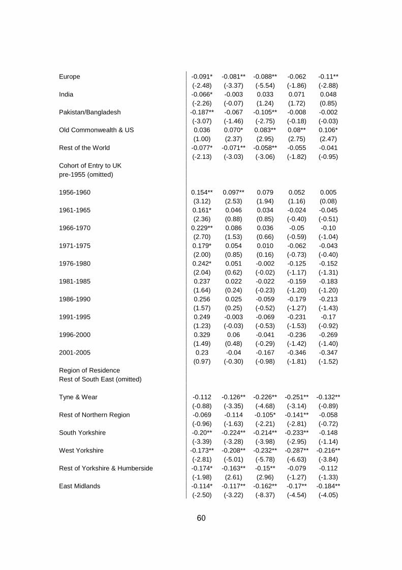
60

Europe -0.091* -0.081** -0.088** -0.062 -0.11**

(-2.48) (-3.37) (-5.54) (-1.86) (-2.88)

India -0.066* -0.003 0.033 0.071 0.048

(-2.26) (-0.07) (1.24) (1.72) (0.85)

Pakistan/Bangladesh -0.187** -0.067 -0.105** -0.008 -0.002

(-3.07) (-1.46) (-2.75) (-0.18) (-0.03)

Old Commonwealth & US 0.036 0.070* 0.083** 0.08** 0.106*

(1.00) (2.37) (2.95) (2.75) (2.47)

Rest of the World -0.077* -0.071** -0.058** -0.055 -0.041

(-2.13) (-3.03) (-3.06) (-1.82) (-0.95)

Cohort of Entry to UK

pre-1955 (omitted)

1956-1960 0.154** 0.097** 0.079 0.052 0.005

(3.12) (2.53) (1.94) (1.16) (0.08)

1961-1965 0.161* 0.046 0.034 -0.024 -0.045

(2.36) (0.88) (0.85) (-0.40) (-0.51)

1966-1970 0.229** 0.086 0.036 -0.05 -0.10

(2.70) (1.53) (0.66) (-0.59) (-1.04)

1971-1975 0.179* 0.054 0.010 -0.062 -0.043

(2.00) (0.85) (0.16) (-0.73) (-0.40)

1976-1980 0.242* 0.051 -0.002 -0.125 -0.152

(2.04) (0.62) (-0.02) (-1.17) (-1.31)

1981-1985 0.237 0.022 -0.022 -0.159 -0.183

(1.64) (0.24) (-0.23) (-1.20) (-1.20)

1986-1990 0.256 0.025 -0.059 -0.179 -0.213

(1.57) (0.25) (-0.52) (-1.27) (-1.43)

1991-1995 0.249 -0.003 -0.069 -0.231 -0.17

(1.23) (-0.03) (-0.53) (-1.53) (-0.92)

1996-2000 0.329 0.06 -0.041 -0.236 -0.269

(1.49) (0.48) (-0.29) (-1.42) (-1.40)

2001-2005 0.23 -0.04 -0.167 -0.346 -0.347

(0.97) (-0.30) (-0.98) (-1.81) (-1.52)

Region of Residence

Rest of South East (omitted)

Tyne & Wear -0.112 -0.126** -0.226** -0.251** -0.132**

(-0.88) (-3.35) (-4.68) (-3.14) (-0.89)

Rest of Northern Region -0.069 -0.114 -0.105* -0.141** -0.058

(-0.96) (-1.63) (-2.21) (-2.81) (-0.72)

South Yorkshire -0.20** -0.224** -0.214** -0.233** -0.148

(-3.39) (-3.28) (-3.98) (-2.95) (-1.14)

West Yorkshire -0.173** -0.208** -0.232** -0.287** -0.216**

(-2.81) (-5.01) (-5.78) (-6.63) (-3.84)

Rest of Yorkshire & Humberside -0.174* -0.163** -0.15** -0.079 -0.112

(-1.98) (2.61) (2.96) (-1.27) (-1.33)

East Midlands -0.114* -0.117** -0.162** -0.17** -0.184**

(-2.50) (-3.22) (-8.37) (-4.54) (-4.05)

61

East Anglia -0.087 -0.065 -0.08* -0.078 -0.071

(-1.16) (-1.48) (-2.53) (-1.77) (-1.28)

Inner & Outer London 0.062** 0.069** 0.052** 0.052** 0.056**

(2.45) (3.27) (3.79) (2.80) (1.65)

South West -0.153** -0.138** -0.143** -0.122** -0.096*

(-2.62) (-5.11) (-7.40) (-2.99) (-1.99)

West Midlands (Metro) -0.092** -0.08* -0.141** -0.127** -0.166**

(-3.00) (-2.25) (-5.38) (-3.84) (-3.53)

Rest of West Midlands -0.03 -0.071* -0.101** -0.11** -0.099

(-0.66) (-1.96) (-2.99) (-3.08) (-1.49)

Greater Manchester -0.248** -0.197** -0.16** -0.114** -0.104

(-4.02) (-7.05) (-4.43) (-2.69) (-1.22)

Merseyside -0.184* -0.175** -0.255** -0.172 -0.22

(-1.97) (-4.01) (-2.65) (-1.55) (-1.86)

Rest of North West -0.121 -0.145** -0.08 -0.048 -0.043

(-1.80) (-2.68) (-1.65) (-0.69) (-0.51)

Wales -0.057 -0.099 -0.152** -0.094 -0.066

(-0.96) (-1.87) (-4.93) (-1.47) (-0.73)

Strathclyde & Rest of Scotland -0.095* -0.117** -0.106** -0.093 -0.108

(-2.01) (-3.06) (-3.61) (-1.88) (-1.83)

Industries

Manufacturing (omitted)

Agriculture & Fishing -0.467** -0.318** -0.225* -0.182 -0.225

(-2.85) (-2.59) (-2.08) (-1.47) (-0.84)

Energy & Water 0.261* 0.137 0.194** 0.213** 0.152**

(1.97) (1.46) (2.76) (2.85) (1.84)

Construction -0.035 -0.062 -0.02 0.036 0.021

(-0.27) (-0.71) (-0.37) (-0.78) (-0.54)

Distribution, Hotels & Restaurants -0.297* -0.31** -0.266** -0.231** -0.201**

(-2.11) (-3.58) (-4.61) (-4.28) (-4.63)

Transport & Communication 0.012 -0.003 -0.006 0.013 -0.042

(0.09) (-0.04) (-0.11) (0.24) (-0.76)

Banking, Finance & Insurance etc 0.068 0.113 0.171** 0.258** 0.293**

(0.55) (1.28) (2.86) (5.06) (5.73)

Public admin, Educ & Health 0.068 0.058 0.058 0.043 -0.028

(0.51) (0.70) (1.08) (0.93) (-0.54)

Other Services -0.063 -0.102 -0.074 -0.011 0.004

(-0.45) (-1.27) (-1.23) (-0.20) (0.09)

Foreign variables

LL 0.015 0.021 0.017 0.018 0.007

(0.79) (1.44) (1.68) (1.51) (0.42)

LM -0.067* -0.084* -0.102** -0.106** -0.125*

(-1.97) (-2.70) (-4.43) (-2.94) (-2.36)

LH 0.114 0.044 0.098* 0.074 -0.009

(1.47) (0.73) (2.21) (1.16) (-0.09)

ML 0.003 0.001 -0.002 -0.013 -0.022

(0.28) (0.07) (-0.52) (-1.95) (-1.90)

62

MM 0.014 0.012 0.018** 0.018** 0.017*

(1.76) (1.92) (3.57) (3.15) (2.23)

MH -0.03* -0.019* -0.016 -0.027* -0.012

(-2.43) (-2.17) (-1.22) (-2.52) (-0.71)

HL 0.003 0.011* 0.007 0.015** 0.02**

(0.42) (2.01) (1.48) (2.93) (2.73)

HM 0.011* 0.008* 0.014** 0.014* 0.021**

(2.22) (1.98) (3.36) (2.51) (3.16)

HH 0.003 0.005 0.009 0.019* 0.023*

(0.35) (0.58) (1.47) (2.37) (2.03)

Observations 7,614

Pseudo R-squared 0.155 0.197 0.221 0.221 0.228

t-stat reported in parenthesis. **- significant at 1%, *- significant at 5%Source: Author's LFS sample, 1993-2005. Employed males only.

63

CSGR Working Paper Series

212/06 October Peter Waterman and Kyle PopeThe Bamako Appeal of Samir Amin: A Post-Modern Janus?

213/06 October Marcus Miller, Javier García-Fronti and Lei ZhangSupply Shocks and Currency Crises: The Policy Dilemma Reconsidered

214/06 December Gianluca GrimaldaWhich Relation between Globalisation and Individual Propensity toCo-Operate? Some Preliminary Results from an ExperimentalInvestigation

215/07 January Kui-Wai Li, Iris A.J. Pang and Michael C.M. NgCan Performance of Indigenous Factors Influence Growth andGlobalisation?

216/06 December Marcus Miller and Lei ZhangFear and Market Failure: Global Imbalances and “Self-insurance”

217/07 February Catherine HoskynsLinking Gender and International Trade Policy: Is Interaction Possible?

218/07 February Dilip K. DasSouth Asian Free Trade Agreement: Prospects of Shallow RegionalIntegration

219/07 February Vanesa WeyrauchWeaving Global Networks: Handbook for Policy Influence

220/07 February Yuji TamuraPreferences for Immigration Restriction and Opinions about Immigrant’sEconomic Impacts

221/07 March Dania Thomas and Javier García-FrontiGood Faith in Sovereign Debt Restructuring: The Evolution of an OpenNorm in ‘Localised’ Contexts?

222/07 March Michela RedoanoFiscal Interactions Among European Countries: Does the EU Matter?

223/07 March Jan Aart ScholteCivil Society and the Legitimation of Global Governance

224/07 March Dwijen RangnekarContext and Ambiguity: A Comment on Amending India’s Patent Act

225/07 May Marcelo I. SaguierGlobal Governance and the HIV/AIDS Response: Limitations of CurrentApproaches and Policies

226/07 May Dan BulleyExteriorising Terror: Inside/Outside the Failing State on 7 July 2005

64

227/07 May Kenneth AmaeshiWho Matters to UK and German Firms? Modelling Stakeholder SalienceThrough Corporate Social Reports

228/07 May Olufemi O. Amao and Kenneth M. AmaeshiGalvanising Shareholder Activism: A Prerequisite for Effective CorporateGovernance and Accountability in Nigeria

229/07 June Stephen J. Redding, Daniel M. Sturm and Nikolaus WolfHistory and Industry Location: Evidence from German Airports

230/07 June Dilip K. DasShifting Paradigm of Regional Integration in Asia

231/07 June Max-Stephan Schulze and Nikolaus WolfOn the Origins of Border Effects: Insights from the Habsburg CustomsUnion

232/07 July Elena Meschi and Marco VivarelliTrade Openness and Income Inequality in Developing Countries

233/07 July Julie GilsonStructuring Accountability: Non-Governmental Participation in the Asia-Europe Meeting (ASEM)

234/07 September Christian Thimann, Christian Just and Raymond RitterThe Governance of the IMF: How a Dual Board Structure Could Raisethe Effectiveness and Legitimacy of a Key Global Institution

235/07 October Peter I. HajnalCan Civil Society Influence G8 Accountability?

236/07 November Ton BührsTowards a Global Political-Economic Architecture of EnvironmentalSpace

Centre for the Study of Globalisation and RegionalisationUniversity of Warwick

Coventry CV4 7AL, UK

Tel: +44 (0)24 7657 2533Fax: +44 (0)24 7657 2548

Email: csgr@warwick.ac.ukWeb address: http://www.csgr.org