Embed Size (px)
Citation preview
HEP data analysis using ROOT
week I ▪ ROOT, CLING and the command line ▪ Histograms, Graphs and Trees
Mark Hodgkinson
Course contents
• ROOT, CLING and the command line • Histograms, Graphs and Trees • File I/O, memory and object ownership • Fitting, peak finding and Fourier analysis • Using Maths and Physics libraries • ROOT geometries • Developing shared libraries • Bindings to other languages • ROOT as a dependence in your application
2
Aims/Objectives
• To work through various HEP use cases – biased by J. Perkins own experience on T2K • slides (mostly) written by J. Perkins
• Not a digest of existing documentation – will signpost useful resources where apt
• To be interactive – problems/exercises each week - not assessed, but I
am supposed to check you tried them! So either we can do this as we go along (only if everyone has a laptop with them) or just email me the output of the tasks (email address at end).
3
About Me
• My own perspective is an ATLAS user and mostly with C++, with some python and a lot of shell scripting.
• Mostly have used ROOT for histograms, fitting of histograms and machine learning (neural net to find K0s particles in BaBar and BDT to distinguish pi0 and hadronic calorimeter clusters in ATLAS).
• Some experiments may have their own additional layers - e.g. ATLAS has its own analysis frameworks which works directly with ATLAS specific c++ objects, some people then convert those formats to TTree (see relevant slides) which can be used outside ATLAS code framework.
4
How to Get Help
• Any relevant mailing lists in your experiment.
• Ask a someone in our HEP group (e.g. who you share an office with).
• Ask on ROOT forums -don’t send them your code. They very often ask for a small self contained and standalone example demonstrating the issue you have, so that they can run it to reproduce your issue.
5
Week 1
• ROOT, CLING and the command line – quick introduction to ROOT and CLING
• Histograms and Graphs – reading, writing and visualising data – formatting and plot aesthetics –writing simple macros
• Trees • This course assumes you are familiar with C++ and
Object Oriented programming - if not, we can divert some (brief) time to explain concepts as they come up. Just ask…
6
ROOT and CINT• Written at CERN, ROOT has been developed
for many years – evolved from many other projects, mainly PAW
(Fortran) • It predates ANSI C++ – Your compiler will complain if you break standards
and conventions • ROOT 5 CINT probably won’t - but we will learn using
ROOT 6 – ROOT 5 CINT contains many relics/implementations
that are not considered good practice today • idiosyncrasies, particularities and peculiarities galore
• ROOT is not the only data analysis package you can use, and some people argue not even close to the best - but it is the most widely used in particle physics. 7
ROOT, CINT and CLING
• CLING (or CINT) is a C/C++ JIT (interpreter) in which lines of code can be executed in similar fashion to a standard ‘nix shell – * not ANSI compliant
• CLING replaced CINT in ROOT6
• CLING (or CINT) is a useful environment in which to manipulate data interactively and develop code – emulation incurs performance overheads so not
suitable for large-scale processing
8
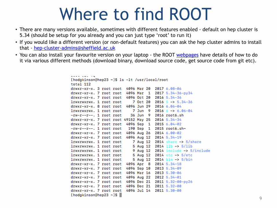
Where to find ROOT • There are many versions available, sometimes with different features enabled - default on hep cluster is
5.34 (should be setup for you already and you can just type ‘root’ to run it) • If you would like a different version (or non-default features) you can ask the hep cluster admins to install
that - [email protected] • You can also install your favourite version on your laptop - the ROOT webpages have details of how to do
it via various different methods (download binary, download source code, get source code from git etc).
9
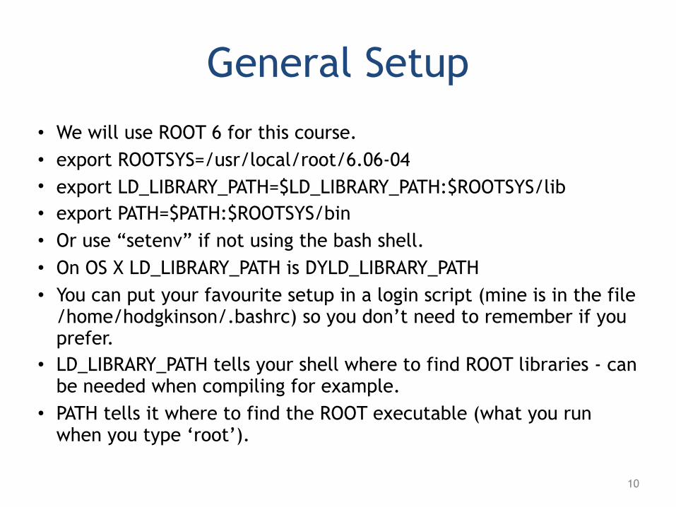
General Setup• We will use ROOT 6 for this course. • export ROOTSYS=/usr/local/root/6.06-04 • export LD_LIBRARY_PATH=$LD_LIBRARY_PATH:$ROOTSYS/lib • export PATH=$PATH:$ROOTSYS/bin • Or use “setenv” if not using the bash shell. • On OS X LD_LIBRARY_PATH is DYLD_LIBRARY_PATH • You can put your favourite setup in a login script (mine is in the file
/home/hodgkinson/.bashrc) so you don’t need to remember if you prefer.
• LD_LIBRARY_PATH tells your shell where to find ROOT libraries - can be needed when compiling for example.
• PATH tells it where to find the ROOT executable (what you run when you type ‘root’).
10
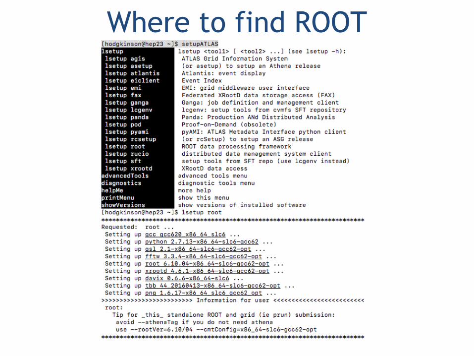
• If you work in a large collaboration they may have a way for you to use a version they recommend.
• For example ATLAS provides the setup (for other experiments you will have to ask colleagues) shown on the next page
Where to find ROOT
Where to find ROOT
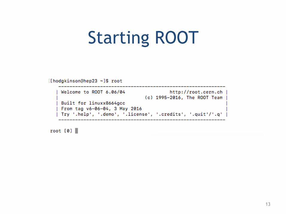
Starting ROOT
13
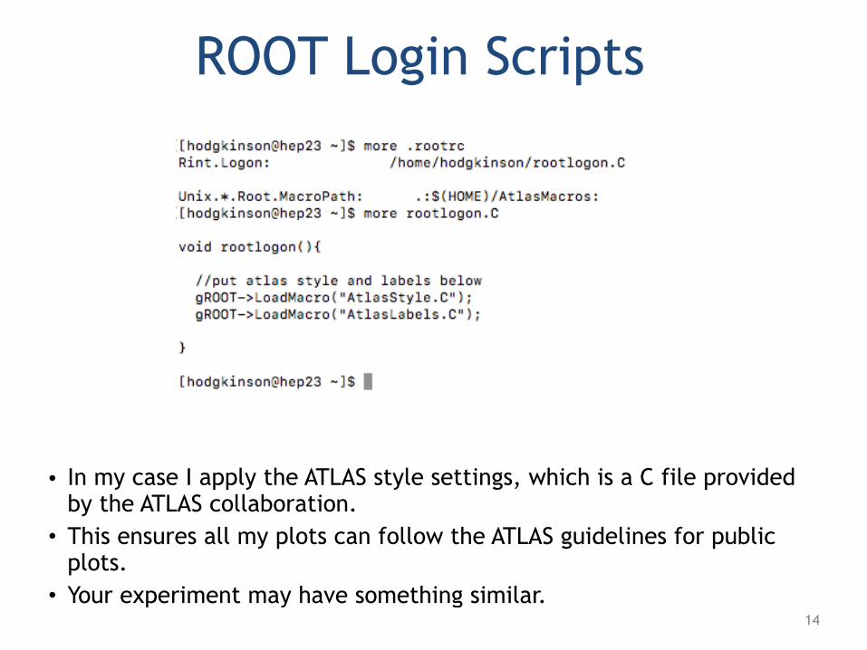
ROOT Login Scripts
• In my case I apply the ATLAS style settings, which is a C file provided by the ATLAS collaboration.
• This ensures all my plots can follow the ATLAS guidelines for public plots.
• Your experiment may have something similar.14
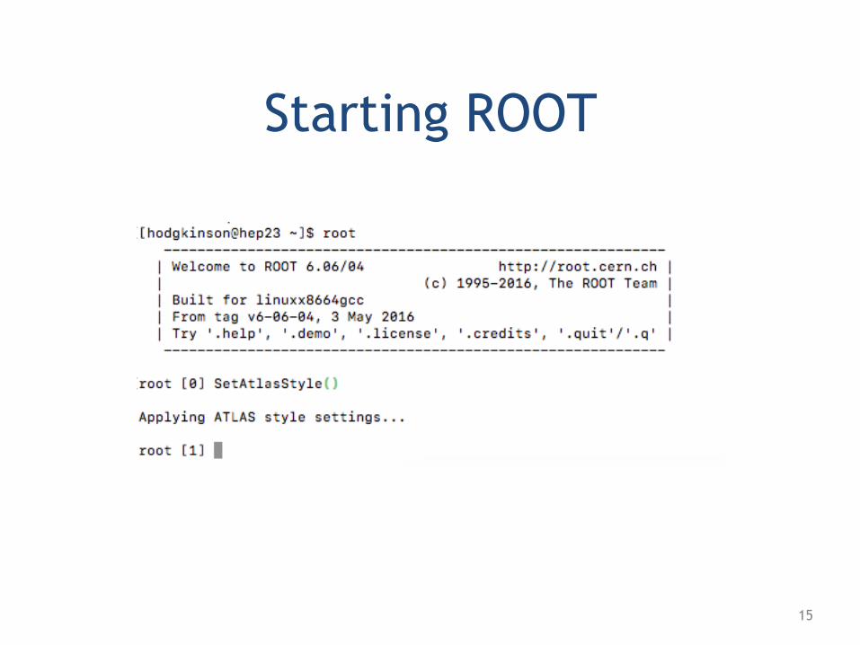
Starting ROOT
15
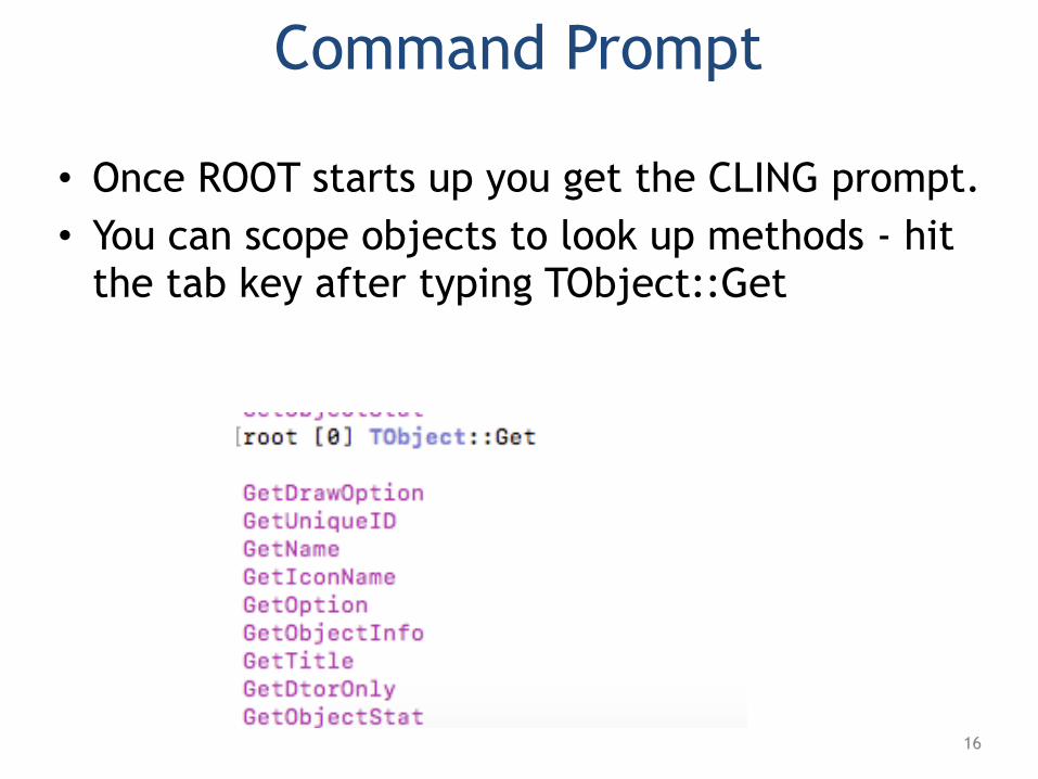
Command Prompt
• Once ROOT starts up you get the CLING prompt. • You can scope objects to look up methods - hit
the tab key after typing TObject::Get
16
Starting ROOT
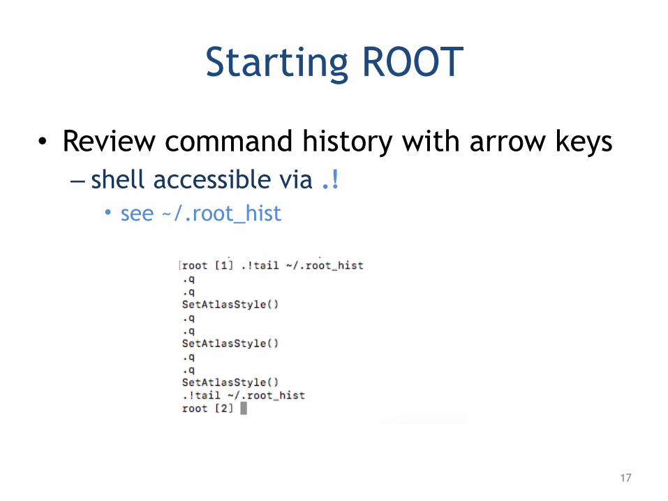
• Review command history with arrow keys – shell accessible via .! • see ~/.root_hist
17
Histograms
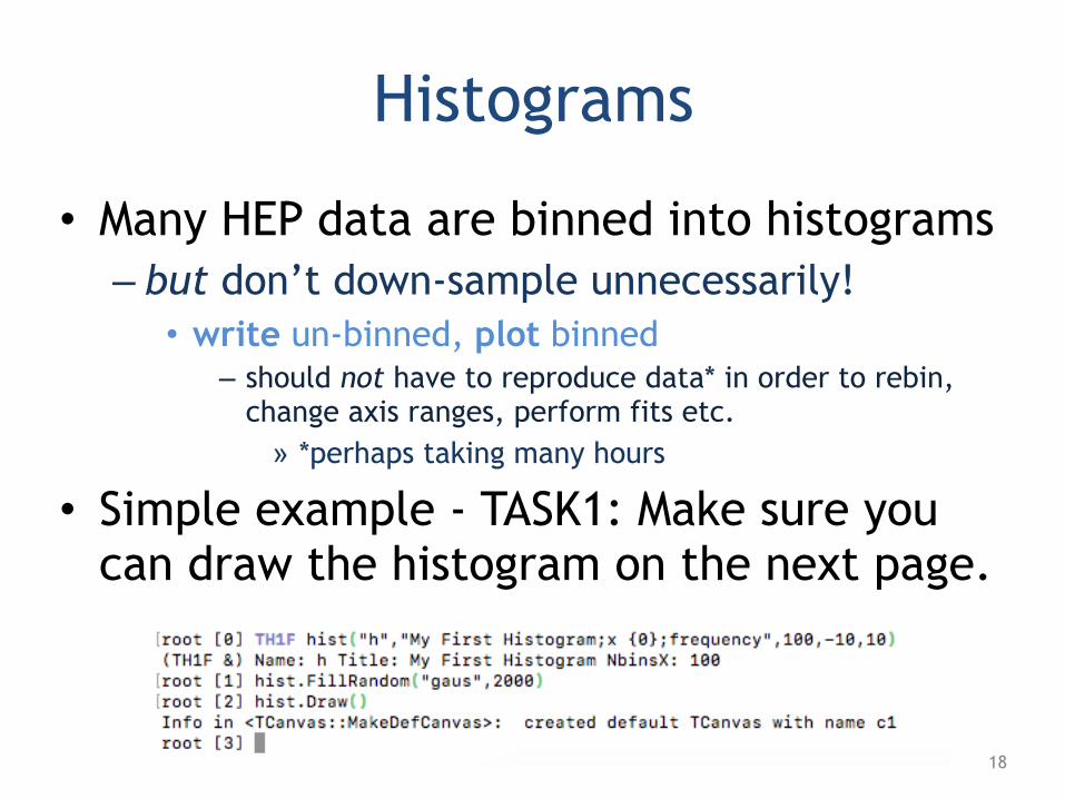
• Many HEP data are binned into histograms – but don’t down-sample unnecessarily! • write un-binned, plot binned
– should not have to reproduce data* in order to rebin, change axis ranges, perform fits etc. » *perhaps taking many hours
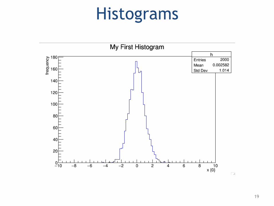
• Simple example - TASK1: Make sure you can draw the histogram on the next page.
18
Histograms
19
Histograms
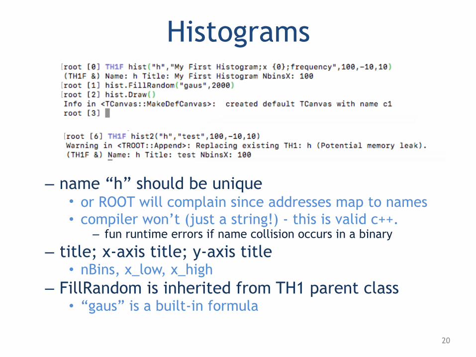
– name “h” should be unique • or ROOT will complain since addresses map to names • compiler won’t (just a string!) - this is valid c++.
– fun runtime errors if name collision occurs in a binary
– title; x-axis title; y-axis title • nBins, x_low, x_high
– FillRandom is inherited from TH1 parent class • “gaus” is a built-in formula
20
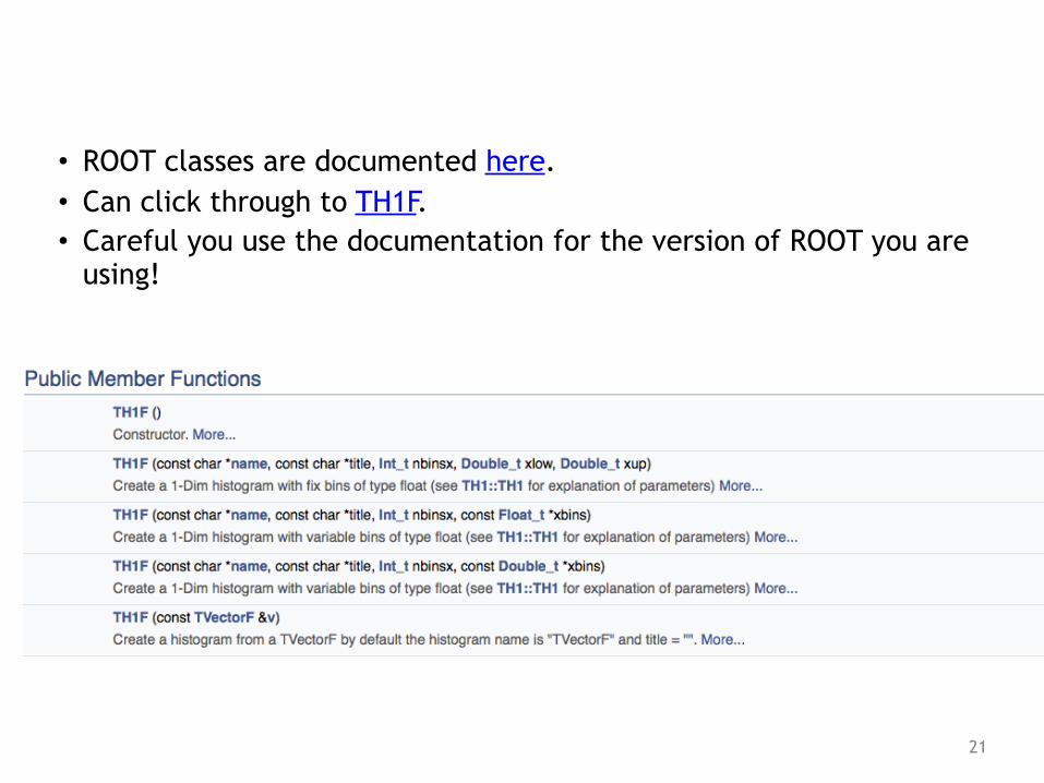
• ROOT classes are documented here. • Can click through to TH1F. • Careful you use the documentation for the version of ROOT you are
using!
21
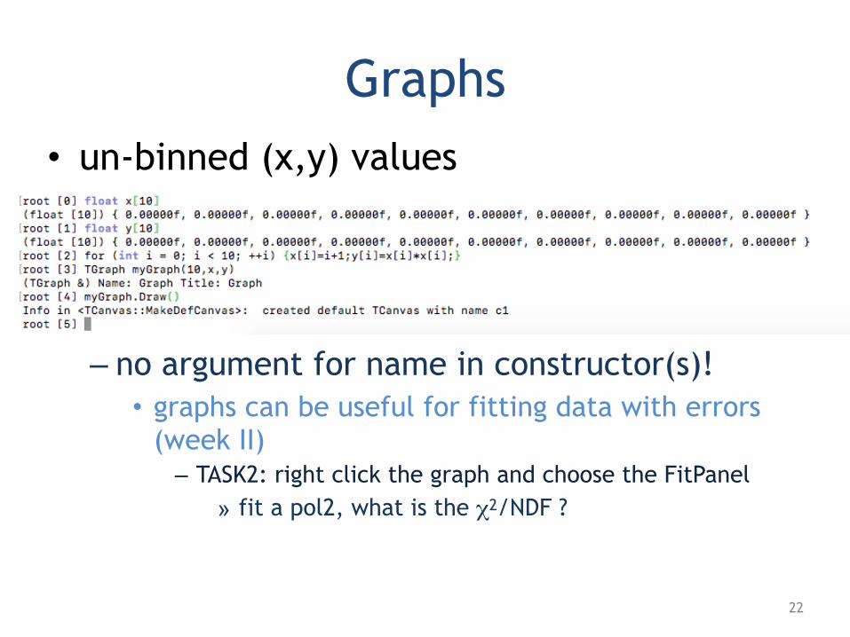
Graphs• un-binned (x,y) values
– no argument for name in constructor(s)! • graphs can be useful for fitting data with errors
(week II) – TASK2: right click the graph and choose the FitPanel
» fit a pol2, what is the χ2/NDF ?
22
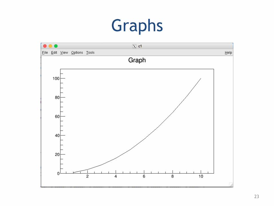
Graphs
23
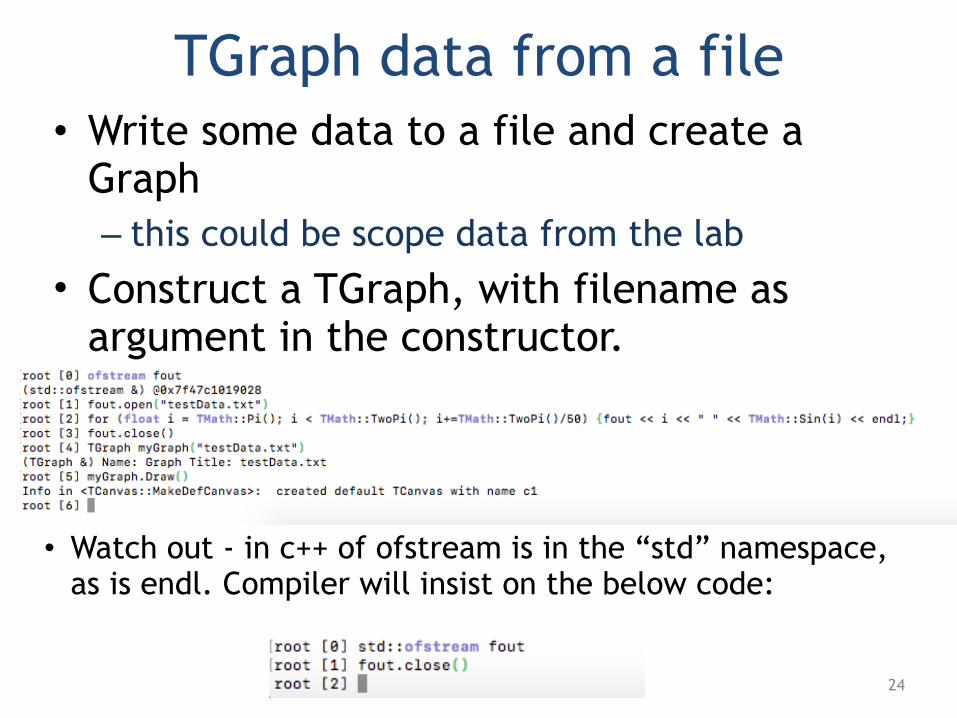
TGraph data from a file• Write some data to a file and create a
Graph – this could be scope data from the lab
• Construct a TGraph, with filename as argument in the constructor.
• Watch out - in c++ of ofstream is in the “std” namespace, as is endl. Compiler will insist on the below code:
24
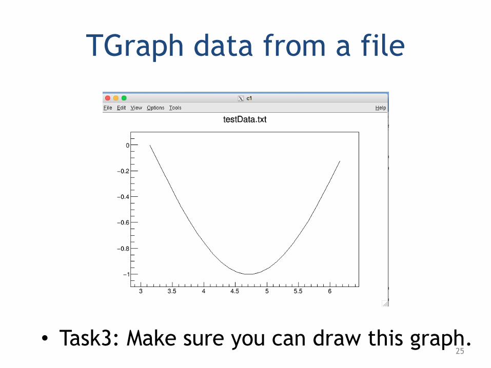
TGraph data from a file
• Task3: Make sure you can draw this graph.25
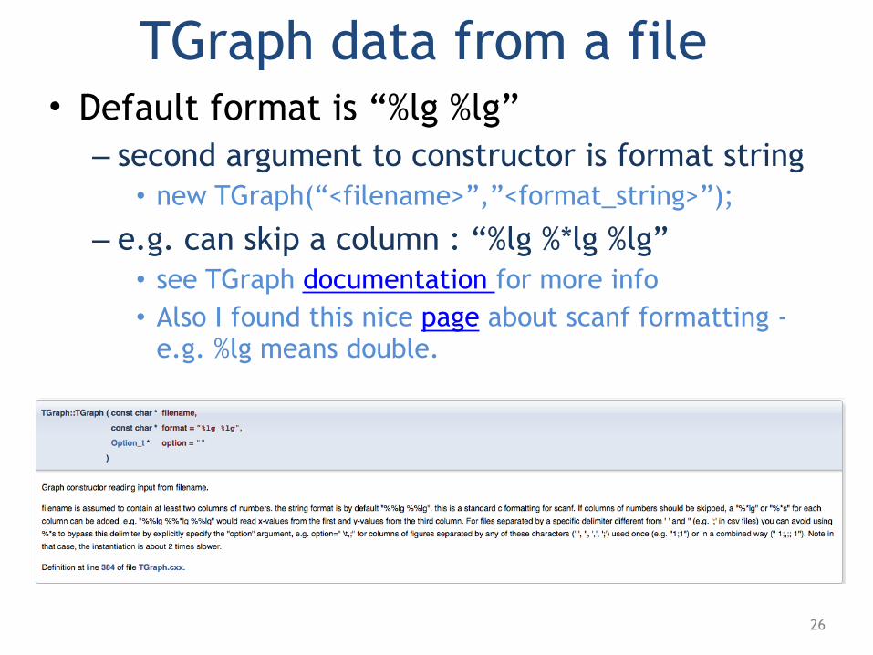
TGraph data from a file• Default format is “%lg %lg” – second argument to constructor is format string
• new TGraph(“<filename>”,”<format_string>”);
– e.g. can skip a column : “%lg %*lg %lg” • see TGraph documentation for more info • Also I found this nice page about scanf formatting -
e.g. %lg means double.
26
Plot aesthetics
• Use the GUI to make your plots nicer – choose Editor from the View menu
• Interactively set (via right click in relevant places) – line widths – colors [sic] – axis titles – grid lines – choose Toolbar from View menu for more features – Use SaveAs *.C to save a file which can regenerate
this plot.
27
ROOT macros
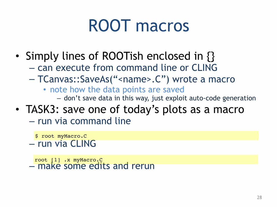
• Simply lines of ROOTish enclosed in {} – can execute from command line or CLING – TCanvas::SaveAs(“<name>.C”) wrote a macro
• note how the data points are saved – don’t save data in this way, just exploit auto-code generation
• TASK3: save one of today’s plots as a macro – run via command line
– run via CLING
– make some edits and rerun
$ root myMacro.C
root [1] .x myMacro.C
28
ROOT macros
• the { insert ROOTish here } macro format is only interpretable by CINT/CLING – compilation requires more conventional (but
not quite) C++ style coding – strictness dependent on choice of compiler • native ROOT compiler • (one of) your system(s) compiler(s)
– will return to macro compilation in week IV
29
Trees
• Histograms are useful, but they only store a single parameter – can extend to 2D hist of entries*weights with
bin errors, but still limited
• How to store information across many channels? – use TTrees! • n.b. there were no namespaces in C++ when ROOT
began, hence the T prefix on all ROOT types
30
Trees
• Trees in ROOT have branches and leaves – they also offer compression and I/O optimisation
• The branches can be basic data types or user defined classes – single instances of or multi-dimensional containers
of
• One usually saves data at the event level – so the Tree level data usually has structure
• many tracks and vertices in a single event – tracks and vertices have their own sub structure
31
Trees
• You can add branches (TBranch) and leaves (TLeaf) to (T)Trees by hand – but this is not the ROOT preferred method!
• though you will undoubtedly encounter it many times,
• The correct/expected way to read and write to a Tree is to use a class that encapsulates your data – then your Tree just contains a reference to this struct/
object • no need to reference all the individual parameters
• Writing classes to a Tree requires compilation – this is covered later
• for now just focus on reading data in a Tree
32
Trees
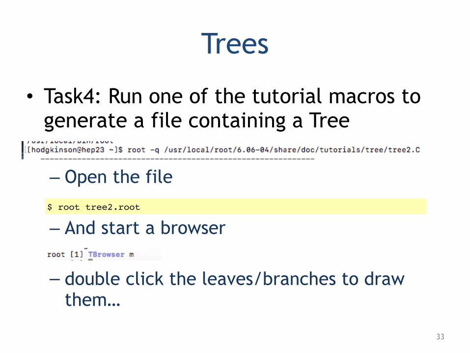
• Task4: Run one of the tutorial macros to generate a file containing a Tree
– Open the file
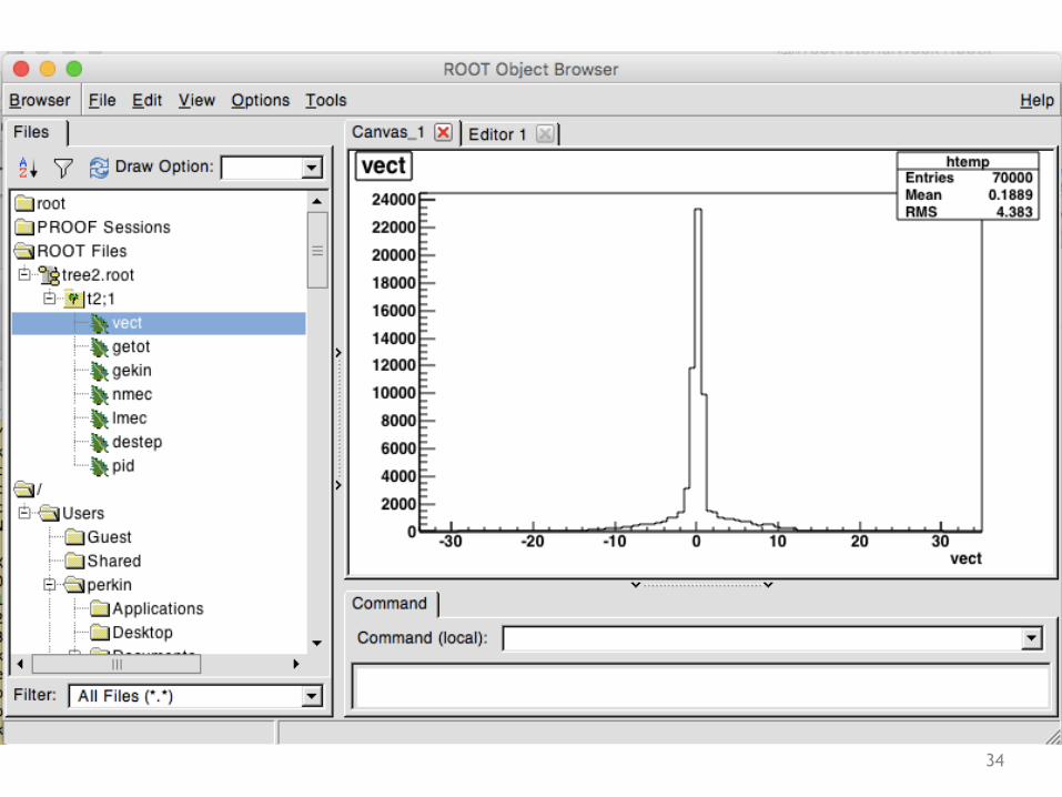
– And start a browser
– double click the leaves/branches to draw them…
$ root tree2.root
33
34
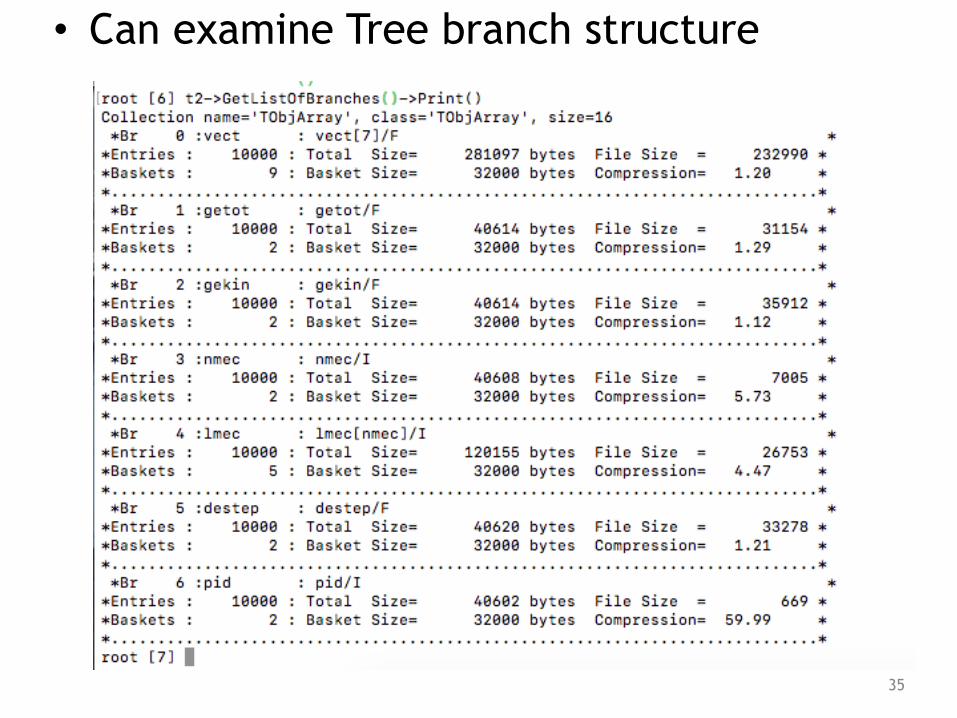
• Can examine Tree branch structure
35
Trees
• notice that pointer to Tree t2 is automatically instantiated – Tree was loaded into global directory when
file was opened • FUN TASK: start a new root session and type and
list the global file pointer, gFile->ls()
• looking at branches, can see some are arrays – can plot elements on different axesroot [4] t2->Draw("vect[0]:vect[1]:vect[2]”)
36
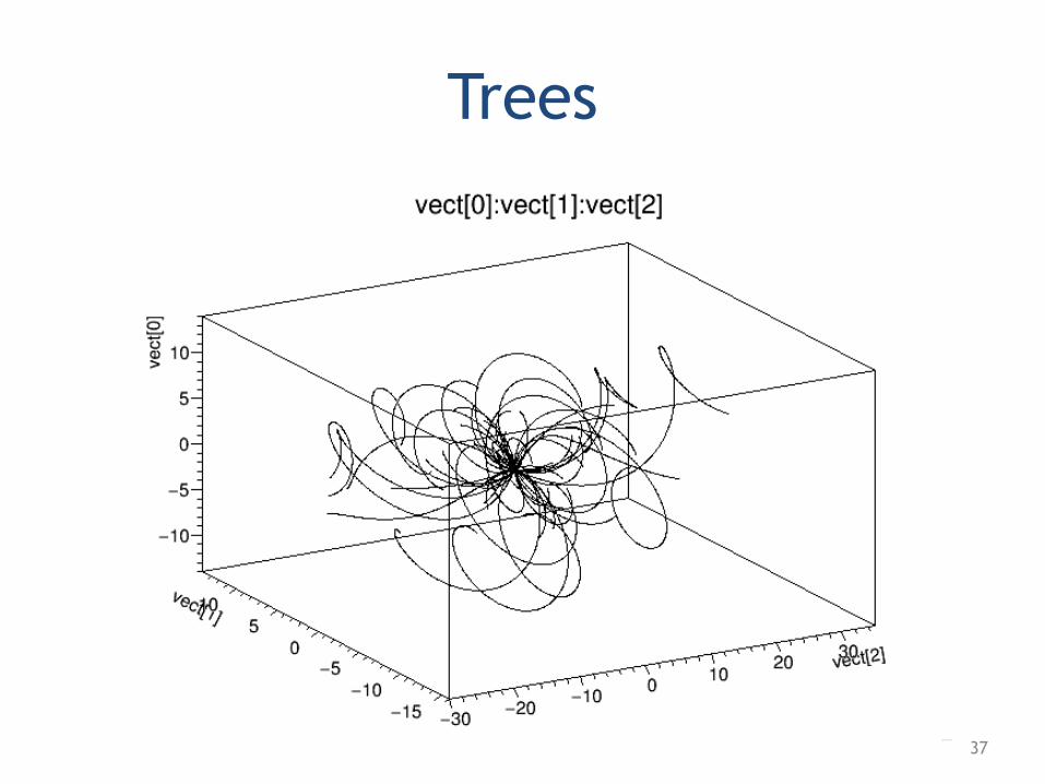
Trees
37
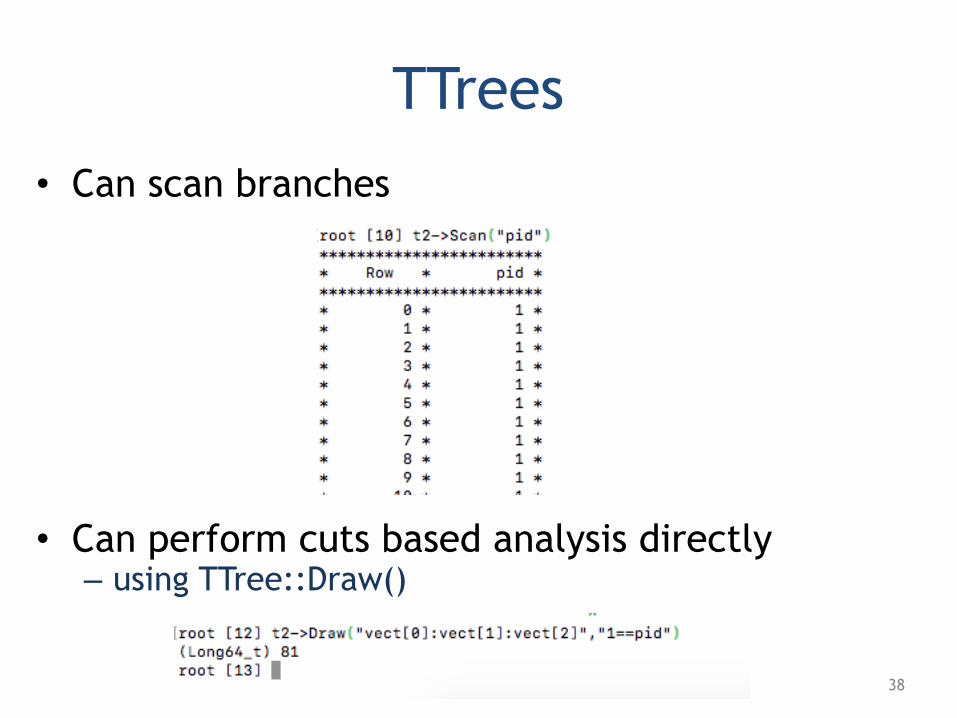
• Can scan branches
• Can perform cuts based analysis directly – using TTree::Draw()
TTrees
38
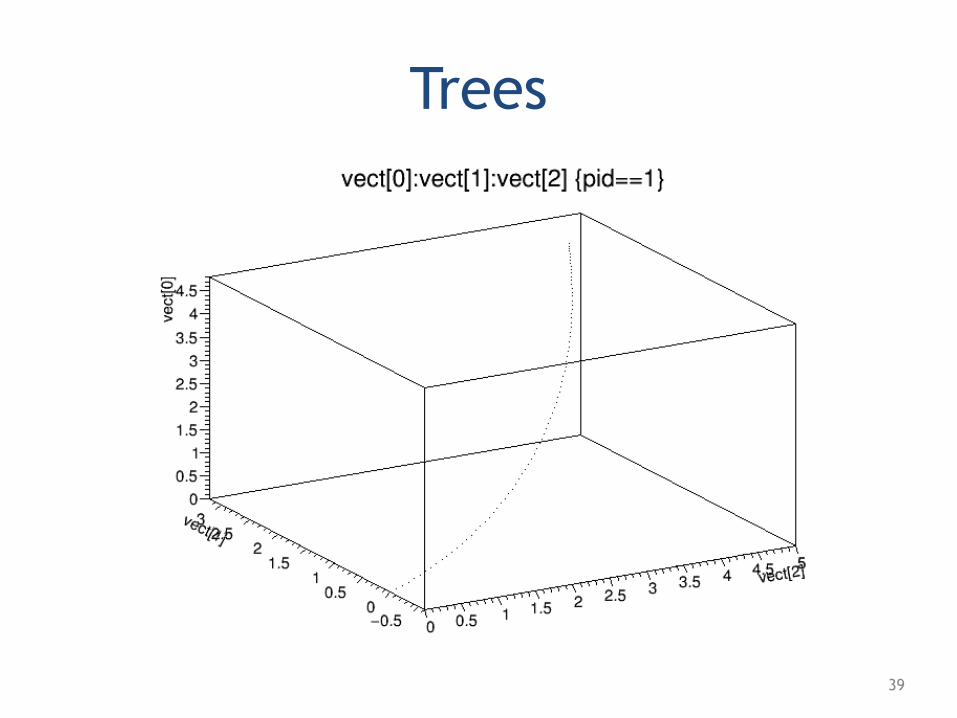
Trees
39
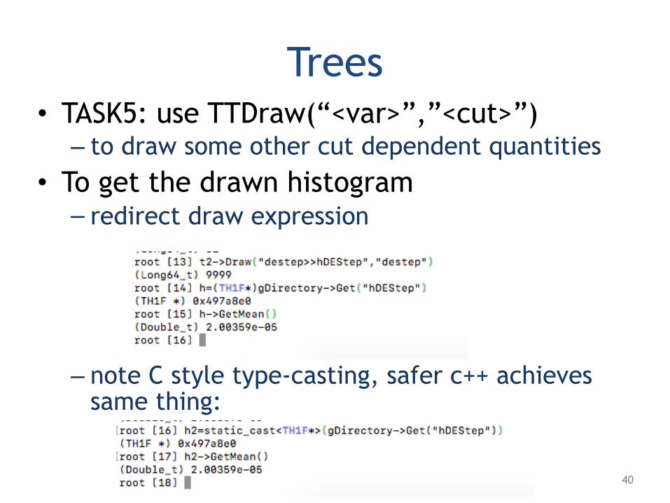
Trees• TASK5: use TTDraw(“<var>”,”<cut>”) – to draw some other cut dependent quantities
• To get the drawn histogram – redirect draw expression
– note C style type-casting, safer c++ achieves same thing:
40
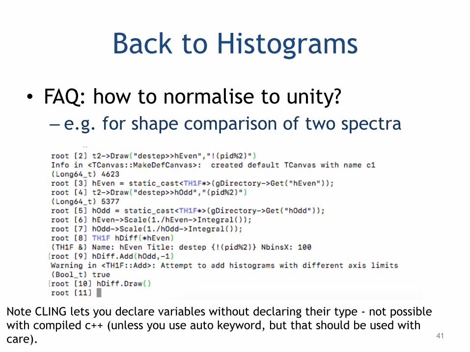
Back to Histograms
• FAQ: how to normalise to unity? – e.g. for shape comparison of two spectra
41
Note CLING lets you declare variables without declaring their type - not possible with compiled c++ (unless you use auto keyword, but that should be used with care).
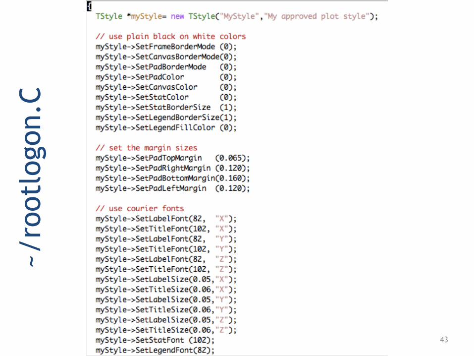
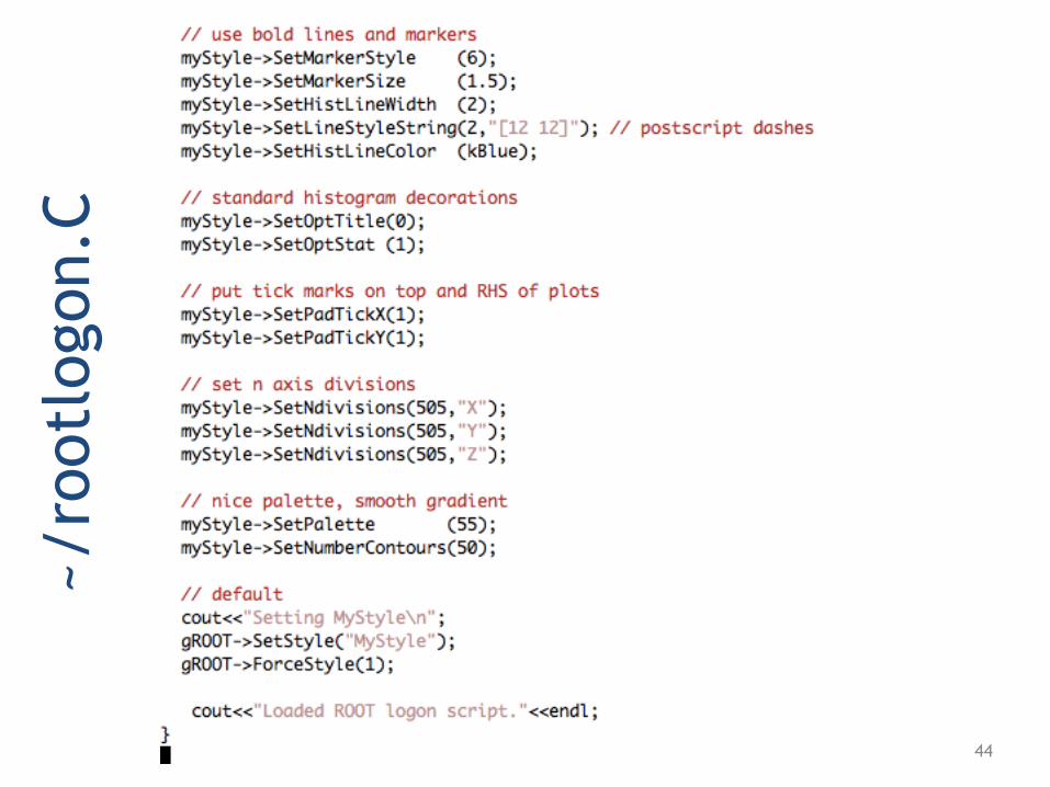
~/rootlogon.C
• you can place a macro in your home area that makes some useful definitions – e.g. stylistic changes
42
~/ro
otlo
gon.
C
43
~/ro
otlo
gon.
C
44
Closing remarks
• RTFM – there’s a lot of documentation out there
• likely someone has faced your issue already – also check the ROOT forum
• Have highlighted some ROOTisms today – there are many more to come
• remember not to assume what you see is good coding practice
• Next time: – I/O and memory – fitting and spectral analysis
• Any questions? • Also [email protected] for questions….
45