HEDGING HOUSING RISK IN

THE NEW ECONOMY: IS THERE

A CONNECTION, AND SHOULD

FIRMS CARE?

Nathan Berg, University of Texas at Dallas, USA

ABSTRACT

This paper analyzes housing price dynamics in and outside of TelecomCorridor, a region near Dallas, Texas, with a high concentration of neweconomy firms. Using separate home price indexes in and outside thisregion, the paper tests whether home values are more volatile in the neweconomy area and compares mean-variance efficient portfolio weights onhousing. The problem of hedging housing price volatility appears to bemore severe in the high tech sector, suggesting that new economy firmsmay benefit by offering workers various forms of home price insurance inlieu of cash wages.

I. INTRODUCTION

There is abundant evidence that imperfections in residential real es-tate markets burden homeowners with unwanted risk. These imperfectionsinclude housing market illiquidity, high transactions costs, predictabilityof housing market returns and, perhaps most important, the absence offinancial instruments with which to hedge against declines in home val-ues. Empirical evidence of housing market imperfections and theoreticaldiscussions of hedging instruments are discussed in Englund, Hwang andQuigley (2002), Flavin and Yamashita (2002), Clayton (2001), Case andShiller (1996, 1990).

This paper explores whether previously documented imperfections inhousing markets are more severe for stakeholders in the so-called “neweconomy,” i.e., for workers, owners, and property-owning neighbors near

firms with a high degree of co-investment in human and financial capital,or a high degree of real option characteristics. The central empirical ques-tion is whether housing markets in areas with high concentrations of neweconomy firms operate differently from housing markets in other locations.In the context of comparing new and old economy housing markets, a re-lated normative issue arises as to whether new economy firms and workersmight mutually benefit from experimenting with labor contracts that fea-ture a housing market option component. Gu and Kuo (2002), Iacovielloand Ortalo-Magne (2002), and Brown (2000) describe a variety of optioncontracts and other financial instruments designed for the purpose of hedg-ing home price risk.

The following is an overview of this paper. Section 2 discusses theoreti-cal reasons for suspecting that housing markets behave differently in areaswith high concentrations of new economy firms. Section 2 also introducesthe normative issue at stake — how to hedge housing risk, and whethernew economy firms are in a special position to innovate and possibly profitby providing home price insurance to workers. Section 3 introduces theempirical component of the analysis, drawing on a sample of more than300,000 home sales from Dallas County, 1979-2000, which includes a highlyconcentrated new economy sector, Telecom Corridor. A descriptive profileof that area, details on price index methodology, and a number of statisticaltests are presented. Section 4 uses return and volatility measures within astandard mean-variance portfolio framework to analyze and compare opti-mal weights on housing in new and old economy areas. Finally, Section 5attempts to link differences in the severity of the housing risk problem asrevealed by portfolio analysis to specific policy prospects for new economyfirms.

II. HOUSING MARKETS IN THE NEW ECONOMY

There are several reasons to suspect that residential housing marketswith concentrations of new economy workers might be more volatile thanhousing markets in other areas. More than other firms, new economy firmshave attempted to tie their employees’ earnings to the market value of thefirm. In so far as this shift has led to greater volatility in aggregate personalearnings through time, it seems likely that new economy workers’ demandfor housing, which theory suggests should depend on anticipated lifetimeearnings, would fluctuate more widely, too. Assuming that the market sup-ply curve for housing is positively sloped rather than flat, wider fluctuationsin the market demand curve would therefore cause wider variation in theprice of residential housing.

A second reason why geographic areas containing new economy firmsmight see unusually large fluctuations in housing prices stems from the im-portance of “flexibility” as a core managerial principle at such firms. Theflexibility principle when applied to decisions about hiring and lay-offs (orsimply manifest in a workplace culture that encourages workers to actively

seek new positions within the firm that entail geographic relocation), wouldseem to lead directly to shorter than average residential tenure and moreturnover in the housing market. High turnover, if it is lumpy in the sensethat surprise hiring and lay-off decisions are of large magnitude and concen-trated at certain points in time, implies greater volatility in housing pricereturns.1

Thus, the conjecture is that new economy human resources practicesmake old housing market problems worse.2 On the other hand, there isalso reason to hope that new economy firms may by well positioned to in-troduce innovative labor contracts with home price risk sharing featuresthat potentially improve the efficiency of housing markets. New economyfirms are highly invested in human capital. They have a proven trackrecord using options and innovative forms of non-cash employee compen-sation — these include greater work time flexibility (e.g., telecommuting,non-standard working hours, time off for elder car), tax friendly payrollservices (e.g., medical savings accounts and 401K retirement accounts),and upscale lifestyle amenities (e.g., onsite exercise trainers, masseuses andgourmet chefs). New economy firms also tend to be financially sophisti-cated, accustomed to using derivatives markets in dealing with risk.

The possibility that new economy firms will find it in their interest tooffer their employees risk sharing benefits associated with home ownershipfinds support in the following observations. First, workers at new economyfirms bear a portion of the housing market volatility that their employerscause. In equilibrium, workers will demand a wage premium to locate innew economy areas as compensation for bearing greater housing marketrisk. Seen in this light, additional housing market risk is an indirect costassociated with accomplishing other profit-enhancing objectives. Becausethe firm internalizes a portion of the volatility costs it imposes on its neigh-bors, it has an incentive to take action in moderating the costs of housingmarket risk. Creating new risk sharing opportunities for workers who wantto be homeowners can be viewed as part of the broader objective of cuttingcosts.

The question of whether cost-effective risk sharing mechanisms are ac-tually feasible depends on workers’ willingness to accept lower cash wagesin exchange for firm-administered home price insurance (workers’ degree ofrisk aversion), the tax treatment of firm-administered insurance, and thefirm’s ability to price housing risk and find mechanisms for hedging theadditional risk it assumes by writing labor contracts with home insuranceprovisions. In so far as new economy housing market volatility results in awage premium that new economy firms must pay, and to the extent thatnew economy firms have a greater propensity to innovate when it comesto human resources and non-cash compensation, then such firms must beconsidered among the leading candidates for improving housing market ef-ficiency. In particular, there may be scope for mutually beneficial employeebenefits packages that provide insurance against housing market risk while

reducing overall labor costs. This broader normative issue is discussed againin the Section 5 and motivates the empirical investigation that follows.3

III. THE NEW ECONOMY SECTOR OF DALLASCOUNTY

The data presented in this paper consist of all single-family home salesrecorded in the multiple listing service of Dallas County in the State ofTexas from 1979-2000. Dallas County is the heart of the 12-county Dal-las/Fort Worth Consolidated Metropolitan Area (CMSA) which has a laborforce of 2 million and a population of 5 million, making it the 9th largestCMSA in the U.S. The latest Census shows high rates of population growthin the area that outpace the national average. Population projections indi-cate that the area will be the 4th largest CMSA by 2010.

The “new economy” aspect of Dallas is substantial. The compositionof its business sector is heavily weighted toward technology-based services,high-tech manufacturing, retail and other services. Relatively little heavymanufacturing takes place in the area. The volume of economic activityin the Dallas area is large, both in absolute terms and in proportion toits population. According to the Greater Dallas Chamber of Commerce, ifthe Dallas CMSA were a country, its GDP would rank 24th in the world(http://www.gdc.org).

Although there are several “business parks” in the Dallas area, thelargest and most precisely defined (in terms of geographical boundaries andits emphasis on high-tech business enterprise) is Telecom Corridor. Tele-com Corridor is a “T”-shaped region comprised of two 10-mile vertical andhorizontal stretches centered on Richardson, Texas, a northern suburb ofthe City of Dallas, about 10 miles north of downtown. The high-tech orien-tation of the region to the north of Dallas owes in large part to the foundersof the Texas Instruments Corporation who located company headquartersthere in the 1960s. They also helped found a technology-based researchuniversity (now University of Texas at Dallas) and played an instrumentalrole in attracting telecommunications firms like MCI WorldCom and Nortelto the area.

In 1988, when the Fujitsu Corporation announced it would establisha 100 acre corporate campus in the area, the Dallas Morning News firstreferred to the area as “Telecom Corridor.” The Richardson Chamber ofCommerce eventually trademarked the phrase in 1992. Today, TelecomCorridor is home to over 600 high-tech companies and contains the largestconcentration of telecommunications firms in the U.S. Among these areHewlett Packard, Compaq, Nortel, Alcatel, and Cisco Systems.

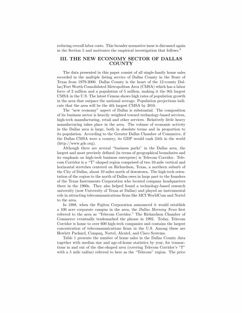
Table 1 presents the number of home sales in the Dallas County datatogether with median size and age-of-home statistics by year, for transac-tions in and out of the disc-shaped area (covering Telecom Corridor’s “T”with a 5 mile radius) referred to here as the “Telecom” region. The price

Year

Num

ber o

f

Sale

s

Media

n

Pric

e

Media

n

Square

Feet

Media

n

Age o

f

Dw

ellin

g

Num

ber o

f

Sale

s

Med

ian

Pric

e

Med

ian

Squ

are

Feet

Med

ian

Age o

f

Dw

ellin

g

1979

1,2

64

68,0

00

1,9

28

16,6

75

46,2

00

1,4

32

14

1980

2,1

97

78,5

00

1,8

77

58,6

64

54,3

37

1,4

20

18

1981

1,0

86

70,5

90

1,7

05

76,8

34

60,0

00

1,4

44

19

1982

1,6

83

98,5

00

2,0

22

74,5

78

65,0

00

1,4

80

13

1983

2,9

46

110,0

00

2,0

49

810,3

71

73

,500

1,5

03

18

1984

2,9

33

119,0

00

2,0

88

911,1

36

81

,317

1,5

47

19

1985

2,4

78

118,0

00

2,0

38

10

11,1

35

86

,000

1,5

56

20

1986

2,6

34

122,5

00

2,0

59

11

10,5

05

84

,499

1,5

40

17

1987

2,2

17

125,0

00

2,1

42

11

9,0

11

89

,000

1,6

57

15

1988

2,2

12

112,0

00

2,1

30

11

8,9

12

83

,500

1,6

51

15

1989

2,4

87

109,0

00

2,1

28

12

11,0

42

82

,000

1,6

64

13

1990

2,4

65

107,5

63

2,1

00

14

10,8

27

83

,000

1,6

71

17

1991

2,2

30

104,3

33

2,0

47

15

10,9

02

79

,000

1,6

49

18

1992

2,5

30

103,0

00

2,0

28

16

13,0

87

77

,500

1,6

30

19

1993

2,7

53

105,0

00

2,0

20

17

14,9

25

79

,000

1,6

30

20

1994

2,7

47

103,0

00

2,0

07

18

15,2

91

78

,900

1,6

14

22

1995

2,4

71

106,0

00

2,0

02

20

14,2

51

84

,000

1,6

62

23

1996

2,4

98

115,9

50

2,1

02

21

14,1

91

91

,896

1,7

17

24

1997

2,6

76

125,0

00

2,1

64

21

14,6

57

96

,500

1,7

25

24

1998

3,0

09

130,0

00

2,1

40

22

16,0

40

102

,000

1,7

26

24

1999

2,9

35

132,0

00

2,0

64

24

16,1

31

103

,000

1,6

74

26

2000

3,1

47

139,5

00

2,0

32

24

18,4

36

114

,500

1,7

03

22

All Y

ears

53,5

98

112,0

00

2,0

48

16

257,6

01

84,0

00

1,6

23

19

# P

ropertie

s

Table

1: N

um

ber o

f Sale

s, Media

n S

ize a

nd A

ge b

y Y

ear

Tele

com

Corrid

or A

rea

Non-T

ele

com

Co

rridor A

reas

34,2

94

175,0

95

data in Table 1 are unadjusted for inflation. Telecom area houses are no-ticeably larger (in terms of interior square feet, but not lot size), newer,and have higher prices. The total number of sales in the sample is 311,199.Because many of the homes in the sample are sold more than once in thetime interval 1979.1 through 2000.12, the number of unique dwellings inthe sample is considerable lower: 34,294 in the Telecom area and 175,095in the non-Telecom area. Although the sales data in Table 1 are broken outby year, the date of each sale is observed to the nearest month, making itpossible to construct monthly, quarterly, 6-month, or annual price indexesfrom which a representative “return on housing” can be computed.

Price Index MethodologyThe estimation of representative price series for the Telecom and the

non-Telecom areas, respectively, serves as a preliminary step toward com-puting expected real returns, covariance matrices (for housing returns andother assets such as stocks and bonds), and ultimately minimum-varianceportfolio weights. In spite of its intermediate status within the overall archi-tecture of that research agenda, the methodological challenges surroundingresidential real estate indexing are daunting and require extra attention.The technical issues that thwart aggregation of individual home sales intoa reasonable summary or spot price for real estate have in the past andcontinue to occupy the attention of leading real estate economists. En-glund, Quigley and Redfearn (1999), Zabel (1999), and Wang and Zorn(1997) contain discussions that provide an overview of home price indexmethodology and its outstanding problems.

Perhaps the biggest problem in choosing a summary statistic for homevalues has to do with disentangling changes in the quality of homes fromchanges in the market price for a representative house, holding qualityconstant. For example, if new homes in a particular area are twice as bigas existing homes, and the average price of a home increases as a result,it does not follow that owners of smaller homes can now sell their homesat a higher price. In other words, changes in the average sales price maybe a poor indicator of changes in the value of the average house. Newerhomes built with better technology, depreciation due to wear and tear, andimprovements to existing homes (or beneficial environmental change suchas the growth of attractive tree cover) are just some of the factors thatcreate problems for measuring housing market returns.

Techniques for computing a housing price index generally fall into oneof four categories: summary, repeat sales, hedonic and hybrid (Wang andZorn, 1997). Probably the most widely sited summary measures of homeprices in the aggregate are per-period mean and median prices. For ex-ample, the National Board of Realtors reports the median price of existinghome sales each month, and this statistic is widely cited in the news me-dia. Repeat sales indexes, on the other hand, measure change in homevalues by comparing sales prices for identical homes sold at different points

of time. The repeat sales technique attempts to control for difficult-to-measure changes in quality by limiting price comparisons to pairs of same-home sales prices arranged chronologically through time (see Shiller, 1991;Case and Quigley, 1987; and Bailey, Muth and Nourse, 1963, for details).Unlike the repeat sales technique, the hedonic method uses additional dataabout the characteristics of individual homes, such as number of bathrooms,square feet, proximity to good schools and other amenities. The strategyof the hedonic method is to explicitly control for variation in home featuresthat otherwise make it difficult to compare prices. Hybrid techniques com-bine repeat sale and hedonic price models in an attempt to use all availableinformation and more precisely estimate changes in aggregate home prices.

Fortunately, the Dallas data contain enough information to constructdifferent price indexes and compare their performance. From sales pricedata, monthly means and medians are straightforward to compute. Theproperties in the sample have unique id numbers from which same-housesales can be linked for the purpose of computing the repeat sale index. Thedata also include an abundance of housing characteristic controls, includingyear built, number of bathrooms, square feet, wet bars, appraisal value ofswimming pools and saunas, etc. In addition, the data are geo-coded andlinked to census tract data on tract-specific demographic information suchas median age, racial composition, the fraction of housing units that arerentals, and the average size of a household.

Table 2 presents mean values for some of the most important among thenumerous housing characteristic variables in the Dallas data. The averageTelecom-area home is bigger, newer, possesses more in-house amenities, andis located in a neighborhood that is whiter, younger, and more affluent.It is important to realize, however, that it is unclear based on Table 2whether a physically identical home located in a Census tract with identicaldemographic characteristics would be worth more in the Telecom or Non-Telecom area. In other words, the difference in average price in Table 2,by itself, provides no help in determining whether Telecom homes sell formore because they are in the Telecom area or because they happen to behomes with a greater quantity of amenities which would be valuable in anylocation.

Table 2 also presents means grouped according to whether a particu-lar property appears more than once in the sample. It is worthwhile tocompare so-called repeat sale homes to those involved in only a single sale.When considering the external validity with which changes in the repeat-sales price index may be used to make inferences about the population ofall home sales, paying attention to systematic differences between thosetwo categories is crucial. The average repeat sale home is larger and worthmore. The large sample sizes lead to very small root-N adjusted standarderrors, and many statistically significant differences among the four sub-groups broken out in Table 2.

mean

s.e.m

eans.e.

mean

s.e.m

eans.e.

mean

s.e.

Attrib

utes o

f Ind

ivid

ual D

wellin

gs

price

13

4,6

30

38

7.6

35

12

0,6

91

29

8.4

64

11

4,1

39

35

6.8

76

12

9,8

59

35

8.4

13

12

1,0

06

25

6.1

06

squ

are feet2

,15

3.2

83

.31

71

,81

0.1

01

.65

71

,80

5.5

12

.25

51

,91

7.3

42

.00

81

,86

9.2

01

.50

3

age o

f ho

use

17

.11

0.0

47

23

.10

0.0

35

22

.11

0.0

47

22

.04

0.0

41

22

.07

0.0

31

fireplaces

0.8

80

.00

20

.76

0.0

01

0.7

20

.00

10

.82

0.0

01

0.7

80

.00

1

full b

aths

2.2

50

.00

31

.92

0.0

01

1.9

10

.00

22

.02

0.0

02

2.1

00

.00

1

half b

aths

0.2

90

.00

20

.23

0.0

01

0.2

40

.00

10

.25

0.0

01

0.2

40

.00

1

wetb

ars0

.29

0.0

02

0.1

10

.00

10

.11

0.0

01

0.1

70

.00

10

.14

0.0

01

po

ol ap

praisal

2,7

76

.46

21

.41

21

,37

4.3

08

.11

11

,20

6.2

51

0.2

90

1,9

25

.36

11

.04

21

,61

5.8

17

.71

9

miles fro

m d

ow

nto

wn

11

.92

0.0

08

10

.46

0.0

08

10

.91

0.0

10

10

.57

0.0

09

10

.71

0.0

07

Teleco

m1

.00

0.0

00

0.0

00

.00

00

.19

0.0

01

0.1

50

.00

10

.17

0.0

01

Sin

gle S

ale Tran

saction

0.3

70

.00

20

.44

0.0

01

1.0

00

.00

00

.00

0.0

00

0.4

30

.00

1

Cen

sus T

ract Variab

les

percen

t black

0.0

90

.00

00

.15

0.0

00

0.1

60

.00

10

.12

0.0

00

0.1

40

.00

0

percen

t asian0

.09

0.0

00

0.0

40

.00

00

.04

0.0

00

0.0

50

.00

00

.05

0.0

00

percen

t hisp

anic

0.1

20

.00

00

.22

0.0

00

0.2

30

.00

10

.19

0.0

00

0.2

10

.00

0

percen

t 18

or u

nd

er0

.25

0.0

00

0.2

80

.00

00

.28

0.0

00

0.2

70

.00

00

.27

0.0

00

med

ian ag

e (tract residen

ts)3

6.7

80

.02

13

3.5

00

.01

33

3.2

40

.01

93

4.6

90

.01

43

4.0

70

.01

2

averag

e ho

useh

old

size2

.65

0.0

02

2.7

60

.00

12

.79

0.0

02

2.6

90

.00

12

.74

0.0

01

percen

t ow

ner o

ccup

ied0

.66

0.0

01

0.6

60

.00

00

.66

0.0

01

0.6

60

.00

00

.66

0.0

00

Nu

mb

er of S

ales

Variab

les

Tab

le 2: M

ean H

ou

sing

Ch

aracteristics and

Stan

dard

Erro

rs

Teleco

mN

on

-Teleco

mS

ing

le Sale

Tran

saction

s

Rep

eat Sale

Tran

saction

sA

ll Sales

31

1,1

99

No

te: a nu

mb

er of in

dep

end

ent v

ariables u

sed in

estimatin

g th

e hed

on

ic price in

dex

are no

t listed ab

ov

e. Th

ese inclu

de 1

64

(=22

x1

2)

mo

nth

-year tim

e du

mm

ies, du

mm

y v

ariables fo

r each o

f 14

scho

ol d

istricts located

in D

allas Co

un

ty (asid

e from

the D

allas Ind

epen

den

t

Sch

oo

l District), an

d u

p to

fou

rth-o

rder p

oly

no

mial tran

sform

s of tw

o v

ariables: ag

e of h

ou

se and

distan

ce from

do

wn

tow

n.

53

,59

82

57

,60

11

33

,96

71

77

,23

2

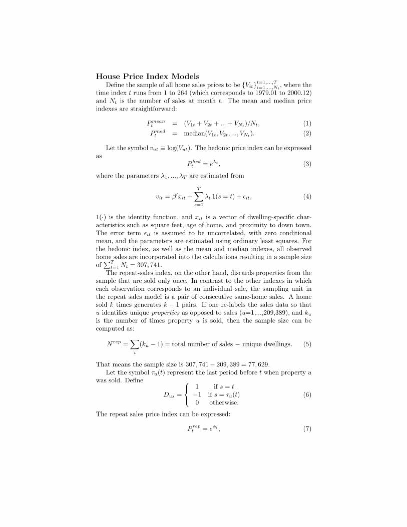
House Price Index ModelsDefine the sample of all home sales prices to be {Vit}t=1,...,T

i=1,...,Nt, where the

time index t runs from 1 to 264 (which corresponds to 1979.01 to 2000.12)and Nt is the number of sales at month t. The mean and median priceindexes are straightforward:

Pmeant = (V1t + V2t + ... + VNt)/Nt, (1)Pmed

t = median(V1t, V2t, ..., VNt). (2)

Let the symbol vut ≡ log(Vut). The hedonic price index can be expressedas

P hedt = eλt , (3)

where the parameters λ1, ..., λT are estimated from

vit = β′xit +T∑

s=1

λt 1(s = t) + εit, (4)

1(·) is the identity function, and xit is a vector of dwelling-specific char-acteristics such as square feet, age of home, and proximity to down town.The error term εit is assumed to be uncorrelated, with zero conditionalmean, and the parameters are estimated using ordinary least squares. Forthe hedonic index, as well as the mean and median indexes, all observedhome sales are incorporated into the calculations resulting in a sample sizeof

∑Tt=1 Nt = 307, 741.

The repeat-sales index, on the other hand, discards properties from thesample that are sold only once. In contrast to the other indexes in whicheach observation corresponds to an individual sale, the sampling unit inthe repeat sales model is a pair of consecutive same-home sales. A homesold k times generates k − 1 pairs. If one re-labels the sales data so thatu identifies unique properties as opposed to sales (u=1,...,209,389), and ku

is the number of times property u is sold, then the sample size can becomputed as:

N rep =∑

i

(ku − 1) = total number of sales − unique dwellings. (5)

That means the sample size is 307, 741− 209, 389 = 77, 629.Let the symbol τu(t) represent the last period before t when property u

was sold. Define

Dus =

1 if s = t−1 if s = τu(t)0 otherwise.

(6)

The repeat sales price index can be expressed:

P rept = eφt , (7)

where the parameters φ1, ..., φT are estimated from the equation

vut − vuτ(t) =T∑

s=1

φsDus + µut, (8)

with uncorrelated although heteroskedastic, zero conditional mean µit. Theparameters φs can be efficiently estimated using generalized least squares,utilizing information about the dependence of Eµ2

ut on t and τ . See Shiller(1991) or the appendix on “Weighted Repeat Sales Method” in Englund,Quigley and Redfearn (1999). Unlike the hedonic model, the repeat-priceindex requires only prices, dates of sale, and a way to link properties throughtime.

Figure 1 plots the four monthly price indexes for non-Telecom homesales in Dallas County. Figure 2 plots the indexes for sales in the Telecomarea. The two Figures are scaled identically to facilitate comparison oflevels and volatility. Comparing the two, price appreciation in the non-Telecom area appears to be greater than in the Telecom area. However,according to the hedonic index, price appreciation from 1979 through 2000is actually greater in the Telecom area, increasing by a factor of 2.5 ratherthan 2.4 in the non-Telecom area.

The four measures of aggregate price level are normalized so that allindexes equal 1 when t = 1, in the period 1970.01. The four indexes appearto track one another fairly well, although there are systematic differencesin their levels, which could be potentially important to risk/return analysesof the two respective markets. Correlation matrices among the four priceindexes (not presented here due to space considerations) show a high degreeof inter-relatedness, with correlations mostly in the 90% range and neverlower than 86% in the non-Telecom region. The price indexes in the Telecomarea, however, are less consistent, with correlations as low as 70%. In bothareas, the repeat sales index is noticeably less correlated than the otherthree measures.

In Figures 1 and 2, the mean and median price indexes give the highestestimate of price appreciation in the housing market, while the repeat salesindex gives the lowest. This would appear to be the logical result of the factthat the mean and median price indexes conflate improved aggregate qual-ity (e.g., bigger, better built homes featuring more amenities) with priceappreciation of a uniform-quality unit of housing. The fact that mediansales are consistently less than mean sales in Figure 1 reflects the influenceof several multi-million dollar home sales each period in older upscale areaslocated in the non-Telecom area. Explaining why the hedonic index showshigher aggregate price levels than the repeat sales index is less obvious. Thismay result from differences in the two subpopulations — single-sales versusrepeat-sales homes. In an encompassing hedonic regression in which repeatsale and non-repeat sale homes are allowed to have different parameters,the data soundly rejects the hypothesis that the models are the same, with

19

80

19

82

19

84

19

86

19

88

19

90

19

92

19

94

199

619

98

20

00

1

1.5 2

2.5 3

3.5

me

an

me

dia

n

he

do

nic

rep

ea

t sa

les

me

an

m

ed

ian

h

ed

on

ic

rep

ea

t sa

les

Figure 1: N

on-Telecom H

ousing Price Indexes, 1979-2000

19

80

19

82

19

84

19

86

19

88

19

90

19

92

19

94

199

61

998

20

00

1

1.5 2

2.5 3

3.5

mea

n

media

n

he

do

nic

rep

ea

t sa

les

me

an

m

ed

ian

h

ed

on

ic

rep

ea

t sa

les

Figure 2: Telecom

Housing P

rice Indexes, 1979-2000

a χ2(304) Wald test statistic of 4779.0. The technique of Oaxaca decom-position (originally applied to wage differentials in empirical labor studies(Oaxaca, 1973)) reveals that the gap in expected price between repeat andnon-repeat sale homes is 17% attributable to coefficients and 83% attribut-able to regressors. The estimate of 17% is statistically significant with aχ2(304) Wald test statistic of 504.1, meaning that both market differencesand, to a greater extent, different x values play a role in explaining thedifferent behavior of the repeat-sale price index.

An important feature of the hedonic index in both Figures is its relativesmoothness. Apparently, changes in the mix of houses sold from one monthto another (which are netted out in the hedonic index), rather than fluctu-ations in the market price for a standard-characteristic home, accounts formost of the month-to-month fluctuation in average and median home prices.This is consistent with previous findings, such as those in Case and Shiller(1987) comparing repeat sales and median indexes. In principle, changesin the mix of homes sold should not affect the repeat sale index either, andthe repeat sales index should appear as smooth as the hedonic index. Thisis precisely the case in Figure 1, but not in Figure 2.4 Discrepancies insample sizes between Telecom and non-Telecom areas, and between repeat-sale and other price indexes, should be kept in mind in interpreting Figures1 and 2. The average number of repeat sales occurring each month is 127in the Telecom area and 545 in the non-Telecom area. The correspondingaverage sample sizes for price indexes that do not exclude single-sale homesare 203 and 975.

The remainder of the empirical analysis in this paper addresses the ques-tion of whether Figures 1 and 2 reflect genuinely different price processesin the Telecom and non-Telecom areas, i.e., different enough to matter ina substantive way to potential homeowners considering whether to moveto one area or the other. In a statistical sense, the two areas are clearlydistinct. An unconditional t test of the hypothesis that log prices are equalhas magnitude 87.1; a Telecom area dummy variable in a single hedonicregression using the entire sample has a large and statistically significantcoefficient; and an equality of coefficients test from two separate hedonic re-gressions on the Telecom and non-Telecom samples leads to a χ2(304) Waldtest statistic of 2152.8. Further evidence that Telecom and non-Telecom ar-eas are statistically differentiated can be seen in the monthly percentagechanges in the (unconditional) average price series. Figure 3 presents thesemonthly changes, and Figure 4 shows the standard deviation of log pricesin both areas. The two figures, combined with a highly significant equalityof variance F(203,203) test statistic of 1.66 (corresponding to the percent-age change series), indicate greater unconditional volatility in the Telecomarea.5

Thus, every statistical test that was attempted rejects the hypothesisthat Telecom and non-Telecom price processes are identical. However, theissue of whether hedging opportunities in the two regions are substantively

different requires a further set of comparisons. Using inflation-adjustedpercentage changes in the different aggregate measures of house prices, thefollowing sections compare average real returns, volatility of returns, andthe correlations between returns on housing and other assets.

IV. RETURNS ON HOUSING AND OTHERASSETS

Defining “Returns on Housing”Having constructed four monthly housing price indexes, the next step is

to compute a corresponding real return series by taking monthly percentagechanges (not difference of logs) and subtracting the percentage change inthe monthly CPI-U for the U.S. By itself, this calculation of “returns onhousing” neglects potentially important costs and benefits associated withhome ownership. The rental or consumption value of residing on the prop-erty one owns is an important benefit. And the tax advantages of homeownership can be substantial (e.g., both mortgage interest payments andcapital gains from owner-occupied home sales generally receive favorabletax treatment in the U.S.). Homes also require periodic expenditures onmaintenance and, in most places in the U.S., create a tax liability for theirowners. The “return” on housing clearly depends on these annual flows ofcosts and benefits in addition to capital gains, i.e., price appreciation.

The problem is analogous to computing the time series of returns ona common stock. Given a price series, it is easy to compute capital gainsover any time horizon. But dividends must be added in somehow in orderto accurately state the return on one share. In the case of investing in ahome, one needs to add in the flow of net benefits apart from capital gainsto compute the investment’s return. The approach here follows Flavin andYamashita (2002).

The following three equations represent the rental value (or home divi-dend) Dt, the costs of maintenance COMt, and the annual return on hous-ing Rt for a homeowner with marginal income tax rate φ:

Dt = (i + d)Pt−1 + PropertyTaxt (9)COMt = dPt−1 + (1 − φ)PropertyTaxt (10)

Rt =Pt + Dt − COMt − Pt−1

Pt−1(11)

= Pt/Pt−1 + i + φPropertyTaxt/Pt−1 − 1. (12)

The symbol i is the short-term real interest rate (assumed in Flavin andYamashita (2002) to equal 5%); d is the physical rate of depreciation (borneequally by renters and owners). Flavin and Yamashita argue that the rentalvalue equation (9) derives from the zero profit condition facing landlords,and operationalize the system of equations by plugging in reasonable valuesfor the various parameters: i = .05, φ = .28 + .05 (federal plus state

marginal tax rates facing the average investor), and PropertyTaxt/Pt−1 =0.025. Just how “reasonable” these values are, however, is open to question.

In the case of Dallas County, the Flavin and Yamashita numbers requireadjustments for several reasons. For one thing, there is no state income taxin Texas, and high property tax rates are relatively high (as a result). Itshould be noted that the problem of dealing with taxes is relevant whencomputing the returns on other assets, too. Therefore consistent conven-tions for making adjustments for taxes are required if the results are to becompared meaningfully. For example, Flavin and Yamashita compare allasset returns on an after-tax basis. They apply the marginal income taxrate φ to interest income and stock dividends, and treat capital gains onstocks as if they were unrealized and therefore untaxed.

Because tax rates differ for different investors and change through time,it would be ideal to include detailed income and property tax data to moreaccurately quantify the symbols in the algebraic expression for housingmarket return. Absent this information, however, I adopted the follow-ing strategy. I simply tested a variety of assumptions about the value ofi + φ(PropertyTax)/P and tried to develop some understanding of the de-gree to which the ultimate results are sensitive to their manipulation. Byinspecting the real annual return on housing (Rt) equation above, it is ob-vious that different assumptions about i, φ and PropertyTax/P amountto changing the entire ‘percentage change in real price’ series by a con-stant. Fortunately changing the constant does not lead to any change inthe covariance matrices needed to compute efficient portfolios.

Unfortunately, however, different choices of values for that constantdirectly affect the expected return data which are critical inputs in theportfolio weight calculation. The portfolio weights reported in the next sec-tion are highly sensitive to a one percentage point change in this quantity.However, the relative weight on housing between Telecom and non-Telecomportfolios is consistent even when the levels of the weights change as a re-sult of changing i + (PropertyTax)/P. Of course, by choosing a highervalue of i + (PropertyTax)/P, the expected return on housing increases,and optimal portfolios shift to contain more housing. Because the correla-tion of housing returns and other assets is unchanged, however, minimum-variance portfolios in the Telecom versus non-Telecom areas broadly retaintheir relationship to one another. For example, if Telecom homeowners’portfolios contain half the housing in non-Telecom homeowners’ portfo-lios when i + (PropertyTax)/P = 0.06, then the same will hold wheni + (PropertyTax)/P = 0.07, even though both portfolios will containmore housing.

To keep the comparisons as straightforward as possible, my analysisis taken on a pre-tax basis. In other words, I make no adjustments fortaxes. I also lower i to .04 in order to reflect the lower real interest ratesexperienced in the U.S. in the 1990s. Flavin and Yamashita’s choice ofi = 0.05 strikes me as too high (although possibly appropriate for the

1968-1992 data they used). They describe i as a short-term interest rate.Conceptually, it represents the opportunity cost of tying up capital in ahome, together with the assumption that the next best alternative to homeownership is short term bonds earning 5%.6

Empirical Estimates of Return and RiskTable 3 presents average returns for housing (according to four dif-

ferent indexes) in the Telecom and non-Telecom areas, as well as stocks(S&P 500 index), bonds (10-year constant maturity Treasury rate), andthe Wilshire REIT (Real Estate Investment Trust) index.7 Average returnsat monthly, quarterly, 6-month and annual time horizons (adjusted to anannual basis) are presented, based on geometric summation of monthlypercentage changes. For example quarterly returns are constructed as(1 + rt)(1 + rt+1)(1 + rt+2) − 1, and then converted to an annual basisby multiplying times 4. Each time-horizon specific block in Table 2 con-tains three rows: the (arithmetic) average return, the standard deviationof the (time-horizon specific) return, and the standard deviation of theaverage return, which simply involves division by the square root of thenumber of non-overlapping time-horizons in the sample minus one. Be-cause the Wilshire REIT index begins in December 1982, all calculationsin the remainder of this paper are based on monthly returns series whichare truncated to begin on that date, leaving only 18 instead of 22 years ofdata.

Comparing the first and third rows of each time horizon block in Table3, one finds only a few statistically significant disagreements in expectedreturn among the four indexes within and between each of the two ge-ographical regions. The hedonic index has the smallest standard errors,formally demonstrating its smoothness which was apparent in Figures 1and 2. Another point worth mentioning is that annual returns are lessvolatile than monthly returns (times 12), a fact at odds with the randomwalk model. This suggests that more complex dynamics may underlie thehousing price process.

Table 4 produces statistics that are analogous to those in Table 3, butthis time under the assumption that each asset follows a univariate AR(1)process, where the time increment t variously represents one month, threemonths, six months, or 12 months. The expected return statistics repre-sent the arithmetic average of one-period ahead conditional expectations.Under the assumption that the error process is ergodic, the time average ap-proaches the unconditional expectation (which could have been estimateddirectly by plugging in estimates of α and ρ into α

1−ρ). Empirical values forthe standard errors are computed on the basis of squared forecasting errors,taken as the difference between each period’s conditional expectation andrealized value.

The monthly returns in Table 4 are significantly autocorrelated, withlarge negative autocorrelation coefficients (“rho” in Table 4). Reverting

Mean

Median

Hedonic

Repeat-

SaleM

eanM

edianHedonic

Repeat-

Sale

S&P

500

10-year

T BillREIT

Monthly, T=217

Er x 120.068

0.0740.040

0.1020.077

0.0520.038

0.0410.105

0.0400.076

sigma_r x 12

0.8921.082

0.2571.455

0.8410.509

0.2160.333

0.5150.028

0.433

sigma_r x 12/(T-1)^0.5

0.0610.074

0.0170.099

0.0570.035

0.0150.023

0.0350.002

0.029

Quarterly, T=72

Er x 40.048

0.0490.040

0.0630.062

0.0470.037

0.0380.104

0.0400.075

sigma_[(1+r_t)(1+r_{t+1})(1+r_{t+2})] x 4

0.3550.391

0.1210.620

0.3370.208

0.1230.149

0.2960.022

0.277

sigma_[…

]/(T-1)^0.50.042

0.0460.014

0.0740.040

0.0250.015

0.0180.035

0.0030.033

6-month, T=36

Er x 20.041

0.0440.040

0.0360.060

0.0470.037

0.0380.103

0.0410.077

sigma_[(1+r_t)...(1+r_{t+5})] x 2

0.1950.243

0.0750.281

0.2110.143

0.0730.099

0.1910.018

0.211

sigma_[…

]/(T-1)^0.50.033

0.0410.013

0.0480.036

0.0240.012

0.0170.032

0.0030.036

Annual, T=18

Er0.037

0.0350.040

0.0260.053

0.0470.038

0.0390.105

0.0410.081

sigma_[(1+r_t)...(1+r_{t+11})]

0.1020.107

0.0540.138

0.0900.092

0.0620.091

0.1360.017

0.169

sigma_[…

]/(T-1\)^0.50.025

0.0260.013

0.0340.022

0.0220.015

0.0220.033

0.0040.041

Table 3: Random W

alk Model --- Arithm

etic Mean Real Returns on Housing and Other Assets

TelecomNon-Telecom

Other Assets

Mean

Med

ianH

edonic

Rep

eat-

Sale

Mean

Med

ianH

edonic

Rep

eat-

Sale

S&

P

500

10-y

ear

Bond

RE

IT

Month

ly R

eturn

s x 1

2 fo

r the "t =

1 M

onth

" AR

(1) M

odel, T

=217

E_t r_

{t+1} x

12

0.0

32

0.0

40

0.0

25

0.0

52

0.0

49

0.0

34

0.0

33

0.0

30

0.1

03

0.0

58

0.0

82

sigm

a_t(r_

{t+1}) x

12

0.7

88

0.9

95

0.2

44

1.2

75

0.7

84

0.4

81

0.2

15

0.3

25

0.5

13

0.0

30

0.4

25

sigm

a / (T-1

)^0.5

0.0

54

0.0

68

0.0

17

0.0

87

0.0

53

0.0

33

0.0

15

0.0

22

0.0

35

0.0

02

0.0

29

rho in

Month

ly A

R(1

)-0

.474

-0.4

03

-0.3

28

-0.4

89

-0.3

73

-0.3

45

-0.0

56

-0.2

14

-0.0

53

0.4

48

0.1

63

t stat for rh

o-7

.928

-6.4

96

-5.1

10

-8.2

48

-5.9

25

-5.4

19

-0.8

20

-3.2

24

-0.7

89

7.3

79

2.4

33

Quarterly

Retu

rns x

4 fo

r the "t=

1 Q

uarter" A

R(1

) Model, T

=72

E_t r_

{t+1} x

40.0

26

0.0

28

0.0

31

0.0

32

0.0

46

0.0

36

0.0

31

0.0

36

0.0

93

0.0

49

0.0

71

sigm

a_t(r_

{t+1}) x

40.3

11

0.3

60

0.1

17

0.5

09

0.3

22

0.2

03

0.1

21

0.1

48

0.2

94

0.0

23

0.2

75

sigm

a / (T-1

)^0.5

0.0

37

0.0

43

0.0

14

0.0

60

0.0

38

0.0

24

0.0

14

0.0

18

0.0

35

0.0

03

0.0

33

rho in

Quarterly

AR

(1)

-0.4

89

-0.3

90

-0.1

81

-0.5

69

-0.2

90

-0.1

90

-0.1

32

-0.0

53

-0.0

77

0.2

32

0.0

00

t stat for rh

o-4

.756

-3.5

99

-1.5

63

-5.8

67

-2.5

68

-1.6

43

-1.1

33

-0.4

50

-0.6

51

2.0

25

0.0

03

6-M

onth

Retu

rns x

2 fo

r the "t =

6 M

onth

s" AR

(1) M

odel, T

=36

E_t r_

{t+1} x

20.0

15

0.0

13

0.0

32

0.0

21

0.0

17

0.0

27

0.0

45

0.0

50

0.0

85

0.0

61

0.0

59

sigm

a_t(r_

{t+1}) x

20.1

56

0.1

90

0.0

72

0.2

40

0.1

59

0.1

31

0.0

70

0.0

95

0.1

86

0.0

26

0.1

98

sigm

a / (T-1

)^0.5

0.0

26

0.0

32

0.0

12

0.0

41

0.0

27

0.0

22

0.0

12

0.0

16

0.0

31

0.0

04

0.0

33

rho in

Six

-Month

AR

(1)

-0.6

04

-0.6

17

-0.1

10

-0.5

18

-0.6

37

-0.3

60

0.2

69

0.3

16

-0.1

13

0.5

21

-0.0

91

t stat for rh

o-4

.549

-4.7

10

-0.6

64

-3.6

35

-4.9

62

-2.3

15

1.6

76

1.9

97

-0.6

84

3.6

64

-0.5

49

Annual R

eturn

s for th

e "t = 1

Year" A

R(1

) Model, T

=18

E_t r_

{t+1}

0.0

35

0.0

24

0.0

66

0.0

09

0.0

52

0.0

32

0.0

56

0.0

38

0.0

81

0.0

61

0.0

64

sigm

a_t(r_

{t+1})

0.0

98

0.0

98

0.0

46

0.1

25

0.0

81

0.0

80

0.0

50

0.0

88

0.1

35

0.0

25

0.1

60

sigm

a / (T-1

)^0.5

0.0

24

0.0

24

0.0

11

0.0

30

0.0

20

0.0

19

0.0

12

0.0

21

0.0

33

0.0

06

0.0

39

rho in

Annual A

R(1

)0.1

16

-0.0

32

0.7

61

-0.3

96

0.1

62

-0.1

06

0.6

57

0.0

98

-0.2

09

0.5

93

-0.0

61

t stat for rh

o0.4

95

-0.1

38

4.9

75

-1.8

30

0.6

98

-0.4

53

3.7

00

0.4

16

-0.9

07

3.1

24

-0.2

59

Teleco

mN

on-T

elecom

Oth

er Assets

Tab

le 4: A

R(1

) Model --- A

verag

e Expected

Real R

eturn

s Usin

g A

R(1

) Models o

n H

ousin

g an

d O

ther A

ssets

behavior is especially severe in the Telecom area. The importance of au-tocorrelation, however, seems to dissipate with longer time horizons, andthe sign of many of the housing index autocorrelation coefficients switchesfrom negative to positive. Expected returns in Table 4 based on the AR(1)model are in general lower, and reveal sharper differences among the dif-ferent housing indexes than in the random walk model.

How Different Are Telecom and Non-Telecom Regions?By the two standard deviation criterion, very few significant differences

between expected returns in the Telecom and non-Telecom areas can beseen in Tables 3 and 4. The data easily reject formal (Wald) tests of thehypothesis that parameter values across the two samples are equal. Hous-ing market volatility as measured by standard deviation appears slightlygreater in the Telecom area, which would confirm one of the main hypothe-ses proposed in the introduction. However, without consulting a formalmeasure of precision for the estimated standard deviation, Tables 3 and4 by themselves do not add much weight to the claim that new economyhousing markets are distinctly risky. Although there is ample statistical ev-idence to differentiate the two regions, whether those differences translateinto something substantively important for homeowners in new economyareas is another question.

The outlined diagonals in Table 5 contain the same-index correlationsfor the Telecom and non-Telecom areas. By all measures, monthly returnsin the two areas are weakly correlated, never reaching more than 38%.Annual or 12-month returns are more correlated, but not uniformly: therepeat sale price indexes in the two areas in the random walk model, forexample, have 0% correlation. Comparing the degree to which home pricesare correlated with stocks, bonds, and REITs in the two areas, one findseveral large magnitude and opposite-sign disagreements.

Overall, Tables 3, 4 and 5 paint a pessimistic picture with respect to thegoal of estimating risk and return for investments in the housing market.Different investment horizons and different assumptions about the returnsprocess lead to significantly different quantifications of risk and return.Nevertheless, those differences are finite, and we can proceed by discussinga representative case and analyzing the sensitivities to changes in index,time horizon, and error structure.

How Much Housing Belongs in Minimum-Variance Port-folios?

This section computes the share of wealth allocated to housing in aminimum-variance portfolio. It is well known that the equivalent goals ofminimizing variance subject to a target level of expected return, and ofmaximizing expected return subject to a target level of variance, togetherwith normality assumptions, correspond to preferences represented by theconstant absolute risk aversion expected utility function. Table 6 containsminimum-variance portfolio weights (on housing, stocks, bonds and REITs)

Mean Median Hedonic

Repeat-

Sale Mean Median Hedonic

Repeat-

Sale

S&P

500

10-year

T Bill REIT

One-Month Returns Monthly Random Walk Model

Telecom Mean 1.00

Median 0.72 1.00

Hedonic 0.37 0.41 1.00

Repeat-Sale 0.14 0.01 0.26 1.00

Non-Tele. Mean 0.17 0.07 0.15 0.07 1.00

Median 0.18 0.14 0.19 -0.01 0.50 1.00

Hedonic 0.16 0.14 0.37 0.16 0.25 0.45 1.00

Repeat-Sale 0.13 0.16 0.18 0.10 0.10 0.19 0.29 1.00

Other S&P 500 0.02 0.06 0.10 -0.02 0.15 0.01 -0.03 -0.07 1.00

10-year T Bill -0.04 -0.02 0.10 0.07 -0.05 0.04 0.08 0.04 0.12 1.00

REIT 0.06 0.01 0.03 -0.05 0.01 0.06 -0.06 -0.09 0.10 0.08 1.00

12-month Returns Using Monthly Random Walk Model

Telecom Mean 1.00

Median 0.66 1.00

Hedonic 0.56 0.63 1.00

Repeat-Sale 0.00 0.18 0.42 1.00

Non-Tele. Mean 0.52 0.43 0.65 0.26 1.00

Median 0.68 0.65 0.61 -0.02 0.75 1.00

Hedonic 0.46 0.41 0.84 0.51 0.75 0.50 1.00

Repeat-Sale 0.56 0.58 0.74 0.04 0.70 0.78 0.71 1.00

Other S&P 500 0.03 0.13 0.11 0.60 0.23 -0.07 0.38 0.02 1.00

10-year T Bill 0.03 0.17 0.19 0.11 0.36 0.16 0.20 0.07 0.20 1.00

REIT 0.39 0.50 0.20 -0.18 0.30 0.30 0.25 0.21 0.23 0.41 1.00

"t = 1 Month" AR(1) Model

Telecom Mean 1.00

Median 0.72 1.00

Hedonic 0.41 0.44 1.00

Repeat-Sale 0.10 0.01 0.22 1.00

Non-Tele. Mean 0.21 0.14 0.19 0.02 1.00

Median 0.27 0.21 0.24 0.01 0.54 1.00

Hedonic 0.21 0.15 0.38 0.21 0.35 0.51 1.00

Repeat-Sale 0.16 0.20 0.23 0.14 0.15 0.24 0.32 1.00

Other S&P 500 0.04 0.05 0.12 -0.02 0.13 0.03 -0.02 -0.09 1.00

10-year T Bill 0.02 -0.05 0.16 0.20 -0.07 -0.02 0.09 0.06 0.08 1.00

REIT 0.07 0.01 0.07 -0.03 0.01 0.03 -0.07 -0.14 0.12 0.03 1.00 "t = 1 Year" AR(1) Model

Telecom Mean 1.00

Median 0.62 1.00

Hedonic 0.22 0.42 1.00

Repeat-Sale 0.19 0.26 0.55 1.00

Non-Tele. Mean 0.43 0.31 0.15 0.28 1.00

Median 0.65 0.56 0.19 0.07 0.70 1.00

Hedonic 0.25 0.12 0.42 0.47 0.58 0.22 1.00

Repeat-Sale 0.52 0.55 0.49 0.12 0.64 0.79 0.49 1.00

Other S&P 500 0.02 0.12 0.10 0.60 0.27 -0.03 0.46 0.00 1.00

10-year T Bill 0.02 0.12 0.14 0.11 0.11 -0.07 0.04 0.05 0.18 1.00

REIT 0.25 0.43 -0.20 -0.20 0.19 0.21 0.05 0.16 0.21 0.51 1.00

Other

Table 5: The Correlation of Real Returns

Telecom Non-Telecom

Targ

et

Retu

rnH

ousin

gS

tock

sB

onds

RE

ITS

Housin

gS

tock

sB

onds

RE

ITS

Month

ly R

andom

Walk

Model

0.0

00

0.0

86

-0.4

43

1.6

71

-0.3

14

0.0

02

-0.4

42

1.7

55

-0.3

15

0.0

84

0.0

10

-0.1

70

0.8

83

-0.3

45

0.6

32

0.0

15

0.8

81

-0.5

31

0.6

36

-0.1

85

0.0

20

-0.4

27

2.2

09

-2.3

60

1.5

78

0.0

27

2.2

04

-2.8

17

1.5

87

-0.4

54

0.0

30

-0.6

84

3.5

35

-4.3

76

2.5

25

0.0

40

3.5

26

-5.1

04

2.5

38

-0.7

23

0.0

40

-0.9

40

4.8

60

-6.3

91

3.4

71

0.0

52

4.8

49

-7.3

90

3.4

89

-0.9

92

0.0

50

-1.1

97

6.1

86

-8.4

06

4.4

17

0.0

64

6.1

72

-9.6

76

4.4

40

-1.2

61

0.0

60

-1.4

53

7.5

12

-10.4

22

5.3

63

0.0

77

7.4

94

-11.9

62

5.3

91

-1.5

30

0.0

70

-1.7

10

8.8

38

-12.4

37

6.3

09

0.0

89

8.8

17

-14.2

48

6.3

42

-1.7

99

0.0

80

-1.9

67

10.1

63

-14.4

52

7.2

56

0.1

01

10.1

40

-16.5

34

7.2

93

-2.0

68

0.0

90

-2.2

23

11.4

89

-16.4

68

8.2

02

0.1

14

11.4

62

-18.8

20

8.2

44

-2.3

37

0.1

00

-2.4

80

12.8

15

-18.4

83

9.1

48

0.1

26

12.7

85

-21.1

06

9.1

95

-2.6

06

0.1

20

-2.9

93

15.4

66

-22.5

14

11.0

40

0.1

51

15.4

30

-25.6

78

11.0

97

-3.1

44

0.1

40

-3.5

06

18.1

18

-26.5

45

12.9

33

0.1

76

18.0

76

-30.2

51

12.9

99

-3.6

82

0.1

60

-4.0

19

20.7

69

-30.5

75

14.8

25

0.2

01

20.7

21

-34.8

23

14.9

01

-4.2

20

0.1

80

-4.5

32

23.4

21

-34.6

06

16.7

18

0.2

25

23.3

66

-39.3

95

16.8

04

-4.7

58

0.2

00

-5.0

46

26.0

72

-38.6

37

18.6

10

0.2

50

26.0

12

-43.9

67

18.7

06

-5.2

96

0.3

00

-7.6

12

39.3

30

-58.7

90

28.0

72

0.3

74

39.2

38

-66.8

28

28.2

16

-7.9

86

0.4

00

-10.1

78

52.5

88

-78.9

44

37.5

34

0.4

98

52.4

65

-89.6

89

37.7

27

-10.6

76

0.5

00

-12.7

44

65.8

45

-99.0

98

46.9

96

0.6

22

65.6

91

-112.5

50

47.2

37

-13.3

65

Teleco

m C

orrid

or A

reaN

on-T

elecom

Corrid

or A

reasT

elecom

- Non-

Teleco

m

Weig

ht

Tab

le 6: O

ptim

al Portfo

lio W

eights --- T

elecom

Versu

s Non-T

elecom

Hom

eow

ners

for a range of levels of target expected return. The expected return andcovariance matrix come from the hedonic index and the monthly randomwalk model. After examining similar tables for other indexes, time horizonsand error structures, the weights in Table 6 are representative in at leasttwo senses. The optimal weight on housing is usually quite different in theTelecom area than in the non-Telecom area. When assumptions are changedthat elevate the expected return of housing, both areas’ housing weightsshift toward housing, but the relative differences persist. For example,given a particular covariance matrix, if Telecom portfolios start out withless housing in them, then even after housing becomes more attractive interms of expected return, Telecom portfolios remain comparatively shorton housing.

Table 6 shows that efficient portfolios over reasonable ranges of expectedreturn contain negative amounts of housing.8 The hedonic index, whichtypically is the least volatile among the housing indexes, and frequentlyhas one of the highest returns, is a good basis for comparison because itis, for the most part, the most favorable among the indexes for housing.Even under favorable circumstances (relatively low risk and high return)for housing investment, the wise homeowner (in a frictionless world withcomplete markets in risk) will not hold positive quantities net investment inhousing. The last column shows the difference between optimal weights onhousing for the two areas, demonstrating that Telecom homeowners shouldhold much less housing than non-Telecom homeowners. One may proposethe following generalization: the housing-risk hedging problem is more se-vere for new economy workers, because their optimal portfolio decisions ina world without constraints imposed by market imperfections contain farless housing than those of homeowners in traditional real estate markets.

V. Discussion and Conclusions

The housing market in Telecom Corridor, one of Dallas County’s great-est concentrations of new economy firms, has “new economy” features ofits own. Telecom Corridor homes earn an investment return that is morevolatile and more correlated with common stocks than housing returns inother areas. The correlation between Telecom and non-Telecom housingreturns is weak. For most model specifications and expected-return tar-gets, the optimal weight on housing (in a mean-variance efficient portfolio)is negative, and Telecom area portfolios generally contain less (more neg-ative) weight on housing than in other areas. Even when this is not thecase, efficient portfolios across the two areas are quite different.

According to the portfolio model, home ownership requires new econ-omy homeowners to mover farther away from their optimal behavior underperfect market conditions than is the case for homeowners in other areas.This implies that workers at new economy firms may be among the mosthighly motivated to adopt new hedging instruments provided by their em-

ployers. In other words, new economy workers may be willing to pay morefor contracts that insure against house price declines.

Unfortunately, existing classes of assets do not offer feasible hedging op-portunities for homeowners. The evidence is mixed as to whether the city-or region-wide price indexes presented in this paper could be used as effec-tive tools for hedging. One way to quantify the hedging value of a singleprice index is to regress individual home sale returns (using the repeat-salesample) on a constant and the “market return” given by the price indexover a corresponding time horizon. Following the textbook approach, re-turn volatility can then be decomposed into systematic and idiosyncraticcomponents (Shiller and Weiss, 2000; Case and Shiller, 1989). If moresophisticated housing future contracts incorporating the hedonic approachwere made available, then it might be possible to hedge a greater fraction ofhome price volatility by exploiting additional information about the char-acteristics of individual homes. In that case, the idiosyncratic componentwould be smaller and the error term in the hedonic regression, or 1 − R2,would provide an estimate.

If demand for insurance is strong in new economy areas, as the argu-ment above suggests, it is reasonable to hypothesize that risk-neutral neweconomy firms could profit by offering labor contracts which include someform of home price insurance and an offsetting reduction in cash wages.For example, a firm might consider writing a put option that has fair mar-ket value of $20, 000 (a valuation possibly provided by the firm’s lenderswho will be keen to monitor the balance sheet effects of any housing op-tion activity).9 The firm then offers its employees the option of switchingto a labor contract that delivers possession of the put to the employee inexchange for accepting $25, 000 less in cash compensation over a periodof several years. The firm receives 20% more for the put than its fair orrisk-neutral valuation. And sufficiently risk averse employees will be madebetter off.

The trade-off between cash wages and put option insurance is not zerosum, because a worker’s risk aversion leads to a willingness to pay functionthat is nonlinear in risk. Modeling this in detail is left for future study.Current tax rules may provide additional support for the idea that firmsare the logical institution to offer home price insurance. Because of lenientand ambiguous accounting rules concerning option contracts as employeecompensation, it may be possible that workers “pay” for employer providedinsurance with pre-tax dollars. This would make the proposals discussedabove even more attractive and encourage risk averse employees to over-come any hesitation in participating in a novel compensation plan.

Of course, writing put options on homes levers the firm with increaseddownside risk in the event that their own misfortune coincides with declin-ing home values in their vicinity. However, the firm stands to gain never-theless, because workers who are more risk averse than the firm, and whoenjoy additional tax benefits by reducing their cash compensation, will pay

more than the firm’s valuation of home puts in terms of reduced cash wages.Providing that workers who are holders of home put options enjoy prece-dence over other debtors in the event of default, the risk pricing expertise ofbanks and other investors would come into play. In fact, one way to pricehousing risk would be to approach a firm’s creditors with the wage plandescribed above and ascertain how their borrowing costs would rise as aresult of taking on an additional unit of employee-housing liability. Futurework in this direction should attempt to embed home insurance risk into atwo-sided economic model of workers and firms, derive a home put pricingformula, and explore the possible tax advantages to workers and firms whoexchange home price insurance for labor.

ENDNOTES

* Special thanks to James Murdoch for detailed advice in analyzing Dal-las County housing market data and to Richard Huckaba and KeithHeckathorn for their valuable input. Financial support from the Na-tional Academy of Science’s Urban Scholars Fellowship and the De-partment of Housing and Urban Development is gratefully acknowl-edged. Irene Ndugi and Kalpana Pai provided research assistance.An anonymous referee contributed significantly to the methodologyand presentation of this paper for which I am grateful.

Berg: Cecil and Ida Green Assistant Professor of Economics,University of Texas at Dallas, GR 31 211300, Box 830688, Richardson,Texas 75083-0688. Phone 1-972-883-2088, Fax 1-972-883-2735, Emailnberg@utdallas.edu

1. Pyhrr, Roulac and Brown (1999) review a large body of empiricalstudies that demonstrate evidence of cyclicity in real estate markets.

2. This paper assumes throughout that homeowners are better off, ce-teris paribus, the less exposed to housing market volatility they are.In contrast, Nordvik’s (2001) life-cycle model demonstrates that homeprices can be increasing in risk even in a market populated by risk-averse homeowners. This possibility greatly complicates the welfareanalysis of risk in housing markets and is not considered further inthis analysis.

3. There has been substantial commercial and academic interest in thedevelopment of new institutions for helping homeowners convert illiq-uid and risky home equity to other uses and/or reduce exposure toreal estate risk (Shiller and Weiss, 2000, 1999; Caplin, Chan, Free-man and Tracy, 1997; Sheffrin and Turner, 2001). The novel aspectof the normative discussion in this paper is its focus on the exchangeof housing risk by employers and employees.

4. Clapp and Giacotto (2002) compare repeat sale and hedonic indexesby different measures of forecasting efficiency, finding that the hedonicindex is the more efficient of two.

5. Measures of volatility in a panel data set such as this are somewhatsensitive to specification. For example, the Telecom area sample hasmany more observations in later years, whereas the non-Telecom sam-ple is more evenly balanced. Being more uniformly spread throughtime makes the non-Telecom prices have greater dispersion by somemeasures. Another problem is that same-period price dispersion canreflect a housing market with a greater variety of homes rather thangreater price volatility associated with individual homes of a partic-ular quality level. Another possibility left here to future research istime-varying volatility, i.e., the use of GARCH of stochastic volatilitymodels, in the analysis of housing market risk. Yet another approachis that of He and Winder (1999) who analyze cointegrating relation-ships and apply Granger causality tests using home price data fromtwo adjacent housing markets.

6. Although the measurement problems described here are formidable,the real estate finance literature has devoted considerable attention tothe empirical question of whether real estate investment delivers ex-cess returns. That almost inevitably means comparing actual capitalgains on a tax-adjusted basis with theoretical rates of return based onvarious modeling assumptions. De Wit (1997) formally demonstratesthe link between excess returns, conceived of as a risk premium paid toinvestors willing to hold an imperfectly diversified portfolio, and thedegree to which returns on individual properties are correlated. Thus,real-estate risk premiums represent another theoretically distinct flowto account for in addition to the stream of benefits considered here.

7. The short-term risk-free rate of interest is excluded from the universeof assets. Liang, Myer and Webb (1996) find that its inclusion lowersthe weight on real estate in mean-variance efficient portfolios. Thiswould only strengthen the finding of low weights on housing presentedsubsequently in this paper. Furthermore, the mutual fund theoremimplies that investors with mean-variance preferences can separatelydecide the questions, “How much in real estate relative to other riskyassets,” and “How much in the risk free asset.”

8. The low weights on housing are consistent with Mok’s (2002) findingthat, in a two-asset equilibrium model, most homeowners prefer toown less housing than they do. Chinloy (1999) also finds the optimalweight on housing to be negative.

9. It should be acknowledged that put options are motivated by a con-cern over downside risk, which reflects a hedging motive distinct from

the traditional portfolio framework where risk is conceptualized asvariance.

REFERENCES

Allen, Marcus T., Ronald C. Rutherford, and Thomas M. Springer. (1997).“Reexamining the Impact of Employee Relocation Assistance onHousing Prices,” Journal of Real Estate Research 13:1, 67-75.

Bailey, Marin J., Richard Muth, and Hugh O. Nourse. (1963). “A Regres-sion Method for Real Estate Price Index Constructions,” Journalof the American Statistical Association 4, 933-942.

Brown, Gerald R. (2000). “Duration and Risk,” Journal of Real EstateResearch, 20:3, 337-356.

Caplin, Andrew S., Sewin Chan, Charles Freeman, and Joseph S. Tracy.(1997). Housing Partnerships, Cambridge: MIT Press.

Case, Bradford, and John M. Quigley. (1991) “The Dynamics of RealEstate Prices,” The Review of Economics and Statistics 73:1, 50-58.

Case, Karl E., and Robert J. Shiller. (1987). “Prices of Single-FamilyHomes Since 1970: New Indexes for Four Cities,” New EnglandEconomic Review (Sep), 45-56.

Case, Karl E., and Robert J. Shiller. (1989). “The Efficiency of the Marketfor Single-Family Homes,” The American Economic Review 79:1,125-137.

Case, Karl E., and Robert J. Shiller. (1990). “Forecasting Prices andExcess Returns in the Housing Market,” AREUEA Journal 18:3,253-273.

Case, Karl E., and Robert J. Shiller. (1996). “Mortgage Default Risk andReal Estate Prices: The Use of Index-Based Futures and Optionsin Real Estate,” Journal of Housing Research 7:2, 243-258.

Chinloy, Peter. (1999). “Housing, Illiquidity, and Wealth,” Journal of RealEstate Finance and Economics 19:1, 69-83.

Clap, John M., and Carmelo Giaccotto. (2002). “Evaluating House PriceForecasts,” Journal of Real Estate Research 24:1, 1-26.

Clayton, Jim. “Rational Expectations, Market Fundamentals and HousingPrice Volatility,” Real Estate Economics 4, 441-470.

De Wit, Dirk P. M. (1997). “Real Estate Diversification Benefits,” Journalof Real Estate Research 14:1/2, 117-135.

Englund, Peter, Min Hwang, and John M. Quigley. (2002). “Hedging Hous-ing Risk,” Journal of Real Estate Finance and Economics 24:1/2,167-200.

Englund, Peter., John M. Quigley, and Christian L. Redfearn. (1999).“The Choice of Methodology for Computing Housing Price In-dexes: Comparisons of Temporal Aggregation and Sample Defini-tion,” Journal of Real Estate Finance and Economics 19:2, 91-112.

Flavin, Marjorie, and Takashi Yamashita. (2002). “Owner-Occupied Hous-ing and the Composition of the Household Portfolio,” The Ameri-can Economic Review 92:1, 345-362.

Gu, Anthony Yanxiang, and Chionglong Kuo. (2002). “Hedging HousePrice Risk: Possible Instruments,” Working Paper, State Univer-sity of New York, Geneseo.

He, Ling T., and Robert C. Winder. (1999). “Price Causality betweenAdjacent Housing Markets within a Metropolitan Area: A CaseStudy,” Journal of Real Estate Portfolio Management 5:1, 47-58.

Iacoviello, Matteo, and Francois Ortalo-Magne. (2002). “Hedging HousingRisk in London,” Working Paper, Boston College.

Liang, Youguo, F.C. Neil Myer, and James R. Webb. (1996). “The Boot-strap Efficient Frontier for Mixed-Asset Portfolios,” Real EstateEconomics 24, 247-256.

Mok, Diana. (2002). “Sharing the Risk of Home-ownership: A PortfolioApproach,” Urban Studies 39:7,1095-1112.

Nordvik, Viggo. (2001). “A Housing Career Perspective on Risk.” Journalof Housing Economics 10, 456-471.

Oaxaca, Rondald L. (1973). “Male-Female Wage Differentials in UrbanLabor Markets,” International Economic Review 14(2), 693-709.

Pyhrr, Stephen A., Stephen E. Roulac, and Waldo L. Born. (1999). “RealEstate Cycles and Their Strategic Implications for Investors andPortfolio Managers in the Global Economy,” Journal of Real EstateResearch 18:1, 7-68.

Sheffrin, Steven M., and Tracy M. Turner. (2001). “Taxation and House-Price Uncertainty: Some Empirical Estimates,” International Taxand Public Finance 8, 621-636.

Shiller, Robert J. (1991). “Arithmetic Repeat Sales Price Estimators,”Journal of Housing Economics 1, 110-126.

Shiller, Robert J., and Allan N. Weiss. (1999.) “Home Equity Insurance,”Journal of Real Estate Finance and Economics 19, 21-47.

Shiller, Robert J., and Allan N. Weiss. (2000). “Moral Hazard in HomeEquity Conversion,” Real Estate Economics 28:1, 1-31.

Wang, Ferdinand T., and Peter M. Zorn. (1997). “Estimating House PriceGrowth with Repeated Sales Data: What’s the Aim of the Game,”Journal of Housing Economics 6, 93-118.

Zabel, Jeffrey E. (1999). “Controlling for Quality in House Price Indices,”Journal of Housing Economics 19:3, 223-241.