1

Heat Management in Thermoelectric Power Generators

M. Zebarjadi,1,2,*

1 Department of Mechanical and Aerospace Engineering, Rutgers University, Piscataway, New Jersey, 08854, USA

2Institute of Advanced Materials, Devices, and Nanotechnology, Rutgers University, Piscataway, NJ, 08854, USA

* Author to whom correspondence should be addressed. Electronic mail: m.zebarjadi@rutgers.edu.

ABSTRACT

Thermoelectric power generators are used to convert heat into electricity. Like any other heat engine, the performance of a

thermoelectric generator increases as the temperature difference on the sides increases. It is generally assumed that as more

heat is forced through the thermoelectric legs, their performance increases. Therefore, insulations are typically used to

minimize the heat losses and to confine the heat transport through the thermoelectric legs. In this paper we show that to some

extend it is beneficial to purposely open heat loss channels in order to establish a larger temperature gradient and therefore to

increase the overall efficiency and achieve larger electric power output. We define a modified Biot number (Bi) as an

indicator of requirements for sidewall insulation. We show that if Bi<1, cooling from sidewalls increases the efficiency,

while for Bi>1, it lowers the conversion efficiency.

Introduction

Thermoelectric power generators are proposed for many applications such as waste heat recovery (as topping cycles)1–

4, automobile industry, and solar thermoelectric power generators5–7. It has been shown that the performance of the

thermoelectric power generators is an increasing function of its material figure of merit, , where in is the

electrical conductivity, S is the Seebeck coefficient, T is the operating temperature and is the thermal conducitity.2 Typical

commercial thermoelectric devices are made out of Bi2Te3/Sb2Te3 for room temperature applications and PbTe for high

temperature applications and they have a ZT of around 1. These modules are made out of many p-n legs, which are placed

thermally in parallel and electrically in series. As an example, HZ-14 model developed by Hi-Z Company, has 6.27cm by

6.27cm ceramic area with 49 p-n pairs of bismuth telluride based semiconductors and a thickness of about 5mm.8 The module

provides 25W (5% efficiency) output for a temperature difference of 300°C. This is equivalent of 60°C/mm which is

quite large. According to the Goldsmid analysis9, the ideal efficiency of the thermoelectric module used in this example (i.e.

for a ZT~1 and the temperature difference of 300°C) is about 10%. Clearly, there is a factor-of-two difference between ideal

and practical efficiency, which could be attributed to thermal/electrical contact resistances, and non-ideal heat managements

(operational conditions). Both issues have been largely studied in the literature in the past. In this work, we would like to

2

address the heat management issue. It has been shown by several authors, that heat loss through sidewalls of thermoelectric

legs, result in lowering of the thermoelectric efficiency.10–12 The argument here is simple. Opening of heat loss channels,

results in less conversion of heat to electricity and therefore lowering the thermoelectric efficiency, a direct conclusion. The

purpose of this article is to point to practical issues resulting in cases, where in opening of heat loss channels, improves the

efficiency!

Methods

Consider a single n-p thermoelectric module schematically shown in Fig. 1. We assume constant materials properties in each

leg. are the Seebeck coefficient, the electrical resistivity and the thermal conductivity of the n/p legs

respectively. The n-p legs are connected electrically in series and thermally in parallel. Therefore the electrical resistance, R,

and the thermal conductance, K, of a single n-p pair, ignoring the metallic connections and ignoring the interfacial

resistances, could be written as: and (this is the total thermal conductance and has the

contribution of electrons and phonons). The Seebeck coefficient of the n-p pair is and finally, figure of merit

is defined as .

In a pioneer work, Goldsmid13 developed an analytical model, wherein he assumed one dimensional transport within the

thermoelectric legs, neglecting convective heat loss from the perimeter (perfect insulation) and also neglecting contacts. He

applied constant temperature boundary conditions ( at hot side and at cold heat sink), and proved that the

maximum achievable efficiency (for optimum external load) could be written in terms of n-p figure of merit (Z) and the

temperature difference ( ) as:

(1)

(1a)

3

(1b)

It is clear from Eq. 1 that larger Z values and larger temperature differences result in larger efficiencies. Consequently, the

natural tendency is to 1) insulate thermoelectric legs to minimize heat loss and run the module as close as possible to the ideal

conditions (perfect insulation) and 2) impose a large temperature gradient by connecting one end to a heat source with high

heat fluxes and large temperatures, and cooling down the other end by cold air/water fluxes. There is no doubt that such

approach is correct if we assume temperature of the hot/cold ends (of the thermoelectric legs) are exactly the same as the hot

heat source/cold heat sink. In practice this is not the case. There is always a temperature drop at the interface of the hot/cold

side. If the cold end is cooled down by a fluid flux at temperature , the temperature at the cold end of the thermoelectric leg

is not equal to and is larger than the fluid temperature . The correct boundary condition in this case, is matching the

heat flux at the cold side; to the convective heat transfer flux from the thermoelectric leg to the air ( ). Only

when the heat transfer coefficient of the fluid goes to infinity ( ), and constant temperature boundary

conditions can be used. In many cases, cooling of the cold side is too expensive and thermoelectric modules are simply

attached to a heat source and the cold end is cooled by natural convection for which, is only about 1W/m2K. In the case of

forced air convection (using a fan), can increase to about 100W/ m2K. Water-cooling is more expensive but it can increase

the heat transfer coefficient to quite large values (10-1000 W/m2K) and to even larger values when force water-cooling is

used.

In cases wherein poor cooling is performed, a natural consequence of sending a large heat flux to the thermoelectric modules,

is over heating of the module and consequently establishment of much smaller temperature differences

( ) which therefore lowers the overall efficiency. In such cases, it might be possible to

increase the temperature difference simply by opening heat loss channels at sidewalls. That is to remove the insulation layers

and allow a larger surface area to be in contact with the cooling source to establish a larger temperature difference along the

leg. The main question is what is the best operating conditions in which efficiency is large enough with cheaper cooling

options.

4

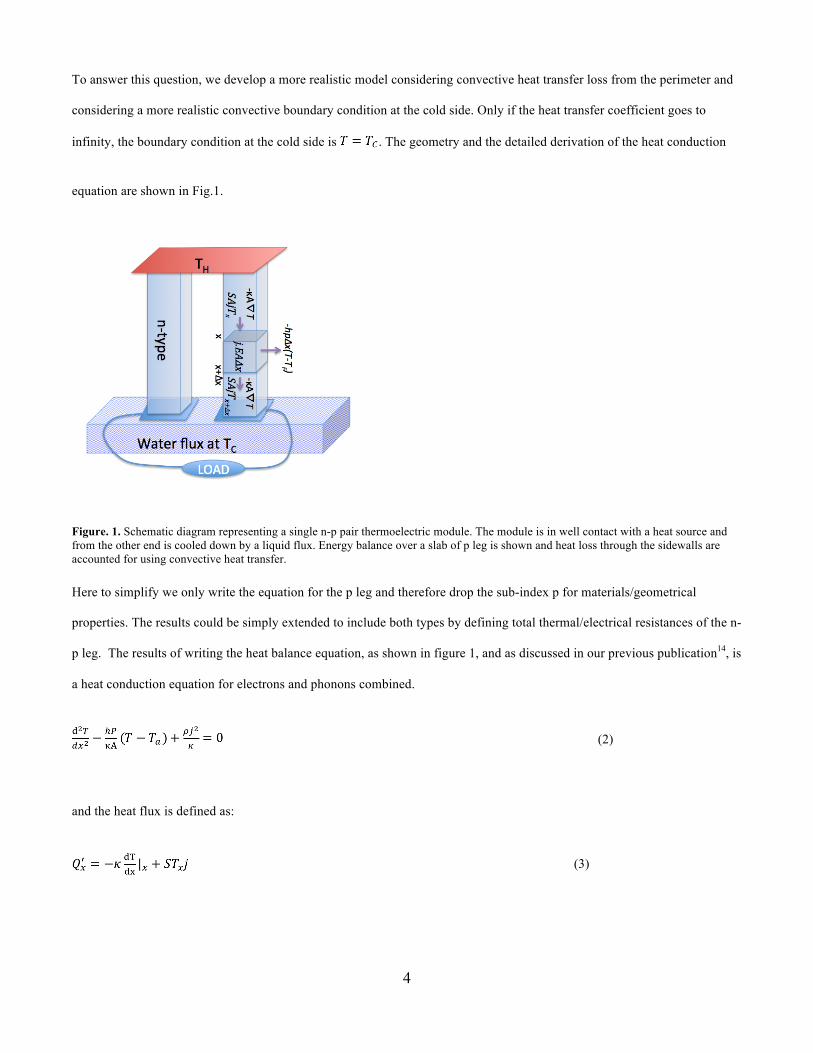
To answer this question, we develop a more realistic model considering convective heat transfer loss from the perimeter and

considering a more realistic convective boundary condition at the cold side. Only if the heat transfer coefficient goes to

infinity, the boundary condition at the cold side is . The geometry and the detailed derivation of the heat conduction

equation are shown in Fig.1.

Figure. 1. Schematic diagram representing a single n-p pair thermoelectric module. The module is in well contact with a heat source and from the other end is cooled down by a liquid flux. Energy balance over a slab of p leg is shown and heat loss through the sidewalls are accounted for using convective heat transfer.

Here to simplify we only write the equation for the p leg and therefore drop the sub-index p for materials/geometrical

properties. The results could be simply extended to include both types by defining total thermal/electrical resistances of the n-

p leg. The results of writing the heat balance equation, as shown in figure 1, and as discussed in our previous publication14, is

a heat conduction equation for electrons and phonons combined.

(2)

and the heat flux is defined as:

(3)

5

is the leg perimeter, A is the cross section of the leg, is the ambient temperature, is the total thermal conductivity due

to electrons and phonons, and is the electric current flux. The main approximation here is that temperature is constant in the

y-z plane. Note that this assumption is used very often in modeling of fins.15,16 Also note that in Eq. 2, we are neglecting the

Thomson effect to simplify the solutions. In other words, we assume that the Seebeck coefficient is not changing with

temperature ( ). Full solutions with inclusion of Thomson terms, are too lengthy and it is hard to extract information

from such complicated equations.12,17

To further simplify the solutions, we define a set of dimensionless parameters and we also change the reference for

measuring the temperature:

(4a)

(4b)

(4c)

(4d)

(4e)

is a dimensionless current, is similar to the Biot number, defined at the cold end with being the length of the

thermoelectric leg and , the thermal conductivity of the TE module. is representative of the effectiveness of cooling at

the cold side. Larger values correspond to larger values and therefore better cooling at the cold end. is another

dimensionless parameter, which is known as the fin parameter. In this analysis, it is the representative of heat loss through

sidewalls and increases as (the heat transfer coefficient through the sidewalls) increases.

6

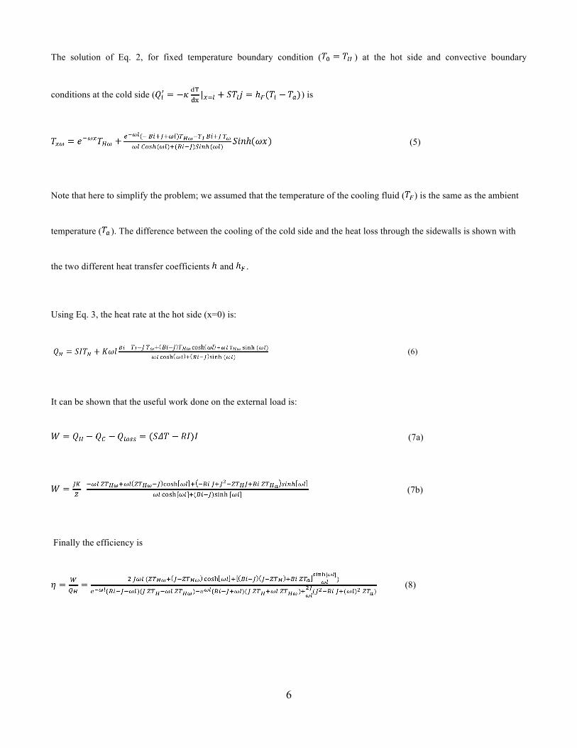
The solution of Eq. 2, for fixed temperature boundary condition ( ) at the hot side and convective boundary

conditions at the cold side ( ) is

(5)

Note that here to simplify the problem; we assumed that the temperature of the cooling fluid ( ) is the same as the ambient

temperature ( ). The difference between the cooling of the cold side and the heat loss through the sidewalls is shown with

the two different heat transfer coefficients and .

Using Eq. 3, the heat rate at the hot side (x=0) is:

(6)

It can be shown that the useful work done on the external load is:

(7a)

(7b)

Finally the efficiency is

(8)

7

Results

To look at a practical device performance, we take dimensions from a typical thermoelectric module. For example those of

the HZ-14 discussed earlier in the introduction and is summarized in caption of Fig.2.

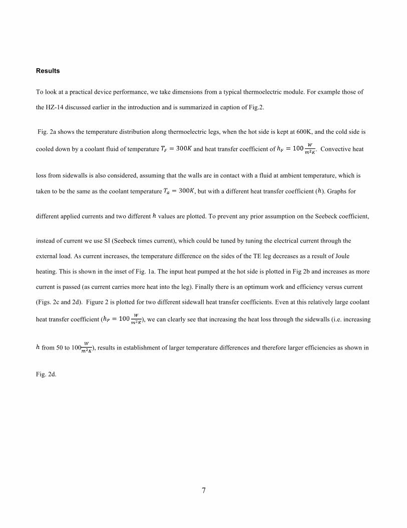
Fig. 2a shows the temperature distribution along thermoelectric legs, when the hot side is kept at 600K, and the cold side is

cooled down by a coolant fluid of temperature and heat transfer coefficient of . Convective heat

loss from sidewalls is also considered, assuming that the walls are in contact with a fluid at ambient temperature, which is

taken to be the same as the coolant temperature , but with a different heat transfer coefficient ( ). Graphs for

different applied currents and two different values are plotted. To prevent any prior assumption on the Seebeck coefficient,

instead of current we use SI (Seebeck times current), which could be tuned by tuning the electrical current through the

external load. As current increases, the temperature difference on the sides of the TE leg decreases as a result of Joule

heating. This is shown in the inset of Fig. 1a. The input heat pumped at the hot side is plotted in Fig 2b and increases as more

current is passed (as current carries more heat into the leg). Finally there is an optimum work and efficiency versus current

(Figs. 2c and 2d). Figure 2 is plotted for two different sidewall heat transfer coefficients. Even at this relatively large coolant

heat transfer coefficient ( ), we can clearly see that increasing the heat loss through the sidewalls (i.e. increasing

from 50 to 100 ), results in establishment of larger temperature differences and therefore larger efficiencies as shown in

Fig. 2d.

8

Figure. 2. Results for a single p-n pair, the dimensions are ,

. Black lines are plotted for and green lines for

. a) Temperature distribution along the thermoelectric leg for different SI values which is increased from 0 to 2 with steps

of and using Eq. 5. Inset: as a function of SI (in units). b) Input heat current (heat current at the hot side, , Eq.

6) as a function of SI, c) Useful output work (Eq. 7) as a function of SI and d) Efficiency of heat to electricity conversion (Eq.8) as a function of SI.

We know at the limit of , the results will be completely different and larger values, result in more heat loss and less

efficiency. So the next natural question is that how large is large enough to be considered as the limit of infinity and when we

will switch from gaining by opening heat loss channels to loosing by opening such channels. To answer this question, we

note that for a fixed set of temperatures, efficiency is a function of 4 different parameters namely Z, J, and (see Eq. 8).

Among these parameters, J is irrelevant in the sense that it is tunable and for a given thermoelectric module, we can optimize

the efficiency versus this parameter. Z parameter could be fixed, as we know good commercial thermoelectric materials

possess values close to 1 and in the research labs this value is close to 2. The remaining two parameters, and , are

then the crucial parameters in our discussion. While represents the amount of heat loss from the sidewalls, , represents

the effectiveness of the cooling system used at the cold end. To find the transition point, we fixed the temperatures and the

9

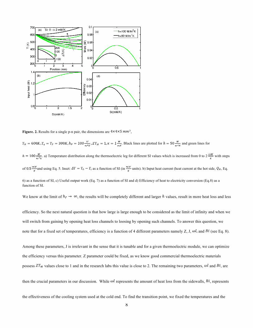
figure of merit. Then, for a given and , we optimized the efficiency versus J. The resulted optimum efficiency is plotted

in Fig.3. For the set of chosen parameters, the ideal efficiency, according to the Goldsmid analysis, Eq. 1, is about 10%. Fig.

3 shows that this ideal efficiency is only achievable for values larger than 8. For a thermal conductivity of 1W/mK,

and length of 5mm, this corresponds to . In this regime, as expected, any heat loss (increase of ) results in

lowering of the efficiency. The transition happens at around . Below this value, the efficiency increases as heat loss

through sidewalls increases (when increases), which is counter-intuitive and is happening due to the consequent

establishment of a larger temperature difference. The transition point could be more easily identified from Fig. 3b. In this

figure the derivative of the efficiency with respect to is plotted. This derivative is positive for small Bi values and is

negative for larger ones. The transition happens around . The absolute values of efficiency are sensitive to the chosen

temperatures (of the hot side and of the ambient/fluid) and the Z parameter. However, the overall shape of this graph (Fig. 3)

has only minor sensitivity to any of these parameters and therefore the value could be taken as the transition value

independent of the Z and the temperature values. In fact, the overall result of increasing Z parameter and temperature

difference is to shift the transition point slightly to larger values. Which means for larger ZT values, even larger values are

required for efficient heat conversion. The studied case of Fig.2 was corresponding to which is clearly in the regime

wherein heat loss through sidewalls is beneficial.

10

Figure 3. a) Optimum efficiency versus , and , plotted for . Ideal efficiency (from Eq. 1)

for the set of chosen parameters is 10%. b) The derivative of efficiency with respect to using the same parameters as in part a)

Conclusions

In summary, we developed a fin model for thermoelectric power generators, including the convective heat transfer

coefficient from the sidewalls. We determined that in addition to the Z parameter and the temperatures, the device efficiency

is also a function of two dimensionless parameters. One is ( , Biot number) which represents the effectiveness of the

cooling system used through value and the other is ( , fin parameter) which represents the heat loss through

side walls. We showed that if , that is when poor cooling is used at the cold side, opening heat loss channels through

the sidewalls, increases the overall efficiency of the thermoelectric module as a result of formation of a larger temperature

difference over the thermoelectric legs. In the opposite regime, when , we recovered the normal predicted behavior of

thermoelectrics, where in extra heat loss result in lowing of the heat to electricity conversion efficiency.

Acknowledgements

MZ would like to acknowledge K. Esfarjani for his helpful feedback on the manuscript. This work is supported by the

Air Force young investigator award, grant number FA9550-14-1-0316.

References

             1. Ioffe, A. F. Semiconductor thermoelements, and Thermoelectric cooling. (Infosearch, ltd., 1957).

2. Goldsmid, H. J. in Semiconductors and Semimetals (ed. Tritt, T.) 69, 1–24 (Academic Press, 2001).

3. Yazawa, K. et al. Thermoelectric topping cycles for power plants to eliminate cooling water consumption. Energy Convers. Manag. 84, 244–252 (2014).

4. Bell, L. E. Cooling, heating, generating power, and recovering waste heat with thermoelectric systems. Science 321, 1457–61 (2008).

5. Chen, J. Thermodynamic analysis of a solar-driven thermoelectric generator. 79, 2717–2721 (1996).

6. Xi, H., Luo, L. & Fraisse, G. Development and applications of solar-based thermoelectric

11

technologies. 11, 923–936 (2007).

7. Kraemer, D., Poudel, B. & Feng, H.-P. High-performance flat-panel solar thermoelectric generators with high thermal concentration. 10, 532–538 (2011).

8. Hi-Z14 thermoelectric module. Available at <http://www.hi-z.com/hz-14.html>

9. Nolas, G. S., Sharp, J. & Goldsmid, H. J. Thermoelectrics: Basic Principles and New Materials Developments. (Springer, 2001).

10. Xiao, H., Gou, X. & Yang, S. Detailed Modeling and Irreversible Transfer Process Analysis of a Multi-Element Thermoelectric Generator System. J. Electron. Mater. 40, 1195–1201 (2011).

11. Reddy, B. V. K., Barry, M., Li, J. & Chyu, M. K. Thermoelectric Performance of Novel Composite and Integrated Devices Applied to Waste Heat Recovery. J. Heat Transfer 135, 031706 (2013).

12. Rabari, R., Mahmud, S., Dutta, A. & Biglarbegian, M. Effect of Convection Heat Transfer on Performance of Waste Heat Thermoelectric Generator. Heat Transf. Eng. 36, 1458–1471 (2015).

13. Goldsmid, H. J. Introduction to Thermoelectricity (Springer Series in Materials Science). (Springer, 2009).

14. Zebarjadi, M. Electronic cooling using thermoelectric devices. Appl. Phys. Lett. 106, 203506 (2015).

15. Y.A., C. & AJ, G. Heat and Mass Transfer Fundamentals & Applications. (McGraw-Hill, 2015).

16. Bergman, T. L., Lavine, A. S., Incropera, F. P. & DeWitt, D. P. Introduction to Heat Transfer. (John Wiley and Sons, Inc., 2011).

17. Fraisse, G., Lazard, M., Goupil, C. & Serrat, J. Y. Study of a thermoelement’s behaviour through a modelling based on electrical analogy. Int. J. Heat Mass Transf. 53, 3503–3512 (2010).