Embed Size (px)
Citation preview
December, 2002 International Commission of Agricultural Engineering, Section II
4th Report of Working Group
on
Climatization of Animal Houses Heat and moisture production
at animal and house levels
Editors: Pedersen, S. & Sällvik, K.
2002
Published by Research Centre Bygholm, Danish Institute of Agricultural Sciences, P.O Box 536,
DK-8700 Horsens, Denmark
ISBN 87-88976-60-2
www.agrsci.dk/jbt/spe/CIGRreport

3
Contents
1. Preface........................................................................................................................................... 5 1.1 Members of the working group ........................................................................................... 6
2. Heat and moisture production at animal level .............................................................................. 8
2.1. Total heat production at 20oC.............................................................................................. 9 2.2. Cattle .................................................................................................................................. 10
2.2.1 Calves .................................................................................................................... 10 2.2.2 Veal calves, beef cattle .......................................................................................... 10 2.2.3 Heifers.................................................................................................................... 10 2.2.4 Cows ...................................................................................................................... 10
2.3 Pigs .................................................................................................................................... 10
2.3.1 Piglets .................................................................................................................... 10 2.3.2 Fattening pigs......................................................................................................... 11 2.3.3 Sows, boars and gilts ............................................................................................. 11 2.3.4 Nursing sows ......................................................................................................... 11
2.4 Horses ................................................................................................................................ 11 2.5 Sheep ................................................................................................................................. 12
2.5.1 Lamb ...................................................................................................................... 12 2.5.2 Breeding sheep....................................................................................................... 12
2.6 Goats .................................................................................................................................. 12 2.7 Poultry ............................................................................................................................... 12
2.7.1 Broilers .................................................................................................................. 12 2.7.2 Laying hens in cages.............................................................................................. 12 2.7.3 Laying hens on floors ............................................................................................ 12 2.7.4 Turkeys .................................................................................................................. 12
2.8 Rabbits ............................................................................................................................... 13 2.9 Mink .................................................................................................................................. 13
2.9.1 Females with 6 kids ............................................................................................... 13 2.9.2 Males...................................................................................................................... 13
2.10 Total heat production at temperatures different from 20oC............................................... 13 2.11 Partitioning between sensible and latent heat dissipation ................................................. 18
4
3. Heat and moisture production at house level.............................................................................. 20 3.1 Cattle .................................................................................................................................. 22
3.1.1 Calves .................................................................................................................... 22 3.1.2 Heifers.................................................................................................................... 22 3.1.3 Dairy cows in tie-stall house and cubicles............................................................. 22 3.1.4 Dairy cows on deep litter....................................................................................... 24
3.2 Pigs .................................................................................................................................... 25
3.2.1 Weaners (See fattening pigs) ................................................................................. 25 3.2.2 Fattening pigs on partly slatted floor ..................................................................... 25
3.3 Poultry ............................................................................................................................... 25
3.3.1 Broilers on 50-100 mm litter ................................................................................. 25 3.3.2 Layers kept in cages............................................................................................... 26 3.3.3 Layers raised on floors........................................................................................... 27 3.3.4 Turkeys raised on litter .......................................................................................... 28
4. Diurnal variation in animal heat production............................................................................... 29
4.1 Diurnal variations in heat production for cattle................................................................. 29 4.2 Diurnal variations in heat production for pigs................................................................... 30 4.3 Diurnal variations in heat production for poultry.............................................................. 34
5. Carbon dioxide production.......................................................................................................... 37
5.1 Models for calculation of ventilation flow, based on indoor carbon dioxide concentrations .................................................................................................................... 37
6. Summary..................................................................................................................................... 41 7. References ................................................................................................................................... 42
5
1. Preface
A working group on Climatization of Animal Houses was founded in 1977 by CIGR (Commission
Internationale du Génie Rural) Section II, with Dr. Michael Rist, Switzerland as chairman. The main
goal for the group was to develop guidelines on animal heat and moisture production rates for proper
sizing and operation of ventilation and heating equipment for animal houses. The first report from the
group was published in 1984, and since then, it has served as guidelines in many countries. From the
very beginning, it has been a hard process to come up with a common calculation procedure, due to
different traditions among countries in the way of handling latent heat. Some countries used total heat
as basis for calculation of the ventilation flow requirement, with an adjustment for the share of latent
heat. Another obstacle was that each country had individual tables for animal heat and moisture
production and no clear indentification of to which indoor they corresponded. Other countries based
the ventilation flow requirement for heat and moisture balance directly on the partition of sensible and
latent heat at the inside design temperature. From an international viewpoint, the goal for the work was
to achieve a common reliable calculation procedure based on available knowledge. The 1984 report
was followed by Report II from 1989 (revised in 1992), which included ventilation principles, dust and
gases, as well as an improved equation for calculation of heat production of fattening pigs, taking into
account differences in feed intake. The third report from 1994 primarily dealt with aerial contaminants.
At a very early stage in the history of the working groups, it was clear that the available information on
heat and moisture production was mainly based on animal heat production, not taking into account
aspects like different feeding and housing systems. Water evaporated from feed, manure and wet
surfaces were not taken into account, because most of the results were obtained under laboratory
conditions. Owing to the lack of knowledge, it was not possible at that time to go further into detail
with heat and moisture production on a house level. However, already in the first report from 1984, it
was mentioned that the available information on heat and moisture production in confinement
buildings primarily covers the animal production issue. Furthermore, the report included provisional
recommendations for adjustments by using a correction factor, ks, for sensible heat. For cattle, the ks
was, for instance, set to 0.85 for "normal" housing conditions, corresponding to an increase in latent
heat of, e.g., 40% at an indoor temperature of 15oC. For wet and dry conditions, the ks for cows was set
to 0.8 and 0.9, respectively. It is obvious that an adjustment of the latent heat of 40% for cattle will
have a tremendous impact on, e.g., the validity of calculated indoor humidity compared to the real
indoor humidity. Also, for animal houses with a need of supplemental heat as, e.g, broiler houses, it is
very important to have reliable values for latent heat as well as sensible heat. Otherwise, estimations of
the heat requirements for maintaining a certain indoor relative humidity will be completely wrong.
Therefore, this report is focused on the heat and moisture production under practical conditions for
6
different kinds of animals and outdoor climate. Unfortunately, the experimental data for heat and
moisture levels are limited and primarily related to Northern European production and housing
conditions. The intention for the coming years is to gather practical figures, also for e.g. the European
Mediterranian area.
1.1 Members of the working group
Since the working group was founded in 1977, an annual meeting with about ten participants from
different countries has been held – primarily in Europe with corresponding members from, e.g. USA.
In the middle of the 1990's, the European organisation of AgEng established special interest groups
(SIG) within different areas, where SIG 14 is also dealing with climatization of animal houses.
Because the members of the CIGR working group and of the SIG 14 are more or less identical, the two
groups have gradually merged into a CIGR/SIG working group during the last couple of years. During
recent years, the meetings have primarily been held in connection with, e.g. symposiums or congresses,
and they have been openened to voluntary participants. Altogether, more than 50 different people have
participated in one or more meetings throughout the years, and they have contributed in many different
ways. The following people have contributed to this report:
Contributors
Dr. André Aarnink, IMAG, The Netherlands
Dr. Thomas Banhazi, Adelaide University, Australia
Mr. Bea, W., University of Hohenheim, Germany
Ir. Ludo van Caenegem, FAT, Switzerland
Dr. Jan Elnif, The Royal Veterinary and Agricultural University, Denmark
Dr. Marcella Guarino, Milano University, Italy
Dr. Gösta Gustafsson, Swedish University of Agricultural Sciences, Sweden
Dr. Knut-Hakan Jeppsson, Swedish University of Agricultural Sciences, Sweden
Dr. Henry Jørgensen, DIAS, Denmark
Mr. Svend Morsing, DIAS, Denmark
Dr. Søren Pedersen, DIAS, Denmark (secretary for the working group)
Dr. Hans Benny Rom, DIAS, Denmark
Professor Krister Sällvik, Swedish University of Agricultural Sciences, Sweden (chairman for the
working group)
Mr. P. Theil, DIAS, Denmark
Ms. Eva von Wachenfelt, Swedish University of Agricultural Sciences, Sweden
Dr. H. Xin, professor, Iowa State University, Ames, Iowa, USA
7
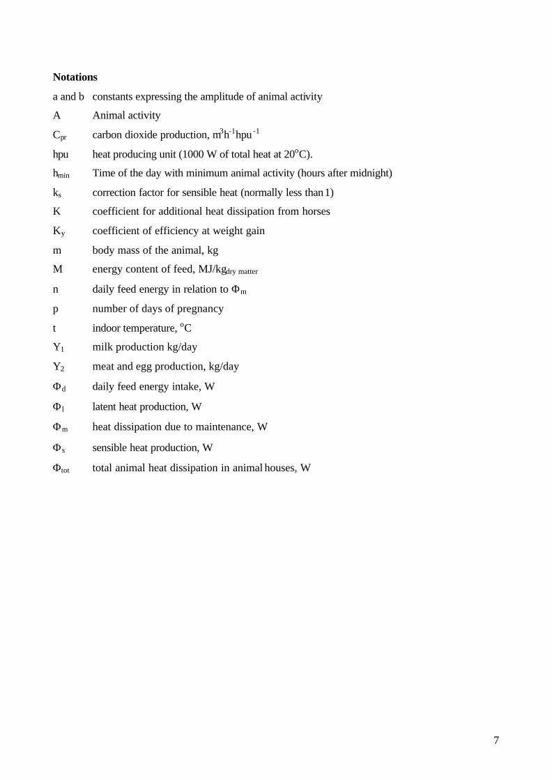
Notations
a and b constants expressing the amplitude of animal activity
A Animal activity
Cpr carbon dioxide production, m3h-1hpu -1
hpu heat producing unit (1000 W of total heat at 20oC).
hmin Time of the day with minimum animal activity (hours after midnight)
ks correction factor for sensible heat (normally less than 1)
K coefficient for additional heat dissipation from horses
Ky coefficient of efficiency at weight gain
m body mass of the animal, kg
M energy content of feed, MJ/kgdry matter
n daily feed energy in relation to Φm
p number of days of pregnancy
t indoor temperature, oC
Y1 milk production kg/day
Y2 meat and egg production, kg/day
Φd daily feed energy intake, W
Φl latent heat production, W
Φm heat dissipation due to maintenance, W
Φs sensible heat production, W
Φtot total animal heat dissipation in animal houses, W
8
2. Heat and moisture production at animal level
The total animal heat production will fundamentally depend on the fact that animals are
homothermal and full heat producing, because their heat production due to maintenance and
production must be dissipated from their bodies. Consequently, their body weights and production
levels, i.e. their feed intake, will influence their total heat production directly. How the heat is
dissipated will depend on the physiology of the animals and on the surround ings with respect to air
temperature, radiation from cold/warm surfaces, air velocity and bedding conditions. Furthermore,
animal heat production varies diurnally as a consequence of the animal activity influenced by
feeding routines and photoperiod (light vs.darkness). Therefore, it is important to define for which
condition the animal heat production is referred. In accordance with common practice, 20oC and
"normal" production conditions on a 24-hour basis are selected as benchmarks for all species.
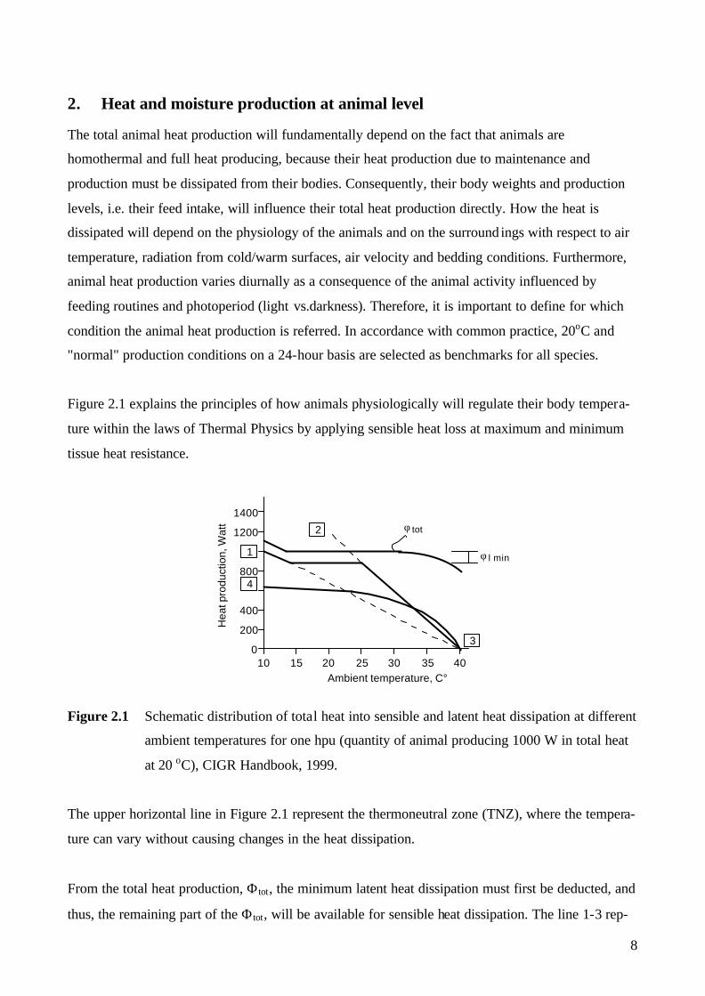
Figure 2.1 explains the principles of how animals physiologically will regulate their body tempera-
ture within the laws of Thermal Physics by applying sensible heat loss at maximum and minimum
tissue heat resistance.
Figure 2.1 Schematic distribution of total heat into sensible and latent heat dissipation at different
ambient temperatures for one hpu (quantity of animal producing 1000 W in total heat
at 20 oC), CIGR Handbook, 1999.
The upper horizontal line in Figure 2.1 represent the thermoneutral zone (TNZ), where the tempera-
ture can vary without causing changes in the heat dissipation.
From the total heat production, Φtot, the minimum latent heat dissipation must first be deducted, and
thus, the remaining part of the Φtot, will be available for sensible heat dissipation. The line 1-3 rep-
10 15 20 25 30 35 400
200
1400
1200
800
400
3
4
1
2
Ambient temperature, C°
Hea
t pro
duct
ion,
Wat
t φ tot
φ l min
9
represents the sensible heat dissipation at maximum tissue resistance. The point (temperature)
where the heat dissipation resistance equals (Φtot - Φlmin ) according to the maximum tissue resis-
tance is the lower critical temperature (LCT). At temperatures below, the LCT, Φtot, must increase,
so that the animals can maintain their body temperature.
The point (temperature) where the sensible heat loss at minimum tissue resistance represented by
lines 2-3 is not sufficient to balance the heat production and the latent heat must increase. For the
upper critical temperature, no clear definition exists, as for the lower one. In reality, animals per-
form a much smoother transfer between these principles of thermoregulation of their body tempera-
tures.
2.1. Total heat production at 20oC
All farm animals are homeothermal and must keep their body temperature reasonably constant. The
animals dissipate heat, partly as a result of maintaining essential functions (Φm maintenance) and
partly due to their productivity. Under thermoneutral conditions (20°C) for most adult farm
animals), the total heat dissipation from an animal, Φtot, mainly depends on:
• Body mass
• Production and activity level (milk, meat, eggs, foetuses)
• Proportion between lean and fat tissue gains
• Energy concentration in the feed
Equations for total heat production,Φtot
The equations for total heat production rate under thermoneutrality, Φtot, presented below are based
on CIGR (1984), CIGR (1992), Swedish Standard (1992), CIGR Handbook, 1999, and data from a
recent literature review for poultry heat and moisture production (Chepete and Xin, 2002).
The first part of the equations gives the heat dissipation due to maintenance, Φm, and is a function
of the metabolic body mass weight. For example for cows, the maintenance, Φm, is 5.6 m0.75.
10
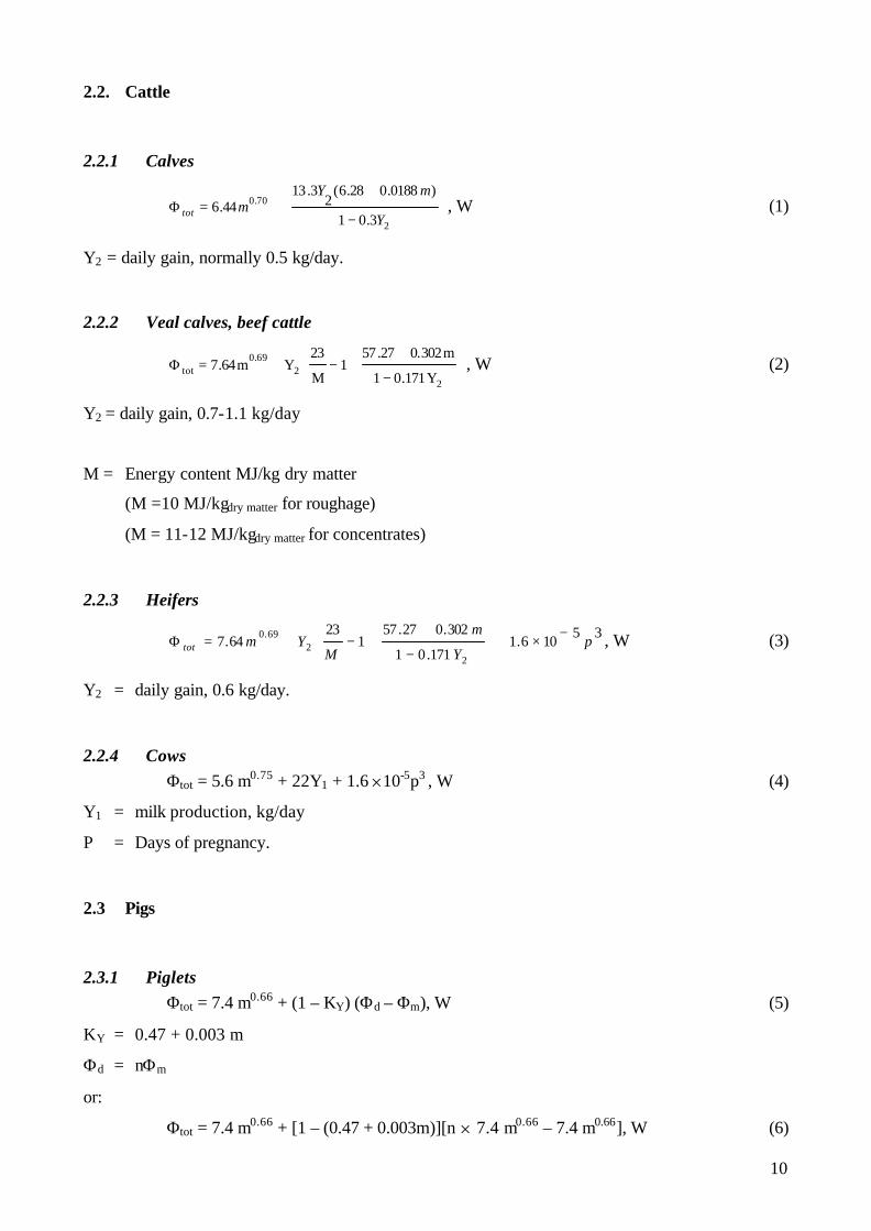
2.2. Cattle
2.2.1 Calves
−
++=Φ
2
70.0
3.01
)0188.028.6(2
3.1344.6
Y
mYmtot , W (1)
Y2 = daily gain, normally 0.5 kg/day.
2.2.2 Veal calves, beef cattle
−
+−+=Φ
22
69.0tot Y171.01
m302.027.571
M
23Ym64.7 , W (2)
Y2 = daily gain, 0.7-1.1 kg/day
M = Energy content MJ/kg dry matter
(M =10 MJ/kgdry matter for roughage)
(M = 11-12 MJ/kgdry matter for concentrates)
2.2.3 Heifers
35106.1171.01
302.027.571
2364.7
22
69.0 pY
m
MYmtot
−×+−
+−+=Φ
, W (3)
Y2 = daily gain, 0.6 kg/day.
2.2.4 Cows Φtot = 5.6 m0.75 + 22Y1 + 1.6 510-5p3 , W (4)
Y1 = milk production, kg/day
P = Days of pregnancy.
2.3 Pigs
2.3.1 Piglets Φtot = 7.4 m0.66 + (1 – KY) (Φd – Φm), W (5)
KY = 0.47 + 0.003 m
Φd = nΦm
or:
Φtot = 7.4 m0.66 + [1 – (0.47 + 0.003m)][n 5 7.4 m0.66 – 7.4 m0.66], W (6)
11
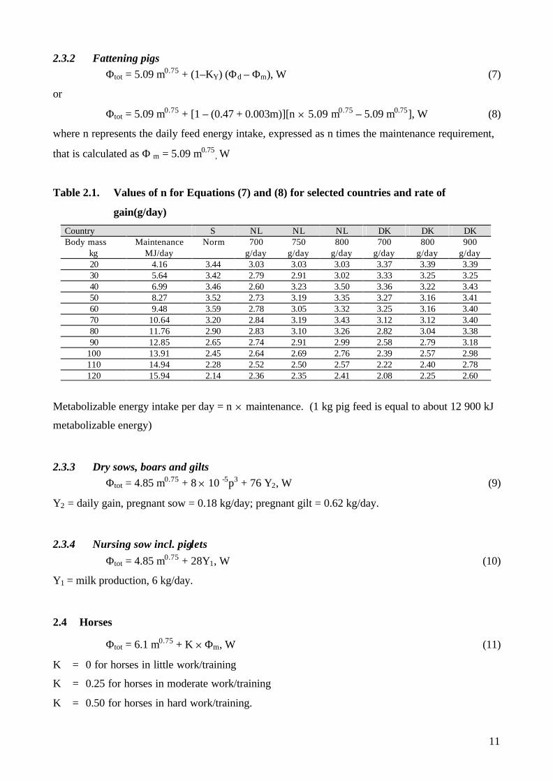
2.3.2 Fattening pigs Φtot = 5.09 m0.75 + (1–KY) (Φd – Φm), W (7)
or
Φtot = 5.09 m0.75 + [1 – (0.47 + 0.003m)][n 5 5.09 m0.75 – 5.09 m0.75], W (8)
where n represents the daily feed energy intake, expressed as n times the maintenance requirement,
that is calculated as Φ m = 5.09 m0.75, W
Table 2.1. Values of n for Equations (7) and (8) for selected countries and rate of
gain(g/day)
Country S NL NL NL DK DK DK Body mass
kg Maintenance
MJ/day Norm 700
g/day 750
g/day 800
g/day 700
g/day 800
g/day 900
g/day 20 4.16 3.44 3.03 3.03 3.03 3.37 3.39 3.39 30 5.64 3.42 2.79 2.91 3.02 3.33 3.25 3.25 40 6.99 3.46 2.60 3.23 3.50 3.36 3.22 3.43 50 8.27 3.52 2.73 3.19 3.35 3.27 3.16 3.41 60 9.48 3.59 2.78 3.05 3.32 3.25 3.16 3.40 70 10.64 3.20 2.84 3.19 3.43 3.12 3.12 3.40 80 11.76 2.90 2.83 3.10 3.26 2.82 3.04 3.38 90 12.85 2.65 2.74 2.91 2.99 2.58 2.79 3.18
100 13.91 2.45 2.64 2.69 2.76 2.39 2.57 2.98 110 14.94 2.28 2.52 2.50 2.57 2.22 2.40 2.78 120 15.94 2.14 2.36 2.35 2.41 2.08 2.25 2.60
Metabolizable energy intake per day = n 5 maintenance. (1 kg pig feed is equal to about 12 900 kJ
metabolizable energy)
2.3.3 Dry sows, boars and gilts Φtot = 4.85 m0.75 + 8 5 10 -5p3 + 76 Y2, W (9)
Y2 = daily gain, pregnant sow = 0.18 kg/day; pregnant gilt = 0.62 kg/day.
2.3.4 Nursing sow incl. piglets Φtot = 4.85 m0.75 + 28Y1, W (10)
Y1 = milk production, 6 kg/day.
2.4 Horses
Φtot = 6.1 m0.75 + K 5 Φm, W (11)
K = 0 for horses in little work/training
K = 0.25 for horses in moderate work/training
K = 0.50 for horses in hard work/training.
12
2.5 Sheep
2.5.1 Lamb Φtot = 6.4 m0.75 + 145Y2, W (12)
Y2 = daily gain, 0.25 kg/day.
2.5.2 Breeding sheep Φtot = 6.4 m0.75 + 33Y1 + 2.4 5 10-5 p3, W (13)
Y1 = milk production, nursing ewes = 1 to 1.5 kg/d.
2.6 Goats
Small goats Φtot = 6.3 m0.75, W (14)
Milking goats Φtot = 5.5 m0.75 + 13Y1, W (15)
Y1 = milk production, kg/day.
2.7 Poultry
2.7.1 Broilers Φtot = 10.62 m0.75 (16)
2.7.2 Laying hens in cages Φtot = 6.28 m0.75 +25 Y2, W (17)
Y2 = Egg production, kg/day.
(Y2 = 0.050 kg/day for consumer eggs)
(Y2 = 0.040 kg/day for brooding production)
2.7.3 Laying hens on floors Φtot = 6.8 m0.75 + 25Y2, W (18)
2.7.4 Turkeys Φtot = 9.86 m0.77, W (19)
13
2.8 Rabbits
Weight Φtot (20)
Fatteners 0.5 kg 3.9 W “ 1.5 kg 7.8 W “ 2.5 kg 12.1 W Adults 4.0 kg 17.6 W “ 5.0 kg 20.4 W 2.9 Mink
2.9.1 Females with 6 kids Φtot = 8 m0.75, W (21)
2.9.2 Males Φtot = 8 m0.75, W (22)
A recent review and analysis of literature data on heat and moisture production of poultry revealed
the evolutionary changes in total heat production, as shown in Table 2.2.
Table 2.2. Comparative models of total heat production (Φtot) of poultry at thermoneutrality
during different time periods of the past five decades (Chepete and Xin, 2002)
Poultry Species Year(s) Φtot (W/bird)
1968 8.55 M0.74 Broilers
1982-2000 10.62 M0.75
Pullets & Layers 1953-1990 6.47 M0.77
1974-1977 7.54 M0.53 Turkeys
1992-1998 9.86 M0.77
2.10 Total heat production at temperatures different from 20oC
The equations for calculation of Φtot refers to thermoneutral conditions (20oC) for most adult farm
animals. At lower temperatures, the total heat production increases, and at higher temperatures it
decreases. Due to lack of sufficient information for different species, a modified Equation (23) by
Strøm (1978) and CIGR (1984) has been used for all species and ages, on the basis of heat
producing units (hpu), where one hpu corresponds to 1000 W of total heat at 20°C.
Φtot = 1000 [1 + 4 5 10-5 (20 – t) 3], W (23)
14
The disadvantages of the above equation is that it neither takes the kind nor the size of the animal or
the production level into account. For instance, it shows that the total heat production increases by
100% when the ambient at temperature decreases from 20oC to -10oC, which is unlikely for cattle
that will only respond very little to ambient temperatures. Another disadvantage of Equation (23) is
that it is based on the assumption that a thermoneutral zone clearly exists, which was not confirmed
by a literature survey, as shown below.
The 2001 ASHRAE Handbook –Fundamentals (ASHRAE, 2001a) refers to the results from
different experiments with cattle, pigs and poultry.
Expressed with respect to 20oC for a hpu, the relations between the ambient temperature and the
total heat production for cattle and pigs are as shown in Figures 2.1, 2.2 and 2.4.
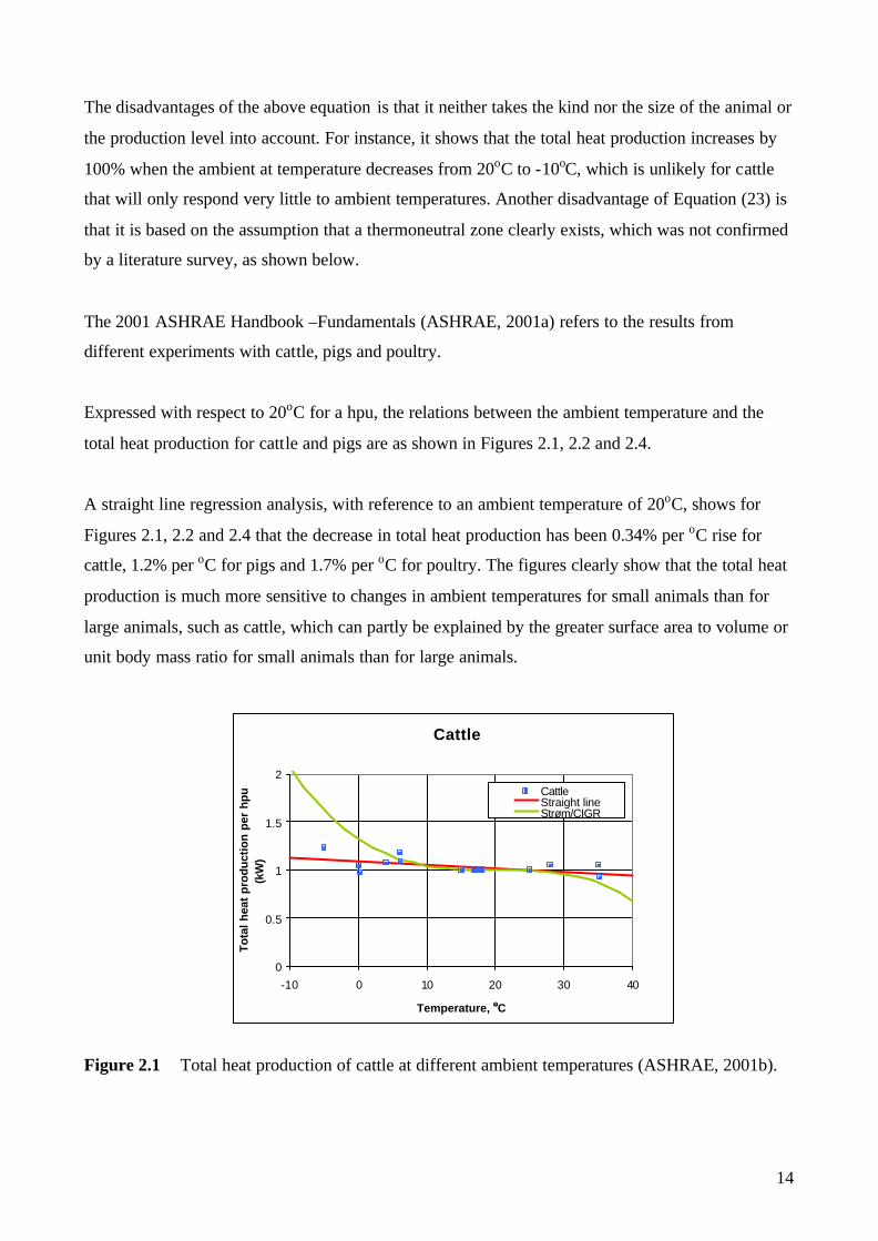
A straight line regression analysis, with reference to an ambient temperature of 20oC, shows for
Figures 2.1, 2.2 and 2.4 that the decrease in total heat production has been 0.34% per oC rise for
cattle, 1.2% per oC for pigs and 1.7% per oC for poultry. The figures clearly show that the total heat
production is much more sensitive to changes in ambient temperatures for small animals than for
large animals, such as cattle, which can partly be explained by the greater surface area to volume or
unit body mass ratio for small animals than for large animals.
Figure 2.1 Total heat production of cattle at different ambient temperatures (ASHRAE, 2001b).
Cattle
Based on ASHRAE Standard 2001
0
0.5
1
1.5
2
-10 0 10 20 30 40
Temperature, oC
Tota
l hea
t pr
oduc
tion
per
hpu
(kW
)
CattleStraight lineStrøm/CIGR
15
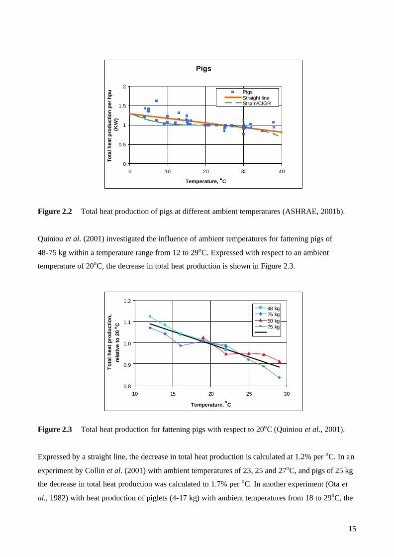
Figure 2.2 Total heat production of pigs at different ambient temperatures (ASHRAE, 2001b).
Quiniou et al. (2001) investigated the influence of ambient temperatures for fattening pigs of
48-75 kg within a temperature range from 12 to 29oC. Expressed with respect to an ambient
temperature of 20oC, the decrease in total heat production is shown in Figure 2.3.
Figure 2.3 Total heat production for fattening pigs with respect to 20oC (Quiniou et al., 2001).
Expressed by a straight line, the decrease in total heat production is calculated at 1.2% per oC. In an
experiment by Collin et al. (2001) with ambient temperatures of 23, 25 and 27oC, and pigs of 25 kg
the decrease in total heat production was calculated to 1.7% per oC. In another experiment (Ota et
al., 1982) with heat production of piglets (4-17 kg) with ambient temperatures from 18 to 29oC, the
0.8
0.9
1.0
1.1
1.2
10 15 20 25 30
Temperature, oC
To
tal h
eat
pro
du
ctio
n,
rela
tive
to 2
0 oC
48 kg75 kg50 kg75 kg
PigsBased on ASHRAE Standard 2001
0
0.5
1
1.5
2
0 10 20 30 40
Temperature, oC
Tota
l hea
t pr
oduc
tion
per
hpu
(KW
)
PigsStraight lineStrøm/CIGR
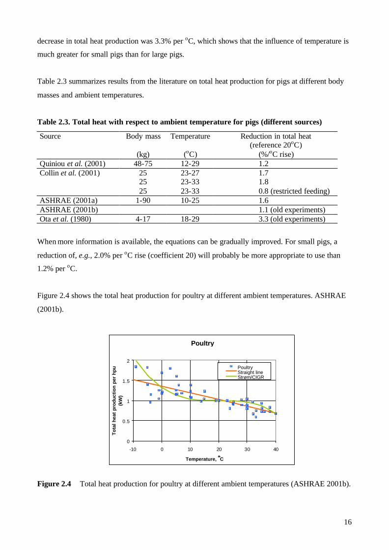
16
decrease in total heat production was 3.3% per oC, which shows that the influence of temperature is
much greater for small pigs than for large pigs.
Table 2.3 summarizes results from the literature on total heat production for pigs at different body
masses and ambient temperatures.
Table 2.3. Total heat with respect to ambient temperature for pigs (different sources)
Source Body mass
(kg)
Temperature
(oC)
Reduction in total heat (reference 20oC)
(%/oC rise) Quiniou et al. (2001) 48-75 12-29 1.2 Collin et al. (2001)
25 25 25
23-27 23-33 23-33
1.7 1.8 0.8 (restricted feeding)
ASHRAE (2001a) 1-90 10-25 1.6 ASHRAE (2001b) 1.1 (old experiments) Ota et al. (1980) 4-17 18-29 3.3 (old experiments)
When more information is available, the equations can be gradually improved. For small pigs, a
reduction of, e.g., 2.0% per oC rise (coefficient 20) will probably be more appropriate to use than
1.2% per oC.
Figure 2.4 shows the total heat production for poultry at different ambient temperatures. ASHRAE
(2001b).
Figure 2.4 Total heat production for poultry at different ambient temperatures (ASHRAE 2001b).
Poultry
Based on ASHRAE Standard 2001
0
0.5
1
1.5
2
-10 0 10 20 30 40
Temperature, oC
To
tal h
eat
pro
du
ctio
n p
er h
pu
(kW
)
PoultryStraight lineStrøm/CIGR
17
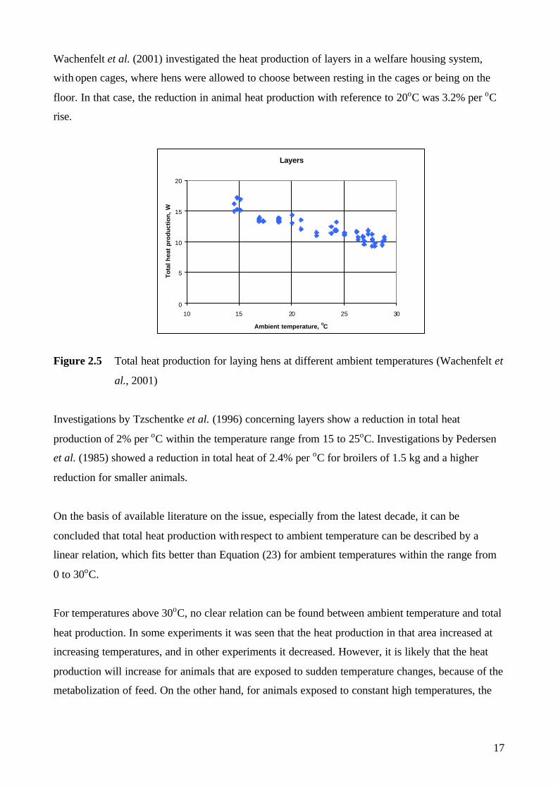
Wachenfelt et al. (2001) investigated the heat production of layers in a welfare housing system,
with open cages, where hens were allowed to choose between resting in the cages or being on the
floor. In that case, the reduction in animal heat production with reference to 20oC was 3.2% per oC
rise.
Figure 2.5 Total heat production for laying hens at different ambient temperatures (Wachenfelt et
al., 2001)
Investigations by Tzschentke et al. (1996) concerning layers show a reduction in total heat
production of 2% per oC within the temperature range from 15 to 25oC. Investigations by Pedersen
et al. (1985) showed a reduction in total heat of 2.4% per oC for broilers of 1.5 kg and a higher
reduction for smaller animals.
On the basis of available literature on the issue, especially from the latest decade, it can be
concluded that total heat production with respect to ambient temperature can be described by a
linear relation, which fits better than Equation (23) for ambient temperatures within the range from
0 to 30oC.
For temperatures above 30oC, no clear relation can be found between ambient temperature and total
heat production. In some experiments it was seen that the heat production in that area increased at
increasing temperatures, and in other experiments it decreased. However, it is likely that the heat
production will increase for animals that are exposed to sudden temperature changes, because of the
metabolization of feed. On the other hand, for animals exposed to constant high temperatures, the
Layers
0
5
10
15
20
10 15 20 25 30
Ambient temperature, oC
To
tal
hea
t p
rod
uct
ion
, W
18
feed intake is likely to be reduced, thus resulting in a lower heat production. It is therefore assumed
that a linear relation will be acceptable also for ambient temperatures above 30oC.
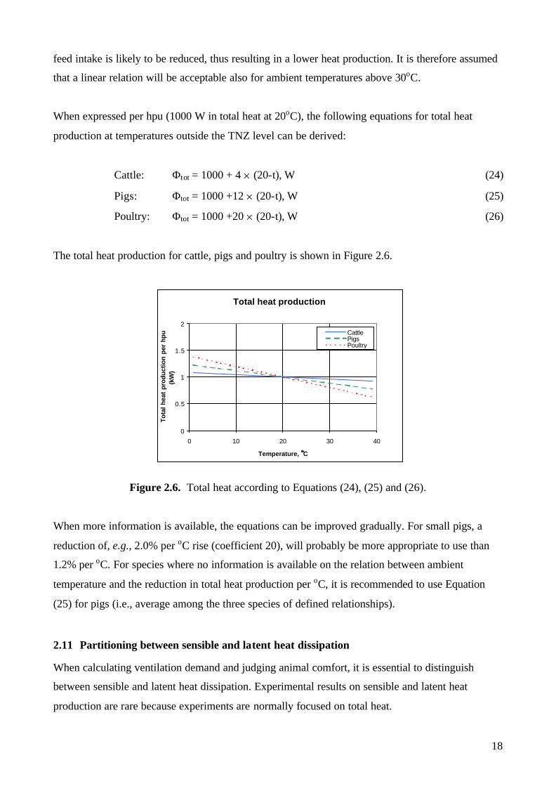
When expressed per hpu (1000 W in total heat at 20oC), the following equations for total heat
production at temperatures outside the TNZ level can be derived:
Cattle: Φtot = 1000 + 4 5 (20-t), W (24)
Pigs: Φtot = 1000 +12 5 (20-t), W (25)
Poultry: Φtot = 1000 +20 5 (20-t), W (26)
The total heat production for cattle, pigs and poultry is shown in Figure 2.6.
Figure 2.6. Total heat according to Equations (24), (25) and (26).
When more information is available, the equations can be improved gradually. For small pigs, a
reduction of, e.g., 2.0% per oC rise (coefficient 20), will probably be more appropriate to use than
1.2% per oC. For species where no information is available on the relation between ambient
temperature and the reduction in total heat production per oC, it is recommended to use Equation
(25) for pigs (i.e., average among the three species of defined relationships).
2.11 Partitioning between sensible and latent heat dissipation
When calculating ventilation demand and judging animal comfort, it is essential to distinguish
between sensible and latent heat dissipation. Experimental results on sensible and latent heat
production are rare because experiments are normally focused on total heat.
Total heat production
0
0.5
1
1.5
2
0 10 20 30 40
Temperature, oC
To
tal h
eat
pro
du
ctio
n p
er h
pu
(kW
)
CattlePigsPoultry
19
Φtot = Φs + Φl, W (27)
Φs is dissipated in accordance with the temperature gradient between the animal deep body
temperature and the ambient environment. Consequently, Φs will therefore be zero when the
ambient temperature is equal to the animal deep body temperature, depending on species., age, and
ambient temperature level.
Φl dissipates from the animal in the form of moisture from the respiratory track and the skin. To
maintain the animal heat balance and the body temperature, Φl will increase with increasing
temperature to substitute the decrease in Φs. The partitioning between Φs and Φl is furthermore
affected by factors such as type of animal, production stage, body surface area, fur type, dryness of
skin, and sweating ability.
The portioning of Φtot into Φs and Φ1 for different species and different housing conditions is
further discussed in chapter 3.
20
3. Heat and moisture production at house level
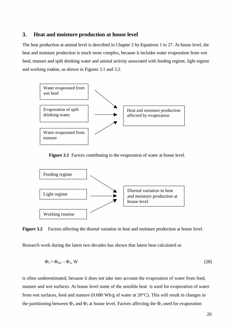
The heat production at animal level is described in Chapter 2 by Equations 1 to 27. At house level, the
heat and moisture production is much more complex, because it includes water evaporation from wet
feed, manure and spilt drinking water and animal activity associated with feeding regime, light regime
and working routine, as shown in Figures 3.1 and 3.2.
Figure 3.1 Factors contributing to the evaporation of water at house level.
Figure 3.2 Factors affecting the diurnal variation in heat and moisture production at house level.
Research work during the latest two decades has shown that latent heat calculated as
Φl = Φtot – Φs, W (28)
is often underestimated, because it does not take into account the evaporation of water from feed,
manure and wet surfaces. At house level some of the sensible heat is used for evaporation of water
from wet surfaces, feed and manure (0.680 Wh/g of water at 20°C). This will result in changes in
the partitioning between Φs and Φl at house level. Factors affecting the Φs used for evaporation
Feeding regime
Light regime
Working routine
Diurnal variation in heatand moisture production athouse level
Water evaporated fromwet feed
Evaporation of spiltdrinking-water
Water evaporated frommanure
Heat and moisture productionaffected by evaporation
21
could be flooring system, stocking density, watering, moisture content of the feed and feeding
system, animal activity and relative humidity.
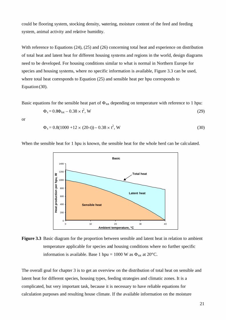
With reference to Equations (24), (25) and (26) concerning total heat and experience on distribution
of total heat and latent heat for different housing systems and regions in the world, design diagrams
need to be developed. For housing conditions similar to what is normal in Northern Europe for
species and housing systems, where no specific information is available, Figure 3.3 can be used,
where total heat corresponds to Equation (25) and sensible heat per hpu corresponds to
Equation (30).
Basic equations for the sensible heat part of Φtot depending on temperature with reference to 1 hpu:
Φs = 0.8Φtot – 0.38 5 t2, W (29)
or
Φs = 0.8(1000 +12 5 (20-t)) – 0.38 5 t2, W (30)
When the sensible heat for 1 hpu is known, the sensible heat for the whole herd can be calculated.
Figure 3.3 Basic diagram for the proportion between sensible and latent heat in relation to ambient
temperature applicable for species and housing conditions where no further specific
information is available. Base 1 hpu = 1000 W as Φtot at 20°C.
The overall goal for chapter 3 is to get an overview on the distribution of total heat on sensible and
latent heat for different species, housing types, feeding strategies and climatic zones. It is a
complicated, but very important task, because it is necessary to have reliable equations for
calculation purposes and resulting house climate. If the available information on the moisture
Basic
0
200
400
600
800
1000
1200
1400
0 10 20 30 40
Ambient temperature, °C
Hea
t p
rod
uct
ion
per
hpu
, W
Sensible heat
Latent heat
Total heat
22
production is insufficient, the results of computerized ventilation programs will also fail. At the
present state-of-the-art, the results of animal heat and moisture production on house level are scarce
and mainly based on investigations carried out in Northern Europe representing production systems
that are typical for that particular region. If we e.g. look at the production systems for cattle in the
Alpine regions, differences normally occur in the use of much dryer feed, and consequently, the
potential for evaporation of water will be lower. Also, the water content in incoming air at specific
outdoor temperatures may differ from one region to the other, due to differences in precipitation,
etc. Hopefully, the present information on some production situations in Northern Europe will
encourage a promotion of knowledge within that specific area.
3.1 Cattle
3.1.1 Calves Calves are often kept in boxes for single animals or group housed with some bedding in confinement
buildings with partly slatted floors and natural ventilation. Experience and research have shown that
the greatest indoor climate problem in calf houses in Northern Europe is the excessive indoor relative
humidity due to the relatively small amount of sensible heat available in the building and a high water
vapour evaporation from feed, drinking water, and manure, which restricts the ventilation rate (if no
additional heat). Due to lack of research on heat and moisture balances under normal production
conditions, specific recommendation for calves is not available. For heat and moisture production, see
Figure 3.4 on dairy cows.
3.1.2 Heifers See Figure 3.4
3.1.3 Dairy cows in tie-stall house and cubicles In the 1980's, some spot measurements of indoor relative humidity in houses for dairy cows were
carried out and compared to what could be expected from common calculation rules. The results
showed that measured indoor relative humidity was higher than what was calculated. For instance in
the CIGR 1984 report, the following table with provisional correction factors was given:
23
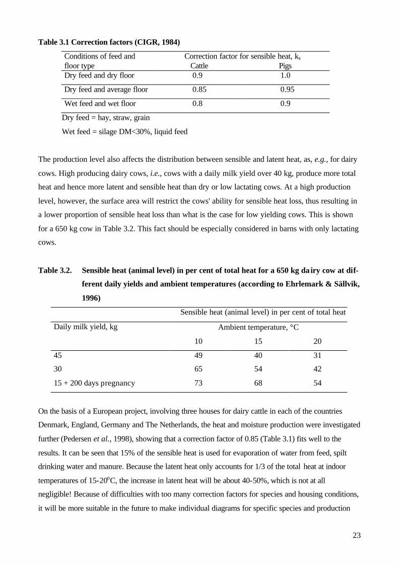
Table 3.1 Correction factors (CIGR, 1984)
Conditions of feed and floor type
Correction factor for sensible heat, ks
Cattle Pigs Dry feed and dry floor 0.9 1.0
Dry feed and average floor 0.85 0.95
Wet feed and wet floor 0.8 0.9
Dry feed = hay, straw, grain
Wet feed = silage DM<30%, liquid feed
The production level also affects the distribution between sensible and latent heat, as, e.g., for dairy
cows. High producing dairy cows, i.e., cows with a daily milk yield over 40 kg, produce more total
heat and hence more latent and sensible heat than dry or low lactating cows. At a high production
level, however, the surface area will restrict the cows' ability for sensible heat loss, thus resulting in
a lower proportion of sensible heat loss than what is the case for low yielding cows. This is shown
for a 650 kg cow in Table 3.2. This fact should be especially considered in barns with only lactating
cows.
Table 3.2. Sensible heat (animal level) in per cent of total heat for a 650 kg da iry cow at dif-
ferent daily yields and ambient temperatures (according to Ehrlemark & Sällvik,
1996)
Sensible heat (animal level) in per cent of total heat
Daily milk yield, kg Ambient temperature, °C
10 15 20
45 49 40 31
30 65 54 42
15 + 200 days pregnancy 73 68 54
On the basis of a European project, involving three houses for dairy cattle in each of the countries
Denmark, England, Germany and The Netherlands, the heat and moisture production were investigated
further (Pedersen et al., 1998), showing that a correction factor of 0.85 (Table 3.1) fits well to the
results. It can be seen that 15% of the sensible heat is used for evaporation of water from feed, spilt
drinking water and manure. Because the latent heat only accounts for 1/3 of the total heat at indoor
temperatures of 15-20oC, the increase in latent heat will be about 40-50%, which is not at all
negligible! Because of difficulties with too many correction factors for species and housing conditions,
it will be more suitable in the future to make individual diagrams for specific species and production
24
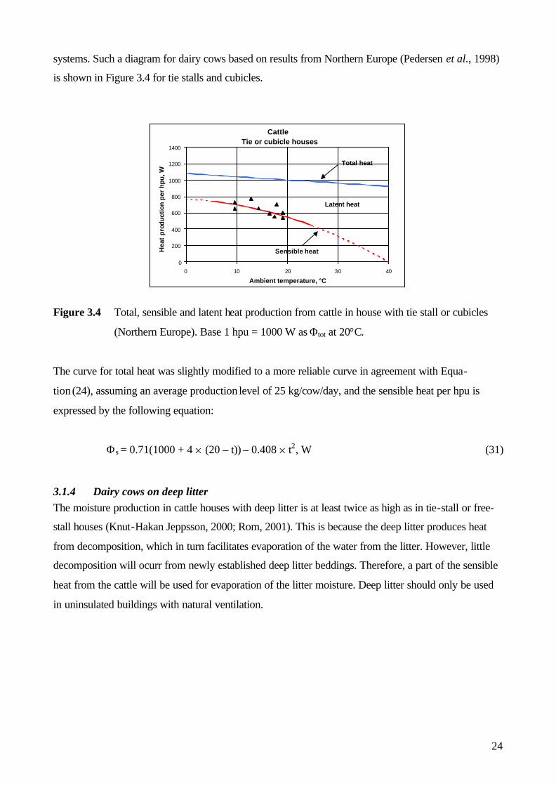
systems. Such a diagram for dairy cows based on results from Northern Europe (Pedersen et al., 1998)
is shown in Figure 3.4 for tie stalls and cubicles.
Figure 3.4 Total, sensible and latent heat production from cattle in house with tie stall or cubicles
(Northern Europe). Base 1 hpu = 1000 W as Φtot at 20°C.
The curve for total heat was slightly modified to a more reliable curve in agreement with Equa-
tion (24), assuming an average production level of 25 kg/cow/day, and the sensible heat per hpu is
expressed by the following equation:
Φs = 0.71(1000 + 4 5 (20 – t)) – 0.408 5 t2, W (31)
3.1.4 Dairy cows on deep litter The moisture production in cattle houses with deep litter is at least twice as high as in tie-stall or free-
stall houses (Knut-Hakan Jeppsson, 2000; Rom, 2001). This is because the deep litter produces heat
from decomposition, which in turn facilitates evaporation of the water from the litter. However, little
decomposition will ocurr from newly established deep litter beddings. Therefore, a part of the sensible
heat from the cattle will be used for evaporation of the litter moisture. Deep litter should only be used
in uninsulated buildings with natural ventilation.
Cattle Tie or cubicle houses
0 200 400 600 800
1000 1200 1400
0 10 20 30 40 Ambient temperature, °C
Hea
t p
rodu
ctio
n pe
r hp
u, W
Sensible heat
Latent heat
Total heat
25
3.2 Pigs
3.2.1 Weaners (See fattening pigs)
3.2.2 Fattening pigs on partly slatted floor
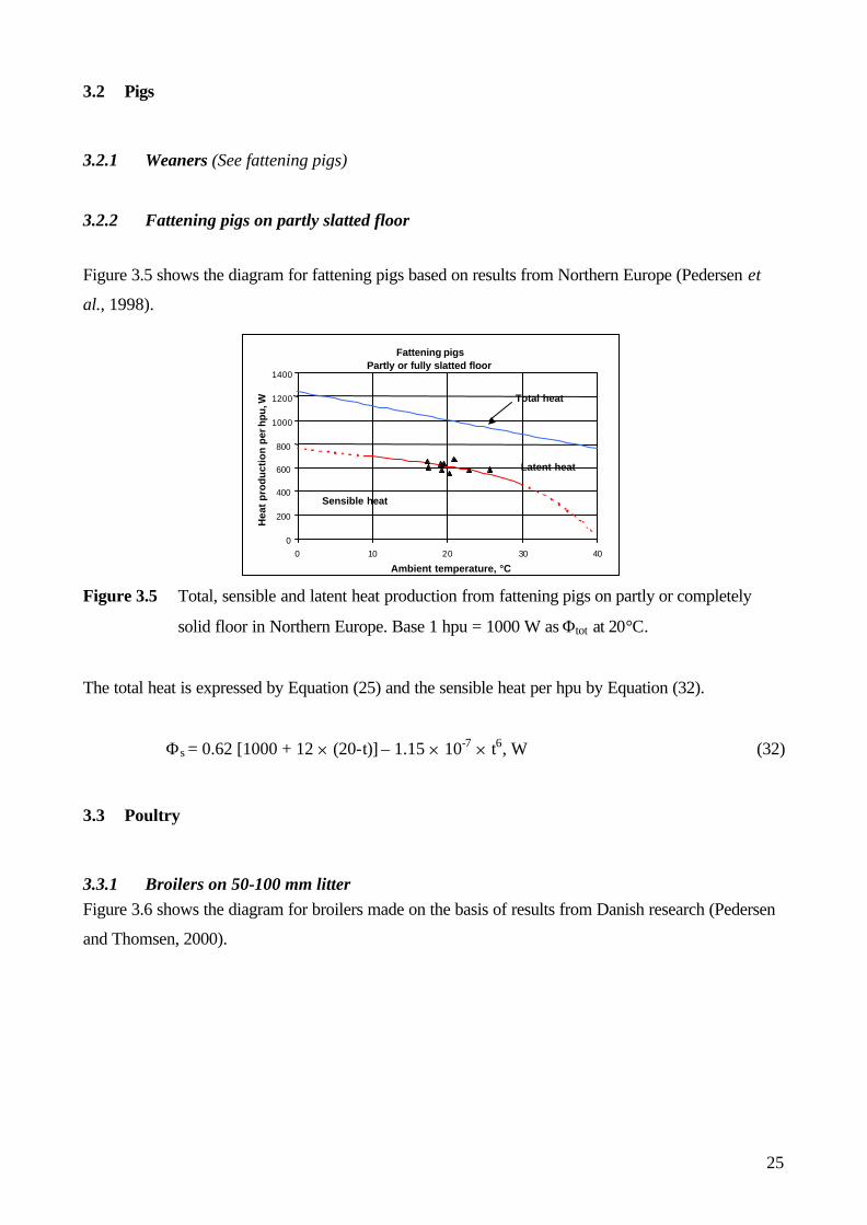
Figure 3.5 shows the diagram for fattening pigs based on results from Northern Europe (Pedersen et
al., 1998).
Figure 3.5 Total, sensible and latent heat production from fattening pigs on partly or completely
solid floor in Northern Europe. Base 1 hpu = 1000 W as Φtot at 20°C.
The total heat is expressed by Equation (25) and the sensible heat per hpu by Equation (32).
Φs = 0.62 [1000 + 12 5 (20-t)] – 1.15 5 10-7 5 t6, W (32)
3.3 Poultry
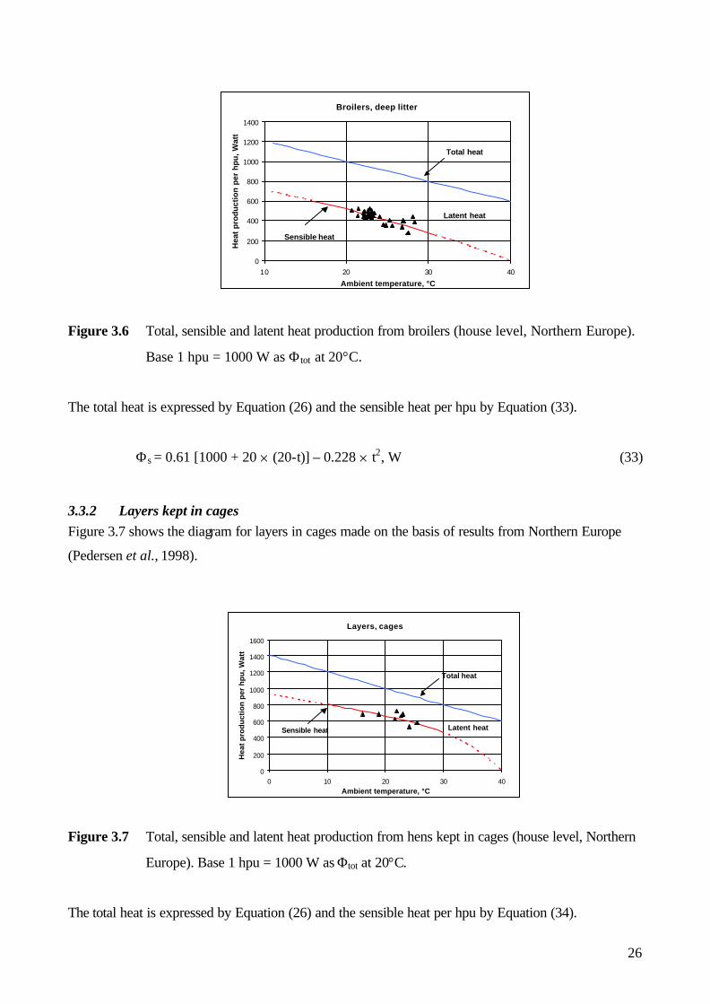
3.3.1 Broilers on 50-100 mm litter Figure 3.6 shows the diagram for broilers made on the basis of results from Danish research (Pedersen
and Thomsen, 2000).
Fattening pigsPartly or fully slatted floor
0
200
400
600
800
1000
1200
1400
0 10 20 30 40
Ambient temperature, °C
Hea
t p
rod
uct
ion
per
hpu
, W
Sensible heat
Latent heat
Total heat
26
Figure 3.6 Total, sensible and latent heat production from broilers (house level, Northern Europe).
Base 1 hpu = 1000 W as Φtot at 20°C.
The total heat is expressed by Equation (26) and the sensible heat per hpu by Equation (33).
Φs = 0.61 [1000 + 20 5 (20-t)] – 0.228 5 t2, W (33)
3.3.2 Layers kept in cages Figure 3.7 shows the diagram for layers in cages made on the basis of results from Northern Europe
(Pedersen et al., 1998).
Figure 3.7 Total, sensible and latent heat production from hens kept in cages (house level, Northern
Europe). Base 1 hpu = 1000 W as Φtot at 20°C.
The total heat is expressed by Equation (26) and the sensible heat per hpu by Equation (34).
Layers, cages
0
200
400
600
800
1000
1200
1400
1600
0 10 20 30 40Ambient temperature, °C
Hea
t p
rod
uct
ion
per
hp
u, W
att
Sensible heat Latent heat
Total heat
Broilers, deep litter
0
200
400
600
800
1000
1200
1400
10 20 30 40
Ambient temperature, °C
Hea
t p
rod
uct
ion
per
hp
u, W
att
Sensible heat
Latent heat
Total heat
27
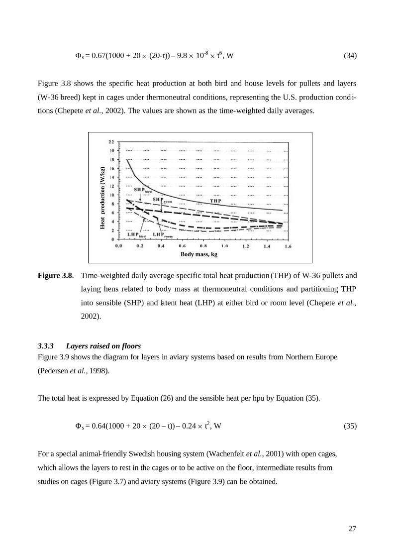
Φs = 0.67(1000 + 20 5 (20-t)) – 9.8 5 10-8 5 t6, W (34)
Figure 3.8 shows the specific heat production at both bird and house levels for pullets and layers
(W-36 breed) kept in cages under thermoneutral conditions, representing the U.S. production cond i-
tions (Chepete et al., 2002). The values are shown as the time-weighted daily averages.
Figure 3.8. Time-weighted daily average specific total heat production (THP) of W-36 pullets and
laying hens related to body mass at thermoneutral conditions and partitioning THP
into sensible (SHP) and latent heat (LHP) at either bird or room level (Chepete et al.,
2002).
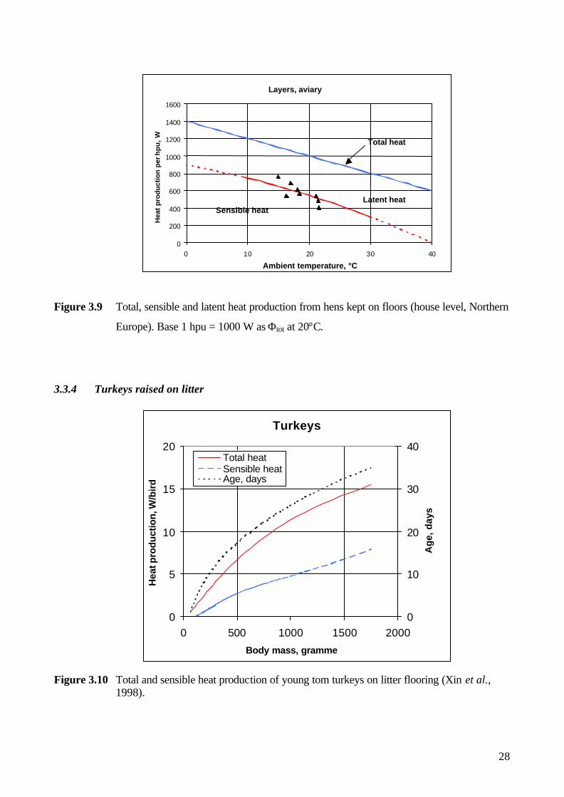
3.3.3 Layers raised on floors Figure 3.9 shows the diagram for layers in aviary systems based on results from Northern Europe
(Pedersen et al., 1998).
The total heat is expressed by Equation (26) and the sensible heat per hpu by Equation (35).
Φs = 0.64(1000 + 20 5 (20 – t)) – 0.24 5 t2, W (35)
For a special animal- friendly Swedish housing system (Wachenfelt et al., 2001) with open cages,
which allows the layers to rest in the cages or to be active on the floor, intermediate results from
studies on cages (Figure 3.7) and aviary systems (Figure 3.9) can be obtained.
Hea
t pr
oduc
tion
(W/k
g)
Body mass, kg
28
Figure 3.9 Total, sensible and latent heat production from hens kept on floors (house level, Northern
Europe). Base 1 hpu = 1000 W as Φtot at 20°C.
3.3.4 Turkeys raised on litter
Figure 3.10 Total and sensible heat production of young tom turkeys on litter flooring (Xin et al., 1998).
Layers, aviary
0
200
400
600
800
1000
1200
1400
1600
0 10 20 30 40
Ambient temperature, °C
Hea
t p
rod
uct
ion
per
hp
u,
W
Sensible heatLatent heat
Total heat
Turkeys
0
5
10
15
20
0 500 1000 1500 2000
Body mass, gramme
Hea
t pro
duct
ion,
W/b
ird
0
10
20
30
40
Ag
e, d
ays
Total heatSensible heatAge, days
29
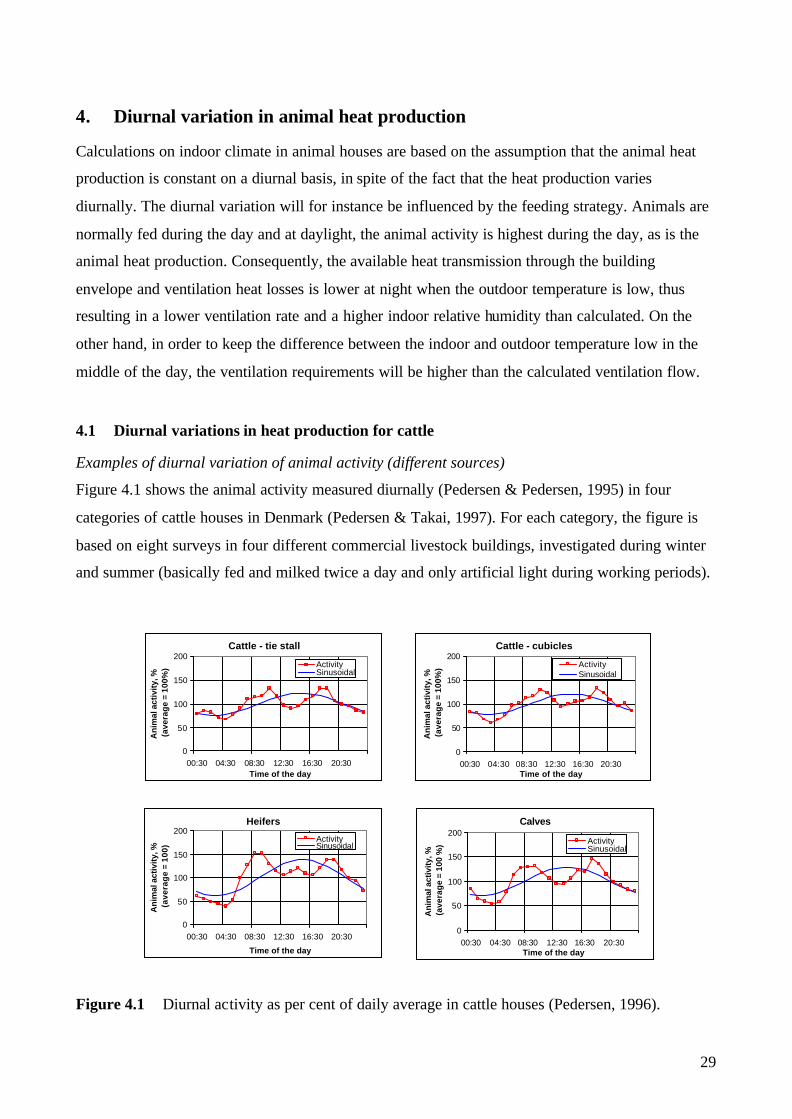
4. Diurnal variation in animal heat production
Calculations on indoor climate in animal houses are based on the assumption that the animal heat
production is constant on a diurnal basis, in spite of the fact that the heat production varies
diurnally. The diurnal variation will for instance be influenced by the feeding strategy. Animals are
normally fed during the day and at daylight, the animal activity is highest during the day, as is the
animal heat production. Consequently, the available heat transmission through the building
envelope and ventilation heat losses is lower at night when the outdoor temperature is low, thus
resulting in a lower ventilation rate and a higher indoor relative humidity than calculated. On the
other hand, in order to keep the difference between the indoor and outdoor temperature low in the
middle of the day, the ventilation requirements will be higher than the calculated ventilation flow.
4.1 Diurnal variations in heat production for cattle
Examples of diurnal variation of animal activity (different sources)
Figure 4.1 shows the animal activity measured diurnally (Pedersen & Pedersen, 1995) in four
categories of cattle houses in Denmark (Pedersen & Takai, 1997). For each category, the figure is
based on eight surveys in four different commercial livestock buildings, investigated during winter
and summer (basically fed and milked twice a day and only artificial light during working periods).
Figure 4.1 Diurnal activity as per cent of daily average in cattle houses (Pedersen, 1996).
Cattle - cubicles
0
50
100
150
200
00:30 04:30 08:30 12:30 16:30 20:30Time of the day
An
imal
act
ivity
, %(a
vera
ge
= 10
0%) Activity
Sinusoidal
Cattle - tie stall
0
50
100
150
200
00:30 04:30 08:30 12:30 16:30 20:30Time of the day
An
imal
act
ivity
, %(a
vera
ge
= 10
0%) Activity
Sinusoidal
Heifers
0
50
100
150
200
00:30 04:30 08:30 12:30 16:30 20:30
Time of the day
An
imal
act
ivity
, %(a
vera
ge
= 1
00)
ActivitySinusoidal
Calves
0
50
100
150
200
00:30 04:30 08:30 12:30 16:30 20:30Time of the day
An
imal
act
ivity
, %(a
vera
ge
= 10
0 %
) ActivitySinusoidal
30
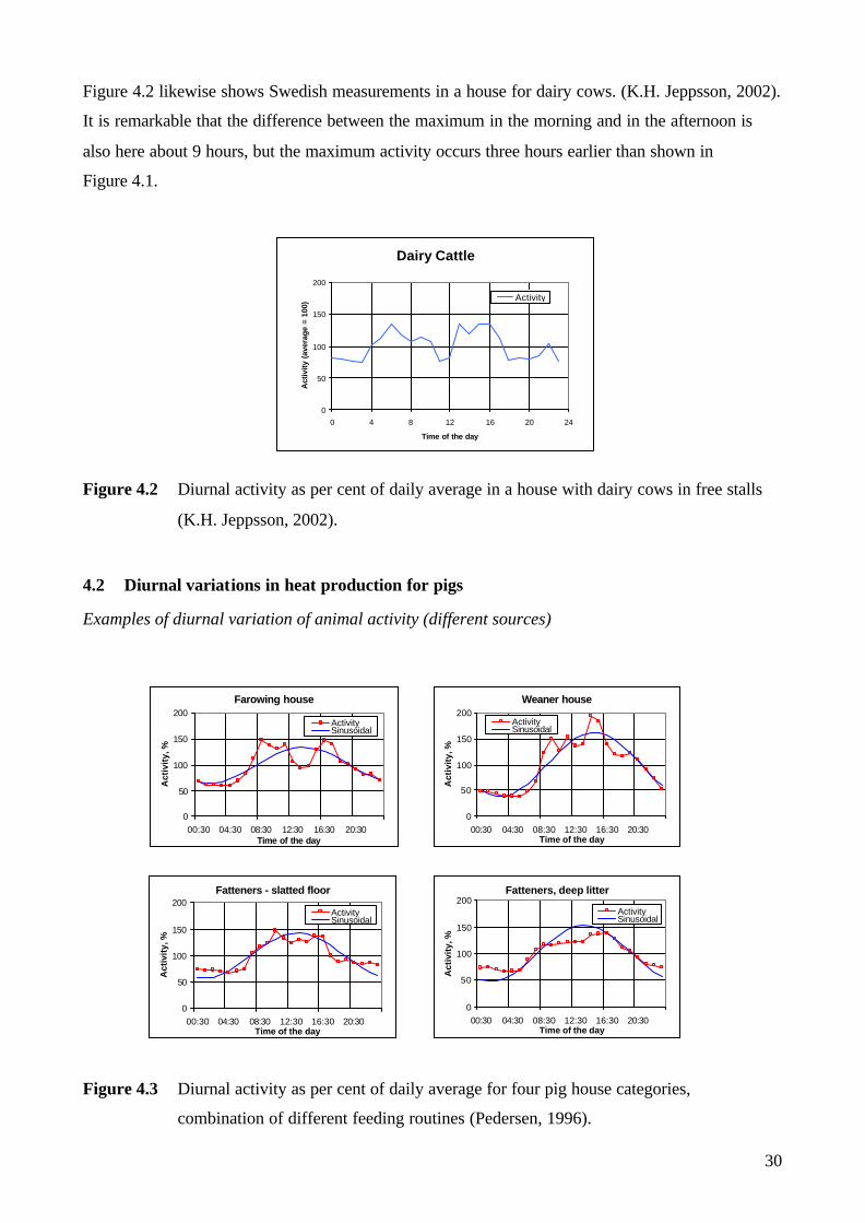
Figure 4.2 likewise shows Swedish measurements in a house for dairy cows. (K.H. Jeppsson, 2002).
It is remarkable that the difference between the maximum in the morning and in the afternoon is
also here about 9 hours, but the maximum activity occurs three hours earlier than shown in
Figure 4.1.
Figure 4.2 Diurnal activity as per cent of daily average in a house with dairy cows in free stalls
(K.H. Jeppsson, 2002).
4.2 Diurnal variations in heat production for pigs
Examples of diurnal variation of animal activity (different sources)
Figure 4.3 Diurnal activity as per cent of daily average for four pig house categories,
combination of different feeding routines (Pedersen, 1996).
Dairy Cattle
0
50
100
150
200
0 4 8 12 16 20 24
Time of the day
Act
ivity
(av
erag
e =
100)
Activity
Weaner house
0
50
100
150
200
00:30 04:30 08:30 12:30 16:30 20:30Time of the day
Act
ivit
y, %
ActivitySinusoidal
Fatteners - slatted floor
0
50
100
150
200
00:30 04:30 08:30 12:30 16:30 20:30Time of the day
Act
ivit
y, %
ActivitySinusoidal
Fatteners, deep litter
0
50
100
150
200
00:30 04:30 08:30 12:30 16:30 20:30Time of the day
Act
ivit
y, %
ActivitySinusoidal
Farowing house
0
50
100
150
200
00:30 04:30 08:30 12:30 16:30 20:30Time of the day
Act
ivit
y, %
ActivitySinusoidal
31
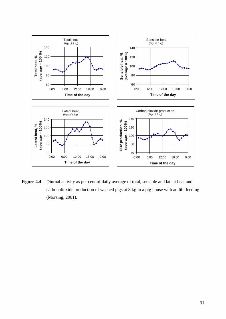
Figure 4.4 Diurnal activity as per cent of daily average of total, sensible and latent heat and
carbon dioxide production of weaned pigs at 8 kg in a pig house with ad lib. feeding
(Morsing, 2001).
Total heat(Pigs of 8 kg)
60
80
100
120
140
0:00 6:00 12:00 18:00 0:00
Time of the day
To
tal h
eat,
%(a
vera
ge
= 10
0 %
)Sensible heat
(Pigs of 8 kg)
60
80
100
120
140
0:00 6:00 12:00 18:00 0:00
Time of the day
Sen
sib
le h
eat,
%(a
vera
ge
= 10
0%)
Latent heat(Pigs of 8 kg)
60
80
100
120
140
0:00 6:00 12:00 18:00 0:00
Time of the day
Lat
ent h
eat,
%(a
vera
ge
= 10
0%)
Carbon dioxide production(Pigs of 8 kg)
60
80
100
120
140
0:00 6:00 12:00 18:00 0:00
Time of the day
CO
2 p
rod
uct
ion
, %(a
vera
ge
= 10
0%)
32
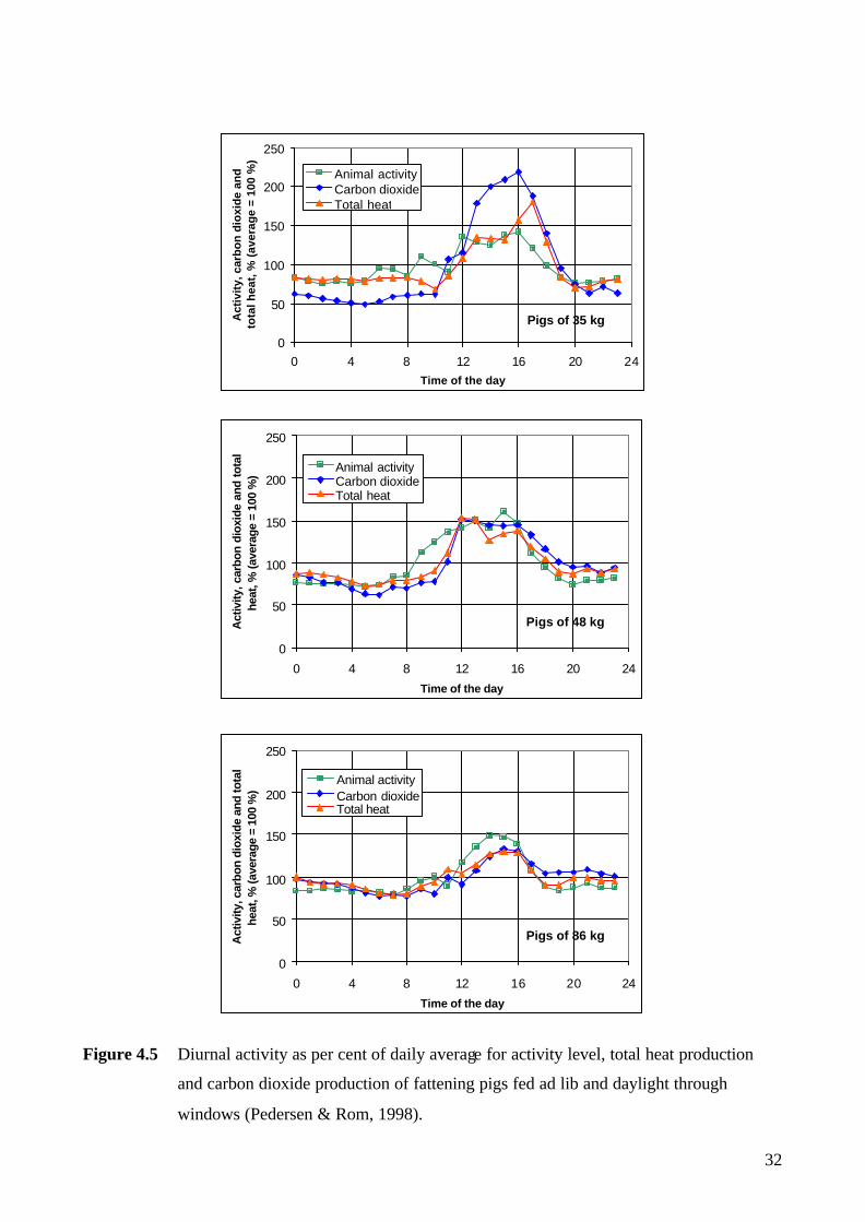
Figure 4.5 Diurnal activity as per cent of daily average for activity level, total heat production
and carbon dioxide production of fattening pigs fed ad lib and daylight through
windows (Pedersen & Rom, 1998).
Pigs of 35 kg
0
50
100
150
200
250
0 4 8 12 16 20 24Time of the day
Act
ivit
y, c
arb
on
dio
xid
e an
d
tota
l hea
t, %
(av
erag
e =
100
%)
Animal activityCarbon dioxideTotal heat
Pigs of 48 kg
0
50
100
150
200
250
0 4 8 12 16 20 24
Time of the day
Act
ivity
, car
bon
diox
ide
and
tota
l he
at, %
(ave
rage
= 1
00 %
)
Animal activityCarbon dioxideTotal heat
Pigs of 86 kg
0
50
100
150
200
250
0 4 8 12 16 20 24
Time of the day
Act
ivity
, car
bon
diox
ide
and
tota
l he
at, %
(ave
rage
= 1
00 %
)
Animal activityCarbon dioxideTotal heat
33
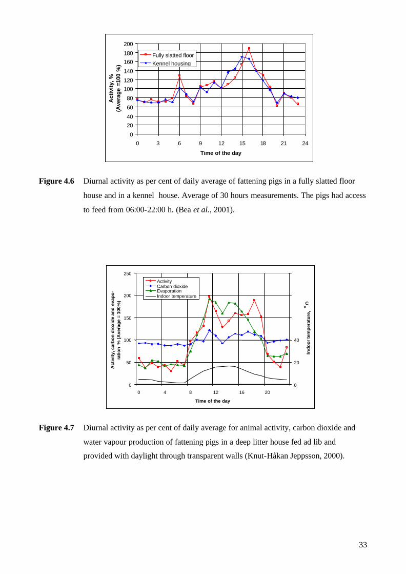
Figure 4.6 Diurnal activity as per cent of daily average of fattening pigs in a fully slatted floor
house and in a kennel house. Average of 30 hours measurements. The pigs had access
to feed from 06:00-22:00 h. (Bea et al., 2001).
Figure 4.7 Diurnal activity as per cent of daily average for animal activity, carbon dioxide and
water vapour production of fattening pigs in a deep litter house fed ad lib and
provided with daylight through transparent walls (Knut-Håkan Jeppsson, 2000).
0
20
40
60
80
100
120
140
160
180
200
0 3 6 9 12 15 18 21 24
Time of the day
Act
ivit
y, %
(Ave
rage
=10
0 %
)
Fully slatted floorKennel housing
0
50
100
150
200
250
0 4 8 12 16 20
Time of the day
Act
ivity
, car
bon
dio
xid
e an
d e
vap
o-
rati
on
% (A
vera
ge
= 10
0%)
0
20
40
Indo
or te
mpe
ratu
re,
oC
ActivityCarbon dioxideEvaporationIndoor temperature
34
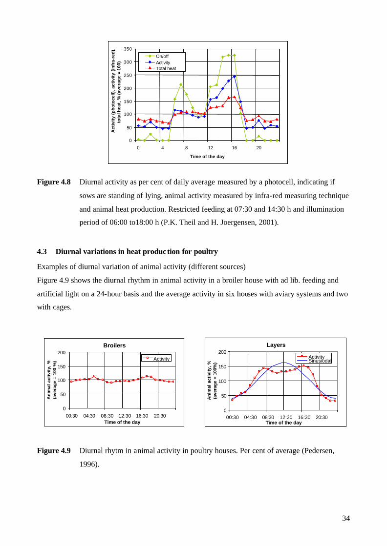
Figure 4.8 Diurnal activity as per cent of daily average measured by a photocell, indicating if
sows are standing of lying, animal activity measured by infra-red measuring technique
and animal heat production. Restricted feeding at 07:30 and 14:30 h and illumination
period of 06:00 to18:00 h (P.K. Theil and H. Joergensen, 2001).
4.3 Diurnal variations in heat production for poultry
Examples of diurnal variation of animal activity (different sources)
Figure 4.9 shows the diurnal rhythm in animal activity in a broiler house with ad lib. feeding and
artificial light on a 24-hour basis and the average activity in six houses with aviary systems and two
with cages.
Figure 4.9 Diurnal rhytm in animal activity in poultry houses. Per cent of average (Pedersen,
1996).
0
50
100
150
200
250
300
350
0 4 8 12 16 20
Time of the day
Act
ivity
(p
ho
toce
ll), a
ctiv
ity (
infr
a-re
d),
tota
l hea
t, %
(ave
rag
e =
100)
On/offActivityTotal heat
Broilers
0
50
100
150
200
00:30 04:30 08:30 12:30 16:30 20:30Time of the day
An
imal
act
ivit
y, %
(a
vera
ge =
100
%) Activity
Layers
0
50
100
150
200
00:30 04:30 08:30 12:30 16:30 20:30Time of the day
An
imal
act
ivit
y, %
(a
vera
ge =
100
%)
ActivitySinusiodal
35
Broilers
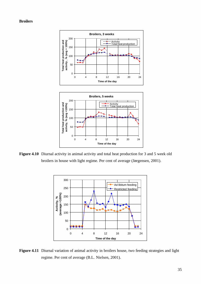
Figure 4.10 Diurnal activity in animal activity and total heat production for 3 and 5 week old
broilers in house with light regime. Per cent of average (Jørgensen, 2001).
Figure 4.11 Diurnal variation of animal activity in broilers house, two feeding strategies and light
regime. Per cent of average (B.L. Nielsen, 2001).
Broilers, 5 weeks
0
50
100
150
200
0 4 8 12 16 20 24
Time of the day
To
tal h
eat
pro
du
ctio
n a
nd
ac
tivi
ty, %
(av
g =
100%
) ActivityTotal heat production
Broilers, 3 weeks
0
50
100
150
200
0 4 8 12 16 20 24
Time of the day
To
tal h
eat
pro
du
ctio
n a
nd
ac
tivi
ty ,
% (
avg
= 1
00%
)
ActivityTotal heat production
0
50
100
150
200
250
300
0 4 8 12 16 20 24
Time of the day
Act
ivit
y, %
(ave
rag
e =1
00%
)
Ad libitum feeding
Restricted feeding
36
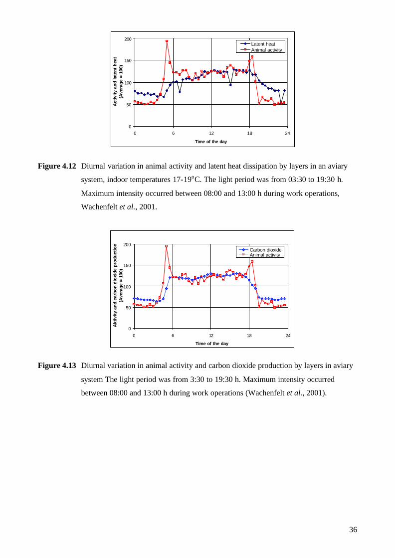
Figure 4.12 Diurnal variation in animal activity and latent heat dissipation by layers in an aviary
system, indoor temperatures 17-19oC. The light period was from 03:30 to 19:30 h.
Maximum intensity occurred between 08:00 and 13:00 h during work operations,
Wachenfelt et al., 2001.
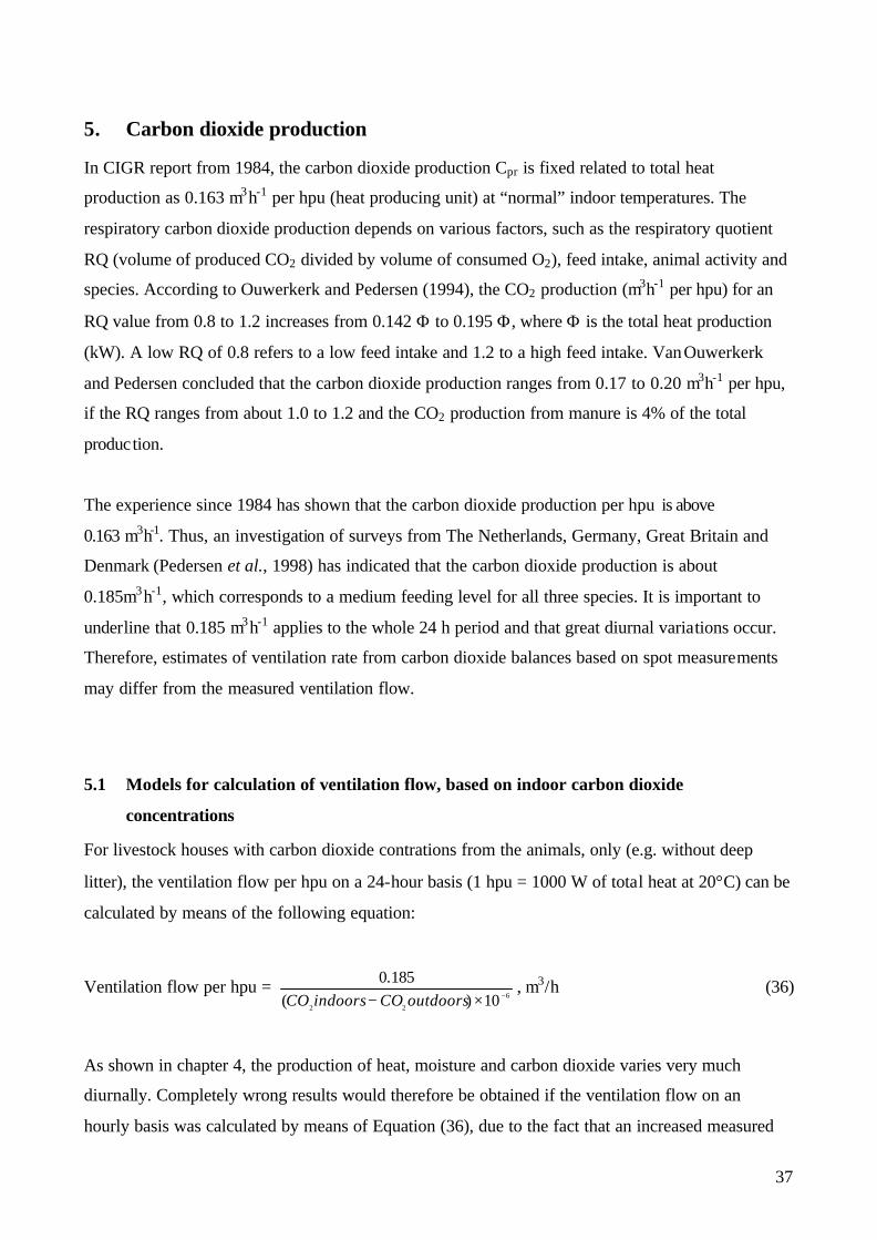
Figure 4.13 Diurnal variation in animal activity and carbon dioxide production by layers in aviary
system The light period was from 3:30 to 19:30 h. Maximum intensity occurred
between 08:00 and 13:00 h during work operations (Wachenfelt et al., 2001).
0
50
100
150
200
0 6 12 18 24
Time of the day
Act
ivity
and
late
nt h
eat
(Ave
rage
= 1
00)
Latent heatAnimal activity
0
50
100
150
200
0 6 12 18 24
Time of the day
Akt
ivit
y an
d c
arb
on
dio
xid
e p
rod
uct
ion
(Ave
rage
= 1
00)
Carbon dioxideAnimal activity
37
5. Carbon dioxide production
In CIGR report from 1984, the carbon dioxide production Cpr is fixed related to total heat
production as 0.163 m3h-1 per hpu (heat producing unit) at “normal” indoor temperatures. The
respiratory carbon dioxide production depends on various factors, such as the respiratory quotient
RQ (volume of produced CO2 divided by volume of consumed O2), feed intake, animal activity and
species. According to Ouwerkerk and Pedersen (1994), the CO2 production (m3h-1 per hpu) for an
RQ value from 0.8 to 1.2 increases from 0.142 Φ to 0.195 Φ, where Φ is the total heat production
(kW). A low RQ of 0.8 refers to a low feed intake and 1.2 to a high feed intake. Van Ouwerkerk
and Pedersen concluded that the carbon dioxide production ranges from 0.17 to 0.20 m3h-1 per hpu,
if the RQ ranges from about 1.0 to 1.2 and the CO2 production from manure is 4% of the total
production.
The experience since 1984 has shown that the carbon dioxide production per hpu is above
0.163 m3h-1. Thus, an investigation of surveys from The Netherlands, Germany, Great Britain and
Denmark (Pedersen et al., 1998) has indicated that the carbon dioxide production is about
0.185m3h-1, which corresponds to a medium feeding level for all three species. It is important to
underline that 0.185 m3h-1 applies to the whole 24 h period and that great diurnal variations occur.
Therefore, estimates of ventilation rate from carbon dioxide balances based on spot measurements
may differ from the measured ventilation flow.
5.1 Models for calculation of ventilation flow, based on indoor carbon dioxide
concentrations
For livestock houses with carbon dioxide contrations from the animals, only (e.g. without deep
litter), the ventilation flow per hpu on a 24-hour basis (1 hpu = 1000 W of total heat at 20°C) can be
calculated by means of the following equation:
Ventilation flow per hpu = 6
22 10)(185.0
−×− outdoorsCOindoorsCO, m3/h (36)
As shown in chapter 4, the production of heat, moisture and carbon dioxide varies very much
diurnally. Completely wrong results would therefore be obtained if the ventilation flow on an
hourly basis was calculated by means of Equation (36), due to the fact that an increased measured
38
carbon dioxide concentration will lead to a lower calculated ventilation flow if the value
0.185 m3h-1 is kept as a fixed value. On an hourly basis, the carbon dioxide production would have
to be adjusted for animal activity. If the animal activity is measured, the adjustment of the carbon
dioxide concentration can be made directly. Otherwise, the adjustment on an hourly basis could be
done indirectly by means of the following equation:
Ventilation flow per hpu = 6
22 10)()(185.0−×−
×outdoorsCOindoorsCO
activity animal relative , m3/h (37)
Two main models for activity (the dromedary model and the camel model) could be used.
Sinusoidal dromedary model for diurnal variation in animal activity
The animal activity can be approximated by the following sinusoidal equation:
A = 1-a 5 sin[(2 5 π/24) 5 (h + 6 - hmin)] (38)
where:
A = relative animal activity
a = constant (expressing the amplitude with respect to the constant 1)
hmin = time of the day with minimum activity (hours after midnight)
The parameters for Equation 38 for cattle, pigs and poultry have been calculated for livestock
buildings in Denmark, as shown in Table 5.1.
Table 5.1. Parameters for Equation 34, based on 10 diurnal measurements in each of
10 Danish livestock buildings
Type of animals a Time of the day with minimum activity
Dairy cows, tie stall 0.23 2.2 (02:10) Dairy cows, cubicles 0.22 2.9 (02:55) Heifers 0.38 3.1 (03:05) Calves 0.29 2.0 (02:00) Lactating sows 0.35 1.8 (01:50) Weaners 0.63 2.9 (02:55) Fattening pigs, partly slatted floor 0.43 1.3 (01:20) Fattening pigs, deep litter 0.53 1.7 (01:40) Layers 0.61 -0.1 (23:55) Broilers (permanent light and ad lib. feeding) 0.08 Not defined
The table shows that in most cases, the minimum activity occurs at about 2:00 h, and that the
maximum and minimum activity differs from 8 to 63% of the diurnal average. Except for broilers
39
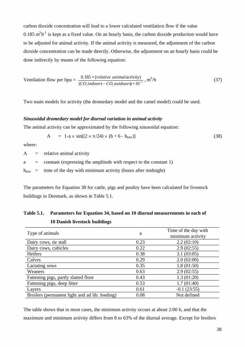
with permanent light and access to feed, the diurnal variations will in all cases be above 20%
(a > 0.2, see Table 5.1). On the basis of different experiments described in chapter 4, it is possible
to make a general correction of total and latent heat in respect to the time of the day, as shown in
Figure 5.1 for a = 0.2.
Figure 5.1 Standard correction of animal heat production due to diurnal variation (dromedary
model).
Sinusoidal camel model for diurnal variation in animal activity
For animal houses with typically two maximums of animal activity during the day, a more
sophisticated approach by a combination of two equations can be used. Equation (39) is for the
activity in the daytime, and Equation (40) for the activity during the night:
Daytime: A = 1 - a 5 sin [(2 5 p/24) 5 (h + 6 -hmin)] – b 5 sin [(2 5 p/11) 5 (h –11.3)] (39)
Nighttime: A = 1- a 5 sin [(2 5 p/24) 5 (h + 6 -hmin)] (40)
where:
A = animal activity
a = constant expressing the amplitude relative to 1 (06:00-22:00 h)
b = constant expressing the amplitude relative to 1 (22:00-06:00 h).
The numbers hmin and -11.3 in Equations (39) and (40) are the adjustment of the time of the day
with maximum activity. The maximum activity in the afternoon is set to occur 11 hours later than in
the morning. For a = 0.2, and b = 0.15, Figure 5.2 shows an example.
Activity
0.0
0.5
1.0
1.5
0 4 8 12 16 20 24
Time of the day
Act
ivity
fact
or
40
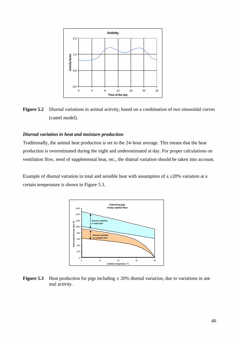
Figure 5.2 Diurnal variations in animal activity, based on a combination of two sinusoidal curves
(camel model).
Diurnal variation in heat and moisture production
Traditionally, the animal heat production is set to the 24-hour average. This means that the heat
production is overestimated during the night and underestimated at day. For proper calculations on
ventilation flow, need of supplemental heat, etc., the diurnal variation should be taken into account.
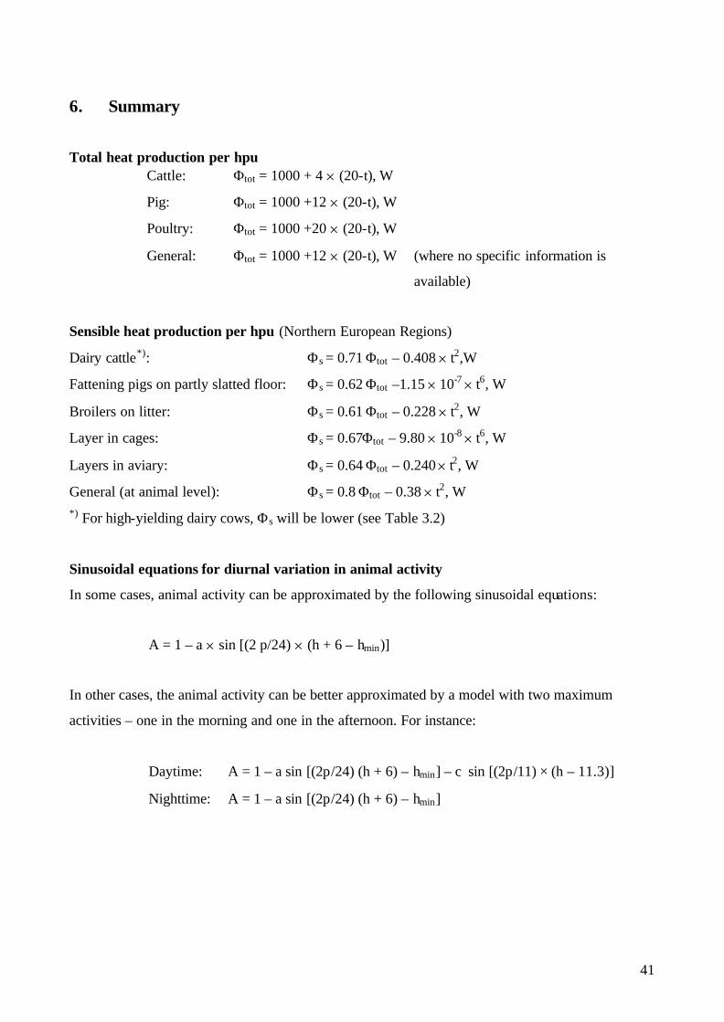
Example of diurnal variation in total and sensible heat with assumption of a ±20% variation at a
certain temperature is shown in Figure 5.3.
Figure 5.3 Heat production for pigs including ± 20% diurnal variation, due to variations in ani-mal activity.
Activity
0.0
0.5
1.0
1.5
0 4 8 12 16 20 24
Time of the day
Act
ivity
fact
or
Fattening pigs Partly slatted floor
0
200
400
600
800
1000
1200
1400
1600
0 10 20 30 40
Ambient temperture, °C
Hea
t pro
duct
ion
per
hp
u, W
Diurnal variationin sensible heat
Diurnal variationin total heat
41
6. Summary
Total heat production per hpu Cattle: Φtot = 1000 + 4 5 (20-t), W
Pig: Φtot = 1000 +12 5 (20-t), W
Poultry: Φtot = 1000 +20 5 (20-t), W
General: Φtot = 1000 +12 5 (20-t), W (where no specific information is
available)
Sensible heat production per hpu (Northern European Regions)
Dairy cattle*): Φs = 0.71 Φtot – 0.408 5 t2,W
Fattening pigs on partly slatted floor: Φs = 0.62 Φtot –1.15 5 10-7 5 t6, W
Broilers on litter: Φs = 0.61 Φtot – 0.228 5 t2, W
Layer in cages: Φs = 0.67Φtot – 9.80 5 10-8 5 t6, W
Layers in aviary: Φs = 0.64 Φtot – 0.240 5 t2, W
General (at animal level): Φs = 0.8 Φtot – 0.38 5 t2, W *) For high-yielding dairy cows, Φs will be lower (see Table 3.2)
Sinusoidal equations for diurnal variation in animal activity
In some cases, animal activity can be approximated by the following sinusoidal equations:
A = 1 – a 5 sin [(2 p/24) 5 (h + 6 – hmin)]
In other cases, the animal activity can be better approximated by a model with two maximum
activities – one in the morning and one in the afternoon. For instance:
Daytime: A = 1 – a⋅sin [(2p/24) (h + 6) – hmin] – c⋅ sin [(2p/11) × (h – 11.3)]
Nighttime: A = 1 – a⋅sin [(2p/24) (h + 6) – hmin]
42
7. References
ASHRAE Handbook, Standard. 2001a. American Society of Heating, Refrigerating, and Air-
conditioning Engineers: Atlanta, GA, USA.
ASHRAE Handbook, Fundamentals. 2001b. American Society of Heating, Refrigerating, and Air-
conditioning Engineers: Atlanta, GA, USA.
Bea, W., Hartung,E., Jungbluth, T. & Troxler, J. 2001. Ethological Evaluation of an Alternative
Housing System for Fattening Pigs. Proceedings of the International CIGR symposium on
Animal Welfare Considerations in Livestock Housing Systems, Szklarska Poreba, Poland:
111-118.
Chepete, H. J. and H. Xin. 2002. Heat and moisture production of poultry and their housing systems:
Literature review. Transactions of the ASHRAE 85(2).
Chepete, H. J., H. Xin, M. C. Puma, and R. S. Gates. 2002. Heat and moisture production of poultry
and their housing systems: Pullets and layers. Transactions of the ASHRAE (in review).
CIGR report, 1984. Climatization of Animal Houses. Report of working group. Scottish Farm
Building Investigation Unit. Craibstone, Aberdeen, Scotland.
CIGR report, 1992 Climatization of Animal Houses. Second report of working group. Faculty of
Agricultural Sciences, State University of Ghent, Belgium.
CIGR Handbook, 1999. CIGR Handbook of Agricultural Engineering, Volume II. Animal
Production & Aquacultural Engineering. Published by American Society of Agricultural
Engineers.
Chwalibog A, Eggum B O, 1989. Effect of temperature on performance, heat production,
evaporative heat loss and body composition in chickens. Archiv für Geflügelkunde 53(4):
179-184.
Collin, A., Milgen, J. van, Dubois, S. & Noblet, J. 2001. Effect of high temperature and feeding
level on energy utilization in piglets. J.Anim. Sci. 79: 1849-1857.
Ehrlemark, A.G. & Sällvik, K. 1996. A Model of Heat and Moisture Dissipation from Cattle Based
on Thermal Properties. Transactions of the ASAE, Vol. 39 (1); 187.
Elnif, J, 2001. Heat production for mink. The Royal Veterinary and Agricultural University
(Unpublished)
Hutchinson J C A, 1954. Evaporative cooling in fowls, Journal of Agricultural Science, Cambridge,
(45):48-59.
Jeppsson, K.H., 2000. Aerial environment in uninsulated livestock buildings, Agraria 245 (Thesis)
Swedish University of Agricultural Sciences.
Joergensen, H., 2001. Broiler activity. Danish Institute of Agricultural Sciences (unpublished).
43
Morsing, S. 2001. Heat production for weaned pigs. Danish Institute of Agricultural Sciences
(unpublished).
Nielsen, B., L. 2001. Broiler activity. Danish Institute of Agricultural Sciences (unpublished).
Ota, H., Whitehead, J. A., & Davey R.J., 1982. Heat production of male and female piglets.
Proceedings of Second International Livestock Environment Symposium, SP 03-82, ASAE,
St. Joseph, MI.
Pedersen, J., Chwalibog, A., & Eggum, B.O. 1985. Measurement of broiler latent and sensible heat
production (in Danish). Danish Institute of Animal Science. Report No. 573.
Pedersen, S & Pedersen, C.B. 1995. Animal Activity Measured by Infrared Detectors, Journal of
Agricultural Engineering Research, (61): 239-246.
Pedersen, S., Takai, H., Johnsen, J.O., Metz, J.H.M., Groot Koerkamp, P.W.G., Uenk, G.H.,
Phillips, V.R., Holden, M.R., Sneath, R.W., Short, J.L., White, R.P., Hartung, J., Seedorf, J.,
Schroeder, M., Linkert, K.H. & Wathes, C.M., 1998. A Comparison of Three Balance
Methods for Calculating Ventilation Flow Rates in Livestock Buildings. Journal of
Agricultural Engineering Research. Volume 70, Number 1, Special Issues: 25-37.
Pedersen, S. & Takai, H. 1997. Diurnal Variation in Animal Heat Production in Relation to Animal
Activity. Paper for presentation at the ILES V in Minnesota
Pedersen, S., 1994. Behaviour of Dairy cows Recorded by Activity Monitoring System. Third
International Dairy Housing Conference, 2-5 February, Florida. ASAE Publication 02-94:
410-414.
Pedersen, S., 1996. Døgnvariationer i dyrenes aktivitet i kvæg-, svine og fjerkræstalde. Delresultater
fra EU-projekt PL 900703. Diurnal variations in animal activity in buildings for cattle, pigs
and poultry. Subresults from EU-project PL 900703. (in Danish). National Institute of Animal
Science, Denmark, Internal report No. 66, 33 pp.
Pedersen, S., 1996. Chapter 2. Production of heat and moisture. CIGR Working Group on
"Fundamentals of farm animal environment and energy consumption. Working Group Report.
(SIG 14. Air quality in animal houses), Madrid.
Pedersen, S. & Takai, H., 1997. Diurnal Variation in Animal Heat Production in Relation to Animal
Activity. Fifth International Livestock Environment Symposium, Minnesota, May 29-31.
Proceedings, vo lume 2:664-671.
Pedersen, S., Phillips, V.R., Seedorf, J. & Koerkamp, P.W.G.G., 1996. A comparison of three
different balance methods for calculating the ventilation flow rate in Northern European
livestock buildings. AgEng96 Madrid. International Conference on Agricultural Engineering,
Volume 1: Pages 413-414 and Paper No. 96B-049.
44
Pedersen, S. & Rom, H.B., 1998. Diurnal Variation in Heat Production from Pigs in Relation to
Animal Activity. AgEng Oslo98. Paper 98-B-025. Published in 1999 on a CD as: pdf\b\98-B-
024.pdf.
Pedersen, S., Takai, H., Johnsen, J.O., Metz, J.H.M., Groot Koerkamp, P.W.G., Uenk, G.H.,
Phillips, V.R., Holden, M.R., Sneath, R.W., Short, J.L., White, R.P., Hartung, J., Seedorf, J.,
Schroeder, M., Linkert, K.H. & Wathes, C.M. 1998. A Comparison of Three Balance
Methods for Calculating Ventilation Flow Rates in Livestock Buildings. Journal of
Agricultural Engineering Research. Volume 70, Number 1, Special Issues: 25-37.
Pedersen, S. & Thomsen, M.G., 2000. Heat and Moisture Production for Broilers on Straw
Bedding. Journal of Agricultural Engineering Research, 75, 177-187.
Quiniou, N., Noblet, J., Milgen, J. van, & Dubois, S. 2001. Modelling heat and energy balance in
group-housed growing pigs exposed to low or high ambient temperatures. British Journal of
Nutrition 85: 97-106.
Rom, H.B., 2001. Moisture production in deep litter house for cattle. Danish Institute of
Agricultural Sciences (Unpublished).
Sällvik, K & Pedersen, S., 1999. Animal Heat and Moisture Production, in CIGR Handbook of
Agricultural Engineering. Volume II. Animal Production & Aquacultural Engineering. Part I
Livestock Housing and Environment - Chapter 2.2. (Editor, El Houssine Bartali). Published
by ASAE: 41-54.
Strøm J.S., 1978. Heat loss from cattle, swine and poultry as basis for design of environmental
control systems in livestock buildings (in Danish). SBI-Landbrugsbyggeri 55, Danish
Building Research Institute, Denmark.
Swedish Standard SS 951050, 1992.
Theil, P.K., & Joergensen, H. 2001. Animal activity and heat production. Danish Institute of
Agricultural Sciences (unpublished).
Tzschentke, B., Nichelmann, M. & Postel, P. 1996. Effects of ambient temperature, age and wind
speed on the thermal balance of layer-strain fowls. British Poultry Science, 37: 501-520.
Van Caenegem, L. 2002. Carbon dioxide concentrations in house for dairy cattle. Swiss Federal
Research Station for Agricultural Economics and Engineering (Unpublished).
van Ouwerkerk, E N J & Pedersen, S. 1994. Application of the carbon dioxide mass balance method
to evaluate ventilation rates in livestock buildings. XII CIGR World Congress on Agricultural
Engineering, Milan. Proceedings, Volume 1, 516-529.
Wachenfelt, E.V., Pedersen, S. & Gustafsson, G. 2001. Release of heat, moisture and carbon
dioxide in an aviary system for laying hens. British Poultry Science (2001) 42: 171-179.
45
Wathes, C M. 1981. Insulation of animal houses. In: Environmental Aspects of Housing for Animal
Production. Eds. J.A. Clark, Butterworths, London: 379-412.
Xin, H., I. L. Berry, G. T. Tabler, and T. A. Costello. 2001. Heat and moisture production of poultry
and their housing system: Broilers. Transactions of the ASAE 44(6): 1853-1859.
Xin, H., Chepete, H.J., Shao, J., & Sell, J.L. 1998. Heat and moisture production and minimum
ventilation requirements of tom turkeys during brooding-growing period. Transactions of the
ASAE Vol. 41(5): 1489-1498.

ISBN 87-88976-60-2