Embed Size (px)
Citation preview
Health Investment over the Life-Cycle∗
Timothy J. Halliday†, Hui He‡, Lei Ning§, and Hao Zhang¶
August 27, 2016
∗We thank Carl Bonham, Michele Boldrin, Toni Braun, Kaiji Chen, Sumner La Croix, KevinHuang, Selo Imrohoroglu, Sagiri Kitao, Nobu Kiyotaki, Dirk Krueger, Zheng Liu, Andy Mason,Makoto Nakajima, Michael Palumbo, Richard Rogerson, Richard Suen, Motohiro Yogo, Kai Zhao,seminar participants at the Chinese University of Hong Kong, the Federal Reserve Board, GeorgeWashington University, Hong Kong University of Science and Technology, Peking University, Shang-hai University of Finance and Economics, University of Hawai’i at Manoa, Utah State University,and conference participants at the 2009 Midwest Macroeconomics Meeting, 2009 QSPS SummerWorkshop, 2009 Western Economic Association International (WEAI) Meeting, 15th InternationalConference on Computing in Economics and Finance in Sydney, 2010 Tsinghua Workshop inMacroeconomics, and 2010 SED Annual Meeting for helpful feedback. We thank Jesus Fernandez-Villaverde for providing us consumption data. Financial support from the College of Social Sciencesat the University of Hawai’i at Manoa is gratefully acknowledged. Hui He thanks research supportsponsored by Shanghai Pujiang Program (No. 2013140026) and the Program for Professor of Spe-cial Appointment (Eastern Scholar) at Shanghai Institutions of Higher Learning (No. 2013140034).Most of the work related to the paper was done when Hui He was a faculty member at ShanghaiUniversity of Finance and Economics (SHUFE). Therefore the views expressed herein are those ofthe author and should not be attributed to the IMF, its Executive Board, or its management.†Department of Economics, University of Hawai’i at Manoa, IZA, and University of Hawai’i
Economic Research Organization. Mailing address: Department of Economics, University ofHawai’i at Manoa, 2424 Maily way, 533 Saunders Hall, Honolulu, HI, USA, 96822. E-mail:[email protected].‡Corresponding Author. Shanghai University of Finance and Economics and International Mon-
etary Fund. Mailing Address: Institute for Capacity Development, International Monetary Fund,700 19th Street NW, Washington, DC 20431. E-mail: [email protected].§Institute for Advanced Research, Shanghai University of Finance and Economics. Mailing
Address: 777 Guoding Road, Shanghai, China, 200433. E-mail: [email protected].¶School of Labor and Human Resources, Renmin University of China. Mailing Address: 59
1

Health Investment over the Life-Cycle
Hui He
Mailing Address: Institute for Capacity Development, International Monetary
Fund, 700 19th Street NW, Washington, DC 20431.
Telephone: 1-202-623-9615
Fax: 1-202-623-6071
E-mail: [email protected]
Zhongguancun Ave, Beijing, China, 100872. Email: [email protected].
2

Abstract
We quantify what drives the rise in medical expenditures over the life-
cycle using a stochastic dynamic overlapping generations model of health in-
vestment. Three motives for health investment are considered. First, health
delivers a flow of utility each period (the consumption motive). Second, bet-
ter health enables people to allocate more time to productive or pleasurable
activities (the investment motive). Third, better health improves survival
prospects (the survival motive). We find that, overall, the consumption mo-
tive plays a dominant role; while the investment motive is more important
than the consumption and survival motives until the 40s. The survival motive
is quantitatively less important when compared to the other two motives. We
also conduct a series of counter-factual policy experiments to investigate how
government policies impacting health insurance coverage, Social Security, and
technological progress affect the behavior of medical expenditures, and social
welfare.
JEL codes: E21, I12, I13, H51, H55
Keywords: Quantitative Macroeconomics, Life Cycle, Medical Expendi-
ture, Social Security
3

1 Introduction
In this paper, we ask what factors determine the allocation of medical expenditures
over the life-cycle from a quantitative macroeconomic perspective. While there is
a growing macro-health literature that has investigated the determinants of the ag-
gregate ratio of medical expenditures to GDP in the economy (e.g. Suen 2006, Hall
and Jones 2007, Fonseca et al. 2009, Zhao 2010, He and Huang 2013), little work
has been done that investigates the driving forces behind the life-cycle behavior of
medical expenditures, particularly, their dramatic rise after age 65 which has been
documented in Meara, White and Cutler (2004) and Jung and Tran (2010). This
paper fills this void.
We view health as a type of capital stock following Grossman (1972). In our
model, health capital takes medical expenditures as its sole input.1 There are three
motives for health investment. First, health may be desirable in and of itself, and
so people may invest because it directly adds to their well-being. Grossman refers
to this as the “consumption motive.” Second, better health allows individuals to
1While we acknowledge that there are a variety of ways in which health investment can takeplace, such as exercising, sleeping, and eating healthy, this paper considers only expenditures onmedical services since our main focus is on medical expenditures. Moreover, recent work by Podorand Halliday (2012) shows that the life-cycle profile of exercise is flat suggesting that exercise is oflittle importance when considering life-cycle economic behavior. For an alternative model with bothmedical expenditure and time inputs for health production, see He and Huang (2013). However,their model does not have life-cycle feature.
4

allocate more time to work or to enjoy leisure via reducing sick days. Grossman
refers to this motive as the “investment motive.”Finally, better health improves the
likelihood of survival. We refer to this as the “survival motive.”
Although Grossman (1972) explains the first two of these motives qualitatively,
little if anything is understood about how the three motives evolve over the life-cycle
in the quantitative sense. In this paper, we elucidate how each of these three motives
contributes to the life-cycle behavior of medical expenditures using techniques that
not only allow us to quantify their relative importance but also to better under-
stand how health investments affect other life-cycle behaviors such as asset holdings,
consumption and labor supply. This is one of the first papers to shed light on this
issue.
To accomplish this, we calibrate an overlapping generations model with endoge-
nous health accumulation. This model, which closely follows Grossman (1972), allows
health to affect utility directly (the consumption motive) and indirectly via time allo-
cation (the investment motive). In addition, health also affects survival (the survival
motive). To make the model close to reality, we also augment the Grossman-type
framework with worker heterogeneity in productivity and model the tax deduction
of health insurance premiums which is an important feature of the US economy.
Parameters are calibrated so that the model can replicate key economic ratios. We
5

then gauge the performance of the model by comparing key life-cycle profiles from
the model with their counterparts in the data.
The calibrated model matches the life-cycle profiles of consumption, working
hours, health status, medical expenditure, and survival probabilities well. With the
calibrated model, we carry out decomposition exercises to quantitatively isolate the
effect of each motive on medical expenditures. In all counterfactual exercises, we find
that the consumption motive plays a much more important role in shaping health
expenditure over the life-cycle.
Focusing on different episodes of the life-cycle, we find that the investment motive
is more important than the consumption and survival motives until the 40s. The
consumption motive, however, is the dominating force behind health investment after
the late 50s and early 60s. Intuitively speaking, younger people invest in their health
mainly because better health allows them to enjoy more leisure and to work more,
while older people invest in their health mainly because health improves their quality
of life. The survival motive becomes more important with age but matters less when
compared to the other two motives.
By quantifying which primitive aspects of individual behavior are responsible for
the run-up of medical expenditures over the life-course, we provide an important
benchmark for other quantitative macroeconomists and structural labor economists
6

who wish to analyze the economic consequences of health policy interventions.2 In
particular, our focus on the life-cycle enables us and others to make statements about
how policies will affect health investment behavior over the life-cycle and distribute
medical resources across generations which is something that previous work on health
investment does not do.
We conduct a series of counterfactual experiments to investigate how government
policies that reduce health insurance coverage and Social Security benefits, and en-
hance technological progress in medicine affect the behavior of medical expenditures
and social welfare. We find that all of these policies have the potential to decrease
medical expenditures over the life-cycle and reduce the medical expenditure-GDP
ratio. They also raise welfare vis-à-vis the benchmark system. Among the policies
considered, reducing the insurance coverage rate and the social security replacement
ratio have a much more significant impact on medical expenditures and social welfare
than the other policies that we consider. Of course, due to the partial equilibrium
nature of the benchmark model in which we assume exogenous factor prices, the
2This paper also contributes to a literature on life-cycle economic behavior that has largely beenconcerned with savings and consumption motives but has paid relatively less attention to the life-cycle motives for health-related behaviors and, particularly, expenditures on medical care. There isa vast literature that has attempted to better understand whether and when consumers behave asbuffer stock or certainty equivalent agents (e.g., Carroll 1997 and Gorinchas and Parker 2002) aswell as the extent to which savings decisions are driven by precautionary motives (e.g., Gorinchasand Parker 2002, Palumbo 1999, Hubbard, Skinner and Zeldes 1994). Much of the earlier literatureon these topics has been elegantly discussed in Deaton (1992). However, very little is known aboutthe motives for expenditures on medical care within a life-cycle context. In this paper, we attemptto fill this void.
7

model does not contain a feedback mechanism from price changes to behaviors, al-
though it does capture equilibrium effects from endogenous government policy via
the government’s budget constraint.
Our work is part of a new and growing macro-health literature that incorporates
endogenous health accumulation into dynamic models.3 For example, Hall and Jones
(2007), Suen (2006), Fonseca et al. (2009), and Zhao (2010) use a Grossman-type
model to explain the recent increases in aggregate medical expenditures in the US.
Feng (2009) examines the macroeconomic and welfare implications of alternative re-
forms to the health insurance system in the U.S. Jung and Tran (2009) study the
general equilibrium effects of the newly established health savings accounts (HSAs).
Yogo (2009) builds a model of health investment to investigate the effect of health
shocks on the portfolio choices of retirees. Finally, Huang and Huffman (2014) de-
velop a general equilibrium growth model with endogenous health accumulation and
a simple search friction to evaluate the welfare effect of the current tax treatment
of employer-provided medical insurance in the U.S. However, none of these focuses
on the life-cycle motives for health investment which is our main contribution to the
3There is also a substantial literature that has incorporated health into computational life-cyclemodels as an exogenous process. Some model it as an exogenous state variable (Rust and Phelan1997; French 2005; De Nardi et al. 2010); others model it essentially as an exogenous incomeshock (Palumbo 1999; De Nardi et al. 2010; Jeske and Kitao 2009; Imrohoroglu and Kitao 2009a;Kopecky and Koreshkova 2009).
8

literature.4
The balance of this paper is organized as follows. Section 2 presents the model.
Section 3 describes the life-cycle profiles of income, hours worked, medical expen-
ditures and health status in the data. Section 4 presents the parameterization of
the model. Section 5 presents the life-cycle profiles generated from our benchmark
model. Section 6 decomposes the three motives for health investment and quantifies
their relative importance. In Section 7, we conduct a series of counterfactual policy
experiments. Section 8 concludes.
2 Model
This section describes an overlapping generations model with heterogenous agents
and endogenous health accumulation. Health enters the model in three ways. First,
health provides direct utility as a consumption good. Second, better health increases
the endowment of time. Third, better health increases the likelihood of survival.
4Ozkan (2010) develops a general equilibrium life-cycle model of health capital to study theeffect of income inequality on life-cycle profiles of medical expenditures across income groups.
9

2.1 Preferences and Demographic Structure
The economy is populated by ex ante identical individuals of measure one. Each
individual lives at most J periods and derives utility from consumption, leisure, and
health. The agent maximizes her expected discounted lifetime utility which is given
by
EJ∑j=1
βj−1
[j∏
k=1
ϕk(hk)
]u(cj, lj, hj) (1)
where β denotes the subjective discount factor, c is consumption, l is leisure, and h
is health status. The term, ϕj(hj), represents the age-dependent conditional prob-
ability of surviving from age j − 1 to j with the property ϕ1 = 1 and ϕJ+1 = 0.
We assume that this survival probability is a function of health status h, which is
endogenously determined, and that ϕ′j(hj) > 0 so that better health improves the
chances of survival.5 In each period, there is a chance that some individuals die
with unintended bequests. We assume that the government collects all accidental
bequests and distributes these equally among individuals who are currently alive.
There is no private annuity market.
5Notice that different from the literature such as Imrohoroglu, Imrohoroglu, and Joines (1995),Huggett (1996), Huang, Imrohoroglu, and Sargent (1997), and De Nardi and Cagetti (2008) whichtreat survival probabilities as exogenous, the conditional survival probabilities here are endogenouslydetermined by health status, which again in the model is endogenously determined by the statevariables. Because of the endogenous survival probabilities, the age share in the current paper isalso endogenously determined. In particular it is also determined by the cross-sectional distributionof individual states in each age group. See the details of the determination of age shares in Section2.5.
10

2.2 Budget Constraints
Each period the individual is endowed with one unit of discretionary time. She splits
this time between working (n), enjoying leisure (l), and being sick (s). The time
constraint is then given by
nj + lj + s(hj) = 1, for 1 ≤ j ≤ J. (2)
We assume that “sick time,” s, is a decreasing function of health status so that
s′(hj) < 0. Notice that in contrast to recent structural work that incorporates en-
dogenous health accumulation (e.g., Feng 2009, Jung and Tran 2009), health does not
directly affect labor productivity. Allowing health to affect the allocation of time as
opposed to labor productivity is consistent with Grossman (1972), who says, “Health
capital differs from other forms of human capital...a person’s stock of knowledge af-
fects his market and non-market productivity, while his stock of health determines
the total amount of time he can spend producing money earnings and commodities.”
In that sense, our notion of the “investment motive”for health is tied to Grossman’s
original notion.
The agent works until an exogenously given mandatory retirement age jR. Labor
productivity differs due to differences in age and also differs across individuals. We
11

use εj to denote age-specific (deterministic) effi ciency at age j. We use η to represent
the idiosyncratic productivity shock an individual receives at every age. We assume
that η follows a first-order autoregressive stochastic process. We let w denote the
wage rate and r denote the rate of return on asset holdings. Accordingly, wεjηnj is
age-j labor income.
The budget constraint for a working age individual at age j is given by
cj+(1−φp)mj+(1−τ ss−τmed)π+aj+1 ≤ (1−τ ss−τmed)wεjηnj+(1+r)aj+T,∀j < jR
(3)
A worker needs to pay a social security tax with rate τ ss and a Medicare tax with rate
τmed. She also holds assets aj and receives the lump-sum transfer from accidental
bequests from the government T at the beginning of age j. The right hand side of
equation (3) thus describes her total income at age j. With her income, she needs to
make decisions about consumption cj, asset holdings in the next period aj+1, labor
supply nj, and medical expendituresmj. To capture the subsidized nature of medical
spending in the US, we assume that every working-age individual is enrolled in private
health insurance. She pays the health insurance premium π, which is exempted from
taxation and, in exchange, a fraction, φp, of her medical expenditures are paid by
the insurance company. In other words, she only needs to pay 1−φp percent of total
12

medical expenditure out of her own pocket.
Once an individual is retired, she receives Social Security benefits, denoted by b.
Following Imrohoroglu, Imrohoroglu, and Joines (1995), we model the Social Security
system in a simple way. Social Security benefits b are calculated to be a fraction κ
of some base income, which we take as the average lifetime labor income
b = κ
∑jR−1j=1 wεjηnj
jR − 1
where κ is the replacement ratio. She is also automatically enrolled in the Medicare
system. To receive Medicare, she does not need to pay a premium. Yet, Medicare
pays a fraction φm of her medical expenditures. An age-j retiree then faces the
budget constraint
cj + (1− φm)mj + aj+1 ≤ b+ (1 + r)aj + T,∀j ≥ jR. (4)
For all ages, we assume that agents are not allowed to borrow, so that
aj+1 ≥ 0 for 1 ≤ j ≤ J.
Thus, an individual has to use saving to self-insure against the idiosyncratic income
13

shocks that she faces.
2.3 Health Investment
The individual invests in medical expenditures to produce health. Health accumula-
tion is given by
hj+1 = (1− δhj)hj + g(mj) (5)
where δhj is the age-dependent depreciation rate of the health stock. The term,
g(mj), is the health production function which transforms medical expenditures at
age j into health at age j + 1.
2.4 The Individual’s Problem
At age j, an individual solves a dynamic programming problem. The state space at
the beginning of age j is the vector (aj, hj, η). We let Vj(aj, hj, η) denote the value
function at age j given the state vector (aj, hj, η). The Bellman equation is then
given by
Vj(aj, hj, η) = maxcj ,mj ,aj+1,nj
{u(cj, lj, hj}+ βEη′|ηϕj+1(hj+1)Vj+1(aj+1, hj+1, η′)} (6)
14

subject to
cj + (1− φp)mj + (1− τ ss − τmed)π + aj+1 ≤ (1− τ ss − τmed)wεjηnj + (1 + r)aj + T,∀j < jR
cj + (1− φm)mj + aj+1 ≤ b+ (1 + r)aj + T,∀j ≥ jR
hj+1 = (1− δhj)hj + g(mj), ∀j
nj + lj + s(hj) = 1,∀j
aj+1 ≥ 0,∀j, a1 = 0, h1 is given
and the usual non-negativity constraints.
2.5 Equilibrium Definition
Our focus in this paper is to understand the life-cycle behavior of health investment
and to evaluate the impact of different policies on the life-cycle profiles of medical
expenditures and health status. To serve this purpose, we take government policy
on tax rates as endogenous. To simplify the analysis, we assume that factor prices
are exogenous by defining a partial equilibrium with endogenous government policy.
We believe this is a reasonable setting to answer our main research question.
Definition 1 Given constant prices {w, r}, the Social Security replacement ratio
{κ}, and insurance coverage rates {φp, φm}, a partial equilibrium for the model econ-
15

omy is a collection of value functions Vj(aj, hj, η), individual policy rules Cj(aj, hj, η),
Mj(aj, hj, η), Aj(aj, hj, η), Nj(aj, hj, η), a measure of agent distribution Φj(aj, hj, η)
for every age j, and a lump-sum transfer T such that:
1. Given constant prices {w, r}, the policies {κ, τ ss, τmed} and the lump-sum trans-
fer T , value functions Vj(aj, hj, η) and individual policy rules Cj(aj, hj, η),
Mj(aj, hj, η), Aj(aj, hj, η), and Nj(aj, hj, η) solve the individual’s dynamic pro-
gramming problem (6).
2. The distribution of measure of age-j agents Φj(aj, hj, η) follows the law of mo-
tion
Φj+1(a′, h′, η′) =
∑a:a′=Aj(a,h,η)
∑h:h′=Hj(a,h,η)
∑η
Γ(η, η′)ϕj+1(Hj(a, h, η))Φj(a, h, η)
where Γ(η, η′) is the conditional probability for the next period η′ given the
current period η.
3. The share of age-j agents µj,∀j is determined by
Ψj =∑a
∑h
∑η
Φj(a, h, η)
µj =Ψj∑Ji=1 Ψi
,∀j
16

where Ψj is the measure of all age-j agents.
4. Social Security system is self-financing
τ ss =b∑J
j=jRµj
wN
where N is determined by
N =
jR−1∑j=1
∑a
∑h
∑η
µjΦj(a, h, η)εjNj(a, h, η).
5. Medicare system is self-financing
τmed =φm∑J
j=jR
∑a
∑h
∑η µjΦj(a, h, η)Mj(a, h, η)
wN.
6. Private health insurance has zero-profit condition
π =φp∑jR−1
j=1
∑a
∑h
∑η µjΦj(a, h, η)Mj(a, h, η)∑jR−1j=1 µj
.
7. The lump-sum transfer of accidental bequests is determined by
T =∑j
∑a
∑h
∑η
µjΦj(a, h, η)(1− ϕj+1(Hj(a, h, η)))Aj(a, h, η).
17

2.6 Euler Equation for Health Investment
Before we move to the quantitative analysis of the benchmark model, we would like to
understand qualitatively the three motives for health investment. For that purpose,
we derive the following Euler equation for health investment at age j
∂u
∂cj= β
g′(mj)
1− φjEϕj+1(hj+1)
∂u
∂hj+1− ∂u
∂lj+1s′(hj+1) +
ϕ′j+1(hj+1)
ϕj+1(hj+1)uj+1
+(1− φj+1)∂u/∂cj+1g′(mj+1)
(1− δhj+1)
(7)
where φj = φp,∀j < jR and φj = φm,∀jR ≤ j ≤ J . The left-hand side of the
equation is the marginal cost of using one additional unit of the consumption good
for medical expenditures. However, one additional unit of medical expenditure will
produce g′(mj)/(1− φj) units of the health stock tomorrow.
The right-hand side of equation (7) shows the marginal benefit brought by this
additional unit of medical expenditure. First, better health tomorrow will directly
increase utility by ∂u/∂hj+1, which is the first term inside the bracket. This term
captures the “consumption motive”(C-Motive). Second, better health tomorrow re-
duces the number of sick days (recall s′(h) < 0) and thus increases the available time
that can be spent working or relaxing. Notice that for working ages (j < jR), we
18

have the intra-temporal condition for the work-leisure choice as follows
∂u
∂lj= (1− τ ss − τmed)wεj
∂u
∂cj+
κwεjjR − 1
J∑p=jR
(βp−j
[p∏
k=j+1
ϕk(hk)
]∂u
∂cp
). (8)
The left-hand side shows the marginal cost of shifting one additional unit of time
from enjoying leisure to working. The right-hand side captures the marginal benefit
of this additional unit of working time. The first term shows the direct effect in the
current period. The second term represents the indirect effect on the future Social
Security benefits. Substituting equation (8) into (7), for working ages j < jR, the
second term inside the bracket of equation (7) becomes
((1− τ ss − τmed)wεj+1
∂u
∂cj+1+κwεj+1jR − 1
J∑p=jR
(βp−j−1
[p∏
k=j+2
ϕk(hk)
]∂u
∂cp)
)s′(hj+1).
(9)
In words, for a working-age individual, better health tomorrow, through reducing
sick time, will increase working time, and hence increase both an individual’s current
labor income and future Social Security benefits which will yield higher utility for
workers. On the other hand, for the retirees, better health tomorrow reduces their
sick time and hence increases their leisure time. The effect is captured by the term
∂u∂lj+1
s′(hj+1). Thus, the second term in equation (7) is the “investment motive”(I-
Motive) for both working and retired people. Finally, because the survival probability
19

is a function of the health stock, better health tomorrow will also affect survival. This
can be found in the third term inside the bracket of equation (7). One additional unit
of health at age j+ 1 will increase the survival probability by ϕ′j+1(hj+1)/ϕj+1(hj+1)
and, hence, an individual will have a higher chance of enjoying period utility uj+1
at age j + 1. We call this term the “survival motive”(S-Motive). The final term in
equation (7) is the continuation value for health investment.6
3 The Data
We construct the data counterparts of the model profiles from two sources. The first
is the Panel Study of Income Dynamics (PSID), which we use to construct life-cycle
profiles for income, hours worked, and health status. The second is the Medical
Expenditure Panel Survey (MEPS), which we use to construct life-cycle profiles for
medical expenditures.
6Notice that the health investment technology g(m) should not affect the three motives separatelysince g′(mj) is a term outside the bracket in equation (7). In addition, adding health shock to healthaccumulation equation (5) would not affect the three motives separately since it only affects g′(mj).Therefore the main results of our decomposition in Section 6 would not change significantly if weadd idiosyncratic health shock into the benchmark model.
20

3.1 Panel Study of Income Dynamics
We take all male household heads from the PSID from the years 1968 to 2005. The
PSID contains an over-sample of economically disadvantaged people called the Sur-
vey of Economic Opportunities (SEO). We follow Lillard and Willis (1978) and drop
the SEO due to endogenous selection. Doing this also makes the data more na-
tionally representative. Our labor income measure includes any income from farms,
businesses, wages, roomers, bonuses, overtime, commissions, professional practice
and market gardening. This is the same income measure used by Meghir and Pista-
ferri (2004). Our measure of hours worked is the total number of hours worked in
the entire year. Our health status measure is a self-reported categorical variable in
which the respondent reports that her health is in one of five states: excellent, very
good, good, fair, or poor. While these data can be criticized as being subjective,
Smith (2003) and Baker, Stabile and Deri (2004) have shown that they are strongly
correlated with both morbidity and mortality. In addition, Bound (1991) has shown
that they hold up quite well against other health measures in analyses of retirement
behavior. Finally, in a quantitative study of life-cycle behavior such as this, they
have the desirable quality that they change over the life-course and that they suc-
cinctly summarize morbidity. A battery of indicators of specific medical conditions
(e.g. arthritis, diabetes, heart disease, hypertension, etc.) would not do this. For the
21

purposes of this study, we map the health variable into a binary variable in which
a person is either healthy (self-rated health is either excellent, very good or good)
or unhealthy (self-rated health is either fair or poor). This is the standard way of
partitioning this health variable in the literature.
Panels a to c in Figure 1 show the life-cycle profile of the mean of labor income,
working hours and health.7 These calculations were made by estimating linear fixed
effects regressions of the outcomes on a set of age dummies on the sub-sample of
men between ages 20 and 75. Because we estimated the individual fixed effects, our
estimates are not tainted by heterogeneity across individuals (and, by implication,
cohorts). Each figure plots the estimated coeffi cients on the age dummy variables,
which can be viewed as a life-cycle profile of a representative agent. Panel a in Figure
1 shows the labor income profile (in 2004 dollars). The figure shows a hump shape
with a peak at about 60K in the early 50s. A major source of the decline is early
retirements. This can be seen in panel b in the same figure, which plots yearly hours
worked. Hours worked are fairly constant at just over 40 per week until about the
mid 50s, when they start to decline quite rapidly. Panel c in Figure 1 shows the
7We took our data on labor income, hours and health status for all years that they were availablebetween the years 1968 to 2005. We were careful to construct our profiles from data that werebased on the same variable definition across survey years to ensure comparability across waves.The questions that were used to construct the variables do differ somewhat across waves, and so wedid not use all waves from 1968-2005 to construct our profiles. For labor income, we used 1968-1993,1997-1999, and 2003-2005. For hours, we used 1968-1993 and 2003-2005. For health status, we used1984-2005; the health status question was not asked until 1984.
22

profile of health status. The figure shows a steady decline in health. Approximately
95% of the population reports being healthy at age 25, and this declines to just under
60% at age 75.8
Insert Figure 1 here.
3.2 Medical Expenditure Survey
OurMEPS sample spans the years 2003-2007.9 As discussed in Kashihara and Carper
(2008), the MEPS measure of medical expenditures that we employ includes “direct
payments from all sources to hospitals, physicians, other health care providers (in-
cluding dental care) and pharmacies for services reported by respondents in the
MEPS-HC.”Note that these expenditures include both out-of-pocket expenditures
and expenditures from the insurance company. It, thus, corresponds to the total
8We did not calculate these profiles beyond ages 75 because the PSID does not have reliabledata for later ages due to high rates of attrition among the very old. There are other data sourcessuch as the Health and Retirement Survey (HRS) that do have better data on the elderly, butunfortuantely the HRS does not have any data on the earlier part of the life-cycle which is crucialfor our analysis. We chose the PSID over the HRS as it had more comprehensive information overa much larger part of the life-cycle than the HRS.
9We were careful not to use MEPS data prior to 2003 since it has been well documented thatthere has been a tremendous amount of medical inflation over the past 15 to 20 years. As such, wewere concerned that this may have altered the age profile of medical expenditures.
23

medical expenditures that a representative agent would pay in the model (i.e. out-
of-pocket plus what the insurer pays).
Panel d in Figure 1 shows the life-cycle profile of mean medical expenditures (in
2004 dollars). The profile was calculated in the same way as the profiles in the three
previous figures; i.e. we estimated linear fixed effects regressions with a full set of age
dummies on the sub-sample of males ages 20 to 75. The profile shows an increasing
and convex relationship with age. Consistent with findings in the literature, we
see that medical expenditures increase significantly after age 55. In fact, medical
expenditures at age 75 are six times higher than at age 55.
4 Calibration
We now outline the calibration of the model’s parameters. We calibrate the model
to match the US economy in the early 2000s. For the parameters that are commonly
used, we borrow from the literature. For those that are model-specific, we choose pa-
rameter values to solve the partial equilibrium and simultaneously match all relevant
moment conditions as closely as possible. Table 1 summarizes the parameter values
used for the benchmark model. Table 2 shows the targeted moment conditions in
the data and the model.
24

4.1 Demographics
The model period is five years. An individual is assumed to be born at the real-time
age of 20. Therefore, the model period j = 1 corresponds to ages 20-24, j = 2
corresponds to ages 25-29, and so on. Death is certain after age J = 16, which
corresponds to ages 95-99. Retirement is mandatory and occurs at age 65 (jR = 10
in the model).
Similar to Fonseca, et al. (2009), we assume that the survival probability is a
logistic function that depends on health status
ϕj(hj) =1
1 + exp($0 +$1j +$2j2 +$3hj)(10)
where we impose a condition that requires $3 < 0 so that the survival probability
is a positive function of an individual’s health. Note that the survival probability is
also age-dependent.10 Given suitable values for $1 and $2, it is decreasing with age
at an increasing rate.
We calibrate the four parameters in the survival probability function to match
four moment conditions involving survival probabilities in the data which we take
from the US Life Table 2002. The four moment conditions are:
10Age typically affects mortality once we partial out self-reported health status (SRHS). This istrue, for example, in the National Health Interview Survey.
25

1. Dependency ratio (number of people aged 65 and overnumber of people aged 20-64 ), which is 39.7%.
2. Age-share weighted average death rate from age 20 to 100, which is 8.24%.
3. The ratio of survival probabilities for ages 65-69 to ages 20-24, which is 0.915.
4. The ratio of the change in survival probabilities from ages 65-69 to 75-79 to
the change in survival probabilities from ages 55-59 to 65-69 (ϕ12−ϕ10ϕ10−ϕ8
in the
model), which is 2.27.
Our calibration obtains $0 = −5.81;$1 = 0.285;$2 = 0.0082;$3 = −0.17.
4.2 Preferences
The period utility function takes the form
u(cj, lj, hj) =[λ(cρj l
1−ρj )ψ + (1− λ)hψj ]
1−σψ
1− σ + c¯. (11)
We assume that consumption and leisure are non-separable and we take a Cobb-
Douglas specification as the benchmark. The parameter λ measures the relative
importance of the consumption-leisure combination in the utility function. The pa-
rameter ρ determines the weight of consumption in the consumption-leisure com-
bination. Since we know less about the elasticity of substitution among consump-
tion, leisure, and health, we allow for a more flexible CES specification between the
26

consumption-leisure combination and health. The elasticity of substitution between
the consumption-leisure combination and health is 11−ψ . The parameter σ determines
the intertemporal elasticity of substitution.
For the standard CRRA utility function, σ is usually chosen to be bigger than
one which implies that the period utility function is negative. This is not a problem
in many environments since it is the rank and not the level of utility that matters.
However, for a model with endogenous survival, negative utility makes an individual
prefer shorter lives over longer lives. To avoid this, we have to ensure that the level
of utility is positive. Following Hall and Jones (2007), we add a constant term c¯>0
in the period utility function to avoid negative utility.11
We calibrate the annual subjective time discount factor to be 0.975 to match the
capital-output ratio in 2002, which is 2.6 so that β = (0.975)5. We choose σ = 2 to
obtain an intertemporal elasticity of substitution of 0.5, which is a value widely used
in the literature (e.g., Imrohoroglu et al. 1995; Fernandez-Villaverde and Krueger
2011). We calibrate the share of the consumption-leisure combination in the utility
function, λ, to be 0.97 to match the average consumption-labor income ratio for
working age adults, which is 78.5%.12 We calibrate the share of consumption ρ to be
11See also Zhao (2010).12Consumption data are taken from Fernandez-Villaverde and Krueger (2007), who use the CEX
data set. The reason why λ can help to identify consumption-labor income ratio is because λ affectsthe share of consumption vs. health in utility function. Health in turn affects labor income via theinvestment motive. Therefore λ could have impact on consumption expenditure vs. labor income.
27

0.342 to match the fraction of working hours in discretionary time for workers, which
is 0.349 from the PSID. We calibrate the parameter of the elasticity of substitution
between the consumption-leisure combination and health ψ to be -9.7, which implies
an elasticity of 11−ψ = 0.093. This value is chosen to match the ratio of average
medical expenditures for ages 55-74 to ages 20-54, which is 7.96 from the MEPS.13
Since the elasticity of substitution between consumption and leisure is one, health
and the consumption-leisure combination are complements. This implies that the
marginal utility of consumption increases as the health stock improves, which is
confirmed by several empirical studies (Viscusi and Evans 1990; Finkelstein, Luttmer,
and Notowidigdo 2010). Finally, as shown in equation (7), the level of period utility
u affects the “S-Motive.”This means that the constant term c¯in the period utility
function affects health investment through the survival probability. Moreover, this
effect should be more relevant to older ages. We therefore calibrate c¯to match the
ratio of the change in survival to the change in medical expenditures from ages 65-69
to 55-59, which is -0.68 in the data. The resulting c¯is 2.3. As Hall and Jones (2007)
13The reason why parameter ψ significantly affects the ratio of medical expenditures of ages 55-74to ages 20-54 is following. We know that consumption peaks at early 50s and declines after (see panelf in Figure 2). The relationship between consumption and health in the utility function thereforecould affect the speed of the decline of consumption after age 55. The more complementary betweenhealth and consumption (i.e., lower ψ), the quicker health decreases after age 55 since the declineof consumption exacerbates the declining health status. To compensate this decline, individualswould have to increase their health investment. Therefore we should see a higher ratio of medicalexpenditures for ages older to younger than 55. This ratio thus helps to pin down parameter ψ.
28
point out, c¯also determines the value of a statistical life (VSL). Our benchmark
model generates an average VSL of 8.5 million dollars, which is in the range of the
estimates of empirical literature.14
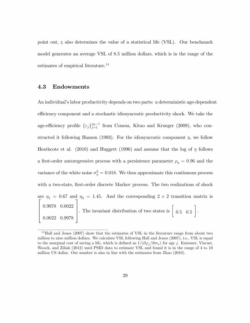
4.3 Endowments
An individual’s labor productivity depends on two parts: a deterministic age-dependent
effi ciency component and a stochastic idiosyncratic productivity shock. We take the
age-effi ciency profile {εj}jR−1j=1 from Conesa, Kitao and Krueger (2009), who con-
structed it following Hansen (1993). For the idiosyncratic component η, we follow
Heathcote et al. (2010) and Huggett (1996) and assume that the log of η follows
a first-order autoregressive process with a persistence parameter ρη = 0.96 and the
variance of the white noise σ2η = 0.018. We then approximate this continuous process
with a two-state, first-order discrete Markov process. The two realizations of shock
are η1 = 0.67 and η2 = 1.45. And the corresponding 2 × 2 transition matrix is 0.9978 0.0022
0.0022 0.9978
. The invariant distribution of two states is [ 0.5 0.5
].
14Hall and Jones (2007) show that the estimates of VSL in the literature range from about twomillion to nine million dollars. We calculate VSL following Hall and Jones (2007), i.e., VSL is equalto the marginal cost of saving a life, which is defined as 1/(∂ϕj/∂mj) for age j. Kniesner, Viscusi,Woock, and Ziliak (2012) used PSID data to estimate VSL and found it is in the range of 4 to 10million US dollar. Our number is also in line with the estimates from Zhao (2010).
29

4.4 Health Investment
We assume that the depreciation rate of health in equation (5) is age-dependent and
it takes the form
δhj =exp(d0 + d1j + d2j
2)
1 + exp(d0 + d1j + d2j2). (12)
This functional form guarantees that the depreciation rate is bounded between zero
and one and (given suitable values for d1 and d2) increases with age.
The production function for health at age j in equation (5) is specified as
g(mj) = Bmξj
where B measures the productivity of medical care, and ξ represents the return to
scale for health investment. Accordingly, we have five model-specific parameters
governing the health accumulation process: d0, d1, d2, B, ξ. We choose values of d0,
d1, and d2 to match three moment conditions regarding health status: average health
status from age 20 to 74, the ratio of health status for ages 20-29 to ages 30-39,
and the ratio of health status for ages 30-39 to ages 40-49.15 This results in d0 =
−4.3, d1 = 0.31, and d2 = 0.004. We calibrate B = 0.98 and ξ = 0.8 to match
15We choose to match the ratios of health status in earlier ages here is to leave the match of healthstatus in later life-cycle as out-of-sample prediction. The calibration here thus avoids data-fittingproblem.
30

two moment conditions regarding medical expenditure. B determines the scale of
medical expenditures. We thus calibrate it to match the medical expenditure-GDP
ratio, which was 15.1% in 2002.16 ξ determines the curvature of health production
technology. We calibrate it to match the average medical expenditure-labor income
ratio from age 20 to 64, which is 5.8%.17
4.5 Health Insurance
The MEPS data show that American retirees have about 80% of their medical ex-
penditures paid by health insurance. Medicare pays the majority of this (See De
Nardi et al. 2015 and Attanasio et al. 2010). For the working age population,
employer-based health insurance (EHI) pays the majority of medical expenditures.
The coverage rate of EHI is roughly 70-80%. Therefore, we set both coverage rates
for private insurance and Medicare at 80%.
4.6 Sick Time
Following Grossman (1972), we assume that sick time takes the form
s(hj) = Qh−γj (13)
16Data are from the National Health Accounts (NHA).17This ratio is calculated based on the data from panels a and d in Figure 1.
31

where Q is the scale factor and γ measures the sensitivity of sick time to health.
We calibrate these two parameters to match two moment conditions in the data.
Based on data from the National Health Interview Survey, Lovell (2004) reports
that employed adults in the US on average miss 4.6 days of work per year due to
illness or other health-related factors. This translates into 2.1% of total available
working days.18 We use this ratio as an approximation to the share of sick time
in total discretionary time over working ages. We choose Q = 0.005 to match this
ratio. Lovell (2004) also shows that the absence rate increases with age. For workers
between ages 45 to 64 years, it is 5.7 days per year which is 1.5 days higher than the
rate for younger workers between ages 18 to 44 years. We choose γ = 1.4 to match
the ratio of sick time for ages 45-64 to ages 20-44, which is 1.36.
4.7 Social Security
The Social Security replacement ratio κ is set to 40%. This replacement ratio is
commonly used in the literature (see for example, Kotlikoff, Smetters, and Walliser
1999 and Cagetti and De Nardi 2009).
18According to OECD data, American workers, on average, worked 1800 hours per year in 2004;that is equivalent to about 225 working days. Sick leave roughly accounts for 2.1% of these workingdays. This number is very close to the one reported in Gilleskie (1998).
32

4.8 Factor Prices
The wage rate w is set to be the average wage rate over working ages as estimated
from the PSID data as $12.03.19 The annual interest rate is set to be 4%.20 Therefore,
we obtain that r = (1 + 4%)5 − 1 = 21.7%.
Insert Table 1 here.
Insert Table 2 here.
5 Benchmark Results
Using the parameter values from Table 1, we compute the model using standard
numerical methods.21 Since we calibrate the model only to target selected aggregate
life-cycle ratios, the model-generated life-cycle profiles, which are shown in Figure 2,
can be compared with the data to inform us about the performance of the benchmark
19We first divide annual labor income for ages 20 to 64 from panel a in Figure 1 by the annualworking hours from panel b in Figure 1 to obtain wage rates wεjη across ages. We then divide
the average wage rate over working ages (w∑η
∑jR−1j=1 εjη
jR−1 ) by the product of average age-effi ciency∑jR−1j=1 εj
jR−1 and average (age-independent) idiosyncratic productivity shock (0.67 + 1.45)/2 to obtainaverage wage rate w, which is $12.03.204% is a quite common target for the return to capital in life-cycle models. See for example
Fernandez-Villaverde and Krueger (2011).21The computational method is similar to the one used in Imrohoroglu et al. (1995).
33

model.
Insert Figure 2 here.
Panel a in Figure 2 shows the life-cycle profile of health expenditures. Since one
model period represents five years in real life, a data point is an average for each five
year bin starting at age 20. Therefore, in the figure, age 22 represents age j = 1 in
the model and the average for ages 20-24 in the data, age 27 represents age j = 2
in the model and the average for ages 25-29 in the data, and so on. As we can
see, the model replicates the dramatic increase in medical expenditures in the data.
From ages 25-29 to ages 70-74, medical expenditure increases from $361 to $15068
in the data, while the model predicts that medical expenditures increase from $330
to $13194.
Health investment (in conjunction with depreciation) determines the evolution of
the health stock. Panel b in Figure 2 displays the life-cycle profile of health status.
The model produces decreasing health status over the life-cycle, which is consistent
with the data. For example, in the data, average health status (the fraction of
individuals who report being healthy) decreases from 0.9445 for ages 20-24 to 0.7625
for ages 60-64. The model predicts a change from 0.9445 to 0.7952.22
22In the computation, health stock h is discretized in the range of [0, 1]. The initial health stock
34

Since the survival probability is endogenous in the model, panel c in Figure 2
compares the model-generated survival probability with the data taken from US Life
Tables in 2002. The model almost perfectly matches declining survival probabilities
over the life-cycle in the data.
The model also does well in replicating other economic decisions over the life-
cycle. Panel d in Figure 2 shows the life-cycle profile of working hours. As can be
seen, the model replicates the hump shape of working hours. In the data, individuals
devote about 34% of their non-sleeping time to working at ages 20-24. The fraction
of working time increases to its peak at ages 35-39, and it is quite stable until ages
45-49. It then decreases sharply from about 38% at ages 45-49 to 22% at ages 60-64.
In the model, the fraction of working hours reaches its peak (about 38.2%) at ages
35-39 as in the data. It then decreases by 28%, to about 27% at ages 60-64. Since
we have a good fit for working hours, we also replicate the labor income profile in
the data quite well as can be seen in panel e in Figure 2.
Panel f in Figure 2 shows the life-cycle profile of consumption (excluding medical
expenditure) in the model. Similar to the data displayed in Figure 1 in Fernandez-
Villaverde and Krueger (2007), it exhibits a hump shape. Fernandez-Villaverde and
Krueger (2007) measure the size of the hump as the ratio of peak consumption to
h1 is set to be 0.9445 which is the fraction of the population aged 20-24 who report being healthyin the data.
35

consumption at age 22 and they obtain a ratio of 1.60. In our model this ratio
is 1.7 which is close to the data. A noticeable difference between the model and
the data is the sharp drop in consumption right after retirement in the model. The
reason is the non-seperability between consumption and leisure in the utility function.
Consumption and leisure are substitutes in our benchmark preferences. Retirement
creates a sudden increase in leisure and, hence, substitutes for consumption after
retirement.23
To summarize, our life-cycle model with endogenous health accumulation is able
to replicate life-cycle profiles from the CEX, MEPS, and PSID. First, it replicates
the hump shape of consumption. Second, it replicates the hump shape of working
hours and labor income. Third and most important, it replicates rising medical
expenditures and decreasing health status and survival probabilities over the life-
cycle.
23A sudden drop in consumption after retirement is common in the literature that uses non-separable utility functions, e.g., Conesa et al. (2009). Bullard and Feigenbaum (2007) show thatconsumption-leisure substitutability in household preferences may help explain the hump shape ofconsumption over the life-cycle. As evidence, when we use an alternative preference with a separableutility function between consumption and leisure in an unreported experiment with the deterministicversion of the model, we obtain a much smoother consumption profile around retirement age.
36

6 Decomposition of Health Investment Motives
Based on the success of the benchmark model, we run a series of experiments to
quantify the relative importance of the three motives for health investment as shown
in equation (7). To obtain an idea of the magnitude of each motive in the Euler
equation, we directly plot the three terms in equation (7) in Figure 3 generated
from the benchmark model. The figure shows that the I-Motive dominates the other
two motives prior to the late 50s but is taken over by the C-Motive after. Unlike
the other two motives, the I-Motive decreases over the working ages. This is a
consequence of the interplay between increasing leisure over working ages and the
declining marginal gain of reducing sick time from health improvement (i.e., given
our calibration, s′′(h) < 0) over working age.
In contrast to the I-Motive, the importance of the C-Motive increases monoton-
ically with age. This is because health directly enters into the utility function as a
consumption commodity and because health is decreasing over time due to natural
depreciation. The scarcity of the health stock late in life pushes up the marginal
utility of health and encourages rising health investment. After the early 60s, rising
medical expenditures are driven more by the consumption than the investment mo-
tive. Finally, as shown in the figure, although its importance is increasing as people
age, the S-Motive is quantitatively much less important than the other two motives.
37

Insert Figure 3 here.
6.1 Decomposition without Recalibration
Figure 3 gives us some sense of the relative importance of each motive within the
benchmark model. In order to see the impact of each motive on endogenously deter-
mined medical expenditures, we run a series of counterfactual experiments. In the
first three experiments, we isolate each motive within the benchmark model.
The three experiments are as follows. “No C-Motive”is a model in which we shut
down the consumption motive by setting λ = 1 while keeping all other parameters at
their benchmark values. Since health status does not enter into the utility function,
the first term inside the bracket of equation (7) disappears. “No I-Motive”is a model
without the investment motive which obtains by settingQ = 0 while keeping all other
parameters at their benchmark values. Since there is no sick time in the model, the
second term in equation (7) vanishes. “No S-Motive”is a model without the survival
motive that obtains by setting $3 = 0 while keeping all other parameters at their
benchmark values. Because health does not affect survival, the third term in equation
(7) vanishes. Notice that when we shut down one motive from the benchmark model,
we do not recalibrate the model. This helps us to understand the mechanism behind
38

each motive. In addition, since we do not recalibrate the model, the three alternative
scenarios mentioned below maintain the same parameter values except for those that
have been shut down. This exercise thus helps us to identify the relative importance
of each motive in determining medical expenditures at different periods in the life-
cycle. We plot the model-generated life-cycle profile of medical expenditure under
the three scenarios in Figure 4.
Insert Figure 4 here.
As shown in Figure 4, when compared to the benchmark model, medical expen-
ditures in the No C-Motive model are significantly lower than that the benchmark
model throughout the life-course, especially after the late 50s. Hence, the consump-
tion motive accounts for a significant part of medical expenditures. On the other
hand, the No I-Motive model predicts even lower medical expenditures than in the
No C-Motive and No S-Motive cases prior to the early 40s, implying that the in-
vestment motive is quantitatively more important than the consumption motive in
driving up medical expenditures before age 50. However, after the early 50s, the
difference between the No I-Motive case and the benchmark model is much smaller
than the difference between the No C-Motive case and the benchmark model. It indi-
cates that the investment motive is dominated by the consumption motive in driving
39

up medical expenditures at later ages. Finally, the No S-Motive model implies that
medical expenditures are lower than in the benchmark model with the difference get-
ting bigger as people age, especially towards the end of the life-cycle. The survival
motive is quantitatively much less important than the other two motives, especially
when compared to the consumption motive. Overall, the message about the relative
importance of each motive in Figure 4 is consistent with the one conveyed in Figure
3.
Differences in medical expenditures determine differences in health status, which
in turn, affects survival. Panel a in Figure 5 shows that the No C-Motive model
generates a significantly lower health stock than in the benchmark model (and the
data), particularly after retirement. Consistent with both Figures 3 and 4, the No
I-Motive model predicts a lower health stock than that in the No C-Motive and No
S-Motive case prior to the late 40s. However, after retirement, the impact of the
I-Motive on health status significantly decreases. In contrast, the C-Motive becomes
more important which is consistent with Figures 3 and 4.
Finally, panel b in Figure 5 reports the effect of the three motives on survival.
Since the No S-Motive case directly shuts down the role that health plays in survival,
we see that the No S-Motive model predicts lower survival throughout the entire
life-cycle than that in the benchmark case. The other two motives affect survival
40

indirectly via their effect on health status. The results, however, show that their
impact on survival is not quantitatively significant.
Insert Figure 5 here.
To some extent, the low importance of the S-Motive is surprising since one would
think an important feature of the value of health is to extend life span (as modeled
in Suen 2006 and Zhao 2010). However, notice that our model also includes the
explicit feature of consumption value for health (i.e., health directly enters into utility
function). In other words, health in our model not only extends one’s life span, but
also improves the quality of life. In that sense, the combination of the C-Motive and
the S-Motive in our model is isomorphic to the role that health plays in the literature
such as Suen (2006) and Zhao (2010). Our decomposition exercise thus provides a
deeper understanding of the reason why people value health over the life-cycle. By
differentiating the C-Motive from the S-Motive, we show that an individual invests
in health mainly because health improves the quality of life, not because health
simply extends the length of life. Additionally, notice that the functional form of
the survival probability in equation (10) makes the conditional survival probability
depend on, not only, health status but also age. In other words, a large of fraction
of the declining survival probability over the life-cycle comes from biological aging.
41

This functional form further mitigates the impact of the health stock on the survival
probability and, hence, contributes to the marginal importance of the S-Motive.
6.2 Decomposition with Recalibration
The dominance of the C-Motive that we have seen, however, might be a result of a
mechanical implication of the model. The reason is that the C-Motive is the only
motive with a first order effect on the agents’decision problem via preferences. As
a result, it should play the most important role in the calibration and, so removing
it will generate the biggest loss in terms of model fit. To mitigate this concern
and hence to evaluate the overall importance of each motive, a better exercise is
to recalibrate the three scenarios mentioned above to give each model a chance to
match the data moments again. With the model being recalibrated and returned to
the same starting point and by looking at the fit of these three recalibrated models
separately, one will be able to determine the overall importance of each motive. In
other words, if the model can be easily recalibrated to match the data again while
shutting down a specific motive, this shows that this motive is not quantitatively
important. Otherwise, it is.
To implement the exercise, we recalibrate nine out of sixteen calibrated para-
meters in Table 1 for each alternative model. The spirit of recalibration requires
42

us to recalibrate all five parameters on preference (β, ψ, ρ, λ, and c¯) since they
are the most relevant parameters related to the first order effect and the other four
decision-related technological parameters: B, ξ for health production, and Q, γ for
the sick time function. The remaining seven parameters, $0, $1, $2, and $3, govern
the survival probability and d0, d1 and d2 determine the age-dependent depreciation
rate of health. They are relatively much more “exogenous”to the nine “behavioral”
parameters we recalibrate in the sense that they are determined largely by biological
processes rather than economic behavior. Therefore, we choose not to recalibrate
them so that each alternative model faces the same “biological”parameter values as
in the benchmark model.24
We plot the model-generated life-cycle profile of medical expenditures under the
benchmark and under three alternative recalibrated models in Figure 6. The figure
shows a somewhat different message compared to Figure 4. Both the “No I-Motive”
and “No S-Motive”models can almost replicate the benchmark model (and hence the
data) except in later ages. In contrast, the “No C-Motive”model, although matched
with the moment conditions in Table 2 to our best effort, cannot replicate the life-
cycle profile of medical expenditures in the benchmark model and data. Even after
24In an unreported exercise, together with the nine recalibrated “behavioral”parameters, we alsorecalibrate ω3 which governs the sensitivity of health stock to survival probability for each scenario(except for “No S-Motive”case). We find the results are very similar to the one reported in Figure6.
43

mitigating the possible mechanical advantage of the C-motive, it still dominates all
other possible drivers of the rise in medical expenditures over the life-cycle. Figure
6, thus, confirms the overall importance of the consumption motive in driving up
health investment over the life-cycle.
Insert Figure 6 here.
7 Counterfactual Policy Experiments
Our benchmark model offers a quantitative analysis of health investment over the
life-cycle in a framework featuring various roles of health. Our focus on the life-
cycle enables us to make statements about how policies will affect health investment
behavior over the life-cycle and distribute medical resources across generations and
individuals, which is something that previous work on health investment does not do.
With various roles of health in the model, we are also able to provide a comprehensive
analysis of the possible impact of different policies on health expenditures and health
status.
The model setting allows us to consider three sets of policy changes. First, our
benchmark model summarizes the subsidized nature of the US health insurance sys-
tem. The government can impact behavior by changing the coverage rates of pub-
44
lic health insurance, φp and φm. Second, from equations (7) and (8), one can see
that Social Security policy as embedded in the parameters, {τ ss, κ, jR}, will affect
the investment motive for working age people. We have learned from the previous
section that this motive is important in determining medical expenditures prior to
retirement. Third, the government can also indirectly affect health investment by
encouraging technological change in the medical sector via increases in B.
In this section, we run a series of counterfactual experiments that quantitatively
investigate the effects of these policies on health investment behavior. In addition, we
are also able to show the impacts of the policies on the aggregate medical expenditure-
national income ratio and social welfare. However, as we emphasized in the intro-
duction, due to the partial equilibrium structure of the model, we have to provide a
caveat when interpreting these results on aggregate ratios and welfare.
7.1 Subsidized Health Insurance
The benchmark framework in Section 2 explicitly models the heavily subsidized na-
ture of medical spending in the US. A natural question one could ask is how changes
in health insurance coverage rates (φm and φp) affect medical expenditures. In this
section we run an experiment in which we decrease both coverage rates from their
benchmark value of 80% to 40% and 0%, respectively, while keeping the other para-
45

meters constant at their benchmark values.
Panel a in Figure 7 shows that by reducing the health insurance coverage rates,
φm and φp, simultaneously, medical expenditures decrease quite significantly over
the entire life-course. This decrease is especially pronounced in late ages. This
subsidy to medical expenditures makes medical care cheaper relative to non-medical
consumption and hence encourages more usage of health care (the relative price of
medical goods to non-medical consumption is 1 − φj). Thus, reducing it makes
individuals more cautious when using medical services. This can be seen clearly
when one looks at the Euler equation (7). Notice that reducing the coverage rate φj
decreases the right-hand side of equation (7), which represents marginal benefit of
health investment. Lower medical expenditures over the life-cycle also lead to worse
health status, as shown in panel b of Figure 7.
Insert Figure 7 here.
On the aggregate level, as shown in Table 3, when we reduce insurance coverage
rates, individuals are more cautious when using medical services, which leads to a
substantial reduction in the medical expenditure-national income ratio from 16.0%
to 11.2% at φp = φm = 40% and to 9.4% at a zero coverage rate. Reducing insurance
coverage rates also makes investment in physical capital relatively more attractive
46

compared to investment in health capital, which encourages asset holdings and hence
increases the capital-wealth ratio.
Finally, we calculate the welfare implications of different insurance coverage rates
compared to the benchmark model. First, following Imrohoroglu, Imrohoroglu and
Joines (1995), we use the expected life time utility of a newborn
U(c, l, h) = EJ∑j=1
βj−1
[j∏
k=1
ϕk(hk)
]u(cj, lj, hj)
to measure social welfare, with the period utility function defined as in equation
(11). For the benchmark model, we have the allocation (cb, lb, hb) and the associated
utility U(cb, lb, hb). For each policy change, we have the new allocation (c∗, l∗, h∗)
and the associated utility U(c∗, l∗, h∗). Then following the literature (e.g., Conesa
et al. 2009 and Fehr et al. 2013), the welfare consequence of switching from the
steady-state benchmark allocation (cb, lb, hb) to an alternative allocation (c∗, l∗, h∗),
or the consumption equivalent variation (CEV) of the policy change is
CEV =
[U(c∗, l∗, h∗)
U(cb, lb, hb)
]1/(1−σ)− 1
We report the CEV calculation in the eighth column of Table 3. It shows that
reducing insurance coverage rates and hence the subsidy of medical consumption
47

brings a significant welfare gain to the economy. Reducing insurance coverage rates
encourages individuals to invest more in physical capital, which leads to higher output
(shown in the seventh column in Table 3). This is the main source of the welfare
gain.
Insert Table 3 here.
7.2 Changing the Replacement Ratio
Changing the replacement ratio is often cited as a means of shoring-up Social Security
in the U.S. and elsewhere. Clearly, such a policy would affect Social Security taxes
and benefits, but whether it would affect medical expenditures remains an open
question. In this section, we run a counterfactual experiment where we change
the replacement ratio, κ, from its benchmark level of 40% to 0%, 20% and 60%,
respectively, while keeping the other parameters at their benchmark values.
Insert Figure 8 here.
Figure 8 shows the life-cycle profiles of asset holdings and total income (labor plus
capital income) generated by different values of κ. In our model, the main motive for
savings is to support consumption (both non-medical and medical consumption) in
48

old age. Therefore, it is not surprising to see that a lower replacement ratio, which
implies lower Social Security benefits after retirement (see the third column in Table
4), will induce agents to save more over the entire life-cycle. This is consistent with
findings in Imrohoroglu et al. (1995). The effect is also shown in Table 4; as the
replacement ratio κ decreases, the capital-wealth ratio K/Y increases. Partly due
to a lower tax rate τ ss caused by lower κ (shown in the second column in Table 4)
and partly due to higher asset holdings, panel b in Figure 8 shows that total income
during working ages is also higher when the replacement ratio is smaller.
Insert Figure 9 here.
Figure 9 shows the life-cycle profiles of medical expenditures and health status
for different κ. Panel a shows that a lower replacement ratio generally leads to higher
medical expenditures during working ages. To understand the intuition of this quite
surprising result, we have to refer back to the Euler equation (7). For working age
agents, we know that the investment motive is
((1− τ ss − τmed)wεj+1
∂u
∂cj+1+κwεj+1jR − 1
J∑p=jR
(βp−j−1
[p∏
k=j+2
ϕk(hk)
]∂u
∂cp)
)s′(hj+1).
Note that both the Social Security tax rate τ ss and the replacement ratio κ enter the
49

expression. The government must balance its budget since the Social Security system
is self-financing. Therefore, a lower replacement ratio also leads to a lower Social
Security tax rate τ ss as shown in the second column of Table 4. A lower τ ss tends to
increase the magnitude of the investment motive by increasing current after-tax labor
income. In contrast, a lower κ in the same term tends to reduce the magnitude of
I-Motive. Its impact, however, is lower since it affects utility via its impact on future
labor income that is the base for Social Security benefits, which is discounted by both
the time preference and the conditional survival probability. Therefore, other things
equal, a lower κ leads to a higher investment motive for working age agents, and
hence results in higher medical expenditures. Another channel that affects health
investment is total income. With substantially higher asset holdings for lower values
of κ, total income is higher, which is also shown in the eighth column of Table 4.
For example, for κ = 0, total income is about 24% higher than the benchmark case
with κ = 40%. Since medical care is a normal good, higher income leads to higher
medical expenditures due to income effect.
However, notice that this pattern is overturned towards the end of the life-cycle.
Medical expenditures under a replacement ratio of 40% (benchmark case) are higher
than medical expenditures under a replacement ratio of either 0% or 20% after the
early 80s. Moreover, medical expenditure under a replacement ratio of 60% are
50

higher than the medical expenditure when generated by any other lower replace-
ment ratio after the late 70s. Our intuition here is that, because the Social Security
system redistributes resources from workers to retirees, retirees have a higher mar-
ginal propensity to consume medical goods.25 Therefore higher replacement ratios
drives up medical expenditures, especially at late ages since the redistribution effect
dominates. This is the main point made in Zhao (2010). This exercise confirms it
quantitatively.
Since a lower κ, in general, generates higher medical expenditures over the life-
cycle, it is not surprising to see in panel b of Figure 9 that a lower κ also leads to
better health. Hence, as shown in the seventh column of Table 4, which computes
average health status from age 20 to 90, when κ decreases from 40% to zero, average
health status for ages 20-90 increases from 0.815 to 0.835.
The sizable changes in medical expenditures over the life-cycle caused by dif-
ferent replacement ratios also translate to sizable changes in aggregate medical ex-
penditures. As shown in the fourth column of Table 4, when κ decreases from
40% to zero, the M/Y ratio decreases from 16.0% to 13.6%. This is somewhat
counter-intuitive since smaller κ increases medical expenditures over the major part
of life-cycle. However, this puzzle is resolved once we consider that lower κ increases
25As an evidence of the redistribution effect, as shown in panel b in Figure 8, total income ofretirees is higher when replacement ratio κ is higher.
51

capital accumulation but does not decrease labor supply (the sixth column shows the
average fraction of working hours in discretionary time over working age)26, so the
denominator of the ratio increases by a greater amount than the numerator (which
is shown in the eighth column for comparison of GDP to the benchmark level).
Finally, we report the CEV for each policy change in the ninth column of Table 4.
The results show that, in the current model, a reduction in the replacement ratio im-
proves welfare and that a zero replacement ratio, i.e. privatization of Social Security,
delivers the highest social welfare. These results are consistent with other findings
in literature such as Kotlikoff, Smetters, and Walliser (1999) and Imrohoroglu and
Kitao (2009b). Importantly, neither of these papers models health.
Insert Table 4 here.
7.3 Delaying Retirement
Many proposals to reform Social Security suggest that the retirement age will have
to be postponed by a few years. In this section, we run an experiment in which
we delay the retirement age jR by one more period from jR = 10 to jR = 11 while
26Lower tax rate τss will make individuals increase labor supply due to substitution effect. How-ever, lower tax will also have strong income effect which leads to reduction of labor supply. Theincome effect cancels out the substitution effect. Therefore labor supply in the sixth column ofTable 4 remains almost constant across different κ.
52
keeping the other parameters at their benchmark values. This corresponds to an
increase in the retirement age from 65 to 70.
Insert Figure 10 here.
Figure 10 shows the life-cycle profiles of assets, medical expenditures and health
status when the retirement age is delayed for one period in the model. Panel a shows
that due to the delay, an individual increases asset holdings over the life-cycle. The
main reason is that now the agent works for a longer period and, hence, her labor
income increases enabling her to save more. Panels b and c show that this policy
change would not significantly affect medical expenditures and health status.
On the aggregate level, as shown in Table 5, we can see that by delaying retire-
ment, the number of workers increases and the pool of retirees shrinks. Accordingly,
the Social Security tax rate τ ss significantly decreases. The Social Security benefit,
however, does not decrease much. The reformed Social Security system decreases
the medical expenditure-national income ratio from 16.0% to 15.0%. This decrease
is not due to changes in medical expenditures, but rather increases in total income
as shown in the eighth column of the table, which in turn is due to increases in both
capital accumulation and labor supply as shown in the fifth and sixth column of the
53

table.27 Finally, since higher income leads to higher consumption and better health,
delaying the retirement age increases social welfare, which is equivalent to a 1.95
percent increase in the allocation of consumption-leisure-health as compared to the
benchmark one.
Insert Table 5 here.
7.4 Encouraging Health Care Technological Change
Technological improvement in health care services has been cited as a major reason
for the rising medical expenditure-GDP ratio in the US (see Suen 2006). There are
a variety of policies that the government can pursue that could possibly accelerate
this technological change (e.g., more funding for the National Institute of Health,
tax favorable treatment on R&D in drugs, etc.). We now investigate what would
happen in the current model if the medical service sector TFP increases.
In our benchmark model, the TFP of medical care technology is calibrated to be
0.98. We analyze two hypothetical scenarios. First, B increases by 10% (to 1.078)
and then to 20% (to 1.176). We keep all other parameters at their benchmark values.
Panel a in Figure 11 shows that increasing B reduces medical expenditures over
27Sixth column shows the average labor supply (as a fraction of discretionary time) for ages 20-65.
54
the life-cycle, especially after the mid 50s. However, panel b in the same figure reports
that health status improves despite health investment decreasing, which indicates
that the effi ciency of health investment increases. This is consistent with the original
Grossman model.
Insert Figure 11 here.
Why does an increase inB reduce medical expenditures over the life-cycle? Notice
that B affects the marginal product of medical expenditure in the health production
technology, g′(mj). Therefore, on one hand an increase in B raises g′(mj) in the
Euler equation (7) and hence increases the marginal benefits of health investment
which, in turn, leads to higher medical expenditures over the life-cycle. On the
other hand, under our calibration, the elasticity of substitution between health and
the non-medical consumption-leisure combination is strong enough so that improving
health leads to an increase in non-medical consumption, which “crowds out”medical
consumption. Under our calibrated parameter values, the latter dominates the former
channel.28
28In an unreported experiment, when we set ψ = −900 and hence elasticity of substitution be-tween health and c-l combination is extremely small (=0.001), the change in health would notinduce significant change in non-medical consumption. Therefore the “crowding-out”effect is elim-inated. The impact of B on M/Y ratio is mainly determined by the first channel. As we expect,in that case, M/Y increases to 16.3% when B increases by 10%. On the other hand, if we setψ = 0 so that elasticity of substitution is much larger than its benchmark value, we strengthen the
55
Finally, by raising GDP (shown in the sixth column in Table 6), non-medical
consumption (the C/Y ratio increases by 0.44% and 1.08% respectively for two cases)
and health status (shown in the fifth column of Table 6), increasing B increases social
welfare by 0.56% and 1.05% respectively.
Insert Table 6 here.
To summarize, based on the current model, policies that try to reduce subsidies
to health insurance, shore-up Social Security either by lowering the replacement ratio
or by delaying the retirement age, and improve technological productivity decrease
medical expenditures over the life-cycle and reduce the medical expenditure-GDP ra-
tio. All of these policies deliver welfare gains when compared to the current system.
Among those policies, reducing insurance subsidies and the social security replace-
ment ratio have the largest impacts on medical expenditures and social welfare.
8 Conclusions
We studied the life-cycle behavior of health investment and its effects on other aspects
of consumer behavior. Specifically, we asked ourselves what drives the increase in
“crowding-out”effect. Therefore M/Y ratio decreases even more significantly to 11.45% when Bincreases by 10%.
56

medical expenditures over the life-cycle. Three motives for health investment were
considered. First, health delivers a flow of utility each period (the consumption
motive). Second, better health enables people to allocate more time to productive
or pleasurable activities (the investment motive). Third, better health increases
longevity (the survival motive). We calibrated an overlapping generations model
with endogenous health investment, worker heterogeneity, and a realistically modeled
health insurance system by matching various ratios from the model and US data. We
found that the calibrated model fits key life-cycle profiles of consumption, working
hours, health status, medical expenditures, and survival very well.
Based on the success of the benchmark model, we ran a decomposition exercise
to quantify the relative importance of each motive. We found that, overall, the con-
sumption motive plays a much more important role in shaping health expenditures
over the life-cycle. Focusing on different episodes of the life-cycle, we found that
the investment motive is more important than the consumption and survival mo-
tives until the 40s. After that, the consumption motive is the dominant force behind
health investment. In other words, younger people invest in their health because
better health allows them to enjoy more leisure or to work more, while older people
invest in their health because better health improves their quality of life. Finally,
the survival motive is quantitatively less important than the other two motives.
57

We conducted a series of counterfactual experiments to investigate how govern-
ment policies that reduce health insurance coverage rates, shore-up Social Security,
and accelerate technological progress in medicine affect the life-cycle behavior of
health investment, and the aggregate medical expenditure-GDP ratio. We found
that all of these policies decrease medical expenditures over the life-cycle and reduce
the medical expenditure-GDP ratio. They also yield welfare gains as compared to
the benchmark system. Among those policies, reducing insurance coverage rates and
the social security replacement ratio have a much more significant impact on medical
expenditures and social welfare than the other policies.
Our model can be extended along several dimensions. First, we assumed exoge-
nous factor prices for simplicity. Therefore, the model does not capture feedback
effects from factor prices. Future work could extend the model by allowing for en-
dogenous factor prices in order to investigate general equilibrium effects. Second, we
assumed a mandatory retirement at age 65 in the model. In the future, researchers
may want to endogenize retirement to shed light on the effects of health on retirement
behavior in a setting with endogenous health. Finally, there is no health uncertainty
in the model. Adding uncertainty would allow us to analyze the effects of health
insurance against idiosyncratic medical expenditure shocks on an individual’s health
investment. It will also generate more heterogeneity in medical expenditures across
58

individuals of the same age. We leave those topics for future research.
References
[1] Attanasio, Orazio, Sagiri Kitao, and Giovanni L. Violante (2010) Financing
medicare: A general equilibrium analysis. In Demography and the Economy
(pp. 333-366). University of Chicago Press.
[2] Baker, Michael, Mark Stabile, and Catherine Deri (2004) What do self-reported,
objective, measures of health measure?. Journal of Human Resources 39, 1067-
1093.
[3] Batinti, Alberto (2015) On medical progress and health care demand: a ces
perspective using the grossman model of health status. Health Economics 24,
1632-1637.
[4] Bloom, David E., David Canning, and Bryan Graham (2003) Longevity and
life-cycle savings. The Scandinavian Journal of Economics 105, 319-338.
[5] Bloom, David E., David Canning, and J. Sevilla (2005) Health and economic
growth: reconciling the micro and macro evidence. Center on Democracy, De-
velopment and the Rule of Law Working Papers, 42.
59
[6] Bound, John (1991) Self-reported versus objective measures of health in retire-
ment models. Journal of Human Resources 26, 106-138.
[7] Bullard, James and James Feigenbaum (2007) A leisurely reading of the life-
cycle consumption data. Journal of Monetary Economics 54, 2305-2320.
[8] Cagetti, Marco and Mariacristina De Nardi (2009) Estate taxation, entrepre-
neurship, and wealth. The American Economic Review 99, 85-111.
[9] Carroll, Christopher D (1997) Buffer-stock saving and the life cycle/permanent
income hypothesis. The Quarterly Journal of Economics 112, 1-55.
[10] Conesa, Juan Carlos, Sagiri Kitao, and Dirk Krueger (2009) Taxing capital?
Not a bad idea after all!. The American Economic Review 99, 25-48.
[11] Cagetti, Marco and Mariacristina De Nard (2006) Wealth inequality: Data and
models. Macroeconomic Dynamics 12, 285-313.
[12] De Nardi, Mariacristina, Eric French, and John Bailey Jones (2009) Life ex-
pectancy and old age savings. The American Economic Review 99, 110-15.
[13] De Nardi, Mariacristina, Eric French, and John Bailey Jones (2009) Why do the
elderly save? the role of medical expenses. Journal of Political Economy 118,
39-75.
60

[14] De Nardi, Mariacristina, Eric French, John Bailey Jones, and McCauley Jeremy
(2015) Medical spending on the U.S. elderly. National Bureau of Economic Re-
search, No. w21270.
[15] Deaton, Angus (1992) Understanding consumption. Oxford University Press.
[16] Fehr, Hans, Manuel Kallweit, and Fabian Kindermann (2013) Should pensions
be progressive. European Economic Review 63, 94-116.
[17] Feng, Zhigang (2012). Macroeconomic consequences of alternative reforms to
the health insurance system in the US. Available at SSRN 2037058.
[18] Fernandez-Villaverde, Jesus and Dirk Krueger (2007) Consumption over the life
cycle: Facts from consumer expenditure survey data. The Review of Economics
and Statistics 89, 552-565.
[19] Fernandez-Villaverde, Jesus and Dirk Krueger (2011) Consumption and saving
over the life cycle: How important are consumer durables?. Macroeconomic
Dynamics 15, 725-770.
[20] Finkelstein, Amy, Erzo FP Luttmer, and Matthew J. Notowidigdo (2013) What
good is wealth without health? The effect of health on the marginal utility of
consumption. Journal of the European Economic Association 11, 221-258.
61

[21] Fonseca Raquel, Michaud Pierrecarl, Galama Titus, and Kapteyn Arie (2009).
On the rise of health spending and longevity. IZA Discussion paper #4622.
[22] French, Eric (2005) The effects of health,wealth, and wages on labour supply
and retirement behaviour. Review of Economic Studies 72, 395—427.
[23] Gilleskie, Donna B (1998) A dynamic stochastic model of medical care use and
work absence. Econometrica 66, 1-46.
[24] Gourinchas, Pierreolivier and Jonathan A. Parker (2000) Consumption over the
life-cycle. Econometrica 70 , 47-89.
[25] Grossman, Michael (2015) On the concept of health capital and the demand for
health. Journal of Political Economy 80, 223-55.
[26] Hall, Robert E. and Charles I. Jones (2007) The value of life and the rise in
health spending. Quarterly Journal of Economics 122, 39-72.
[27] Hanse, Gary (1993) The cyclical and secular behaviour of the labour input:
Comparing effi ciency units and hours worked. Journal of Applied Econometrics
8, 71-80.
62

[28] He, Hui and Huang, Kevin XD (2013) Why do Americans spend so much more
on health care than Europeans?—A general equilibrium macroeconomic analysis,
Vandebilt University, Working Paper.
[29] Heathcote, Jonathan, Kjetil Storesletten, and Giovanni L. Violante (2008) The
macroeconomic implications of rising wage inequality in the United States. Jour-
nal of Political Economy 118, 681-722.
[30] Huang, He, Imrohoroglu, Selahattin, and Thomas J. Sargent (1997) Two com-
putations to fund social security. Macroeconomic Dynamics 1, 7-44.
[31] Huang, Kevin XD and Gregory W. Huffman (2014) A defense of the current US
tax treatment of employer-provided medical insurance. Macroeconomic Dynam-
ics 18, 1547-1580.
[32] Hubbard, Glenn, Jonathan S. Skinner, and Stephen P. Zeldes (1994) The impor-
tance of precautionary motives in explaining individual and aggregate saving.
Journal of Monetary Economics 40, 59-125.
[33] Huggett, Mark (1996) Wealth distribution in life-cycle economies. Journal of
Monetary Economics 38, 469-494.
63

[34] Imrohoroglu, Selahattin and Sagiri Kitao (2009a) Social security, benefit claim-
ing and labor force participation: A quantitative general equilibrium approach.
unpublished mimeo.
[35] Imrohoroglu, Selahattin and Sagiri Kitao (2009b) Labor supply elasticity and
social security reform. Journal of Public Economics 93, 867-878.
[36] Imrohoroglu, Ayse, Selahattin Imrohoroglu, and Douglas H. Joines (1995) A life
cycle analysis of social security. Economic Theory 6, 83-114.
[37] Jeske, Karsten and Sagiri Kitao (2007) U.S. tax policy and health insurance
demand: Can a regressive policy improve welfare?. Journal of Monetary Eco-
nomics 56, 210-221.
[38] Jung, Juergen and Chung Tran (2009) The macroeconomics of health savings
accounts. Towson University, Department of Economics, No. 2010-12.
[39] Jung, Juergen and Chung Tran (2010) Medical consumption over the life-cycle:
Facts from a U.S. medical expenditure panel survey. Available at SSRN 1560484.
[40] Kashihara David and Carper Kelly (2008) National health care expenses in the
US civilian non-institutionalized population, 2009. Medical Expenditure Panel
Survey Statistical Brief #229.
64
[41] Kinugasa, Tomoko and Andrew Mason (2007) Why countries become wealthy:
the effects of adult longevity on saving. World Development 35, 1-23.
[42] Kniesner, Thomas, Viscusi, W. Kip, Woock, Christopher, and Ziliak, James
P. (2012). The value of a statistical life: Evidence from panel data. Review of
Economics and Statistics 94, 74-87.
[43] Kopecky, Karen A. and Koreshkova Tatyana (2009) The impact of medical and
nursing home expenses and social insurance policies on saving and inequality.
unpublished mimeo.
[44] Kotlikoff, Laurence J., Kent Smetters, and Jan Walliser (1999) Privatizing so-
cial security in the United States– comparing the options. Review of Economic
Dynamics 2, 532-574.
[45] Lillard, Lee A. and Robert J. Willis (1978) Dynamic aspects of earning mobility.
Econometrica 46, 985-1012.
[46] Lovell, Vicky (2004) No time to be sick: Why everyone suffers when workers
don’t have paid sick leave. IWPR Publication #B242p, Institute for Women’s
Policy Research, Washington DC.
[47] Meara, Ellen, Chapin White, and David M. Cutler (2004) Trends In medical
spending by age, 1963—2000. Health Affairs 23, 176-183.
65

[48] Meghir, Costas and Luigi Pistaferri (2002) Income variance dynamics and het-
erogeneity. Econometrica 72, 1-32.
[49] Ozkan, Serdar (2010) Income differences and health care expenditures over the
life-cycle. unpublished mimeo.
[50] Palumbo, Michael G. (1999) Uncertain medical expenses and precautionary sav-
ing near the end of the life cycle. The Review of Economic Studies 66, 395-421.
[51] Podor, Melinda and Timothy Halliday (2012) Health status and the allocation
of time. Health Economics 21, 514-527.
[52] Rust, John and Christopher Phelan (1997) How social security and Medicare
affect retirement behavior in a world of incomplete markets. Econometrica 65,
781-831.
[53] Smith, James P. (2003) Health and SES over the life-course. unpublished mimeo.
[54] Suen, Richard (2006) Technological advance and the growth in health care
spending. unpublished mimeo.
[55] Viscusi, W. Kip and William N. Evans (1990) Utility functions that depend on
health status: estimates and economic implications. The American Economic
Review 80, 353-374.
66

[56] Yogo, Motohiro (2016) Portfolio choice in retirement: Health risk and the de-
mand for annuities, Housing and Risky Assets. unpublished mimeo.
[57] Zhao, Kai (2010) Social security and the rise in health spending: A macroeco-
nomic analysis. unpublished mimeo.
67

9 Tables and Figures
68

Parameter Description Value SourceDemographics
J maximum life span 16 age 95-99jR mandatory retirement age 10 age 65-69$0 survival prob. −5.81 calibrated$1 survival prob. 0.285 calibrated$2 survival prob. 0.0082 calibrated$3 survival prob. −0.17 calibrated
Preferencesβ subjective discount rate (0.975)5 calibratedσ Intertem. ela. sub. coeffi cient 2 common valueψ elasticity b/w cons. and health −9.7 calibratedρ share of c in c-leisure combination 0.342 calibratedλ share of cons-leisure com. in utility 0.97 calibratedc¯
constant term in utility 2.3 calibratedHealth Accumulation
d0 dep. rate of health −4.3 calibratedd1 dep. rate of health 0.31 calibratedd2 dep. rate of health 0.004 calibratedB productivity of health technology 0.98 calibratedξ return to scale for health investment 0.8 calibrated
Sick TimeQ scale factor of sick time 0.005 calibratedγ elasticity of sick time to health 1.4 calibrated
Labor Productivity{εj}jR−1j=1 age-effi ciency profile Conesa et al. (2009)ρη persistence of productivity shock 0.96 Heathcote et al. (2010)ση variance of productivity shock 0.018 Heathcote et al. (2010)
Health Insuranceφp coverage rate, private insurance 0.8 MEPS dataφm coverage rate, Medicare 0.8 MEPS data
Social Securityκ Social Security replacement ratio 40% Kotlikoff et al. (1999)
Factor Pricesw wage rate $12.03 PSIDr interest rate 0.2167 Fernandez-Villaverde et al. (2011)
Table 1: Parameters of the model
69

Target (Data source) Data ModelCapital-output ratio (NIPA) 2.6 2.5Non-med. consumption-labor income ratio (CEX and PSID) 78.5% 71.2%Med. expenditure (ages 55-74)/(ages 20-54) (MEPS) 7.96 7.93Fraction of average working hours (PSID) 0.349 0.347Med. expenditure-output ratio (NHA) 15.1% 16.0%Med. expenditure-labor income ratio (MEPS and PSID) 5.8% 4.9%Fraction of average sick time (ages 20-64) (Lovell 2004) 2% 1%Sick time (ages 45-64)/Sick time (ages 20-44) (Lovell 2004) 1.36 1.19Average health status (ages 20-74) (PSID) 0.845 0.863health (ages 20-29)/health (ages 30-39) (PSID) 1.02 1.02health (ages 30-39)/health (ages 40-49) (PSID) 1.05 1.04dependency ratio (US Life Table) 39.7% 39.0%average death rate (ages 20-100) (US Life Table) 8.24% 8.30%sur. prob. (ages 65-69)/sur. prob. (ages 20-24) (Life Table) 0.915 0.910Msur (65-69 to 75-79)/Msur (55-59 to 65-69) (Life Table) 2.27 2.23Msur (55-59 to 65-69)/Mmed. exp. (55-59 to 65-69) (MEPS and Life Table) -0.06 -0.08
Table 2: Target moments: data vs. model
φp,φm τmed M/Y K/Y n h Yφ/Yben CEV0 0 9.4% 3.4 0.335 0.729 1.16 7.77%40% 3.9% 11.2% 3.1 0.338 0.748 1.09 3.72%80% 9.5% 16.0% 2.5 0.347 0.815 1.00 0
Table 3: Selected aggregate variables: reduce insurance coverage rate
κ τ ss b (2004$) M/Y K/Y n h Yκ/Yben CEV0% 0% 0 13.6% 5.2 0.347 0.835 1.24 6.98%20% 7.82% 9445 14.6% 3.9 0.349 0.826 1.12 3.50%40% 15.61% 18761 16.0% 2.5 0.347 0.815 1.00 060% 23.40% 27922 18.3% 1.4 0.347 0.813 0.92 −3.87%
Table 4: Selected aggregate variables: different replacement ratio
jR τ ss b (2004$) M/Y K/Y n h YjR/Yben CEV10 15.61% 18761 16.0% 2.5 0.347 0.815 1.00 011 10.72% 18237 15.0% 2.7 0.352 0.823 1.11 1.95%
Table 5: Selected aggregate variables: delaying retirement age
70

B M/Y K/Y n h Yφ/Yben CEV0.680 16.0% 2.5 0.347 0.815 1.000 00.748 14.7% 2.5 0.345 0.824 1.008 0.56%0.816 13.5% 2.6 0.344 0.831 1.013 1.05%
Table 6: Selected aggregate variables: increase TFP of health care
20 40 60 800
1
2
3
4
5
6x 10⁴
age
2004
$
labor income
20 40 60 800
500
1000
1500
2000
2500
age
hour
sw orking hours
20 40 60 800.5
0.6
0.7
0.8
0.9
1
age
health status
20 40 60 800
0.5
1
1.5
2x 10 4
age
2004
$
medical expenditure
Figure 1: Life-cycle profile of income, working hours, health status, and medicalexpenditure
71
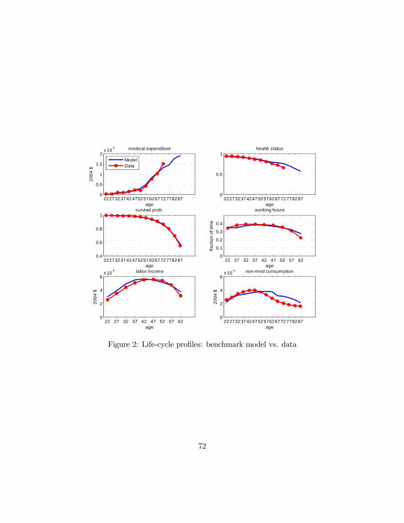
22273237424752576267727782870
0.5
1
1.5
2x 10 4
age
2004
$
medical expenditure
ModelData
22273237424752576267727782870
0.5
1
age
health status
22273237424752576267727782870.4
0.6
0.8
1
age
survival prob.
22 27 32 37 42 47 52 57 620
0.1
0.2
0.3
0.4
age
fract
ion
of ti
me
working hours
22 27 32 37 42 47 52 57 620
2
4
6x 10 4
age
2004
$
labor income
22273237424752576267727782870
2
4
6x 10 4
age
2004
$
nonmed consumption
Figure 2: Life-cycle profiles: benchmark model vs. data
72

22 27 32 37 42 47 52 57 62 67 72 77 82 870
0.5
1
1.5
2
2.5
3
3.5
4
4.5
age
CMotiveIMotiveSMotive
Figure 3: Life-cycle profiles of consumption, investment, and survival motive forhealth investment
73

22 27 32 37 42 47 52 57 62 67 72 77 82 870
0.2
0.4
0.6
0.8
1
1.2
1.4
1.6
1.8
2x 10 4
age
2004
$
BenchmarkNo CMotiveNo IMotiveNo SMotive
Figure 4: Life-cycle profile of medical expenditures: decomposition without recali-bration
74

22 27 32 37 42 47 52 57 62 67 72 77 82 870.2
0.4
0.6
0.8
1
age
health status
BenchmarkNo CMotiveNo IMotiveNo SMotive
22 27 32 37 42 47 52 57 62 67 72 77 82 870.5
0.6
0.7
0.8
0.9
1
age
survival prob.
Figure 5: Life-cycle profiles of health status and survival probability: decompositionwithout recalibration
75

22 27 32 37 42 47 52 57 62 67 72 77 82 870
0.2
0.4
0.6
0.8
1
1.2
1.4
1.6
1.8
2x 10 4
age
2004
$
BenchmarkNo CMotiveNo IMotiveNo SMotive
Figure 6: Life-cycle profiles of medical expenditure: decomposition with recalibration
76

22 27 32 37 42 47 52 57 62 67 72 77 82 870
0.5
1
1.5
2x 10 4
age
2004
$
medical expenditure
Benchmarkcoverage rate=0%coverage rate=40%
22 27 32 37 42 47 52 57 62 67 72 77 82 870.4
0.5
0.6
0.7
0.8
0.9
1
age
health status
Figure 7: Life-cycle profiles of medical expenditures and health status: reduce cov-erage rate
77

22 27 32 37 42 47 52 57 62 67 72 77 82 870
2
4
6
8
10
12x 10 4
age
2004
$
assets
22 27 32 37 42 47 52 57 62 67 72 77 82 871
2
3
4
5
6
7x 10 4
age
2004
$
total income
Benchmark (replace=40%)replace=0%replace=20%replace=60%
Figure 8: Life-cycle profiles of assets and total income: changing replacement ratio
78

22 27 32 37 42 47 52 57 62 67 72 77 82 870
0.5
1
1.5
2
2.5x 10 4
age
2004
$
medical expenditure
22 27 32 37 42 47 52 57 62 67 72 77 82 870.5
0.6
0.7
0.8
0.9
1
age
health status
Benchmark (replace=40%)replace=0replace=20%replace=60%
Figure 9: Life-cycle profiles of medical expenditures and health status: differentreplacement ratio
79

22 27 32 37 42 47 52 57 62 67 72 77 82 870
2
4
6x 10 4
age
2004
$
assets
22 27 32 37 42 47 52 57 62 67 72 77 82 870
0.5
1
1.5
2x 10 4
age
2004
$
medical expenditure
22 27 32 37 42 47 52 57 62 67 72 77 82 870.4
0.6
0.8
1
age
health status
BenchmarkDelay retirement
Figure 10: Life-cycle profiles of assets, medical expenditures and health status: de-laying retirement age
80

22 27 32 37 42 47 52 57 62 67 72 77 82 870
0.5
1
1.5
2x 10 4
age
2004
$
medical expenditure
22 27 32 37 42 47 52 57 62 67 72 77 82 870.5
0.6
0.7
0.8
0.9
1
age
health status
BenchmarkIncrease B 10%Increase B 20%
Figure 11: Life-cycle profiles of medical expenditures and health status: increase B
81