Embed Size (px)
Citation preview
May
2017
HEALTH CARE AND LIFE SATISFACTION IN SPAIN
AN EMPIRICAL ANALYSIS FOR THE PERIOD 2002 - 2014
Iban Ortuzar Fernández
Tutor: Angels Xabadia
1
Abstract
This document analyzes the effect of health care spending on the reported
level of satisfaction in Spain during the period 2002 - 2014. Using data from
the European Social Survey a panel data model is estimated for the 17 different
regions over the 7 waves of the survey. The results show that health care
spending per capita do have a positive effect on life satisfaction. Analyzing its
three main components separately, it turns out that only the expenditures on
pharmacy and primary health care seem to explain this effect. In addition, the
outcomes of the model also show that both higher levels of GDP growth and
GDP per capita tend to explain higher levels of satisfaction. Oddly enough,
unemployment and inflation also seem to be positively correlated. Finally,
some social characteristics also appear to explain some of these variations,
such as marital status and subjective perception of one´s health.
2
Contents
1. Introduction and objectives .......................................................................................... 3
2. Review of the research in happiness and literature: an overview ................................ 5
3. Descriptive analysis of the data ................................................................................... 9
3.1 Health care spending in Spain during the period 2002 – 2014 ............................. 9
3.2 Data on life satisfaction during the period 2002 – 2014 ..................................... 16
4. Methodology and results ............................................................................................ 21
4.1 Explanatory variables ......................................................................................... 21
4.2 The model specification ...................................................................................... 23
4.3 Results ................................................................................................................. 23
5. Conclusions ................................................................................................................ 28
6. References .................................................................................................................. 29
7. Appendices ................................................................................................................. 31
Appendix A ................................................................................................................. 31
Appendix B ................................................................................................................. 33
Appendix C ................................................................................................................. 34
Appendix D ................................................................................................................. 35
3
1. Introduction and objectives
There are two main health care models prevailing in Europe nowadays, one based
on mandatory quotas paid to the Social Security by employers and employees
(Bismarck model) and the other financed mostly by public taxes (Beveridge model).
While in the first one we can find countries like Germany, France or Belgium, the latter
is leaded by Denmark, Italy and Spain. In the Bismarck model (also known as Social
Health Insurance) the quotas collected are deposited in non-governmental funds
regulated by law that manage all the resources, arranging the different contracts with
hospitals, suppliers and employees. In the Beveridge model (aka National Health
Service) instead, the whole public health care system is financed by progressive taxes
and controlled by the state, which means that the total spending in health care is
accounted in the National Budget every year. Therefore, the actions of the Government
play a crucial role regarding the provision of health care services in the countries
applying the Beveridge model.
The health care system in Spain has been under the focus these last years, as it has
suffered a shortage of resources, first conducted by the crisis and then aggravated by the
adjustment plan launched in 2012 by the Spanish government. On balance, the depth
and duration of the crisis in Spain has had a clear negative effect on the welfare state
and especially on the provision of health care services, which are among the budget
items that have received greater cutbacks. The discomfort among the population has
been noticeable, as people have been demonstrating on the streets against these policies.
According to the National Barometer of Health, the satisfaction with the overall health
care system dropped throughout the crisis until reach a grade of 6.31 in 2014, compared
to the 6.59 given in 20111. The survey also reports that while in 2007 the health care
system was ranked the 10th concern among of the respondents, it had raised to the 5th
place in 20142. The motivation for this dissertation thus, lies on the study of whether
the average level of life satisfaction over time is affected or not by the health care
spending.
The objectives of this work can be divided as: (i) Study how the main
macroeconomic variables, which will be used as a control variables, have affected the
overall level of satisfaction in Spain during the period 2002-2014, and see if the results
1 G. Sevillano, Elena (2015). “Los usuarios dan a la sanidad pública su peor nota desde 2008”.
http://politica.elpais.com 2 Barómetro febrero 2014: http://datos.cis.es/pdf/Es3013mar_A.pdf
4
support the previous studies on life satisfaction. And (ii), analyze the specific effect of
the three main components of the public health care spending in Spain: hospital and
specialized health care, pharmacy and primary health care. Since Spain is a country in
which people rely mostly on the provision of the health care services by the State, we
should expect a positive relationship between the quantity of money spent in health care
services and life satisfaction. And of the three main components, primary health care
probably is the one which have more effect, since it is the provision at a local level and
what can be more directly observed by individuals. Therefore, the hypothesis to
formulate here can be state as: Health care spending has a positive effect on life
satisfaction, and we can expect the primary health care component being the one with a
larger impact.
This document is structured as follows: Chapter 2 makes an overview of the
economic research in happiness and points out the main findings in this field. Chapter 3
presents the evolution of the health care spending in Spain, both national and regional,
and its corresponding evolution of the levels of satisfaction during the period. Chapter 4
explains the methodology as well as the main variables used, and presents the
econometric results and its analysis. Finally, chapter 5 ends with the main conclusions
drawn from this document.
5
2. Review of the research in happiness and literature: an overview
Over the last years, the interest for the analysis of the subjective well-being has
increased significantly among economists. This new approach challenges the former
objectivist theory of the utility, which is based on choices made by individuals (revealed
preferences). According to this view, these decisions and choices provide all the
information needed to value individual’s level of utility. The new subjectivist approach
instead, takes into account the wide range of beliefs that people have about what
happiness and quality of life actually is, pointing out that the observed behavior is just
an incomplete indicator of individual’s level of welfare. Therefore, the assumption
made here is that people are, in fact, the best judges of their own quality of life. Surveys
that ask directly to individuals about how satisfied are them with their quality of life or
level of happiness, according to their personal circumstances or experiences, enable us
to treat this data as empirical approximations of the individuals level of utility
(Veenhoven, 1984). The terms usually used to describe subjective well-being are life
satisfaction and happiness. Life satisfaction is usually asked as: “Taking all things
together how satisfied are you with your life as a whole nowadays?”, with an ordinal
answer. Therefore, when we talk about life satisfaction we are assuming cognitive
judgments about how people feel their life as a whole. Happiness on the other hand,
answers the question: “How happy are you?”, giving an emotional response that
measures people’s current feelings (Clark and Senik, 2011). Both terms are the main
components of the overall subjective well-being, which can be defined as ‘a person’s
cognitive and affective evaluations of his or her life’ (Diener, Lucas, & Oshi, (2002), p.
63)3.
Today, the measurement of subjective well-being is increasingly gaining a lot of
attention, not only among researches but also among politicians. Trying to measure and
understand what drives people’s level of happiness or life satisfaction is becoming one
of the main goals in social sciences, especially in developed countries. Against what it
was believed in the past, the reported level of subjective well-being is not as directly
related as it was thought with income (Easterlin, 1974). This suggests thus, that instead
of focusing only on the performance of the main economic indicators such as the GDP
growth, level of inflation or level of unemployment, policymakers should also
3 Despite the technical differences between the terms, subjective well-being, life satisfaction and
happiness are used as synonyms throughout the document
6
concentrate on those policies that may affect the subjective level of well-being, which,
in turns, can contribute to other important outcomes such as productivity (Oswald, Proto
and Sgroi, 2014) or better health (Siahpush (2008) and Veenhoven (2008b)).
The need to incorporate this new dimension into the indicators of economic
progress has raised a lot of initiatives during the beginning of this century. In 2005, and
inspired by the philosophy of the Bhutan’s Kingdom, the International Institute of
Management (U.S.) launched the Gross National Happiness index (GNH)4, also known
as the Gross National Well-being (GNW), which was the first of its kind combining
subjective measures (satisfaction) and objective data (economic indicators), tracking 7
different areas of wellness. This index set the first framework for future research
combining both subjective and objective data, going one step further compared to others
development indexes that already went beyond the simple measure of the GDP (e.g.
HDI). In 2008 the French president Nicolas Sarcozy, assessed by two Nobel Prizes5
under the name ‘The Quality life Comission’, announced a revolutionary plan to include
happiness and well-being among the key indicators of economic progress6. According
to him, the standard measures of growth ignore some other factors vital to the well-
being of the population: "GDP statistics were introduced to measure market economic
activity. But they are increasingly thought of as a measure of societal well-being, which
they are not." A year later, and because of the success of the initial conference in 2007,
the European Commission released its own road map under the initiative ‘GDP and
beyond’7. Most recently, in 2011, the OECD released the Better Life Index (BLI) along
with the report “How is life?”. This index covers 40 countries, including all OECD
members, and analyzes the situation of 11 different social areas, such as living
conditions, provision of public services, work-life balance or life satisfaction. The next
year, the United Nations released the ‘World Happiness Report’, a global survey that
scores and ranks 156 countries by their level of happiness. Many other initiatives have
been launched at a national level by different countries; all of them aimed to measure
and include happiness in their measurement of national wealth8.
4 See disambiguation with the GNH Bhutan index (1972): http://gnh.institute/gnh-index-gnw-index/gnh-
vs-gnw-gnh-2.htm 5 Joseph Stiglitz (2001) and Armatya Sen (1998)
6 Samuel, H. (2009) “Nicolas Sarkozy wants to measure economic success in 'happiness'“
http://www.telegraph.co.uk 7 See http://ec.europa.eu/environment/beyond_gdp/background_en.html for more detailed information
8 To see the full timeline: http://gnh.institute/happiness-economics/happiness-economics-timeline-
milestones-history.htm
7
The economic research in happiness has provided many important insights so far,
pointing out some key determinants of the subjective well-being. Easterlin (1974, 1995,
2001) found that income growth did not correlate as close as it was expected with the
individual’s level of satisfaction, stating that even though the richer individuals within a
society tend to report highest levels of satisfaction, this did not hold at a country level.
This, also known as the ‘Easterlin paradox´, basically meant that continuous increases
in the level of real per capita income did not led to higher levels of satisfaction in a
country. Veenhoven (2003) did not find evidence of the paradox. Later on, Stevenson
and Wolfers (2008) reconsidered the ´Easterlin paradox´, concluding that subjective
well-being increases but slowly than real per capita income does. Oswald (1997) found
that for US satisfaction seems to rise as the real income does, but that the contribution is
so small that sometimes difficult to detect. Oswald (1997) also said that governments
should first fight the amount of joblessness in the economy since unemployment seems
to be a larger source of unhappiness. Di Tella, MacCulloch and Oswald (2003) showed
that macroeconomic fluctuations have a noticeable effect on the overall level of
happiness of nations. After controlling for a wide range of personal and regional
characteristics, they found that the level of subjective well-being stands significantly
correlated with both the level and change in GDP per capita, the rates of inflation and
unemployment, and that there is constant gap between employed and unemployed
people. Di Tella et al (2003) also found that cost of recessions were large, since the fall
in the level of happiness during these periods extended beyond the decline of those
macroeconomic variables. Welsch and Kühling (2015) analyzed, from data of 25 OECD
countries, how the crisis of 2008 - 2009 had affected the subjective well-being. They
conclude that GDP growth, level of unemployment and inflation do affect the overall
level of satisfaction, being the first the one that has more impact. Using data for Spain,
which is the same case of this thesis, Gamero (2009) found that, in contrast to previous
studies treating macroeconomic variables, the level of unemployment and inflation had
a positive effect on happiness in Spain, for the period 1999-2004. He attributes these
results to a ‘comparative effect’ for the case of unemployment9: employed people value
more their situation when unemployment is high in the region in which they belong; and
a ‘monetary illusion’ for the case of inflation: people do feel richer when see their
wages increase, even though that does not mean an increase in the purchasing power.
9 Unemployed people are not included in this study. Therefore, these results could be different in their
case.
8
Some other studies analyze the relationship between individuals’ own satisfaction
and the level of income of a reference group (see e.g. Ferrer-i-Carbonell (2004) or
Georgellis, Tsitsianis and Ping Yin (2009)), showing a negative correlation between the
increase in income of the reference group and one’s level of well-being. Other paths of
research have also focused on how life satisfaction responds to environmental and
quality life conditions, also externalities. Higher levels of both noise and poor air
quality at the workplace tend to reduce significantly the level of satisfaction (See e.g
García-Mainar, Montuenga and Navarro-Paniagua (2015) or Ferreira, Akay and
Brereton (2013)).
Less research has been carried out as far as the provision of public goods or the
size of the welfare state is concerned, especially for the case of healthcare services. On
the one hand, Veenhoven (2000), using large data of 40 countries for the period 1980-
1990, finds no relation between the size of welfare state and the level of satisfaction. On
the other, Bjornskov, Dreher and Fischer (2007) conclude that satisfaction decreases as
government spending increases. Likewise, using data from the European Social Survey
covering the years 2002-2006 Bollerman (2009) does find a negative correlation
between the average level of happiness and the welfare state spending. These studies
though, only measure the aggregate expenditures of the state and not any specific
provision of public service, which is what individuals can observe and therefore affect
their level of happiness. In this sense, Di Tella et al. (2003) did find a positive
relationship between the level of satisfaction and the income replacement rate10
and
unemployment benefits for unemployed people. Regarding the provision of health care
services, Kotakorpi and Laamanen (2007) found that excess expenditure in primary
health care have a positive effect on happiness, whereas the spending on specialized
health care does not. However, this study only analyzes the data of one single year
(2000) and do not take into account the main macroeconomic indicators. To my
knowledge, this is the only research studying the relationship between health care
services and life satisfaction.
10
The percentage of working income that must be paid out a pension fund for retirement
9
3. Descriptive analysis of the data
3.1 Health care spending in Spain during the period 2002 – 2014
To begin with, the health care system in Spain is not bad, but rather the opposite.
Spain possesses one of the most generous and efficient systems in the world, giving
coverage to the entire population regardless of their labor status or nationality. Health
care in Spain is completely free and universal, and is one of the few countries (together
with Denmark and United Kingdom) that only apply a copayment for prescription
medicines. In the most of the other countries, the copayment is extended to all the other
health care services (including primary health care and hospital and specialized health
care). The effectiveness of the system is reflected on the health indicators, which are
above the European average, and some at the head (e.g. highest life expectancy at birth
or the second lowest rate of mortality11
). Spain was ranked 7th
in the ranking published
by the World Health Organization in their report in 2000, which evaluated 191 different
countries regarding the average level of population’s health (50%), quick response of
the health services (25%) and fairness in financing the health care system (25%)12
.
However, the health care system in Spain has gone through tough times these last years,
not only has been affected by the crisis, but also for the adjustment plan launched in
2012 by the Spanish government. The plan, whose main objective was to restore the
budget deficit and align it to the European fiscal pact (signed in 2012), applied austerity
measures to all the budget items, and expecting to reduce the yearly health care and
education spending in 10000 M€.
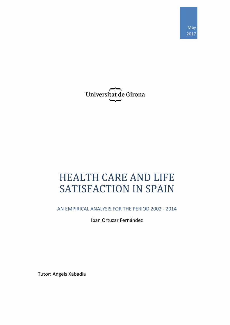
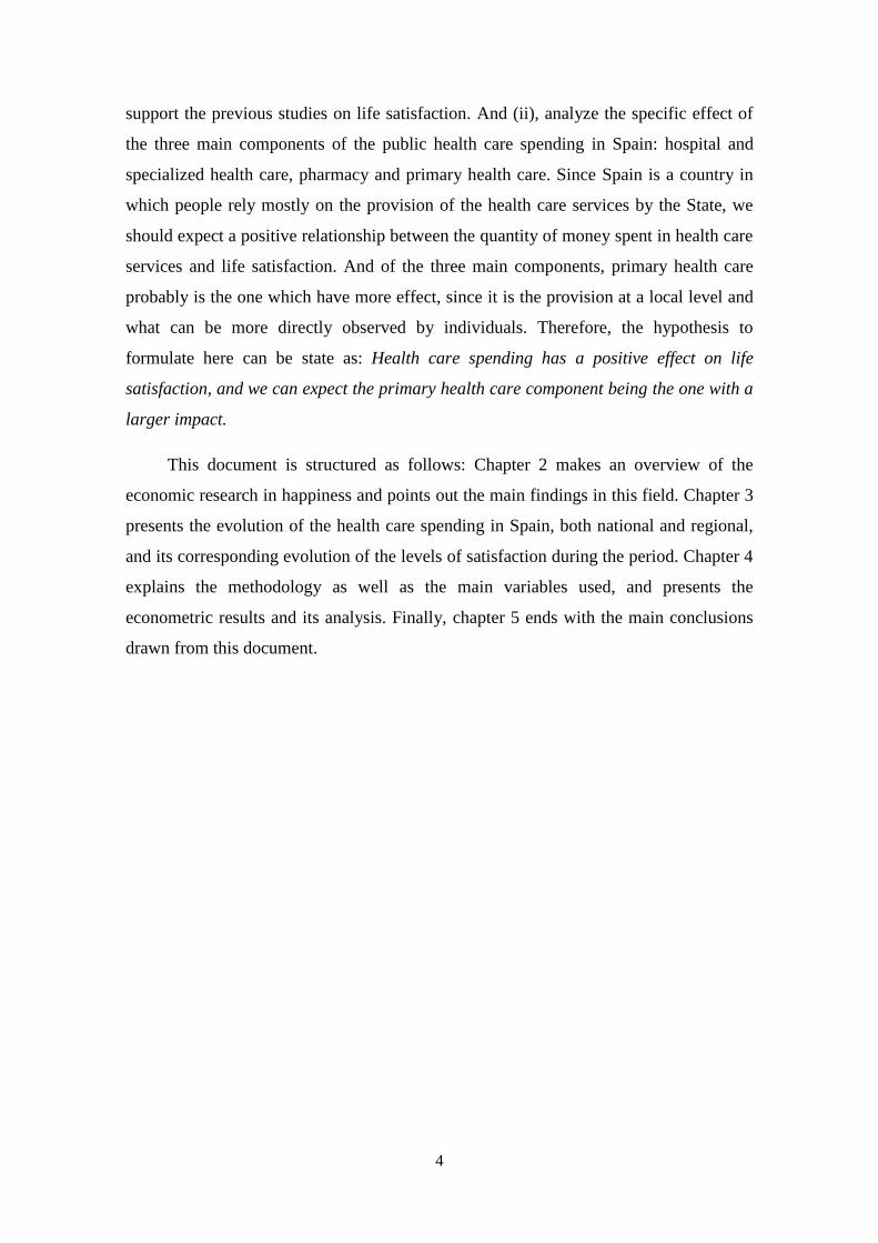
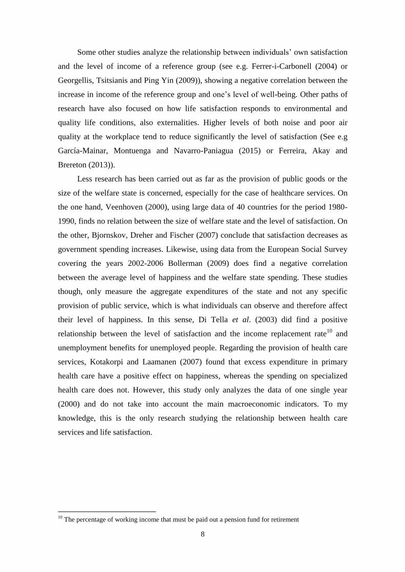
The total health care spending in Spain has been following a positive trend since
2000, rising along with the GDP growth during this period. As we can see in figure 1, in
2009 the total money spent in public health care accounted for 70.560 million of Euros
compared to the 38.552 of 2002. As a percentage of the GDP, the health care system has
always represented around the 5 – 7%, reaching the highest rate in 2009. Despite the
beginning of the crisis in 2008 the total spending on health care still raised the following
11
Spain health statistics:
https://www.msssi.gob.es/estadEstudios/estadisticas/inforRecopilaciones/indicadoresSalud.htm 12
The WHO declined to rank again the different countries the following years because of the controversy
and the criticism raised with the methodology used. Many other rankings have been launched by private
organizations later on, such as Bloomberg (Bloomberg Health Care-efficient index, which ranked Spain
3rd
in 2015) or the Health Consumer Powerhouse (Euro health consumer index, which ranked Spain in the
19th
position respect 35 European countries in 2015). Obviously, not free of criticisms.
10
year. However, since 2010 the total spending started to fall until reach the lowest level
in 2013, when it accounted for 61.760 million of euros.
Figure 1. Evolution of the total health care spending and its share of the GDP
Source: Own elaboration based on data from the Ministry of Health and the National Institute
of Statistics (INE)
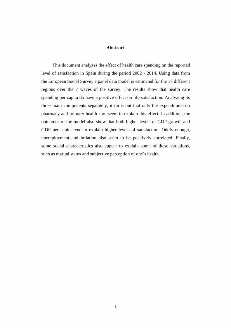
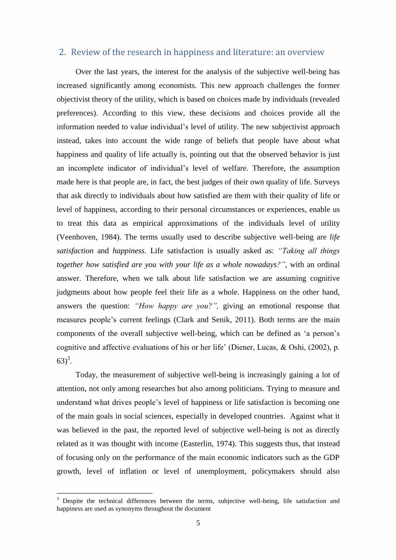
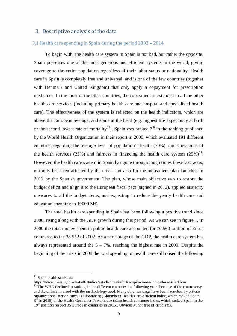
Observing figure 2 we can see that the crisis had a negative effect on the total
health care spending, even though with a lagged effect. After an increase of 5.6% in
2008/09 respect to the previous year, this fell by 1.6% and 2 % the year 2010 and 2011
respectively. However, we can see that since the year 2012, when the Spanish
government announced the adjustment plan, the decrease in total health care spending
was significantly affected, being reduced much more than the fall in the GDP. This
situation was held the subsequent year, accounting with a reduction of the 3.8% respect
of the year 2012, and with a lower increase in 2014 when the GDP growth was already
recovering. This period, first conducted by the crisis and aggravated by the fiscal
consolidation put under pressure the financing of the public health services, reducing in
nominal terms 8800 M€ of the annual budget between 2009 (the year with the highest
expenditure) and 2014 (when it stopped falling).
5,1% 5,3% 5,4% 5,4% 5,5% 6,2% 6,0%
6,5% 6,4% 6,4% 6,2% 6,0% 6,0%
0,0%
2,0%
4,0%
6,0%
8,0%
10,0%
12,0%
14,0%
16,0%
18,0%
25000
30000
35000
40000
45000
50000
55000
60000
65000
70000
75000
2002 2003 2004 2005 2006 2007 2008 2009 2010 2011 2012 2013 2014
HCS as a percentatge of the GDP Total healt care spending (Million of €)
11
Figure 2. Interannual variation of total public spending on health care services and GDP
growth
Source: Own elaboration based on data from the Ministry of Health and the National
Institute of Statistics (INE)
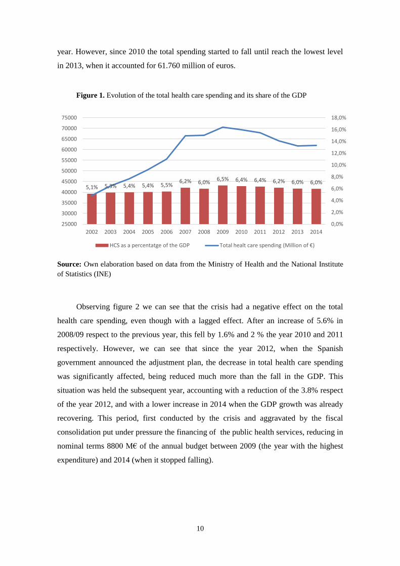
Table 1 shows the distribution of the health care budget of a representative year (2014)
according to the functional classification. As we can appreciate, there are three components that
represent more than the 90% of the total budget, which are hospital and specialized health care,
pharmacy (prescriptions) and primary health care (local and primary services). By far, the first
is the one that represents a greater share of the total health care budget, with a 61.4% for the
year 2014.
Table 1. Representative year of the national total health care budget according to the
functional classification
2014
Total spending (M€) Percentage
Hospital and specialized services 38.042,703 61,4%
Pharmacy 10.388,440 16,8% 92,8%
Primary health care 9.045,442 14,6%
Capital spending 862,227 1,4%
Collective services 1.720,151 2,8%
Prostheses and therapeutic devices 1.235,571 2,0%
Public health care 652,508 1,1%
0,3%
5,6%
-1,6% -2,0%
-5,7%
-3,8%
0,4% 1,1%
-3,6%
0,0%
-1,0%
-2,9%
-1,7%
1,4%
-8%
-6%
-4%
-2%
0%
2%
4%
6%
8%
07/08 08/09 09/10 10/11 11/12 12/13 13/14
Total health care spending GDP
12
Total 61.947,041
Source: Own elaboration based on data from the Ministry of Health.
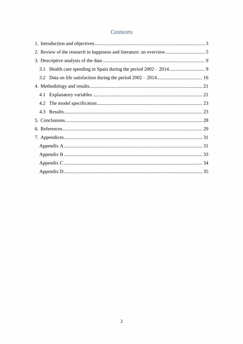
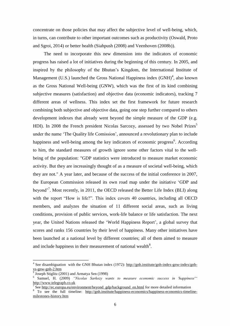
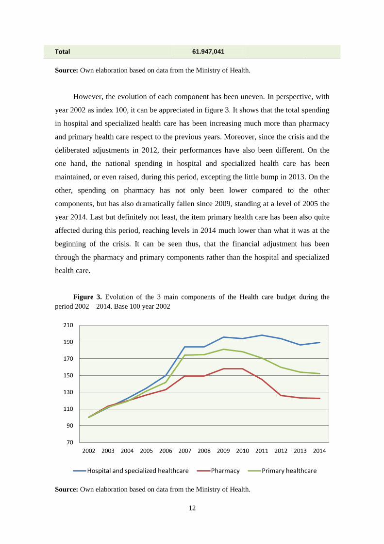
However, the evolution of each component has been uneven. In perspective, with
year 2002 as index 100, it can be appreciated in figure 3. It shows that the total spending
in hospital and specialized health care has been increasing much more than pharmacy
and primary health care respect to the previous years. Moreover, since the crisis and the
deliberated adjustments in 2012, their performances have also been different. On the
one hand, the national spending in hospital and specialized health care has been
maintained, or even raised, during this period, excepting the little bump in 2013. On the
other, spending on pharmacy has not only been lower compared to the other
components, but has also dramatically fallen since 2009, standing at a level of 2005 the
year 2014. Last but definitely not least, the item primary health care has been also quite
affected during this period, reaching levels in 2014 much lower than what it was at the
beginning of the crisis. It can be seen thus, that the financial adjustment has been
through the pharmacy and primary components rather than the hospital and specialized
health care.
Figure 3. Evolution of the 3 main components of the Health care budget during the
period 2002 – 2014. Base 100 year 2002
Source: Own elaboration based on data from the Ministry of Health.
70
90
110
130
150
170
190
210
2002 2003 2004 2005 2006 2007 2008 2009 2010 2011 2012 2013 2014
Hospital and specialized healthcare Pharmacy Primary healthcare
13
Nevertheless, Spain is a highly decentralized country, which has transferred most
of its competences to its regions, also known as Autonomous Communities. And the
health care competence is not an exception13
. The health care system in Spain is divided
into 17 different sub-divisions (each one managed by every region). All of them
controlled by the National Health System's Inter-territorial Council, whose aim is to
promote the coordination, cooperation and communication among regions and the
central administration and ensure the quality and equity of the health care services of the
citizens around the country. According to the Constitution and the article 41 of the
General Health Act every region is able to apply its competences according to its own
Statute of autonomy, unless some decisions or actions have been reserved to the central
government. This basically means that, even though the central government is the
responsible for collecting taxes, every community can decide where to spend and invest
the money that is returned according to the distribution criteria. This is a very important
issue to take into account when analyzing the situation of Spain, since every region can
behave very different in response of their economic situation or even for cultural or
social disparities.
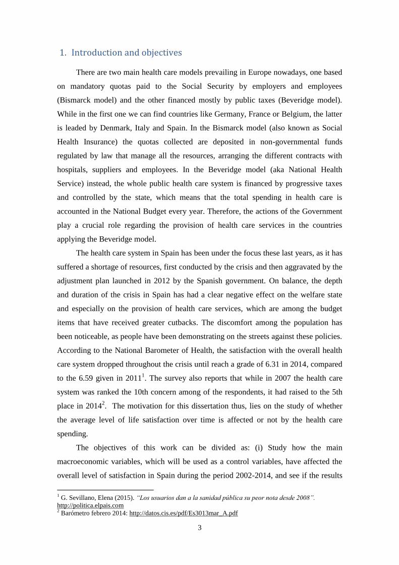
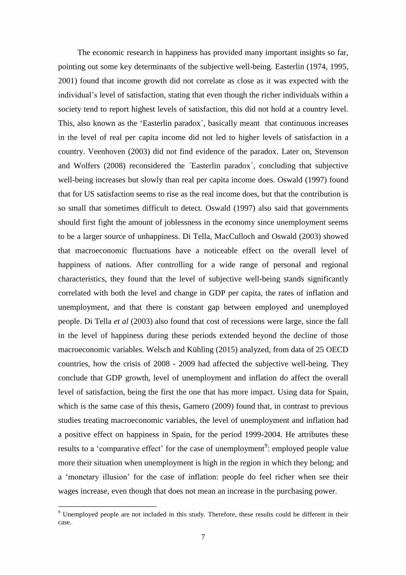
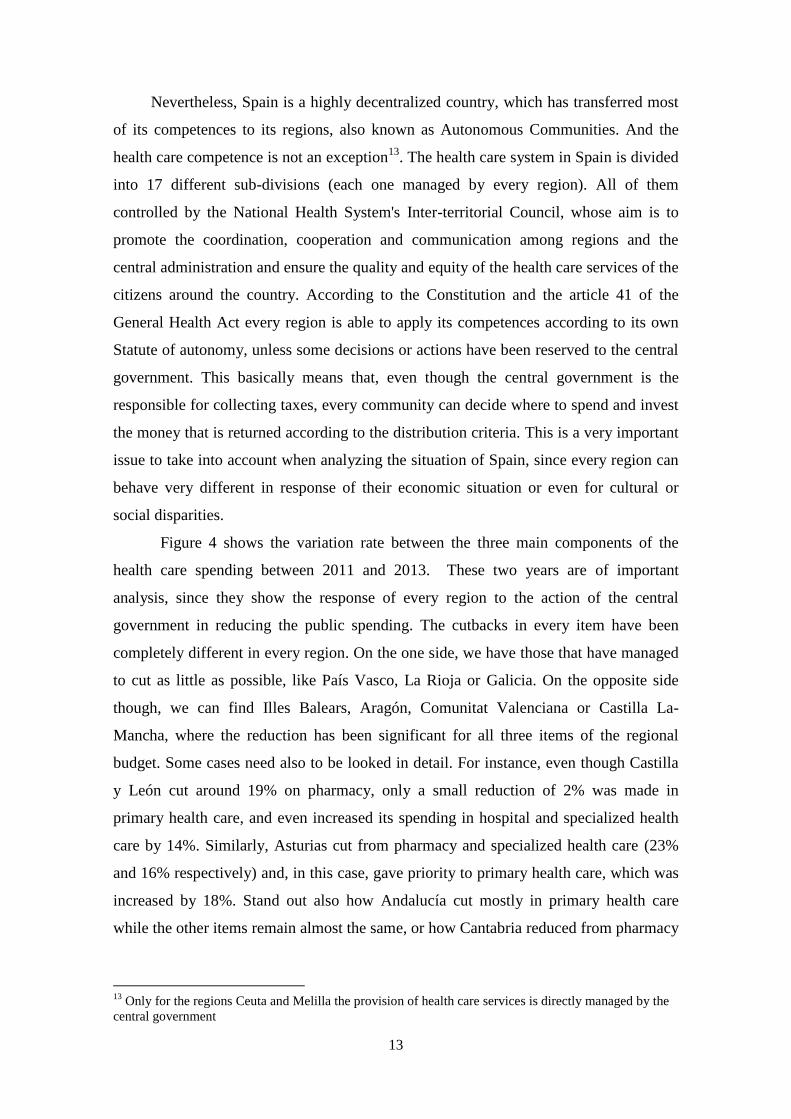
Figure 4 shows the variation rate between the three main components of the
health care spending between 2011 and 2013. These two years are of important
analysis, since they show the response of every region to the action of the central
government in reducing the public spending. The cutbacks in every item have been
completely different in every region. On the one side, we have those that have managed
to cut as little as possible, like País Vasco, La Rioja or Galicia. On the opposite side
though, we can find Illes Balears, Aragón, Comunitat Valenciana or Castilla La-
Mancha, where the reduction has been significant for all three items of the regional
budget. Some cases need also to be looked in detail. For instance, even though Castilla
y León cut around 19% on pharmacy, only a small reduction of 2% was made in
primary health care, and even increased its spending in hospital and specialized health
care by 14%. Similarly, Asturias cut from pharmacy and specialized health care (23%
and 16% respectively) and, in this case, gave priority to primary health care, which was
increased by 18%. Stand out also how Andalucía cut mostly in primary health care
while the other items remain almost the same, or how Cantabria reduced from pharmacy
13
Only for the regions Ceuta and Melilla the provision of health care services is directly managed by the
central government
14
and increased specialized health care while did not touch the primary health care
spending at all.
Figure 4. Variation rate between 2011 and 2013 of the 3 main components of the health
care budget by region
Source: Own elaboration based on data from the Ministry of Health.
In aggregate terms, we can see that the total health care spending per capita also
differs by region. Figure 5 and 6 show the total spending in public health care per
capita of the different regions for the years 2009 and for the 2014 respectively. By 2009,
which was the year with the higher national amount spent in health care with 70560 M€,
the region with the higher spending per capita was País Vasco with 1656,7 €. The
lower, was Andalucía with 1246,6 €, and the mean was set in 1521,8 €. In 2014, things
had substantially changed. The healthcare spending per capita of all the regions had
decreased compared to 2009 levels. País Vasco still was at the head with a decline of
4,6% respect to 2009 whereas Andalucía was the lower with a reduction of 19,7%. The
average was also decreased to 1333,5 €. Notice that in 2014 almost all the regions
remain in the same relative position compared to 2009. Only Cantabria avoided cutting
as much as the others did, and even managed to increase its spending per capita
standing above the average.
-80,0% -60,0% -40,0% -20,0% 0,0% 20,0% 40,0%
ANDALUCÍA
ARAGÓN
ASTURIAS
ILLES BALEARS
CANTABRIA
CANARIAS
CATALUÑA
CASTILLA Y LEÓN
CASTILLA LA MANCHA
VALENCIA
EXTREMADURA
GALICIA
MADRID
MÚRCIA
NAVARRA
PAÍS VASCO
LA RIOJA
Hospital and specialized healthcare Pharmacy Primary health care

15
Figure 5. Health care spending per capita per region in year 2009
Source: Own elaboration based on data from the Ministry of Health
Figure 6. Health care spending per capita per region in year 2014
Source: Own elaboration based on data from the Ministry of Health
1246,4
1384,2
1521,8
1656,7
0 500 1000 1500 2000
ANDALUCIA
MADRID
ILLES BALEARS
VALENCIA
CANTABRIA
CASTILLA Y LEON
CATALUÑA
LA RIOJA
GALICIA
CANARIAS
Mean
CASTILLA LA MANCHA
ARAGON
MURCIA
EXTREMADURA
NAVARRA
ASTURIAS
PAIS VASCO
1041,3
1333,5
1409,1
1583,9
0 500 1000 1500 2000
ANDALUCIA
MADRID
ILLES BALEARS
VALENCIA
CASTILLA LA MANCHA
CANARIAS
CATALUÑA
CASTILLA Y LEON
GALICIA
Mean
LA RIOJA
CANTABRIA
MURCIA
ARAGON
NAVARRA
ASTURIAS
EXTREMADURA
PAIS VASCO
16
3.2 Data on life satisfaction during the period 2002 – 2014
The data used for the analysis of the subjective well-being has been extracted
from the European Social Survey (ESS)14
, a survey carried out every two years since
2002. The questions asked cover a large range of topics, which go from individual and
personal characteristics such as social life, labor status or subjective well-being, to
topics regarding country issues, such as trust in the legal systems, politics or
immigration. Regarding subjective well-being, two questions are asked: “taking all
things together, how happy would you say you are?” and “All things considered, how
satisfied are you with your life as a whole nowadays?” . For both questions, the
respondents must answer a number within the scale 0-10, where 0 means “extremely
unhappy/dissatisfied” and 10 “extremely happy/satisfied”. There are more than 30
participating countries, including all the European ones. For every round, samples are
randomly selected, and every individual is personally interviewed. Moreover, the data is
not only at a national level but also at three different regional levels, NUTS 1, 2 and 315
.
So far, seven rounds have been carried out 16
and the data is freely available on its
database.
For the case of Spain, all 7 rounds (covering the years 2002/4/6/8/10/12/14) are
available at a NUT 2 level, which corresponds to the Autonomous Community region.
Between the two questions on subjective well-being, the variable chosen is satisfaction
with life. Since the purpose here is to analyze the relationship between health care
spending and subjective well-being of people, we expect cognitive judgments about
how people feel their life as a whole regardless of their emotions or feelings. A total of
12993 valid cases are collected throughout the 7 rounds, with the following distribution
per year:
Table 2. Number of respondents by round
2002 2004 2006 2008 2010 2012 2014 Total
Respondents 1567 1566 1831 2492 1857 1822 1858 12993
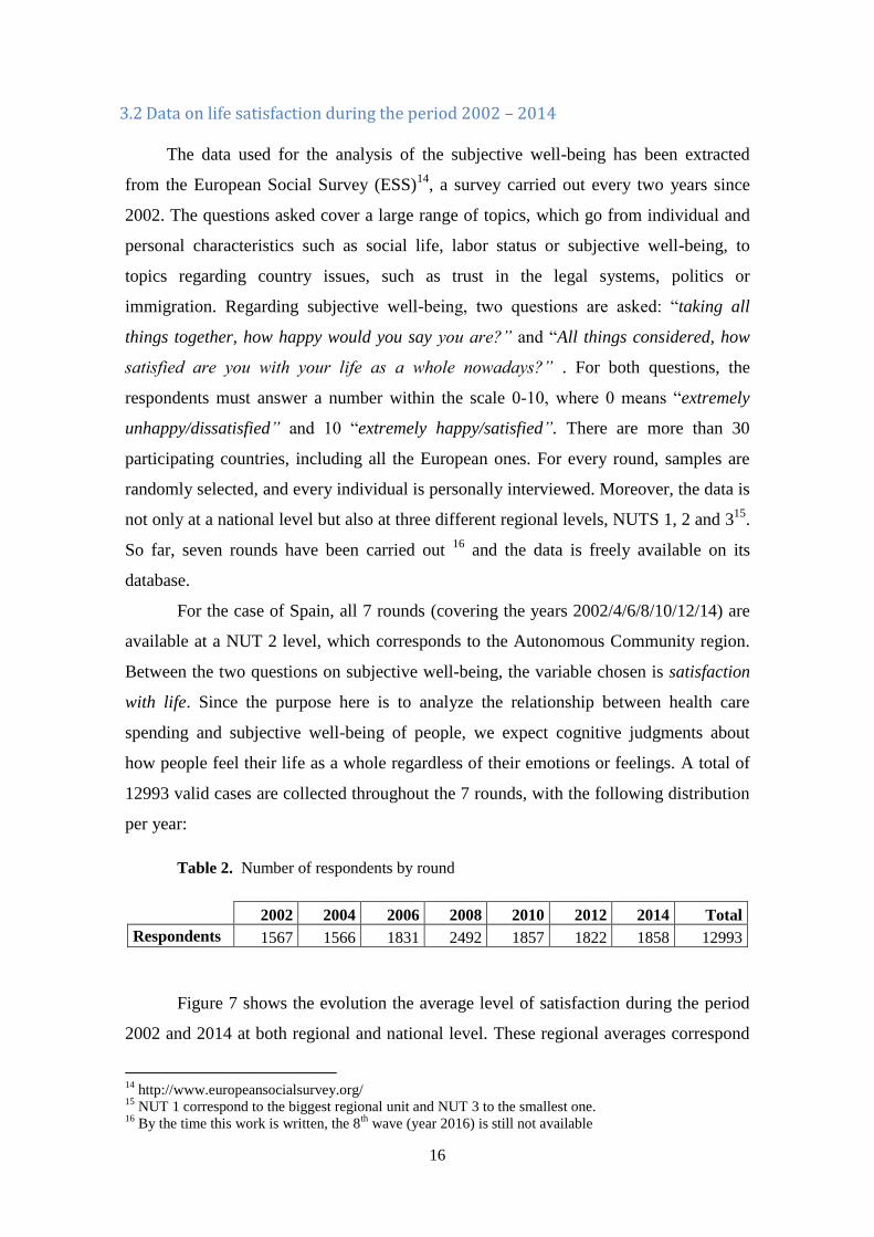
Figure 7 shows the evolution the average level of satisfaction during the period
2002 and 2014 at both regional and national level. These regional averages correspond
14
http://www.europeansocialsurvey.org/ 15
NUT 1 correspond to the biggest regional unit and NUT 3 to the smallest one. 16
By the time this work is written, the 8th
wave (year 2016) is still not available

17
to the mean of the sample of every region for every year, while the national average is
the mean of the all 17 regions per year. As it can be appreciated, the Spanish average
level of satisfaction noticeably raised up during the period 2002 – 2006, reaching up to
a grade of 7,44 this last year compared to 2002, when it was a grade of 6,91. Also of
interest, is to see how the means of the all regions converge in 2006. The region with
the lowest average stood at the threshold of the grade 7 and at closely the 8 threshold
the region with the highest valuation. By the beginning of the crisis, the 2008 levels
show that the national average slightly fell, waning to a mean of 7,26. The regional
levels diverged again that year, with a big difference between the highest region (7,78)
and the lowest (6,62) . In 2010, the average levels went up again, getting almost the
same grades that in 2006. However, in 2012 there was the sharpest decrease of the
whole period, standing the national average at a 6,96. For the next round (2014), the
average slightly increased again, even though the regions’ means spread again.
Figure 7. Evolution of the average level of satisfaction (national and regional)
Source: Own elaboration based on data from the European Social Survey (ESS)
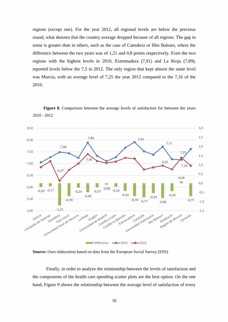
The year 2012 must be looked closely, not only because it registered the
strongest drop of the period, but also because it happened 4 years later after the
beginning of the crisis. Figure 8 shows the different regional levels for the years 2010
and 2012. Clearly, the average level of satisfaction between 2010 and 2012 fell in all
5
5,5
6
6,5
7
7,5
8
8,5
2000 2002 2004 2006 2008 2010 2012 2014 2016
Happiness National average
18
regions (except one). For the year 2012, all regional levels are below the previous
round, what denotes that the country average dropped because of all regions. The gap in
some is greater than in others, such as the case of Cantabria or Illes Balears, where the
difference between the two years was of 1,21 and 0,8 points respectively. Even the two
regions with the highest levels in 2010, Extremadura (7,91) and La Rioja (7,89),
reported levels below the 7,5 in 2012. The only region that kept almost the same level
was Murcia, with an average level of 7,25 the year 2012 compared to the 7,16 of the
2010.
Figure 8. Comparison between the average levels of satisfaction for between the years
2010 - 2012
Source: Own elaboration based on data from the European Social Survey (ESS)
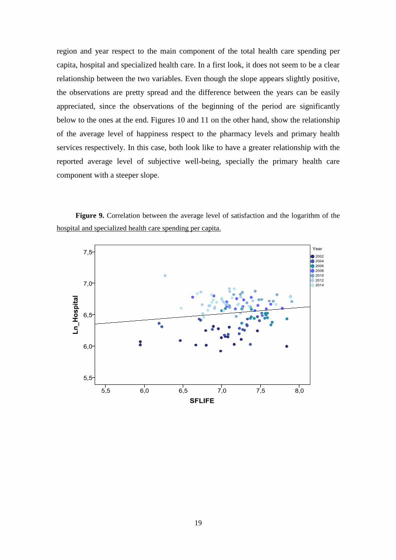
Finally, in order to analyze the relationship between the levels of satisfaction and
the components of the health care spending scatter plots are the best option. On the one
hand, Figure 9 shows the relationship between the average level of satisfaction of every
-0,20 -0,17
-1,21
-0,70
-0,24
-0,49
-0,22 -0,08
-0,19
-0,42
-0,70 -0,77 -0,54
-0,80
-0,43
0,09
-0,71
7,48
7,89 7,91 7,71
7,16
6,27
7,40 6,91
7,25
-1,5
-1,0
-0,5
0,0
0,5
1,0
1,5
2,0
2,5
3,0
5,00
5,50
6,00
6,50
7,00
7,50
8,00
8,50
Difference 2010 2012
19
region and year respect to the main component of the total health care spending per
capita, hospital and specialized health care. In a first look, it does not seem to be a clear
relationship between the two variables. Even though the slope appears slightly positive,
the observations are pretty spread and the difference between the years can be easily
appreciated, since the observations of the beginning of the period are significantly
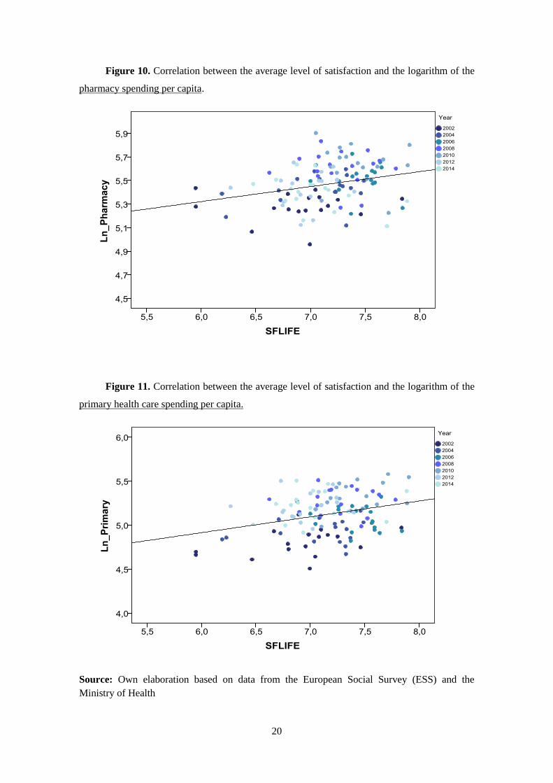
below to the ones at the end. Figures 10 and 11 on the other hand, show the relationship
of the average level of happiness respect to the pharmacy levels and primary health
services respectively. In this case, both look like to have a greater relationship with the
reported average level of subjective well-being, specially the primary health care
component with a steeper slope.
Figure 9. Correlation between the average level of satisfaction and the logarithm of the
hospital and specialized health care spending per capita.
20
Figure 10. Correlation between the average level of satisfaction and the logarithm of the
pharmacy spending per capita.
Figure 11. Correlation between the average level of satisfaction and the logarithm of the
primary health care spending per capita.
Source: Own elaboration based on data from the European Social Survey (ESS) and the
Ministry of Health
21
4. Methodology and results
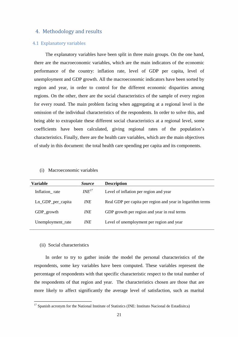
4.1 Explanatory variables
The explanatory variables have been split in three main groups. On the one hand,
there are the macroeconomic variables, which are the main indicators of the economic
performance of the country: inflation rate, level of GDP per capita, level of
unemployment and GDP growth. All the macroeconomic indicators have been sorted by
region and year, in order to control for the different economic disparities among
regions. On the other, there are the social characteristics of the sample of every region
for every round. The main problem facing when aggregating at a regional level is the
omission of the individual characteristics of the respondents. In order to solve this, and
being able to extrapolate these different social characteristics at a regional level, some
coefficients have been calculated, giving regional rates of the population’s
characteristics. Finally, there are the health care variables, which are the main objectives
of study in this document: the total health care spending per capita and its components.
(i) Macroeconomic variables
Variable Source Description
Inflation_ rate INE17
Level of inflation per region and year
Ln_GDP_per_capita INE
Real GDP per capita per region and year in logarithm terms
GDP_growth INE
GDP growth per region and year in real terms
Unemployment_rate INE
Level of unemployment per region and year
(ii) Social characteristics
In order to try to gather inside the model the personal characteristics of the
respondents, some key variables have been computed. These variables represent the
percentage of respondents with that specific characteristic respect to the total number of
the respondents of that region and year. The characteristics chosen are those that are
more likely to affect significantly the average level of satisfaction, such as marital
17
Spanish acronym for the National Institute of Statistics (INE: Instituto Nacional de Estadísitca)

22
status, level of studies, subjective perception of one´s health and gender. These
variables give regional rates for every round and for every social characteristic.
, such that k ≤ N (1)
Where:
s is the social characteristic
k is the number of respondents with that characteristic of the region i in the round t
N is the number of the sample of the region i in the round t
Variable Source Description
Div_Wid_Sep ESS18
Percentage of respondents that their marital status correspond
to widowed/divorced/separated. (The possible answers of the
question are: Married, Widowed, Divorced, Separated,
Single)
University_education ESS Percentage of respondents with university studies. Here are
included those with a bachelor’s degree or higher. (The
categories defined in the question are: Master or higher,
Bachelor’s degree, Post-secondary education, secondary
education and primary education)
Good_perception ESS Percentage of respondents that have a good perception of
their own health. Here are included those who reported: Very
good and Good. (The all answers of the questions are: Very
good, Good, Fair, Bad, Very bad)
Male ESS Percentage of respondents that are male
(iii) Health care variables
Variable Source Description
Ln_Health_spending MSSSI
19 Total spending on health care per capita (per region and year)
in logarithm terms
Ln_Hospitals MSSSI Health care spending per capita on hospital and specialized
services (per region and year) in logarithms terms
18
European Social Survey 19
Spanish acronym for the Ministry of Health (MSSSI: Ministerio de Sanidad, Servicios Sociales e
Igualdad)

23
Ln_Pharmacy MSSSI Health care spending per capita on pharmacy (per region and
year) in logarithms terms
Ln_Primary MSSSI Health care spending per capita on primary health care (per
region and year) in logarithms terms
4.2 The model specification
The multiple regression analysis is the method used in this document, where a
range of independent variables give response to the variations of the dependent variable
Life Satisfaction, which varies in a scale from 0 (the lowest level) to 10 (the highest).
Therefore, the equation to run here can be expressed as:
(2)
Where is the average level of satisfaction of the region i in the round t,
and is the vector of the different macroeconomic variables m observed for the
region i in the year t, the vector of the different social characteristics s
calculated for the region i in the year t, and the vector of the different health
care variables h for the region i in the year t. Finally, every β represent the different
coefficients for every independent variable, and uit the error term for region i and year t.
Taking advantage of the panel data, the model performed is a mixed model with fixed
and random effects. The random effect gathers the regional characteristic, while the rest
of explanatory variables are specified as fixed effects.
4.3 Results
Table 3 shows the econometric results of the equation (2). Model 1 only takes into
account the macroeconomic group of variables, in order to have a first glance of the
effects of the main economic indicators. In model 2, has been included the social group
characteristic, which contains the different individual characteristics collected on the
survey and computed at a regional level. In model 3 and 4, the variables of the health
care spending haven run along with the macro and the social group. On the one side,
model 3 gathers the total spending per capita on health care services, which contains the
24
three main components that accounted for more than the 90% of the budget and the rest
of items that accounted for the other 10% (e.g. capital spending, collective services). In
model 4 though, the three components have been included separately to the
Macroeconomic and Social groups without the total health care spending per capita. The
reason behind this is the high correlation between the components and the health care
spending per capita, what can lead to multicollinearity problems on the specification of
the model. Therefore, model 3 analyzes the aggregate effect of the total spending per
capita, whereas model 4 studies each component independently. Finally, yet
importantly, model 5 is specified with only the significant variables of the four previous
models, with the purpose of confirming their robustness.
In the analysis, some significant results obtained. To start with, model 1 shows a
clear relationship between the reported average level of satisfaction and three of the four
macroeconomic indicators specified in the model. Supporting the literature, GDP
growth and GDP per capita do affect positively the average level of happiness (see e.g.
Di Tella et al (2003), Oswald (1997) or Welsch and Kühling (2015)). Whereas the GDP
growth is significant at the 99% throughout the 5 models, the logarithm of the GDP per
capita does not hold all of them. When the total spending per capita is introduced in
model 3 the GDP per capita becomes not significant. However, this variable is
significant on the other models, even in the last one at the 95% of confidence. When it
comes to the level of unemployment stands out its positive coefficient rather than its
significance, what means that life satisfaction tends to increase as the level of
unemployment raises. Unemployment rate is significant and positively related to life
satisfaction for all the models, regardless of the variables are included. Thus these
results, can lead to the conclusion of the robustness of this variable. Inflation, on the
other hand, also appears to have a positive effect on life satisfaction. Unlike
unemployment though, the inflation rate only becomes significant on the 3 and 5 model.
On most of the empirical literature on happiness, higher levels of unemployment tend to
decrease the average level of satisfaction, even when controlling for employed status
(see e.g. Welsch and Kühling (2015)), what can be described as a “fear to be
unemployed”. However, these results are in line with the findings of previous studies
for Spain. Gamero (2009) analyzed the situation of Spain for the period 1999-2004 and
came across with a positive relationship between the life satisfaction and both the level
of inflation and unemployment. Even though the sample used for that study was only of

25
employed people it still rejects the previous findings of other studies20
, which also
found a negative relationship with employed people. Gamero argues that the effect of
the unemployment can be due to an “effect comparison” between employed and
unemployed people (employed people feeling lucky when the level of unemployment is
high) and a “monetary illusion” for the case of inflation.
Regarding the different social characteristics, it turns out that only two of the four
variables seem to play an important role when explaining the variations on the
aggregate level of happiness. In particular, only marital status and perception of one’s
health. Clearly, when the percentage of the respondents that are either divorced,
separated or widowed increases the level of satisfaction falls, since its coefficient is
negative. This result is in accordance with previous studies (see e.g. Ferrer-i-Carbonell
(2004) or Georgellis, Tsitsianis and Ping Yin (2009)). As it can be seen in the four
models where it has been included, the variable concerning marital status significantly
correlated at the 99% and 95% of confidence with a negative coefficient. The result is
not that clear for the variable of perception of one’s own health. The variable only
appears to be significant on model 4 and 5 at the 90% of confidence. However, its
coefficient is positive in all the models, what means that when the percentage of people
that reports feel their level of health as good or very good increase tend to also report
higher rates of satisfaction. Neither gender nor university studies look like to explain
any of the variations of the dependent variable, since they are not significant in any of
the models. However, their negative coefficients are in line with the literature. Previous
findings showed that showing that men use to report significantly lower levels of
satisfaction than women do (see e.g. Di Tella et al (2003), Georgellis et al (2009) or
Ferreira, Akay and Brereton (2013)). Regarding the level of studies, most of the
literature do find a positive relationship between happiness and both higher levels of
studies and the number of years of education (see e.g Ferreira, Akay and Brereton
(2013) or Di Tella et al (2003)). In contrast, the results of the model are in line with
Georgellis et al (2009) that found that university education affects negatively on
happiness. According to Georgellis et al (2009), one reason to this result might be the
non-fulfillment of the expectations raised by higher education. They also suggest that
the effect of education on happiness could be through other channels, since higher level
20
Further research must be carried out in order to determine the deviation of these results for Spain. Over
the last years Spain has been characterized for high levels of unemployment and has had difficulties to
control inflation.
26
of studies tends to increase income and wealth, what do have a positive effect on
satisfaction.
Looking at the models that include the health care variables, which are the main
objectives of analysis in this work, some interesting conclusions can be drawn. First,
model 3 includes the total health care spending per capita along with the group of
macroeconomic and social variables, and the aggregate spending appears to be highly
correlated with the variations on the level of happiness at the 99% of confidence. With a
positive coefficient, this result leads us to conclude that the average level of health care
spending does have a positive impact on the reported level of satisfaction and, therefore,
its provision does matter to people. When analyzing the components separately, only
the spending per capita on pharmacy services and primary health care are significant
correlated with the dependent variables, at the 95% and 90% respectively. As it was
expected from the theory only those variables that can be easily appreciated by the
population are the ones affecting their level of satisfaction. Even when including them
with the significant variables in model 5, both still are significant at the same levels.
According to the results, hospital and specialized health care spending apparently has
nothing to do with the average level of satisfaction of people. Even more, its coefficient
turns out to be negative, what would mean that excess expenditures on hospital and
specialized health care could drive to unhappiness. These results are also supported by
the literature. Kotakorpi and Laamanen (2007) analyzed the expenditures on health care
services in Finland at a municipal level using data of the year 2000 and reached the
same results. While the expenditures on the provision of primary health care appeared to
be positively correlated with satisfaction, specialized health care did not. This
relationship between local health care spending and satisfaction could have noticeable
implications for policymakers, since if the goal of the government is to improve the
country’s level of satisfaction it is clear that decreasing local health care spending in
front of fiscal imbalances is not the best option.

27
Table 3. Results
Life satisfaction
(1) (2) (3) (4) (5)
Macroeconomic variables
Inflation rate
0,027 0,019 0,055** 0,040 0,052**
(0,027) (0,027) (0,027) (0,028) (0,025)
GDP growth 6,818*** 7,922*** 11,596*** 9,448*** 9,512***
(2,580) (2,517) (2,466) (2,477) (2,353)
Ln GDP per capita 0,572*** 0,557** 0,334 0,631** 0,563**
(0,214) (0,232) (0,226) (0,275) (0,203)
Unemployment rate 0,016* 0,018** 0,018** 0,008** 0,018**
(0,009) (0,009) (0,008) (0,010) (0,008)
Social characteristics
University education -0,241 -0,232 -0,254
(0,517) (0,487) (0,478)
Divorced-Separated-Widowed
-2,115*** -1,572** -1,767** -1,420**
(0,709) (0,681) (0,681) (0,643)
Good perception of health 0,556 0,568 0,582* 0,593*
(0,368) (0,346) (0,342) (0,342)
Male -0,751 -0,663 -0,643
(0,463) (0,436) (0,427)
Health care
Ln Total spending per capita 0,840***
(0,215)
Ln Hospitals -0,125
(0,289)
Ln Pharmacy
0,525** 0,488**
(0,247) (0,222)
Ln Primary 0,417* 0,397*
(0,218) (0,209)
Constant 1,069 1,489 -2,476 -3,634 -3,842
(2,281) (2,411) (2,486) (2,681) (2,626)
AIC 128,624 120,0399 108,8988 108,837 106,7586
Notes: standard errors in parentheses. Significance: ***0.01,**0.05,*0.1
28
5. Conclusions
This work has attempted to study the evolution of the health care spending in
Spain during a period of 12 years and its effect on the average level of satisfaction. On
the one hand, the descriptive analysis has shown that the Spanish health care system has
suffered a significant decrease on the resources over the last years, and that the response
has indeed differed among its regions. On the other, the econometric results show that
total health care spending per capita do have a positive effect on the reported level of
satisfaction over time, and that this effect is conducted by the local services, pharmacy
and primary health care. In particular, the pharmacy spending seems to be more
correlated than primary health care, since it is more significant in the model. Instead,
hospital and specialized health care does not seem to explain the fluctuations of
satisfaction over time. In aggregate terms thus, it can be stated that people do really care
about the health care spending, and especially for those services more often used.
Regarding the different social characteristics included, marital status and the subjective
perception of one’s health play an important role on the reported level of satisfaction.
Finally, when it comes to the main macroeconomic variables, there is no doubt that the
economic performance of the region also matters to people. Both higher levels GDP per
capita and GDP growth do have a positive impact on satisfaction over time. In contrast,
the level of unemployment and inflation come up with a strange result, difficult of
giving a rational explanation. According to the results of the model, both variables are
positively correlated with satisfaction over time. However, more research must be
carried out in order to understand the results of these two variables, given the economic
situation of Spain during this period.
29
6. References
Andrew E. Clark, Claudia Senik. Is happiness different from flourishing? Cross-country evidence
from the ESS. PSE Working Papers n2011-04. 2011.
Bollerman S. (2009). Happiness and the welfaer state (Masterthesis). Retrieved from
http://worlddatabaseofhappiness.eur.nl/hap_bib/freetexts/bollerman_s_2009.pdf
Boyce, C. J. (2009). Subjective well-being: An intersection between economics and psychology
(Doctoral dissertation, University of Warwick).
Burón, C. G. (2009). Satisfacción con la vida y Macroeconomía en España (*). Estadística
española, 51(172), 397-430.
Clark, A. E., Frijters, P., & Shields, M. A. (2008). Relative income, happiness, and utility: An
explanation for the Easterlin paradox and other puzzles. Journal of Economic literature,
46(1), 95-144.
Di Tella, R., MacCulloch, R. J., & Oswald, A. J. (2003). The macroeconomics of happiness.
Review of Economics and Statistics, 85(4), 809-827.
Easterlin, R. A. (1995). Will raising the incomes of all increase the happiness of all?. Journal of
Economic Behavior & Organization, 27(1), 35-47.
Ferrer-i-Carbonell, A. (2005). Income and well-being: an empirical analysis of the comparison
income effect. Journal of Public Economics, 89(5), 997-1019.
Ferrer‐i‐Carbonell, A., & Frijters, P. (2004). How important is methodology for the estimates of
the determinants of happiness?. The Economic Journal, 114(497), 641-659.
Ferreira, S., Akay, A., Brereton, F., Cuñado, J., Martinsson, P., Moro, M., & Ningal, T. F. (2013).
Life satisfaction and air quality in Europe. Ecological Economics, 88, 1-10.
García-Mainar, I., Montuenga, V. M., & Navarro-Paniagua, M. (2015). Workplace environmental
conditions and life satisfaction in Spain. Ecological Economics, 119, 136-146.
Georgellis, Y., Tsitsianis, N., & Yin, Y. P. (2009). Personal values as mitigating factors in the
link between income and life satisfaction: Evidence from the European Social Survey.
Social Indicators Research, 91(3), 329-344.
Kahneman, D., & Krueger, A. B. (2006). Developments in the measurement of subjective well-
being. The journal of economic perspectives, 20(1), 3-24.
Laamanen, J. P., & Kotakorpi, K. (2007). Welfare State and Life Satisfaction: Evidence from
Public Health Care.
Oswald, A. J. (1997). Happiness and economic performance. The economic journal, 107(445),
1815-1831.
Pittau, M. G., Zelli, R., & Gelman, A. (2010). Economic disparities and life satisfaction in
European regions. Social indicators research, 96(2), 339-361.
30
Powdthavee, N. (2007). Economics of happiness: A review of literature and applications.
Chulalongkorn Journal of Economics, 19(1), 51-73.
Stutzer, A., & Frey, B. S. (2012). Recent developments in the economics of happiness: A
selective overview.
Welsch, H., & Kühling, J. (2015). How Has the Crisis of 2008-2009 Affected Subjective Well-
Being? Evidence from 25 OECD Countries.
Data sources:
European Social Survey
http://www.europeansocialsurvey.org/
Instituto Nacional de Estadística
http://www.ine.es/
Ministerio de Sanidad, Servicios Sociales e Igualdad – Banco de datos
https://www.msssi.gob.es/estadEstudios/estadisticas/bancoDatos.htm
31
7. Appendices
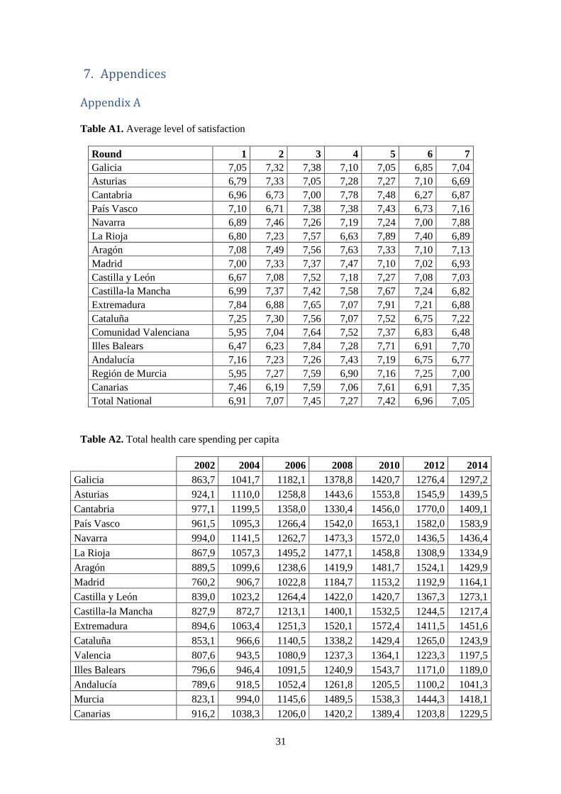
Appendix A
Table A1. Average level of satisfaction
Round 1 2 3 4 5 6 7
Galicia 7,05 7,32 7,38 7,10 7,05 6,85 7,04
Asturias 6,79 7,33 7,05 7,28 7,27 7,10 6,69
Cantabria 6,96 6,73 7,00 7,78 7,48 6,27 6,87
País Vasco 7,10 6,71 7,38 7,38 7,43 6,73 7,16
Navarra 6,89 7,46 7,26 7,19 7,24 7,00 7,88
La Rioja 6,80 7,23 7,57 6,63 7,89 7,40 6,89
Aragón 7,08 7,49 7,56 7,63 7,33 7,10 7,13
Madrid 7,00 7,33 7,37 7,47 7,10 7,02 6,93
Castilla y León 6,67 7,08 7,52 7,18 7,27 7,08 7,03
Castilla-la Mancha 6,99 7,37 7,42 7,58 7,67 7,24 6,82
Extremadura 7,84 6,88 7,65 7,07 7,91 7,21 6,88
Cataluña 7,25 7,30 7,56 7,07 7,52 6,75 7,22
Comunidad Valenciana 5,95 7,04 7,64 7,52 7,37 6,83 6,48
Illes Balears 6,47 6,23 7,84 7,28 7,71 6,91 7,70
Andalucía 7,16 7,23 7,26 7,43 7,19 6,75 6,77
Región de Murcia 5,95 7,27 7,59 6,90 7,16 7,25 7,00
Canarias 7,46 6,19 7,59 7,06 7,61 6,91 7,35
Total National 6,91 7,07 7,45 7,27 7,42 6,96 7,05
Table A2. Total health care spending per capita
2002 2004 2006 2008 2010 2012 2014
Galicia 863,7 1041,7 1182,1 1378,8 1420,7 1276,4 1297,2
Asturias 924,1 1110,0 1258,8 1443,6 1553,8 1545,9 1439,5
Cantabria 977,1 1199,5 1358,0 1330,4 1456,0 1770,0 1409,1
País Vasco 961,5 1095,3 1266,4 1542,0 1653,1 1582,0 1583,9
Navarra 994,0 1141,5 1262,7 1473,3 1572,0 1436,5 1436,4
La Rioja 867,9 1057,3 1495,2 1477,1 1458,8 1308,9 1334,9
Aragón 889,5 1099,6 1238,6 1419,9 1481,7 1524,1 1429,9
Madrid 760,2 906,7 1022,8 1184,7 1153,2 1192,9 1164,1
Castilla y León 839,0 1023,2 1264,4 1422,0 1420,7 1367,3 1273,1
Castilla-la Mancha 827,9 872,7 1213,1 1400,1 1532,5 1244,5 1217,4
Extremadura 894,6 1063,4 1251,3 1520,1 1572,4 1411,5 1451,6
Cataluña 853,1 966,6 1140,5 1338,2 1429,4 1265,0 1243,9
Valencia 807,6 943,5 1080,9 1237,3 1364,1 1223,3 1197,5
Illes Balears 796,6 946,4 1091,5 1240,9 1543,7 1171,0 1189,0
Andalucía 789,6 918,5 1052,4 1261,8 1205,5 1100,2 1041,3
Murcia 823,1 994,0 1145,6 1489,5 1538,3 1444,3 1418,1
Canarias 916,2 1038,3 1206,0 1420,2 1389,4 1203,8 1229,5

32
Picture A3. Questions regading happiness and life satisfaction of the questionnary in the 7th
round (2014) asked in Spain.
33
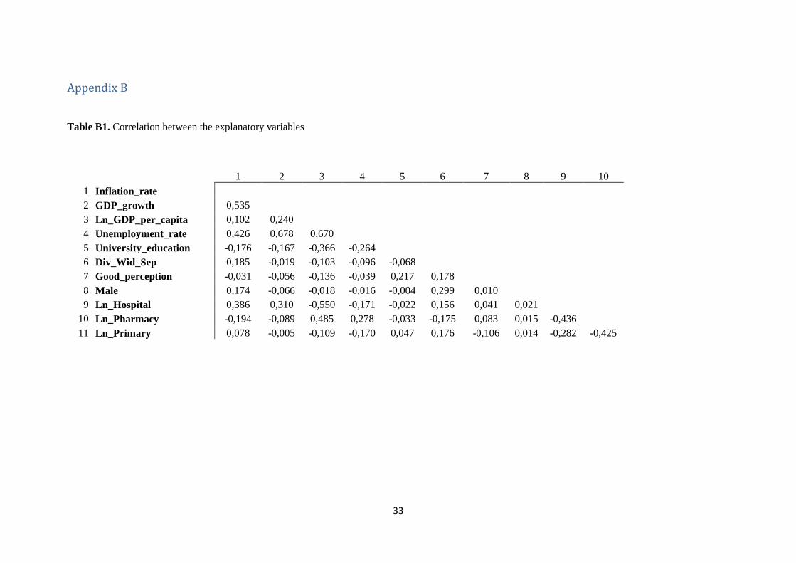
Appendix B
Table B1. Correlation between the explanatory variables
1 2 3 4 5 6 7 8 9 10
1 Inflation_rate
2 GDP_growth 0,535
3 Ln_GDP_per_capita 0,102 0,240
4 Unemployment_rate 0,426 0,678 0,670
5 University_education -0,176 -0,167 -0,366 -0,264
6 Div_Wid_Sep 0,185 -0,019 -0,103 -0,096 -0,068
7 Good_perception -0,031 -0,056 -0,136 -0,039 0,217 0,178
8 Male 0,174 -0,066 -0,018 -0,016 -0,004 0,299 0,010
9 Ln_Hospital 0,386 0,310 -0,550 -0,171 -0,022 0,156 0,041 0,021
10 Ln_Pharmacy -0,194 -0,089 0,485 0,278 -0,033 -0,175 0,083 0,015 -0,436
11 Ln_Primary 0,078 -0,005 -0,109 -0,170 0,047 0,176 -0,106 0,014 -0,282 -0,425
34
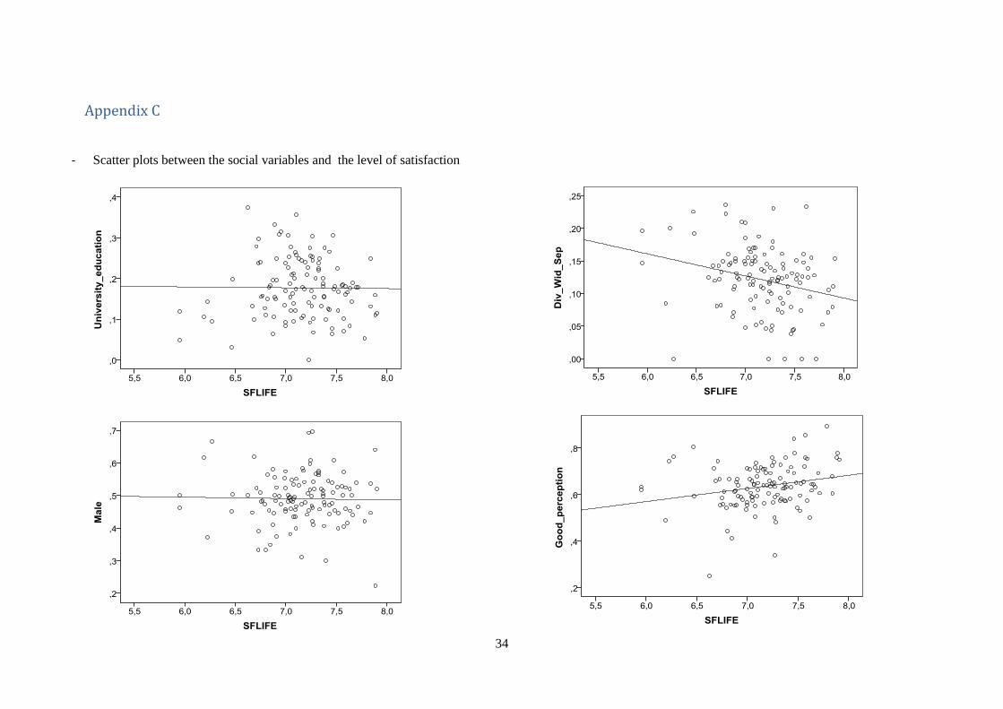
Appendix C
- Scatter plots between the social variables and the level of satisfaction
35
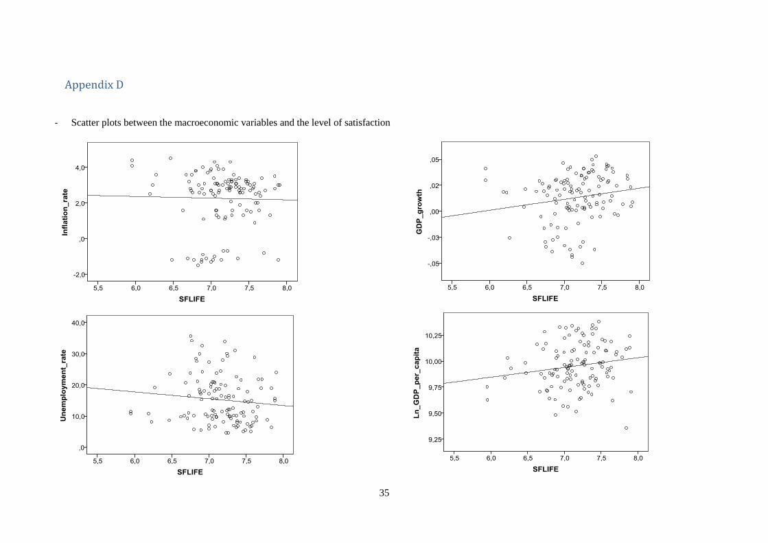
Appendix D
- Scatter plots between the macroeconomic variables and the level of satisfaction