HDPE WOOD-PLASTIC COMPOSITE

MATERIAL MODEL SUBJECT TO DAMAGE

By

GUIBIN LU

A thesis submitted in partial fulfillment of the requirement for the degree of

MASTER OF SCIENCE IN CIVIL ENGINEERING

WASHINGTON STATE UNIVERSITY Department of Civil & Environmental Engineering

May 2002

ii

To the Faculty of Washington State University:

The members of the Committee appointed to examine the thesis of GUIBIN LU find it

satisfactory and recommend that it be accepted.

Chair

iii

ACKNOWLEDGEMENT

This research project was performed at the Department of Civil and Environmental

Engineering at Washington State University, Pullman, Washington. The U.S. Office of Naval

Research provided funding for this research.

A number of professors have helped directly in the preparation of the research thesis.

I would like first to express my appreciation to Dr. William F. Cofer for his advice and

patience while serving as my research committee chair. His thoughts on material modeling are

invaluable for my study and research. The author would also like to thank Dr. John Hermanson

and Dr. Balasingam Muhunthan for their advice and contributions to the research work. Dr.

Hermanson provided the specimen testing data that is crucial for the material model because the

constants obtained from tests were used for ABAQUS computer program. I learned fundamental

knowledge of material modeling from Dr. Muhunthan 's Numerical Modeling of Geomaterials

class.

The author would also like to thank Ying Du, master student Ala’ Abbas and some other

graduate students for their support and friendship during my academic career. Ying Du, Ala’

Abbas helped me to get familiar with the ABAQUS software. We often discuss the problems

related to our research. I would also like to thank graduate students Kevin Jerome Haiar and

Scott Alan Lockyear for their preparing the reference information.

Finally, the author is especially grateful to his parents, and his sisters for their continued

love and encouragement throughout my academic career and for the guidance they have given

me in all aspects of life.

iv

HDPE WOOD-PLASTIC COMPOSITE

MATERIAL MODEL SUBJECT TO DAMAGE

ABSTRACT

By Guibin Lu, M.S. Washington State University

May 2002

Chair: William F. Cofer

The information presented in this thesis is part of an ongoing research project being

performed at Washington State University to develop wood-plastic composite materials for

waterfront structures. Material development has been finished and relevant information can be

found in reference papers. Current research efforts are focused on the development of material

modeling using finite element software. A two-dimensional constitutive model capable of

anisotropic nonlinearity was developed to describe the hyperbolic-tangent behavior of high-

density polyethylene (HDPE) composites. The main objective of this thesis is focused on the

application of an approach for the spectral decomposition of the elasticity tensor to include the

effect of anisotropic behavior and the use of damage concepts to model nonlinearity and failure.

A homogenized continuum based on the effective stress concept was adopted for the theory of

anisotropic damage and elasticity. Damage variables were introduced to describe both the

evolution of the tangent stiffness and the subsequent degradation and failure of the material.

Material softening was assumed to occur when the strain-state for any one of the modes from the

spectral decomposition reaches a critical value. Material constants for tension and compression

were obtained from uniaxial tests. Shear stiffness was obtained from a torsion test and shear

damage parameters were obtained by coupling the x-direction and y-direction constants.

v

A user-defined material subroutine based on the material model was implemented in the

Finite Element software ABAQUS to analyze and predict the behavior of the HDPE material.

Based on the comparisons between the test results and predicted results from ABAQUS for

simple uniaxial models, assumptions regarding the level of orthotropy of the material were

adjusted. In order to evaluate the ability of the material model to accurately simulate behavior

when subjected to biaxial conditions, Iosipescu and five-point bending tests were analyzed.

Although displacement and strength values varied somewhat with those obtained experimentally,

the mode of failure was accurately determined. With further research, the use of the concept of

spectral decomposition and damage holds promise for use in general analysis of members

composed of the HDPE composite material.

vi

TABLE OF CONTENTS

Page

ACKNOWLEDGEMENT iii

ABSTRACT iv

LIST OF TABLES ix

LIST OF FIGURES x

CHAPTER 1

INTRODUCTION

1.1 Background and Overview 1

1.2 The Properties and Mechanical Behavior of the HDPE Material 3

1.3 Objectives 6

CHAPTER 2

LITERATURE REVIEW

2.1 Continuum Damage Mechanics 8

2.2 Effective Stress Concept 9

2.3 Eigentensors in Anisotropic Elasticity 11

2.4 Brief Review of Past Anisotropic Material Failure Criteria 12

CHAPTER 3

CONSTITUTIVE RELATIONSHIP

3.1 Derivation of Constitutive Relation for the HDPE material model (2D) 15

3.2 Summary 22

vii

CHAPTER 4

CHARACTERIZATION OF DAMAGE

4.1 Definition of Damage Variable 23

4.2 Summary 28

CHAPTER 5 UNIAXIAL RESULTS AND DISCUSSION

5.1 Damage Evolution 29

5.2 The Evolution of the Constitutive Matrix 32

5.3 Uniaxial Behavior Modeling 34

5.4 Shear Behavior Modeling 40

5.5 Summary 43

CHAPTER 6 BIAXIAL RESULTS AND DISCUSSION

6.1 Iosipescu test 44

6.2 Five-point beam shear bending test 54

6.3 Summary 63

CHAPTER 7

CONCLUSION 64 APPENDIX

A. Analysis Models and Numerical Data 67 B. ABAQUS User Subroutine For the HDPE Material Model 73

C. ABAQUS Input and Output File for the HDPE Material Model 84

viii

REFERENCES 88

ix

LIST OF TABLES

Page Table 1-1: Tensile and compressive strains and hyperbolic tangent

coefficients, parallel to extrusion 5

Table 1-2: Tensile and compressive strains and hyperbolic tangent coefficients, perpendicular to extrusion 5

Table 1-3: Torsion test results 6 Table 5-1:The damage strain related to eigenmodes 37 Table 5-2:Test data with uniaxial loading perpendicular to grain 37

Table 5-3: Comparison of the results for the material model with uniaxial tests 40 Table 5-4: Comparison of the max shear stress for the HDPE material model and torsion tests 42 Table 6-1: Comparison of the maximum strength for the material model 54 with Iosipescu tests Table 6-2: Comparison of the maximum strength and deflection for the material model

with the five-point bending shear tests 57

x

LIST OF FIGURES

Page

Figure 1-1: Extruded wood/plastic hollow section 3

Figure 1-2: Torsion specimen 3

Figure 1-3: Typical stress-strain relation of the HDPE material 5

Figure 3-1: The derivation of the constitutive matrix of the HDPE material model 21 Figure 4-1: The tensor decomposition of the plane stress tensor 25 Figure 4-2: The derivation of the damage variable 28 Figure 5-1: Damage evolution of the HDPE material model with uniaxial tension loading parallel to extrusion 30 Figure 5-2: Damage evolution of the HDPE material model with uniaxial compression loading parallel to extrusion 30 Figure 5-3: The damage and strain relation of the HDPE material model with uniaxial tension perpendicular to extrusion 31 Figure 5-4: The damage and strain relation of the HDPE material model with uniaxial compression perpendicular to extrusion 31 Figure 5-5: Damage evolution of pure shear case of the HDPE material model 32 Figure 5-6: The stress and strain relation of the HDPE material model with uniaxial tension parallel to extrusion. 38 Figure 5-7: The stress and strain relation of the HDPE material model

with uniaxial compression parallel to extrusion. 38

Figure 5-8: The stress and strain relation of the HDPE material mode with uniaxial tension perpendicular to extrusion. 39 Figure 5-9: The stress and strain relation of the HDPE material model

with uniaxial compression perpendicular to extrusion. 39 Figure 5-10: The single-element HDPE material model used for modeling torsion tests 41

xi

Figure 5-11: Comparison of the pure shear results of the HDPE material model

and torsion test 41 Figure 6-1: Iosipescu shear test setup 45 Figure 6-2: The Iosipescu shear test model within ABAQUS 45 Figure 6-3: Comparison of the load-deflection relation for the Iosipescu test

and the HDPE material model 47 Figure 6-4: Softening damage parameter for mode 1 with orthotropic damage properties 48 Figure 6-5: Softening damage parameter for mode 2 with orthotropic damage properties 48 Figure 6-6: Softening damage parameter for shear with orthotropic damage properties 49 Figure 6-7: Softening damage parameter for mode 1 with isotropic damage properties 49 Figure 6-8: Softening damage parameter for mode 2 with isotropic damage properties 50 Figure 6-9: Softening damage parameter for shear with isotropic damage properties 50 Figure 6-10: Principal strain at maximum strength with orthotropic damage properties 52 Figure 6-11: Principal strain at failure with orthotropic damage properties 52 Figure 6-12: Principal strain prior to failure with isotropic damage properties 53 Figure 6-13: Principal strain at maximum strength with isotropic damage properties 53 Figure 6-14: Principal strain at failure with isotropic damage properties 54

Figure 6-15: Photograph of the five-point bending shear test setup 55

Figure 6-16: Five-point bending shear test setup 55

Figure 6-17: Five-point bending shear test model within ABAQUS 56

xii

Figure 6-18: Comparison of the load-deflection relation for the five-point bending test and the HDPE material model 57

Figure 6-19: Softening damage parameter for mode 2 with orthotropic damage properties 58 Figure 6-20: Softening damage parameter for shear with orthotropic damage properties 59 Figure 6-21: Softening damage parameter for mode 1 with isotropic damage properties 59 Figure 6-22: Softening damage parameter for mode 2 with isotropic damage properties 60 Figure 6-23: Softening damage parameter for shear with isotropic damage properties 60 Figure 6-24: The shear failure displayed in 5-point specimen test 61 Figure 6-25: Shear strain at maximum strength with orthotropic damage properties 62 Figure 6-26: Shear strain at maximum strength with isotropic damage properties 62

1

CHAPTER 1

Introduction

1.1 Background and Overview

Historically, preservative-treated wood timber has been utilized for structural elements

within marine fender systems. However, as waterways have become less polluted, the traditional

wood members are subjected to increasing degradation generated by marine borers. Furthermore,

public concerns about water pollution in harbors have resulted in restrictions on the use of wood

preservatives. As a result, an alternative material to replace the traditional wood material is

required. The U.S. Office of Naval Research funded this research project with the Department of

Civil and Environmental Engineering, Washington State University to investigate the feasibility

of using a wood-plastic composite material (WPC) as an alternative for components of fender

systems. Wood-plastic composite materials (WPC) have several benefits compared to the

traditional wood material. First, it is resistant to insects, marine borers and rot when used for

structural members. Without the preservative treatments, there is no environmental impact. Also,

reduced production costs make wood-plastic economical for many structural applications.

The information presented in this thesis is related to two parts of the research project.

One is High Density Polyethylene (HDPE) material development and the other is the use of

Finite Element analysis software ABAQUS to model the nonlinear behavior of the HDPE

material. The experimental testing was performed on extruded wood-based composite material,

which was approximately composed of 70% wood and 30% high-density polyethylene (HDPE)

2

(Cofer et al., 1998). The properties of a number of wood-based composite materials have been

obtained through the compression and tensile testing of specimens. Uniaxial testing has shown

that wood/plastic composites display a nonlinear constitutive behavior in hyperbolic tangent

form.

A simple plane stress material model for uniaxial applications was developed (Cofer,

1998, 1999), for which non-linearity from finite deformations and material behavior was

included. However, that model cannot be directly applied to more general two-dimensional

applications. In this thesis, a new material model is presented to describe the nonlinear behavior

shown in experimental tests for plane stress applications, which is based on Continuum Damage

Mechanics (CDM) and the spectral decomposition of the constitutive tensor.

1.2 The Properties and Mechanical Behavior of the HDPE Material

In this project, the high-density polyethylene (HDPE) composite material was chosen to

be modeled. Specifically, the HDPE composite was composed of 58% maple flour (American

Wood Fiber #4010), 31% HDPE (equistar LB0100 00), 8% inorganic filler, and 3% processing

aids. For specimen tests, the HDPE material was extruded using a conical twin-screw extruder

(Cincinnati-Milicron CM80) and a stranding die (Lockyear, 1999).

Tensile, compression, bending and torsion tests were performed on small HDPE

composite specimens to determine its properties. Interested readers can find detailed information

on experimental methods from the reports of Haiar (2000) and Lockyear (1999). Here, examples

3

of testing specimens are given.

Figure 1-1 shows typical extruded wood/plastic hollow test sections, which were used in

uniaxial and five-point bending tests.

Figure 1-1: Extruded wood/plastic hollow section (Lockyear, 1999)

Figure 1-2 shows the torsion specimen. The shear modulus used as input for the HDPE

model was obtained from torsion tests.

Figure 1-2: Torsion specimen (Lockyear, 1999)

4

Through the compression and tension tests of small specimens, the properties of the

HDPE composite material have been obtained. In each case, it was found that the uniaxial stress-

strain relationships are similar in shape, no matter how loads were applied. Such relationships

can be represented by a hyperbolic-tangent function (Cofer, 1999):

)tanh( εσ ba= , (1.1)

and

)(cosh2 εε

σb

ab=

∂∂ . (1.2)

Also, when 0=ε ,

MOEab ==∂∂εσ (Modulus of Elasticity) (1.3)

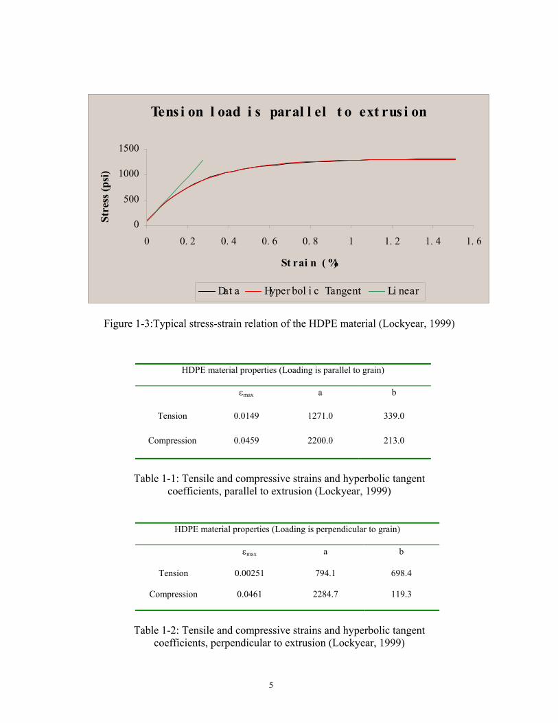
Here, σ and ε are uniaxial stress and strain, respectively, and a and b are constants. A typical

stress-strain relationship of the HDPE material is shown in Figure 1-3, which was obtained when

the load was applied in tension parallel to the material grain.

From the physical specimen tests, it was found that the HDPE composite material

behaves differently in tension cases versus compression cases with respect to different values of

stiffness and strength. One of the differences is the maximum strain, which is defined by the

onset of softening or fracture. Table 1-1 and Table 1-2 show the tensile and compressive

maximum strain values and hyperbolic tangent constitutive parameters. Another interesting

phenomenon observed is that the HDPE composites are quite flexible in shear, with a shear

modulus obtained from torsion tests. Table 1-3 shows the maximum strain and strength values

obtained from torsion tests.

5

Tens i on l oad i s paral l el t o ext rus i on

0

500

1000

1500

0 0. 2 0. 4 0. 6 0. 8 1 1. 2 1. 4 1. 6

St rai n ( %)

Stre

ss (p

si)

Dat a Hyper bol i c Tangent Li near

Figure 1-3:Typical stress-strain relation of the HDPE material (Lockyear, 1999)

HDPE material properties (Loading is parallel to grain)

εmax a b

Tension 0.0149 1271.0 339.0

Compression 0.0459 2200.0 213.0

Table 1-1: Tensile and compressive strains and hyperbolic tangent

coefficients, parallel to extrusion (Lockyear, 1999)

HDPE material properties (Loading is perpendicular to grain)

εmax a b

Tension 0.00251 794.1 698.4

Compression 0.0461 2284.7 119.3

Table 1-2: Tensile and compressive strains and hyperbolic tangent

coefficients, perpendicular to extrusion (Lockyear, 1999)

6

HDPE material properties (From torsion tests)

εmax Maximum Strength (psi) Shear Modulus (psi)

Average Value 0.022 1006.3 132077.7

Table 1-3: Torsion test results (Lockyear, 1999)

1.3 Objectives

The purpose of the work of this thesis is to provide a new wood composite material

model, based on concepts of damage, to extend the nonlinear behavior observed in uniaxial

physical testing on the HDPE material to two-dimensional analysis. At the same time, it is

necessary to evaluate the behavior related to anisotropy through the application of spectral

decomposition of the constitutive tensor. Specifically, the objectives are:

1. Develop the theory of the material model.

2. Implement the model in Finite Element software and calibrate with uniaxial test data.

3. Validate its ability to accurately model biaxial behavior by modeling biaxial tests.

To realize these objectives, equivalent constitutive relations were determined, and

formulations for damage evolution were developed based on Continuum Damage Mechanics and

the effective stress concept. Also, some constitutive assumptions were made for this material

model:

1. The HDPE material model is appropriate for plane stress conditions.

7

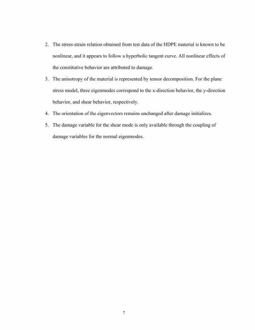
2. The stress-strain relation obtained from test data of the HDPE material is known to be

nonlinear, and it appears to follow a hyperbolic tangent curve. All nonlinear effects of

the constitutive behavior are attributed to damage.

3. The anisotropy of the material is represented by tensor decomposition. For the plane

stress model, three eigenmodes correspond to the x-direction behavior, the y-direction

behavior, and shear behavior, respectively.

4. The orientation of the eigenvectors remains unchanged after damage initializes.

5. The damage variable for the shear mode is only available through the coupling of

damage variables for the normal eigenmodes.

8

CHAPTER 2

Literature Review

The behavior of the HDPE wood composite material is influenced by its nonlinearity and

its anisotropy. The background to both is presented in this chapter.

2.1 Continuum Damage Mechanics

The analysis for the HDPE composite material subject to damage is based upon the

behavior at the microscopic scale, as predicted using the concepts of effective constitutive and

evolution equations (Caiazzo and Costanzo, 1999).

As Caiazzo and Costanzo indicated, “effective constitutive equations describe the

behavior of a single material element of an equivalent homogeneous medium.” The effective

constitutive equations will vary nonlinearly during the process of loading. These equations are

developed to be valid for any deformation history that a material point will experience. To obtain

equations of this type is the fundamental goal of any theory of effective properties of composites.

Among these theories, Continuum Damage Mechanics (CDM) and homogenization theory (HT)

are the two most prominent (Caiazzo and Costanzo, 1999). In this material model, the

Continuum Damage Mechanics concept was used.

Caiazzo and Costanzo defined Continuum Damage Mechanics (CDM) as “a

phenomenological approach where the mathematical description of a certain type of microscopic

damage mechanism is given in terms of some appropriately defined damage variables”. After

those variables have been determined, the constitutive relation can be obtained using continuum

9

thermodynamic theories of constitutive equations (Coleman and Gurtin, 1967; Coleman and

Noll, 1963; Germain et al., 1983). The constitutive relation obtained will correspond to a new

damage state. As the damage variables change and the properties of the nonlinearity develop, the

constitutive relation will change accordingly because it is a function of those variables.

2.2 Effective Stress Concept

To develop a damage theory, the first thing is to define a damage variable because

damage is not a quantity that can be measured. The theory of Continuum Damage Mechanics

provides several ways to provide an equivalent homogeneous medium to describe damage, one

of which is the use of the effective stress concept. Lemaitre (1983) gave a clear definition for

effective stress: “ A damaged volume of material under the applied stress σ shows the same

strain response as the undamaged one submitted to the effective stress σ~ .” In an energy sense,

this definition can be explained as the energy stored in the damaged material is equivalent to the

energy in a fictious undamaged material.

The damage variable can be measured through the overall section area of a material

element, S , and the effective area after damage occurred, S~ .

S

SSD~

−= . (2.1)

Different values of the damage variable correspond to different states of the material

element.

0=D corresponds to the undamaged state;

1=D corresponds to the fully-damaged state;

10

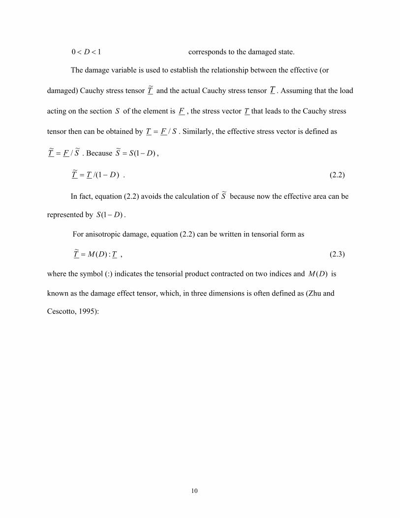
10 << D corresponds to the damaged state.

The damage variable is used to establish the relationship between the effective (or

damaged) Cauchy stress tensor T~ and the actual Cauchy stress tensor T . Assuming that the load

acting on the section S of the element is F , the stress vector T that leads to the Cauchy stress

tensor then can be obtained by SFT /= . Similarly, the effective stress vector is defined as

SFT ~/~ = . Because )1(~ DSS −= ,

)1/(~ DTT −= . (2.2)

In fact, equation (2.2) avoids the calculation of S~ because now the effective area can be

represented by )1( DS − .

For anisotropic damage, equation (2.2) can be written in tensorial form as

TDMT :)(~ = , (2.3)

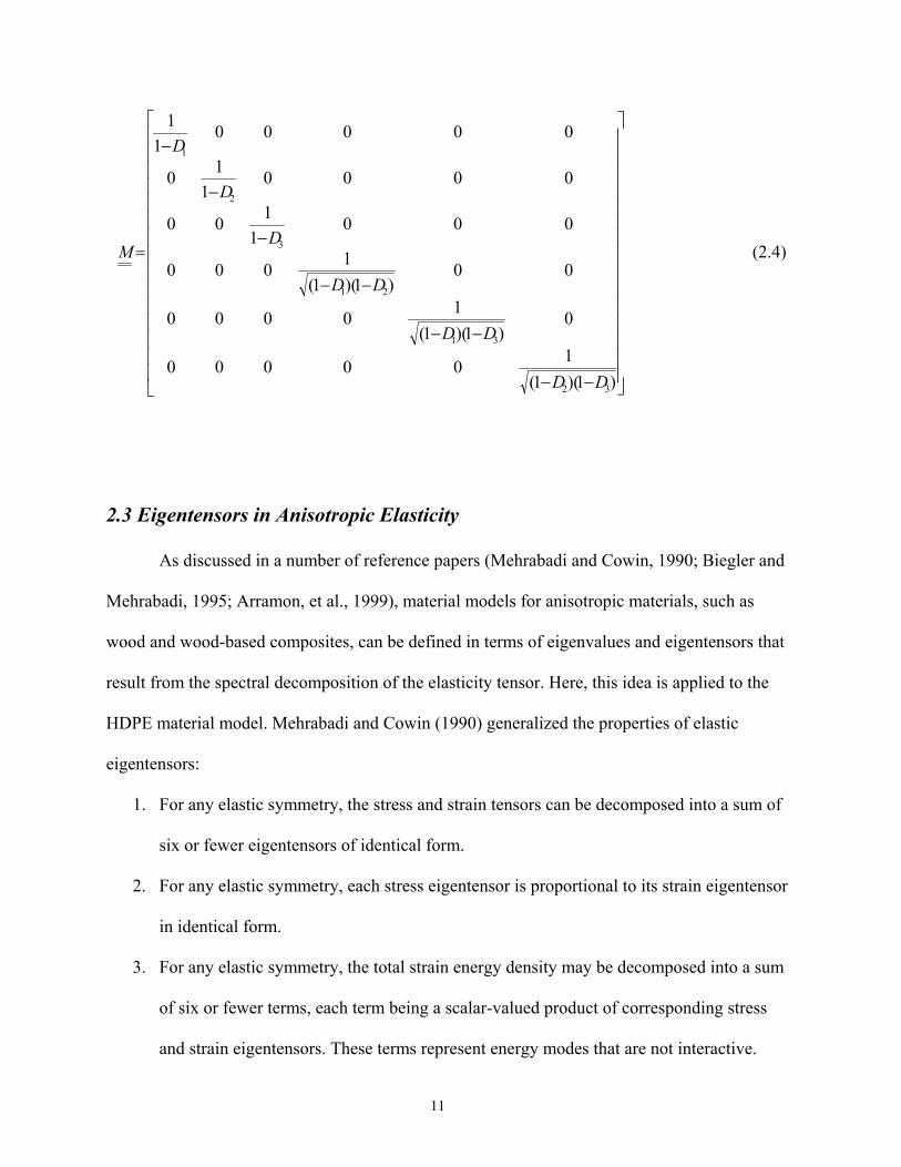
where the symbol (:) indicates the tensorial product contracted on two indices and )(DM is

known as the damage effect tensor, which, in three dimensions is often defined as (Zhu and

Cescotto, 1995):

11

−−

−−

−−

−

−

−

=

)1)(1(100000

0)1)(1(

10000

00)1)(1(

1000

0001

100

00001

10

000001

1

32

31

21

3

2

1

DD

DD

DD

D

D

D

M (2.4)

2.3 Eigentensors in Anisotropic Elasticity

As discussed in a number of reference papers (Mehrabadi and Cowin, 1990; Biegler and

Mehrabadi, 1995; Arramon, et al., 1999), material models for anisotropic materials, such as

wood and wood-based composites, can be defined in terms of eigenvalues and eigentensors that

result from the spectral decomposition of the elasticity tensor. Here, this idea is applied to the

HDPE material model. Mehrabadi and Cowin (1990) generalized the properties of elastic

eigentensors:

1. For any elastic symmetry, the stress and strain tensors can be decomposed into a sum of

six or fewer eigentensors of identical form.

2. For any elastic symmetry, each stress eigentensor is proportional to its strain eigentensor

in identical form.

3. For any elastic symmetry, the total strain energy density may be decomposed into a sum

of six or fewer terms, each term being a scalar-valued product of corresponding stress

and strain eigentensors. These terms represent energy modes that are not interactive.

12

In order to identify the proportional stress and strain eigentensors of an anisotropic solid,

a second rank stiffness tensor, C, was developed by Mehrabadi and Cowin (1990). The stress

tensor is represented by T and the strain tensor is represented by E . The Ath eigenvalue )( AΛ

of C satisfies the equation

0ˆ)()(=Λ−

A

A EIC , (2.5)

where )(ˆ A

E is the A th strain eigentensor and I is the identity tensor.

From the first property stated above, the total strain is the sum of all of the eigenstrains.

Similarly, the total stress can be found by summing the eigenstresses. The second property can

be written for the A th eigenvalue as

)()( ˆˆ A

A

AET Λ= . (2.6)

The third property can be represented by

∑=

=Σn

A

AAET

1

)()( ˆˆ2 , (2.7)

where Σ is the total strain energy density.

Again, it is noted that each of the addends of this sum quantifies an energy mode that is

independent of any other terms. These non-interactive energy modes are used to set up a failure

criterion taking into account anisotropy, as mentioned subsequently.

2.4 Brief Review of Past Anisotropic Material Failure Criteria

This research is developed from ideas presented by Mehrabadi and Cowin (1990),

Biegler and Mehrabadi (1995), Schreyer and Zuo (1995), and Arramon, et al. (2000). The

13

formulation for their failure criteria is based upon the idea of the spectral decomposition of the

elastic tensor into the so-called Kelvin modes. Mehrabadi and Cowin (1990) introduced the idea

and defined Kelvin modes in detail.

According to their theories, the strain energy, U, is decomposed into the sum of modal

energies )( AU . After these energy modes have been defined for a given material, the limit values

are determined from uniaxial tests. Biegler and Mehrabadi (1995) and Schreyer and Zuo (1995)

predict that failure occurs when the energy of each mode reaches a limit value. Those failure

criteria are based on Kelvin modes. Kelvin modes are actually the eigenmodes discussed

previously. However, this method cannot account for the difference in material strength for

tensile and compressive stress. To find a way to include the difference in tensile and compressive

failure modes, Arramon, et al (2000) proposed failure criteria evaluated for positive and negative

maximum eigenstress magnitudes separately.

2)()( )(2 A

TATAU σ=Λ and 2)(

)( )(2 AC

ACAU σ=Λ . (2.8)

Here, )( ATσ are the tensile eigenstress magnitudes that can be determined from tests and )( A

Cσ are

the compressive eigenstress magnitudes that can be determined from tests. AΛ are the

eigenvalues. ATU )( and A

CU )( are the modal energy values for tension and compression. Then the

strength envelope developed from Kelvin modes is in the form:

0))(( )()()()( =−− AC

AAT

A σσσσ (2.9)

Arramon, et al. (2000) also note that, for most materials, additional modes of failure

exist, which are independent of the Kelvin modes. Complementary failure modes were thus

introduced, corresponding to maximum principal stress, which can be written as

14

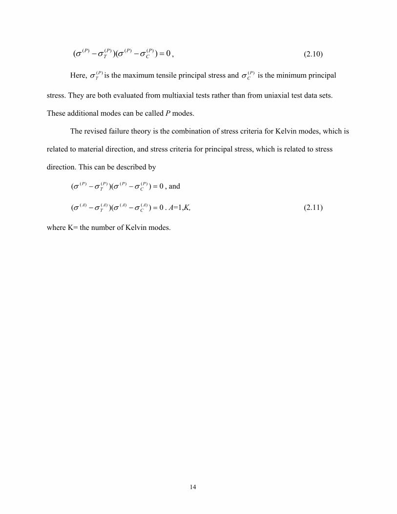
0))(( )()()()( =−− PC

PPT

P σσσσ , (2.10)

Here, )(PTσ is the maximum tensile principal stress and )(P

Cσ is the minimum principal

stress. They are both evaluated from multiaxial tests rather than from uniaxial test data sets.

These additional modes can be called P modes.

The revised failure theory is the combination of stress criteria for Kelvin modes, which is

related to material direction, and stress criteria for principal stress, which is related to stress

direction. This can be described by

0))(( )()()()( =−− PC

PPT

P σσσσ , and

0))(( )()()()( =−− AC

AAT

A σσσσ . A=1,K, (2.11)

where K= the number of Kelvin modes.

15

CHAPTER 3

Constitutive Relationship

Within a material model, the constitutive relationship is used to connect the stress domain

with the strain domain. For the material model described here, the nonlinear stress/strain

behavior is modeled through the use of damage, which represents the change in the makeup of

the material. The nonlinearity and, hence, damage is assumed to initiate and evolve from the

initial loading. The concept of damage is taken from the theory of Continuum Damage

Mechanics, in which effective (or equivalent) stress is used to account for its effect. In this

chapter, the development of the constitutive matrix within the material model is presented.

3.1 Derivation of the Constitutive relation for the HDPE Material Model (Two-dimensional)

Without the influence of damage, the constitutive law between stresses and strains is

linear. This new material model is for two dimensional plane stress applications. Therefore, for

two dimensional plane stress cases, the linear elastic constitutive relation between stresses and

strains for orthotropic materials is well known as:

εσ ⋅= C (3.1)

and

−−

=

121221

2221

1211

1221 )1(0000

11

GE

EC

υυυ

υ

υυ . (3.2)

16

Like other anisotropic materials, the HDPE material behaves differently in tension,

compression and shear. So this material model is assumed to be orthotropic and the initial values

of 11E and 22E are obtained by averaging the tensile and compressive test data. Then 12v and 21v

are assumed. In a more general case, all the coefficients of equation (3.2) could be obtained from

tests.

To describe the anisotropic behavior of the HDPE material, the idea of tensor

decomposition is used (Biegler and Mehrabadi, 1993 and 1995). For the two-dimensional plane

stress case, the total stress σ and the total strain ε are decomposed into three eigentensors,

which correspond to three eigenvalues accordingly. The strain eigentensor )(ˆ A

E and the

eigenvalues AΛ of C satisfy equation (2.6), as described in Chapter 2.3.

To obtain stress eigentensors and strain eigentensors, the eigenvalue equation must be

solved. For convenience, C is denoted as:

=

66

2221

1211

20000

CCCCC

C . (3.3)

Then, the equation can be rewritten as:

=

Λ−Λ−

Λ−

000

220000

12

22

11

66

2221

1211

EEE

CCC

CC . (3.4)

Mathematically, the characteristic equation is:

[ ] 0))(()2( 2112221166 =−Λ−Λ−Λ− CCCCC . (3.5)

From this equation, the roots may be obtained:

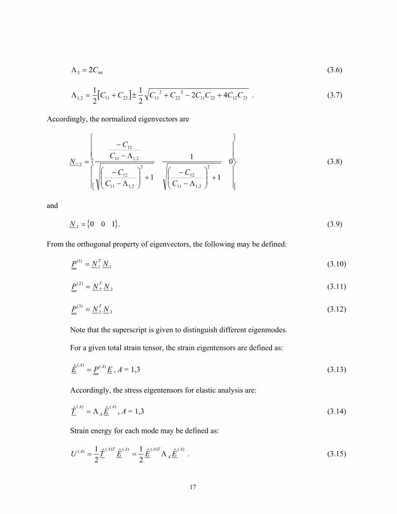
17

663 2C=Λ (3.6)

[ ] 211222112

222

1122112,1 4221

21 CCCCCCCC +−+±+=Λ . (3.7)

Accordingly, the normalized eigenvectors are

+

Λ−−

+

Λ−−

Λ−−

= 0

1

1

12

2,111

12

2

2,111

12

2,111

12

2,1

CC

CC

CC

N (3.8)

and

{ }1003 =N . (3.9)

From the orthogonal property of eigenvectors, the following may be defined:

11)1( NNP T= (3.10)

22)2( NNP T= (3.11)

33)3( NNP T= (3.12)

Note that the superscript is given to distinguish different eigenmodes.

For a given total strain tensor, the strain eigentensors are defined as:

EPE AA )()(ˆ = , A = 1,3 (3.13) Accordingly, the stress eigentensors for elastic analysis are:

)()( ˆˆ A

A

AET Λ= , A = 1,3 (3.14)

Strain energy for each mode may be defined as:

)()()()()( ˆˆ

21ˆˆ

21 A

A

TAATAA EEETU Λ== . (3.15)

18

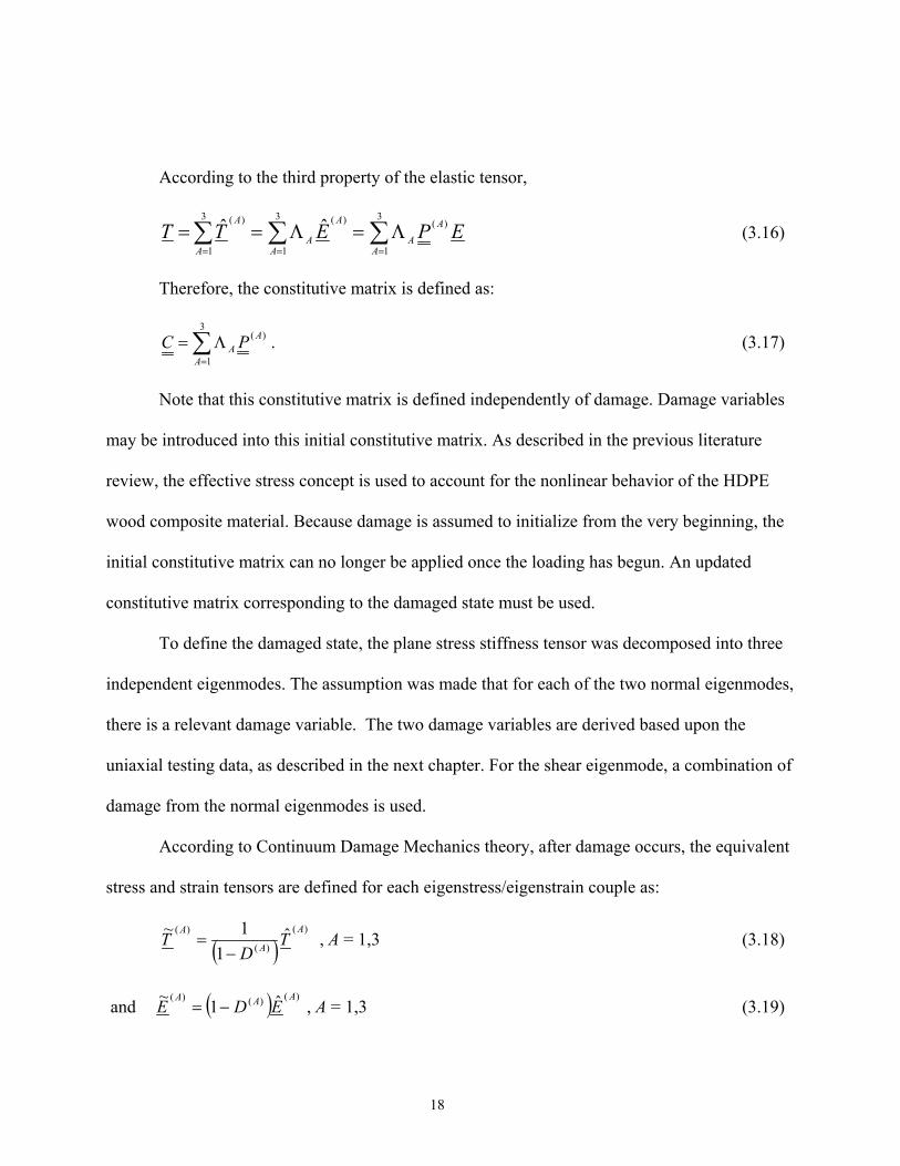
According to the third property of the elastic tensor,

∑∑∑===

Λ=Λ==3

1

)(3

1

)(3

1

)( ˆ ˆ

A

AA

A

A

AA

AEPETT (3.16)

Therefore, the constitutive matrix is defined as:

∑=

Λ=3

1

)(

A

AA PC . (3.17)

Note that this constitutive matrix is defined independently of damage. Damage variables

may be introduced into this initial constitutive matrix. As described in the previous literature

review, the effective stress concept is used to account for the nonlinear behavior of the HDPE

wood composite material. Because damage is assumed to initialize from the very beginning, the

initial constitutive matrix can no longer be applied once the loading has begun. An updated

constitutive matrix corresponding to the damaged state must be used.

To define the damaged state, the plane stress stiffness tensor was decomposed into three

independent eigenmodes. The assumption was made that for each of the two normal eigenmodes,

there is a relevant damage variable. The two damage variables are derived based upon the

uniaxial testing data, as described in the next chapter. For the shear eigenmode, a combination of

damage from the normal eigenmodes is used.

According to Continuum Damage Mechanics theory, after damage occurs, the equivalent

stress and strain tensors are defined for each eigenstress/eigenstrain couple as:

( ))(

)(

)( ˆ1

1~ A

A

AT

DT

−= , A = 1,3 (3.18)

and ( ) )()()( ˆ1~ AAAEDE −= , A = 1,3 (3.19)

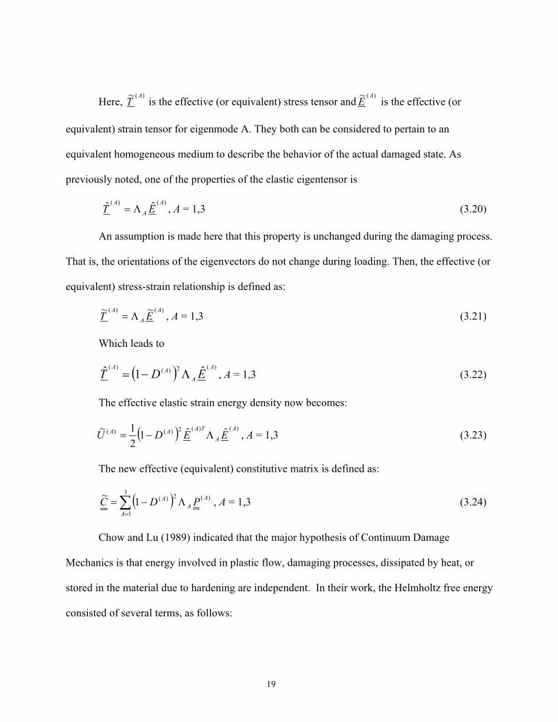
19

Here, )(~ A

T is the effective (or equivalent) stress tensor and)(~ A

E is the effective (or

equivalent) strain tensor for eigenmode A. They both can be considered to pertain to an

equivalent homogeneous medium to describe the behavior of the actual damaged state. As

previously noted, one of the properties of the elastic eigentensor is

)()( ˆˆ A

A

AET Λ= , A = 1,3 (3.20)

An assumption is made here that this property is unchanged during the damaging process.

That is, the orientations of the eigenvectors do not change during loading. Then, the effective (or

equivalent) stress-strain relationship is defined as:

)()( ~~ A

AA

ET Λ= , A = 1,3 (3.21)

Which leads to

( ) )(2)()( ˆ1ˆ A

AAA

EDT Λ−= , A = 1,3 (3.22)

The effective elastic strain energy density now becomes:

( ) )()(2)()( ˆˆ121~ A

A

TAAA EEDU Λ−= , A = 1,3 (3.23)

The new effective (equivalent) constitutive matrix is defined as:

( )∑=

Λ−=3

1

)(2)(1~A

AA

A PDC , A = 1,3 (3.24)

Chow and Lu (1989) indicated that the major hypothesis of Continuum Damage

Mechanics is that energy involved in plastic flow, damaging processes, dissipated by heat, or

stored in the material due to hardening are independent. In their work, the Helmholtz free energy

consisted of several terms, as follows:

20

[ ])()()()( ~1 Ad

Ap

Ae

A U ψψρ

ψ ++= (3.25)

where )(~ AeU is the elastic strain energy, )( A

pψ is the free energy due to plastic hardening, and )( Adψ

is the free energy due to damage hardening. Within this material model, only elastic/damage

behavior was considered.

In summary, the whole process discussed above is generalized as a flow chart, which is

shown in Figure 3-1 (see next page):

21

Figure 3-1: The derivation of the constitutive matrix

of the HDPE material model

Three eigenmodes

Eigenmode 1: Λ1, 1N , 1P , 1T , 1E

Eigenmode 2: Λ2, 2N , 2P , 2T , 2E

Eigenmode 3: Λ3, 3N , 3P , 3T , 3E

The second rank stiffness tensor

C

After Tensor Decomposition

The second rank stiffness tensor

∑=

Λ=3

1

)(

A

AA PC

After Damage Occurs

The Effective Stress )()( ~~ A

AA

ET Λ=

The updated stiffness tensor

( )∑=

Λ−=3

1

)(2)(1~A

AA

A PDC

The Third Property of

The Elastic Tensor

The Effective Stress

( ))(

)(

)( ˆ1

1~ A

A

AT

DT

−=

)()( ˆˆ A

A

AET Λ=

22

3.2 Summary:

In this chapter, the concept and background of Continuum Damage Mechanics were

introduced. The effective stress concept, acting as a bridge between the undamaged state and

damaged state, provides a way to describe the influence of damage. The idea of tensor

decomposition was introduced to describe the material anisotropy. Based upon these concepts,

the formulation of a constitutive relation that is valid during the nonlinear process was derived.

Mathematically, the constitutive matrix obtained from the derivation is actually a function of

damage variables, so that the constitutive matrix will change as damage develops.

23

CHAPTER 4

Characterization of Damage

For the two-dimensional model, there are three eigenmodes. The normal eigenmodes

were assumed to relate to the uniaxial behavior of the HDPE material. So, the hyperbolic tangent

function displayed in uniaxial behavior was applied to the two normal eigenmodes. Each

eigenmode has a corresponding damage variable due to the fact that damage is a function of the

magnitude of the eigenstrain. Because the assumption was made previously that damage was the

cause of the nonlinearity and the hyperbolic tangent function obtained from tests shows the trend

of the nonlinearity, damage of the two normal modes can be derived by taking the derivative of

the hyperbolic tangent function. In addition to the normal eigenmodes, there is a shear damage

mode that is the combination of the normal eigenmodes. Within an eigenmode, separate damage

variables were used for tension and for compression. The constitutive matrix is looked upon as a

function of damage variables, and it changes with the evolution of damage.

4.1 Definition of Damage Variables

The formulation of damage evolution is based on the hyperbolic tangent function. As

indicated in the previous chapter, the uniaxial stress-strain relationship for the HDPE material

follows the hyperbolic tangent curve, given in equations (1.1), (1.2) and (1.3).

24

Some assumptions were made for this model in Chapter 1, one of which is that the

nonlinearity of the HDPE material is totally caused by damage. As is well known, the ratio of the

change of stress increment and strain increment is the stiffness, and the change of the stiffness

can be the measure of damage. Therefore, after taking the derivative of equation (1.2), the

damage variable for uniaxial behavior has the following form:

−= ε

aabhD 2sec1 (4.1)

where a and b are obtained from uniaxial tests. See Table 1-1.

From the table, it is observed that the damage variable for tension must be different from

that of compression no matter how the loads are applied.

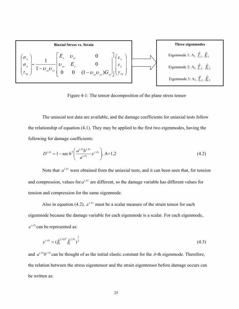
Biaxial mechanical behavior can be thought of as the interaction of x-direction and y-

direction uniaxial behavior. Within this material model, the idea of tensor decomposition

(Biegler and Mehrabadi, 1993 and 1995) was used to describe the anisotropic properties of the

HDPE material. After decomposition, three eigenmodes were obtained for the plane stress case,

and each one corresponds to a specific eigenvalue. The three eigenmodes generated by the

decomposition of a plane stress tensor are easily related to the x-direction uniaxial behavior, y-

direction uniaxial behavior, and shear behavior for this type of directional material. Thus, each

eigenmode describes one type of behavior.

25

Figure 4-1: The tensor decomposition of the plane stress tensor

The uniaxial test data are available, and the damage coefficients for uniaxial tests follow

the relationship of equation (4.1). They may be applied to the first two eigenmodes, having the

following for damage coefficients:

−= )(

)(

)()(2)( sec1 A

A

AAA

abahD ε , A=1,2 (4.2)

Note that )( Aa were obtained from the uniaxial tests, and it can been seen that, for tension

and compression, values for )( Aa are different, so the damage variable has different values for

tension and compression for the same eigenmode.

Also in equation (4.2), )( Aε must be a scalar measure of the strain tensor for each

eigenmode because the damage variable for each eigenmode is a scalar. For each eigenmode,

)( Aε can be represented as:

21

)()()( )ˆˆ(ATAA EE=ε (4.3)

and )()( AA ba can be thought of as the initial elastic constant for the A-th eigenmode. Therefore,

the relation between the stress eigentensor and the strain eigentensor before damage occurs can

be written as:

Biaxial Stress vs. Strain

xy

y

x

τ

σσ

=

−−

xyyxxy

yyx

vyx

yxxy GE

E

)1(0000

11

υυυ

υ

υυ

xy

y

x

γ

εε

Three eigenmodes

Eigenmode 1: Λ1, 1T , 1E

Eigenmode 2: Λ2, 2T , 2E

Eigenmode 3: Λ3, 3T , 3E

26

)()()()( ˆˆ AAAAEbaT = (4.4)

According to Mehrabadi and Cowin (1990), one of the properties of the eigentensors is

that each stress eigentensor is proportional to its strain eigentensor, which is represented by:

)()( ˆˆ A

A

AET Λ= . (4.5)

Therefore, )()( AA ba can be written in the form of the eigenvalue AΛ . Equation (4.2) can

then be rewritten as:

Λ−= )(

)(2)( sec1 A

AAA

ahD ε . A=1,2 (4.6)

Within the material model, there is no independent damage for the shear mode. The

reason is that, in reality, shear failure is a passive failure state. Material failure caused by shear

loading results from cracks in the x-direction and y-direction. Based upon this fact, the damage

variable for the shear mode is obtained by

)1)(1(1 )2()1()( DDD S −−−= . (4.7)

From torsion test specimens, it was also observed that the shear failure plane has a 45-

degree angle with the x-z plane and the y-z plane. However, a problem arises for the pure shear

case. Because strain components on material axes are zero for pure shear, )1(D and )2(D must

remain zero during damage evolution, and )(sD must be zero. But, experimentally, the material

does exhibit damage when subjected to pure shear loading. To have a non-zero shear damage

parameter, shear strain is assumed to contribute equally to the damage evolution of the other two

modes. The reasoning is that, with the assumption of independence of energy between the

various modes, the shear strain was treated as if it acts alone. Then, the principal strains from that

27

pure shear case were assumed to act in tension and compression at a 45-degree angle to the 1-

axis and 2-axis, causing simultaneous evolution of tensile and compressive damage.

As mentioned in Chapter 3, within the material model, only elastic/damage behavior was

considered. If this idea is applied to the stress calculation, then, the equivalent eigenstress

becomes,

( )

Λ−=

∂∂

=)()(

)(

)()( ˆ1ˆ

~ A

AA

A

AA

EDE

T ψρ (4.8)

Then, after damage occurs, for each eigenmode, the new stress-strain relations can be

written as:

( ) )(2)()( ˆ1ˆ A

AAA

EDT Λ−= , A = 1,3 (4.9)

The equivalent eigenstress rate is

( ) ( ) )()()()(2)(

)(

ˆ12ˆ1ˆ A

AAA

A

AA

A

EDDEDT Λ−−Λ−=•

&& (4.10) Incrementally, equation (4.10) can be written as:

( ) ( ) )()()()(2)()( ˆ12ˆ1ˆ A

AAAA

AAA

EDDEDT Λ−∆−∆Λ−=∆ (4.11)

28

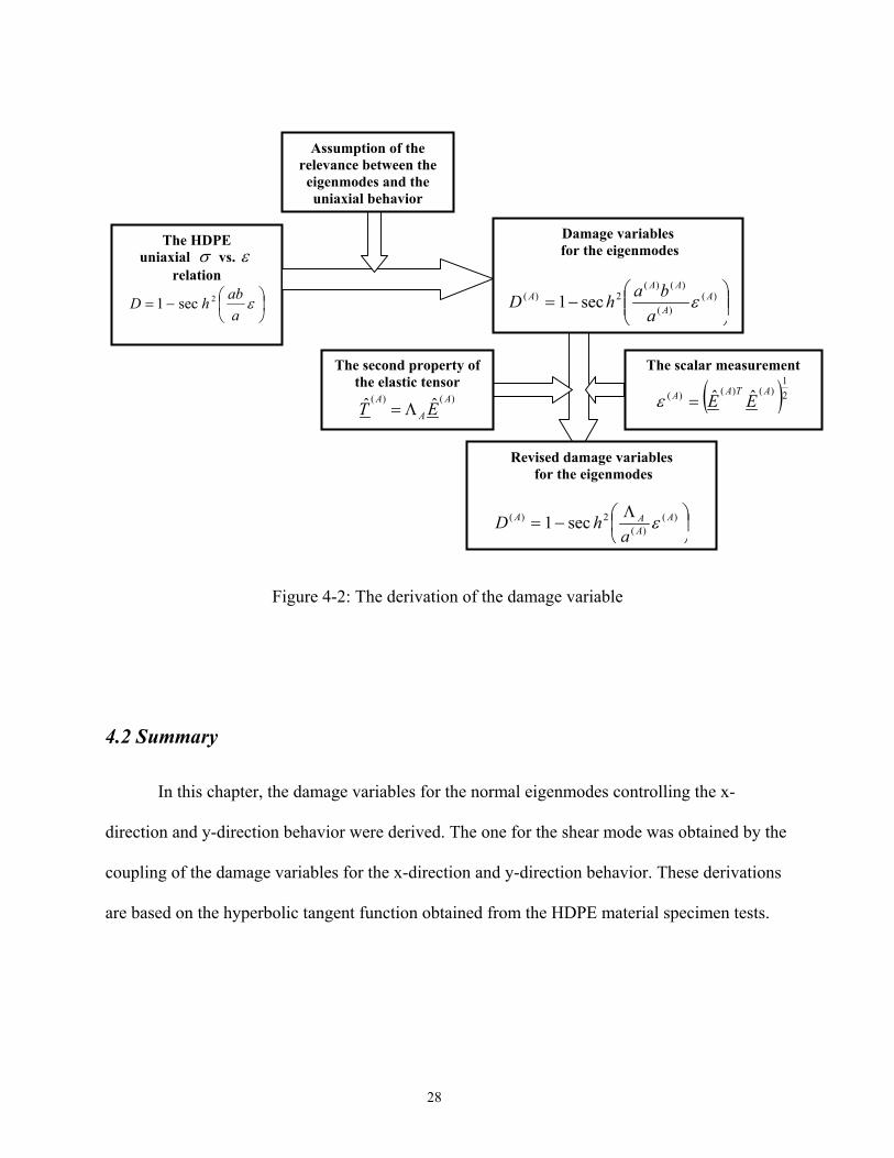
Figure 4-2: The derivation of the damage variable

4.2 Summary

In this chapter, the damage variables for the normal eigenmodes controlling the x-

direction and y-direction behavior were derived. The one for the shear mode was obtained by the

coupling of the damage variables for the x-direction and y-direction behavior. These derivations

are based on the hyperbolic tangent function obtained from the HDPE material specimen tests.

Damage variables for the eigenmodes

−= )(

)(

)()(2)( sec1 A

A

AAA

abahD ε

The HDPE uniaxial σ vs. ε

relation

−= ε

aabhD 2sec1

The second property of the elastic tensor

)()( ˆˆ A

A

AET Λ=

Assumption of the relevance between the eigenmodes and the uniaxial behavior

The scalar measurement

( )21)()()( ˆˆ ATAA EE=ε

Revised damage variables for the eigenmodes

Λ−= )(

)(2)( sec1 A

AAA

ahD ε

29

CHAPTER 5

Uniaxial Results and Discussion

Simple finite element models with uniaxial loading were used to evaluate the basic

assumptions of the proposed material model. On the basis of results, the material model was

adjusted to better match observed behavior.

5.1 Damage Evolution

From tests, information is available to describe the damage evolution for the uniaxial

cases. Damage variables were derived in section 4.2 and the constitutive matrix is available in

Chapter 3. As an initial test, a single element model was implemented via user subroutine

UMAT within the ABAQUS finite element software to describe the damage evolution of the

HDPE material under uniaxial loadings. This simple model used the material constants available

from the HDPE uniaxial tests, and it corresponded to a simply supported square thin block with

dimensions of 20 inches x 20 inches x 2 inches. The load was applied along directions parallel

and perpendicular to extrusion, which is the x-direction with the model according to the

orientation. The constitutive matrix and damage variable, as previously derived, were the core

part of this FORTRAN subroutine.

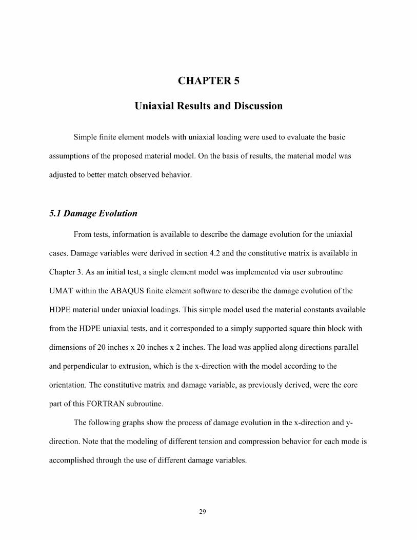
The following graphs show the process of damage evolution in the x-direction and y-

direction. Note that the modeling of different tension and compression behavior for each mode is

accomplished through the use of different damage variables.

30

0. 0000

0. 2000

0. 4000

0. 6000

0. 8000

1. 0000

1. 2000

0. 0004 0. 0024 0. 0044 0. 0064 0. 0084 0. 0104 0. 0124 0. 0144 0. 0164

St rai n

Dam

age

Varia

ble

Figure 5-1: Damage evolution for the HDPE material model with uniaxial tension loading parallel to extrusion

0. 0000

0. 2000

0. 4000

0. 6000

0. 8000

1. 0000

1. 2000

0. 0004 0. 0104 0. 0204 0. 0304 0. 0404 0. 0504

St rai n

Dam

age

Varia

ble

Figure 5-2: Damage evolution for the HDPE material model with uniaxial compression loading parallel to extrusion

31

-0.2

0

0.2

0.4

0.6

0.8

1

1.2

0 0.001 0.002 0.003 0.004 0.005 0.006

Strain

Dam

age

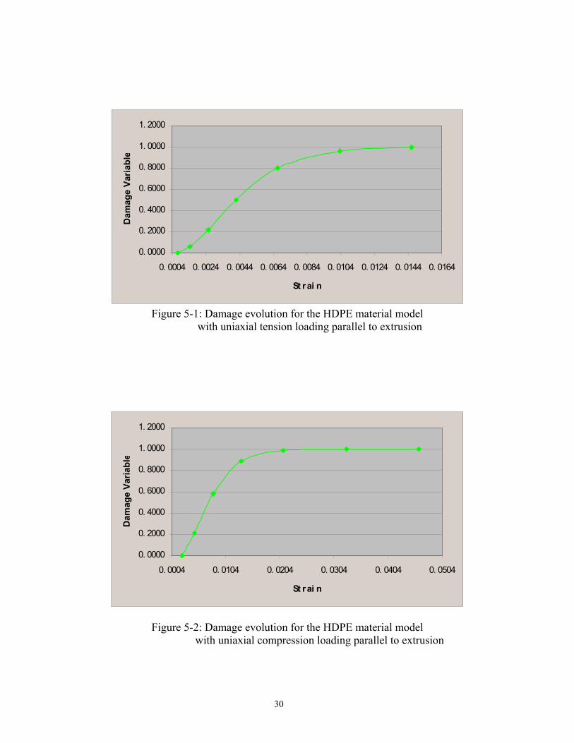
Figure 5-3: The damage and strain relation of the HDPE material model

with uniaxial tension perpendicular to extrusion

0

0.2

0.4

0.6

0.8

1

1.2

0.000 0.010 0.020 0.030 0.040 0.050

Strain

Dam

age

Figure 5-4: The damage and strain relation of the HDPE material model

with uniaxial compression perpendicular to extrusion

32

0

0. 2

0. 4

0. 6

0. 8

1

1. 2

0. 00E+00 5. 00E- 03 1. 00E- 02 1. 50E- 02 2. 00E- 02 2. 50E- 02

Shear St rai n

Dam

age

Leve

Damage Mode 1 Shear Damage Mode Damage Mode2

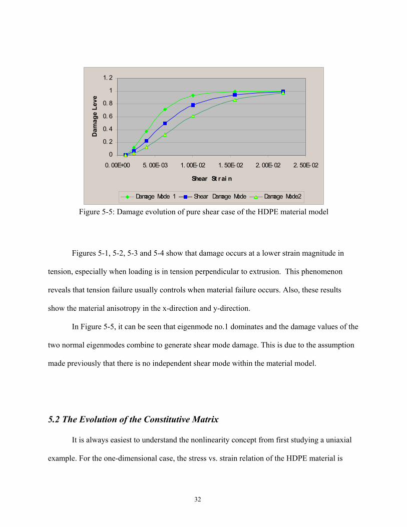
Figure 5-5: Damage evolution of pure shear case of the HDPE material model

Figures 5-1, 5-2, 5-3 and 5-4 show that damage occurs at a lower strain magnitude in

tension, especially when loading is in tension perpendicular to extrusion. This phenomenon

reveals that tension failure usually controls when material failure occurs. Also, these results

show the material anisotropy in the x-direction and y-direction.

In Figure 5-5, it can be seen that eigenmode no.1 dominates and the damage values of the

two normal eigenmodes combine to generate shear mode damage. This is due to the assumption

made previously that there is no independent shear mode within the material model.

5.2 The Evolution of the Constitutive Matrix

It is always easiest to understand the nonlinearity concept from first studying a uniaxial

example. For the one-dimensional case, the stress vs. strain relation of the HDPE material is

33

generalized as equations. Now that the material model must apply to the plane stress case, the

link between the stress domain and the strain domain is no longer a variable, but a tensor. Given

the constants obtained from uniaxial specimen tests, the damage evolution was described in

section 4.1. From the formulations in chapter 3, it is obvious that during the nonlinear damage

process the constitutive matrix of the HDPE material will vary as a result of the evolution of the

damage variables. To give an example, the same user material model described in section 5.1

was used here. Note again that the single element was subjected to a uniaxial loading in the x-

direction and the formulations and derivations mentioned in Chapters 3 and 4 are the

fundamentals of the material model. A whole process of the evolution of the constitutive matrix

accompanying the damage was then obtained, and it is shown in Appendix Tables A-9 and A-10

separately to distinguish tension and compression loading.

In these two tables, the damage variable shown is the one corresponding to eigenmode

no.1, because eigenmode no.1 represents the x-direction behavior of the HDPE material in this

case. Also, for tension and compression, different damage variables were used for eigenmode

no.1. The damage variable which corresponds to the other normal eigenmode is irrelevant in this

case. The results show that its value is too small to have a noticeable effect when the external

loads are applied along the x-direction.

From the results tabulated, it is found that, during the nonlinear damage process, the

constitutive matrix changes its components. If the external loading is parallel to extrusion, which

was defined as the x-direction in the ABAQUS UMAT subroutine, C11 experienced larger

changes compared to C22. This phenomenon is due to the fact that, within this model, the

34

damage variables )1(D and )2(D correspond to the normal eigenmodes, respectively. The

eigenmode one is related to the x-direction behavior, and the eigenmode two is related to the y-

direction behavior. The tabulated results reflect the x-direction behavior which is dominated by

)1(D . C11 is a function of )1(D , so from the table, it is observed that C11 controls the changes.

Although the results of loading in the y-direction are not listed, it can be concluded that if

the external loading is perpendicular to the grain, which is y-direction in the ABAQUS model,

changes in C22 will dominate the change in properties with respect to C11.

5.3 Uniaxial Behavior Modeling

This material model was calibrated with the uniaxial test results. To get the uniaxial

stress vs. strain relations, the same user material model described in section 5.1 was used. Again,

the formulations and derivations mentioned in Chapters 3 and 4 are the fundamentals of the

material model. The results are shown in Figure 5-6, labeled as the “CDM result”. From the

figure, the results do not match those of experiment in that the response indicates abrupt

softening, followed by a leveling off. For the case of tension parallel to extrusion, stress in the

test specimen rises rapidly with strain and then levels off in a region that appears plastic in its

behavior. Thus, the material model, as derived in Chapter 4 on the basis of the theory of

Continuum Damage Mechanics, does not exhibit the apparent plastic behavior observed in the

tests. One may observe that the growth of damage causes a reduction in both tangent stiffness

and existing stress. The latter causes strain softening, which does not allow for the stress plateau

35

that was observed experimentally. To better model the experimental behavior, the model was

adjusted in two ways.

First, to represent the apparent plastic behavior, the term representing the reduction in

existing stress was removed. Essentially, given the definition of damage evolution that was used,

this simply ensures that the stress-strain relationship follows the hyperbolic tangent curve by

using the tangent stiffness. Then, a second set of damage parameters was introduced to replace

the terms removed and cause softening, but only after a critical value of strain has been reached.

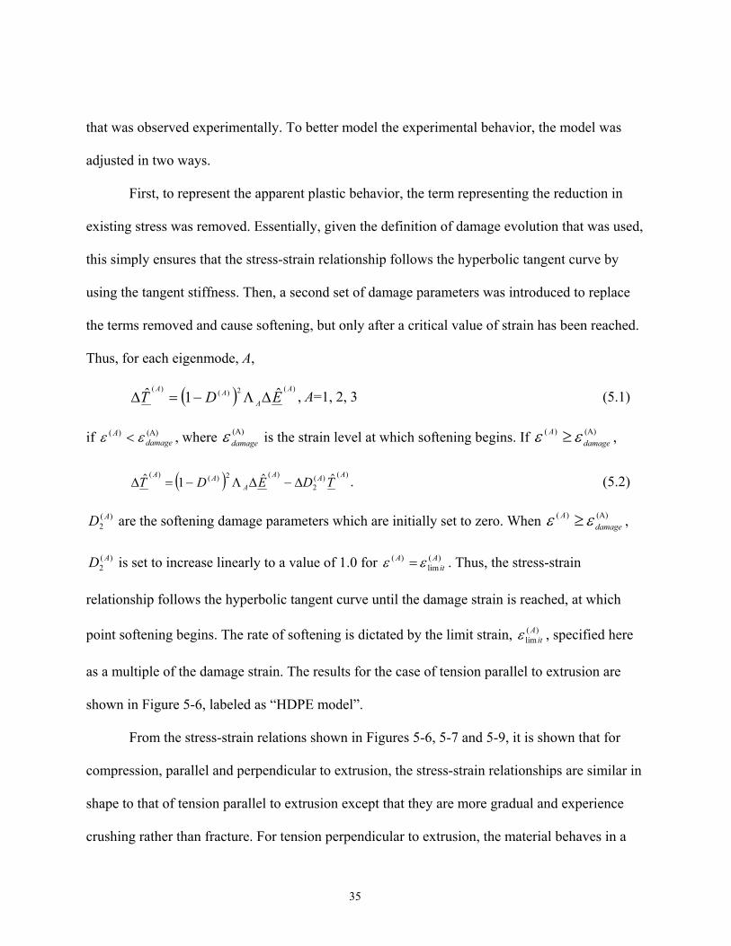
Thus, for each eigenmode, A,

( ) )(2)()( ˆ1ˆ A

AAA

EDT ∆Λ−=∆ , A=1, 2, 3 (5.1)

if (A))(damage

A εε < , where (A)damageε is the strain level at which softening begins. If (A))( damage

A εε ≥ ,

( ) )()(2

)(2)()( ˆˆ1ˆ AAA

AAA

TDEDT ∆−∆Λ−=∆ . (5.2)

)(2

AD are the softening damage parameters which are initially set to zero. When (A))( damageA εε ≥ ,

)(2

AD is set to increase linearly to a value of 1.0 for )(lim

)( Ait

A εε = . Thus, the stress-strain

relationship follows the hyperbolic tangent curve until the damage strain is reached, at which

point softening begins. The rate of softening is dictated by the limit strain, )(lim

Aitε , specified here

as a multiple of the damage strain. The results for the case of tension parallel to extrusion are

shown in Figure 5-6, labeled as “HDPE model”.

From the stress-strain relations shown in Figures 5-6, 5-7 and 5-9, it is shown that for

compression, parallel and perpendicular to extrusion, the stress-strain relationships are similar in

shape to that of tension parallel to extrusion except that they are more gradual and experience

crushing rather than fracture. For tension perpendicular to extrusion, the material behaves in a

36

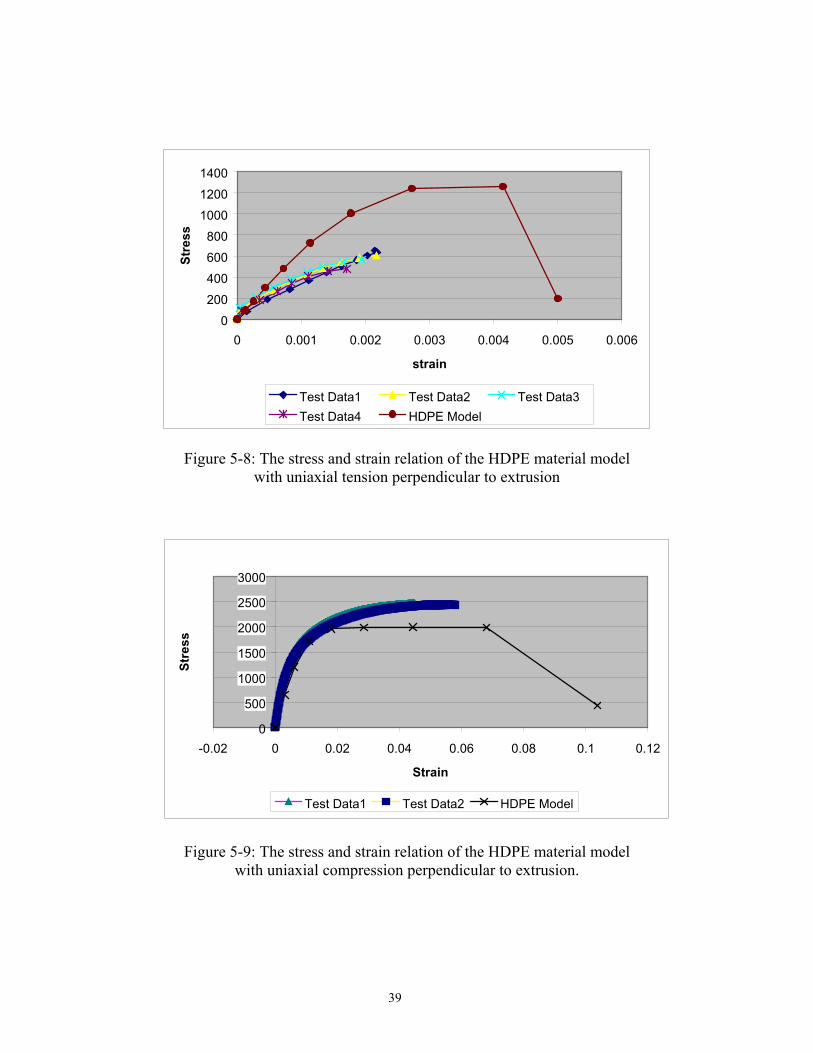
brittle manner. The stress-strain relationship matches the hyperbolic tangent function only until

failure occurs suddenly at a relatively low strain value. In Figure 5-8, the experimental and

numerical results are somewhat different. The experimental data and the values of the constants,

a and b, were taken from past work (Lockyear, 2000). Close inspection of the experimental data

shows that, in all cases for tension perpendicular to extrusion, specimens were initially subjected

to compressive force before being loaded in tension. In Figure 5-8, the experimental points have

been shifted horizontally to approximately pass through the origin and the negative points have

been discarded. However, the curve that was fit to the data does not take into account the vertical

shift and, thus, appears to be somewhat high. Modification of existing constants was beyond the

scope of this work, however.

Figures 5-6 through 5-9 show softening behavior in the material. However, the curves in

Figure 5-7 require explanation. If the specimen is free to expand, the lateral strain, perpendicular

to extrusion, attains failure during compressive loading parallel to extrusion. If expansion is

restrained, softening failure results from material crushing. For the direction perpendicular to

extrusion, tensile softening properties were set from both previously mentioned tests (labeled as

orthotropic damage) and from the assumption that they are the same as those parallel to

extrusion, for reasons described subsequently. The actual test specimen was a relatively large

extruded section with a complicated pattern of lateral restraint, which eventually exhibited brittle

failure. This type of complex behavior could not be simulated well with a single-element model.

Table 5-1 shows the damage strain magnitude related to each eigenmode. These values

were obtained from uniaxial tests. Failure data for all of the tests were predictable and repeatable

except for those in tension perpendicular to extrusion, as given in Table 5-2. Because of the large

37

amount of scatter in the data, average values for only cases T90o-2, T90o-3, T90o-4, and T90o-5

were used.

Damage strain

Uniaxial tension parallel to grain 0.0146

Uniaxial compression parallel to grain 0.0459

Uniaxial tension perpendicular to grain 0.00255

Uniaxial compression perpendicular to grain 0.0461

Table 5-1: The damage strain related to eigenmodes

Specimen No. Constant a Constant b Damage strain

T90°-1 1534 250 0.0023630

T90°-2 855 639 0.0026570

T90°-3 763 703 0.0022950

T90°-4 672 854 0.0020810

T90°-5 885 595 0.0031540

T90°-6 456 1190 0.0016910

Average Values Used 794 699 0.002547

Standard Derivation 42.30% 43.93% 21.04%

Table 5-2: Test data with uniaxial loading perpendicular to the grain (Lockyear, 1999)

38

0200400600800

100012001400

0 0.01 0.02 0.03 0.04

Strain

Stre

ss

HDPE Model Test Data1 Test Data2 CDM result

Figure 5-6: The stress and strain relation of the HDPE material model with uniaxial tension parallel to extrusion.

0500

10001500200025003000

0 0.01 0.02 0.03 0.04 0.05

Strain

Stre

ss (p

si)

Test Data1 Test Data2HDPE Model, Isotropic Damage HDPE Model, Orthotropic DamageHDPE Model, Confined

Figure 5-7: The stress and strain relation of the HDPE material model with uniaxial compression parallel to extrusion.

39

0200400600800

100012001400

0 0.001 0.002 0.003 0.004 0.005 0.006

strain

Stre

ss

Test Data1 Test Data2 Test Data3Test Data4 HDPE Model

Figure 5-8: The stress and strain relation of the HDPE material model with uniaxial tension perpendicular to extrusion

0

500

1000

1500

2000

2500

3000

-0.02 0 0.02 0.04 0.06 0.08 0.1 0.12

Strain

Stre

ss

Test Data1 Test Data2 HDPE Model

Figure 5-9: The stress and strain relation of the HDPE material model with uniaxial compression perpendicular to extrusion.

40

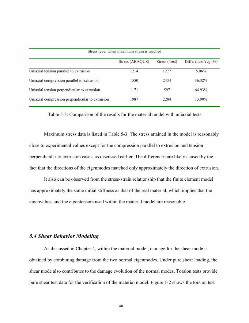
Stress level when maximum strain is reached

Stress (ABAQUS) Stress (Test) Difference/Avg (%)

Uniaxial tension parallel to extrusion 1214 1277 5.06%

Uniaxial compression parallel to extrusion 1550 2434 36.32%

Uniaxial tension perpendicular to extrusion 1171 597 64.93%

Uniaxial compression perpendicular to extrusion 1987 2284 13.90%

Table 5-3: Comparison of the results for the material model with uniaxial tests

Maximum stress data is listed in Table 5-3. The stress attained in the model is reasonably

close to experimental values except for the compression parallel to extrusion and tension

perpendicular to extrusion cases, as discussed earlier. The differences are likely caused by the

fact that the directions of the eigenmodes matched only approximately the direction of extrusion.

It also can be observed from the stress-strain relationship that the finite element model

has approximately the same initial stiffness as that of the real material, which implies that the

eigenvalues and the eigentensors used within the material model are reasonable.

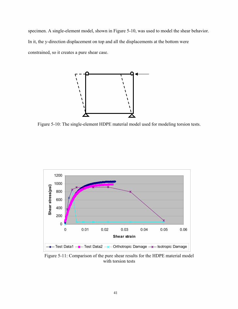
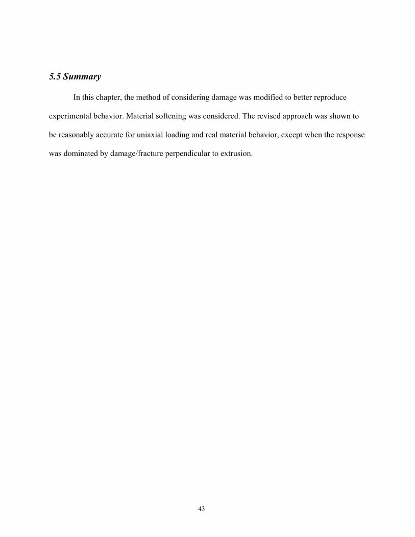
5.4 Shear Behavior Modeling

As discussed in Chapter 4, within the material model, damage for the shear mode is

obtained by combining damage from the two normal eigenmodes. Under pure shear loading, the

shear mode also contributes to the damage evolution of the normal modes. Torsion tests provide

pure shear test data for the verification of the material model. Figure 1-2 shows the torsion test

41

specimen. A single-element model, shown in Figure 5-10, was used to model the shear behavior.

In it, the y-direction displacement on top and all the displacements at the bottom were

constrained, so it creates a pure shear case.

Figure 5-10: The single-element HDPE material model used for modeling torsion tests.

0

200

400

600

800

1000

1200

0 0.01 0.02 0.03 0.04 0.05 0.06

Shear strain

Shea

r str

ess(

psi)

Test Data1 Test Data2 Orthotropic Damage Isotropic Damage

Figure 5-11: Comparison of the pure shear results for the HDPE material model with torsion tests

42

Maximum stress level when maximum strain is reached (psi)

Stress (ABAQUS) Stress (Torsion Test) Difference/Avg (%)

Pure Shear 914 1006 9.15%

Table 5-4: Comparison of the max shear stress for the HDPE material model and torsion tests

From Figure 5-11, the experimental and numerical curves are quite different when the

given uniaxial data is used. The softening/failure shown in the model at such an early stage in the

analysis is caused by the assumed brittleness of the material when subjected to tension

perpendicular to extrusion, labeled as the Orthotropic Damage case. However, experimental

observations indicated failure by fracture on planes of 45 degrees. The experimental behavior is

inconsistent with the assumption of the weak/brittle plane perpendicular to extrusion that was

assumed in the model. If the weakness is removed and the tension properties are assumed to be

the same both parallel and perpendicular to extrusion, labeled as the Isotropic Damage case, the

experimental and numerical curves are similar. The early fracture failure from analyses of both

the torsion test and the compression test parallel to extrusion point out the inconsistency between

the tension tests perpendicular to extrusion and the others. Further tests should be conducted to

reconcile these differences, but testing is beyond the scope of this work.

43

5.5 Summary

In this chapter, the method of considering damage was modified to better reproduce

experimental behavior. Material softening was considered. The revised approach was shown to

be reasonably accurate for uniaxial loading and real material behavior, except when the response

was dominated by damage/fracture perpendicular to extrusion.

44

CHAPTER 6

Biaxial Results and Discussion

The proposed material model has been shown to reasonably reproduce the behavior of the

HDPE material for uniaxial loading. One of the objectives of this research is to determine how

the material model presented in this thesis performs for more general applications. The Iosipescu

and Five-point bending tests provided some biaxial data with which the material model could be

compared.

6.1 Iosipescu Shear Test

The Iosipescu shear test (ASTM D5379) is a standard test to determine the shear strength

of materials. Figure 6-1 shows the test setup for the Iosipescu test. The test fixture consists of

two parts that clamp the specimen. Load is applied to one of the parts, which is allowed to slide

vertically, enforcing shear in the notch of the specimen. Detailed descriptions of this test can be

found in ASTM D 5379 and the report of Haiar (2000).

Figure 6-2 shows the Iosipescu test model with boundary conditions within ABAQUS

finite element software. The specimen is a 3 inch x 0.75 inch x 0.3 inch block with a 90- degree

notch on each edge. Specific dimensions and boundary conditions can be found in ASTM D5379

(1998). For the finite element model, nodes representing the surfaces of the specimen subject to

load from the fixture were constrained to move vertically.

45

Figure 6-1: Iosipescu shear test setup

Figure 6-2: The Iosipescu shear test model with ABAQUS

46

For this model, cases for both orthotropic damage (i.e., weak in tension perpendicular to

extrusion) and isotropic damage were considered. Load and deflection data, as well as softening

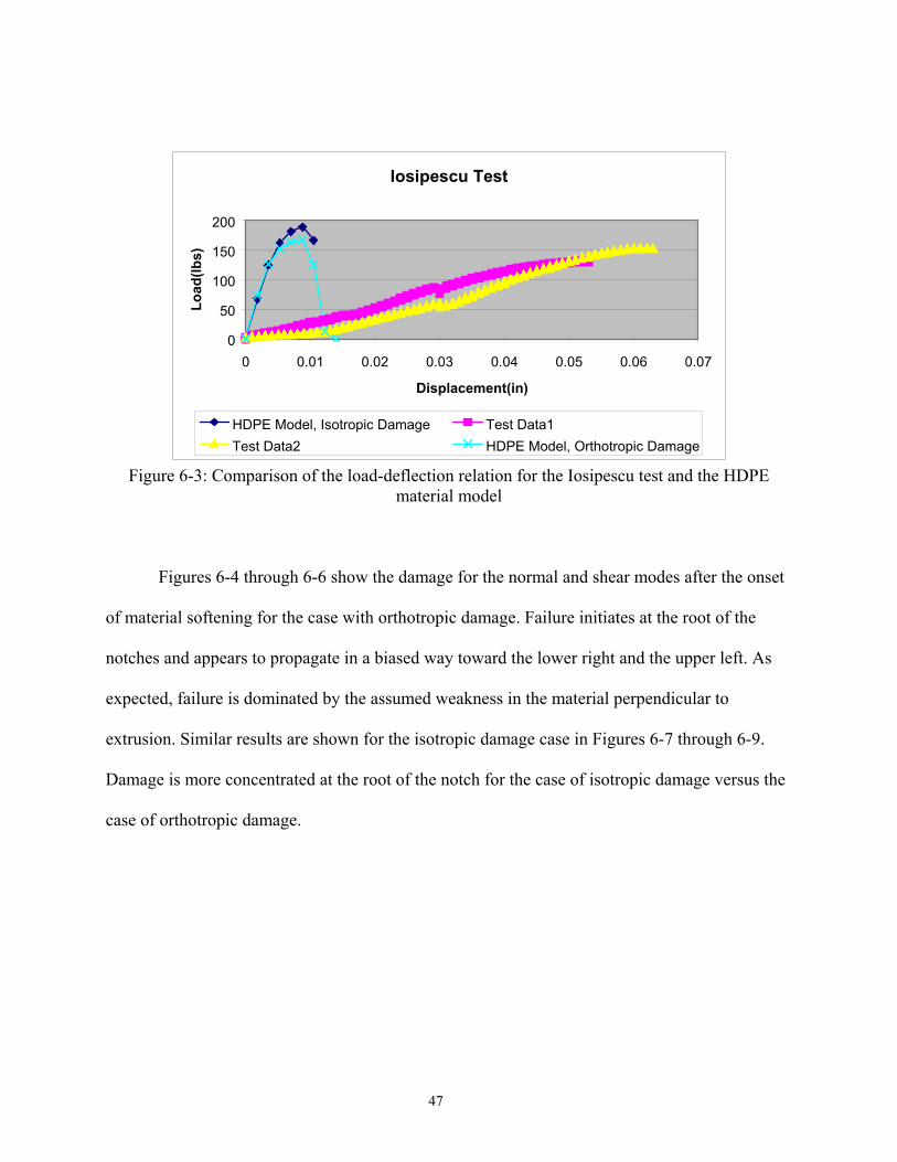
damage and strain were examined. Load versus deflection data are shown in Figure 6-3. It is

observed from the figure that, when failure occurs, the Iosipescu model achieves a maximum

strength level that is close to that of test results for both cases. The maximum strength results are

tabulated in Table 6-1. The load-deflection relationship shows material softening, with a reduced

failure strength for the orthotropic damage case compared to that of the isotropic damage case.

The load-deflection result of the Iosipescu specimen analysis shows that the finite

element model is very stiff compared with the test, even at the very beginning of the analysis.

However, in the uniaxial analyses of the previous chapter, the stiffness of the model agreed quite

well with test results, especially in the early stages of loading. Therefore, one may speculate that

the large difference in displacement data is the result of a lack of agreement in the items being

compared, such as additional effects of flexibility in the test fixture or local deformation in the

specimen. Indeed, the Iosipescu test setup is relatively complex, while the finite element model

was simple.

47

Iosipescu Test

0

50

100

150

200

0 0.01 0.02 0.03 0.04 0.05 0.06 0.07

Displacement(in)

Load

(lbs)

HDPE Model, Isotropic Damage Test Data1Test Data2 HDPE Model, Orthotropic Damage

Figure 6-3: Comparison of the load-deflection relation for the Iosipescu test and the HDPE

material model

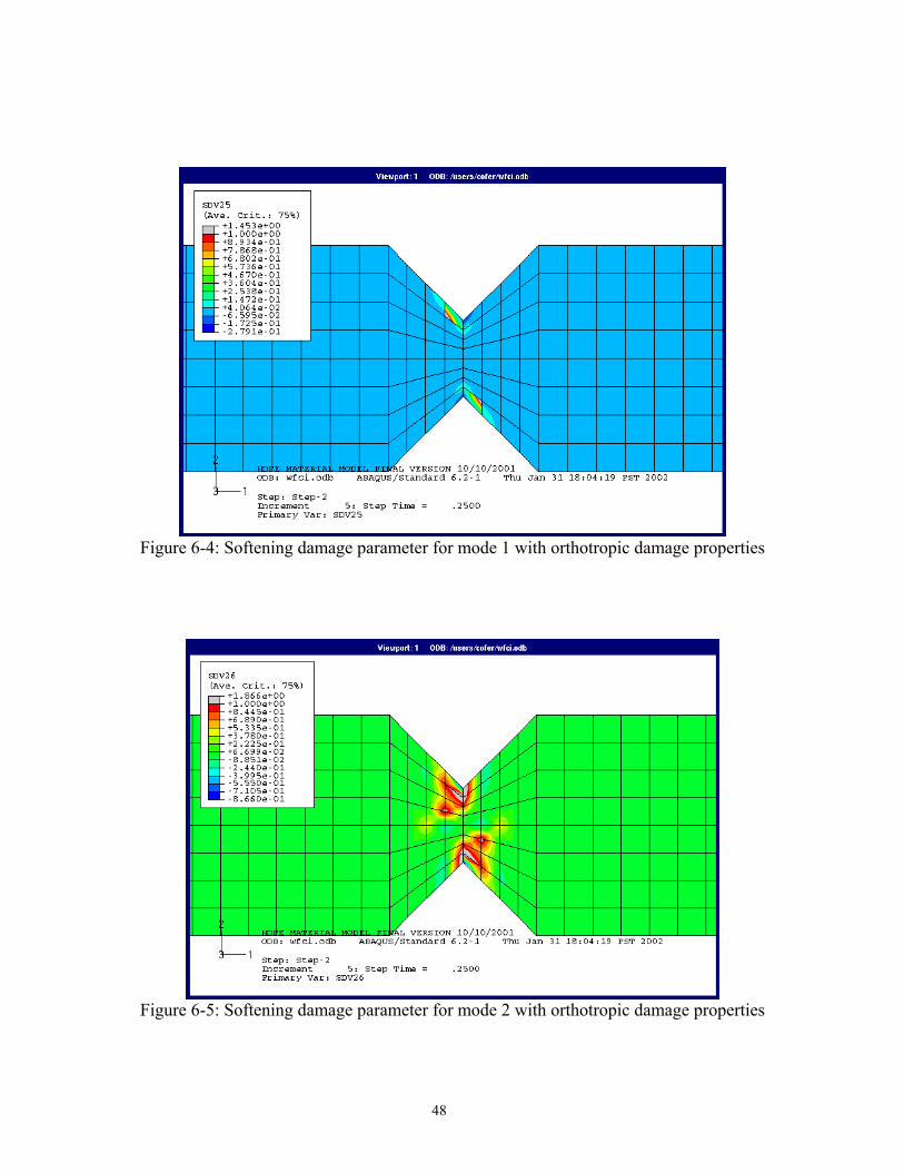
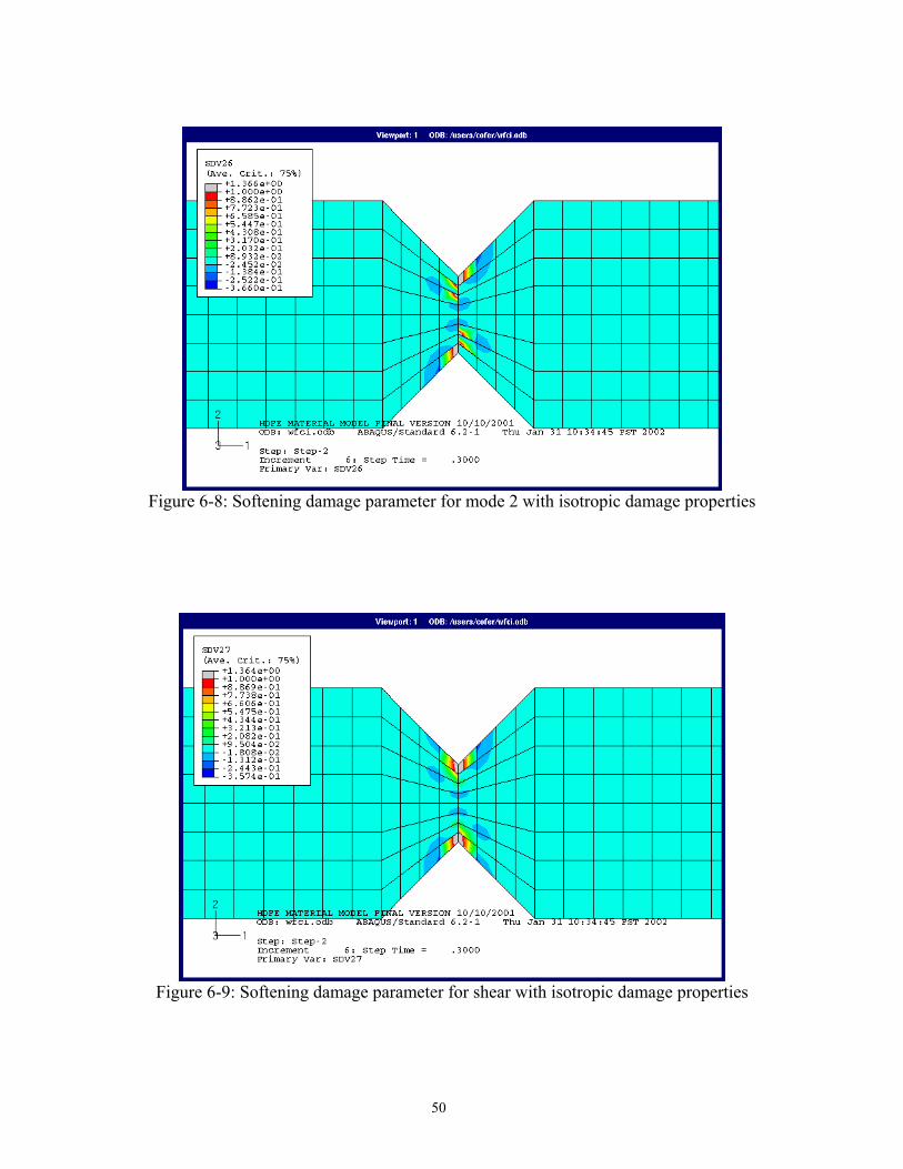
Figures 6-4 through 6-6 show the damage for the normal and shear modes after the onset

of material softening for the case with orthotropic damage. Failure initiates at the root of the

notches and appears to propagate in a biased way toward the lower right and the upper left. As

expected, failure is dominated by the assumed weakness in the material perpendicular to

extrusion. Similar results are shown for the isotropic damage case in Figures 6-7 through 6-9.

Damage is more concentrated at the root of the notch for the case of isotropic damage versus the

case of orthotropic damage.

48

Figure 6-4: Softening damage parameter for mode 1 with orthotropic damage properties

Figure 6-5: Softening damage parameter for mode 2 with orthotropic damage properties

49

Figure 6-6: Softening damage parameter for shear with orthotropic damage properties

Figure 6-7: Softening damage parameter for mode 1 with isotropic damage properties

50

Figure 6-8: Softening damage parameter for mode 2 with isotropic damage properties

Figure 6-9: Softening damage parameter for shear with isotropic damage properties

51

Figures 6-10 and 6-11 show the principal strain pattern for the Iosipescu model with

orthotropic damage properties at the point of maximum strength and at failure, respectively. The

red arrows denote maximum tensile strain while the yellow arrows show maximum compressive

strain. Prior to softening, shown in Figure 6-10, the strain is concentrated in the region between

the notches and, in that location, it is primarily shear strain. After softening, shown in Figure 6-

11, the strain becomes highly concentrated. One may note that the strain values shown in Figure

6-11 are much greater than those of Figure 6-10. Because the large strains occur in elements

subject to damage and softening, their values may be unreliable. However, the maximum tensile

strains occur at the root of the notches, oriented at an angle of 45 degrees, and they are nearly

uniaxial. Away from the root of the notches, the tensile strains are oriented vertically with

corresponding horizontal compressive strains, indicating shear.

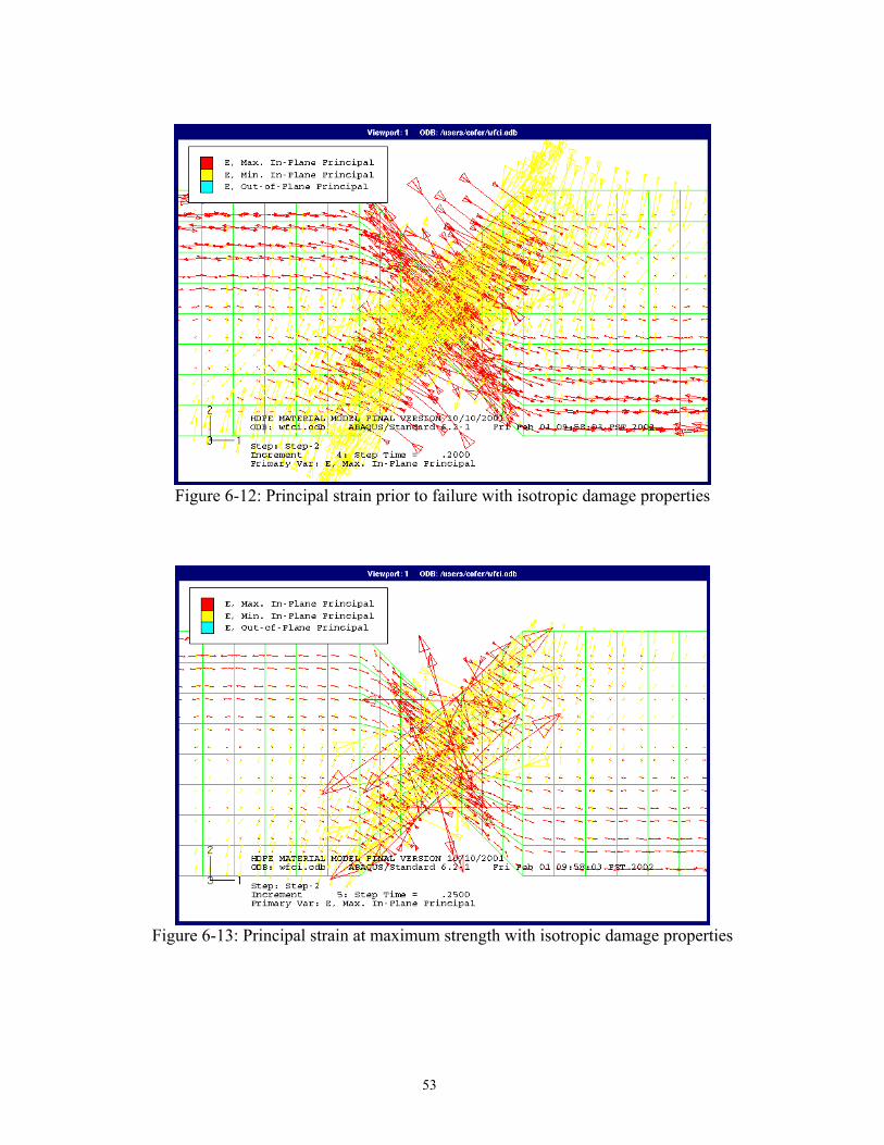
Principal strain for the last three steps of the analysis of the Iosepescu model with

isotropic damage properties is shown in Figures 6-12 through 6-14. Figure 6-12 represents the

step prior to that of maximum strength. As with the case of orthotropic damage properties, the

strain is concentrated between the notches, and it is dominated by shear. In Figure 6-13,

representing the state of maximum strength, high strain has begun to localize. The strain state at

softening is shown in Figure 6-14.

52

Figure 6-10: Principal strain at maximum strength with orthotropic damage properties

Figure 6-11: Principal strain at failure with orthotropic damage properties

53

Figure 6-12: Principal strain prior to failure with isotropic damage properties

Figure 6-13: Principal strain at maximum strength with isotropic damage properties

54

Figure 6-14: Principal strain at failure with isotropic damage properties

Maximum Iosipescu strength when failure occurs

Maximum Load Applied (lbs)

Finite Element Model, Orthotropic Damage 167.8

Finite Element Model, Isotropic Damage 189.4

Iosipescu Tests 146.5

Table 6-1: Comparison of the maximum strength for the material model with Iosipescu tests

6.2 Five-point beam shear bending test

Many marine fender systems are subject to bending-shear. The biaxial behavior of the

HDPE material model can be investigated by modeling the five-point beam shear bending test.

55

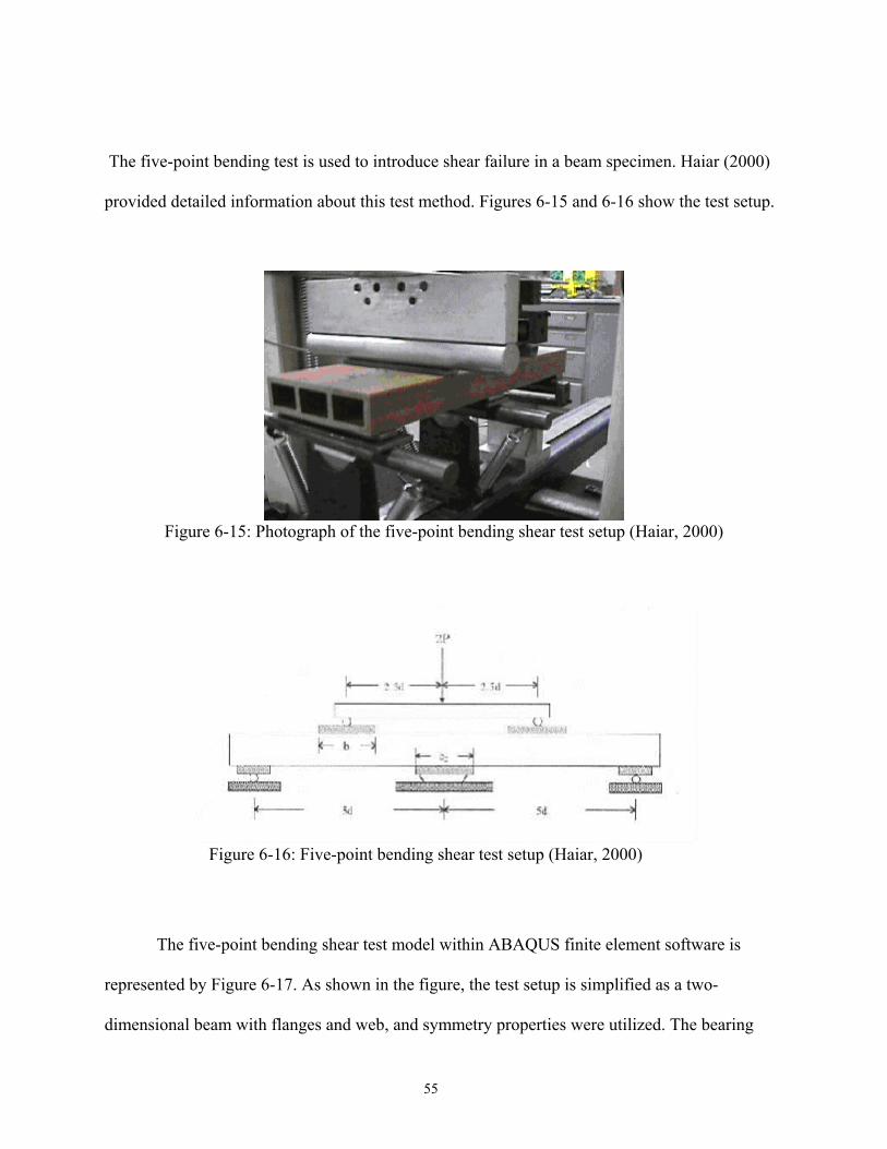
The five-point bending test is used to introduce shear failure in a beam specimen. Haiar (2000)

provided detailed information about this test method. Figures 6-15 and 6-16 show the test setup.

Figure 6-15: Photograph of the five-point bending shear test setup (Haiar, 2000)

Figure 6-16: Five-point bending shear test setup (Haiar, 2000)

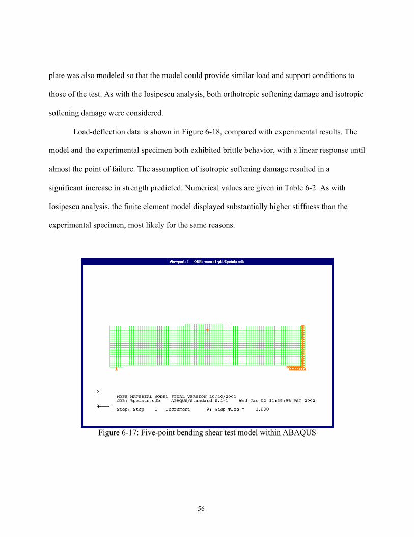
The five-point bending shear test model within ABAQUS finite element software is

represented by Figure 6-17. As shown in the figure, the test setup is simplified as a two-

dimensional beam with flanges and web, and symmetry properties were utilized. The bearing

56

plate was also modeled so that the model could provide similar load and support conditions to

those of the test. As with the Iosipescu analysis, both orthotropic softening damage and isotropic

softening damage were considered.

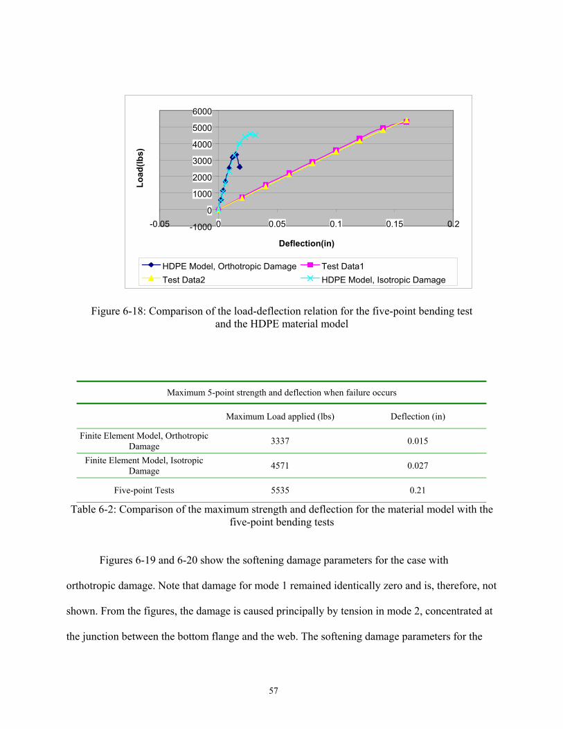
Load-deflection data is shown in Figure 6-18, compared with experimental results. The

model and the experimental specimen both exhibited brittle behavior, with a linear response until

almost the point of failure. The assumption of isotropic softening damage resulted in a

significant increase in strength predicted. Numerical values are given in Table 6-2. As with

Iosipescu analysis, the finite element model displayed substantially higher stiffness than the

experimental specimen, most likely for the same reasons.

Figure 6-17: Five-point bending shear test model within ABAQUS

57

-1000

0

1000

2000

3000

4000

5000

6000

-0.05 0 0.05 0.1 0.15 0.2

Deflection(in)

Load

(lbs)

HDPE Model, Orthotropic Damage Test Data1Test Data2 HDPE Model, Isotropic Damage

Figure 6-18: Comparison of the load-deflection relation for the five-point bending test and the HDPE material model

Maximum 5-point strength and deflection when failure occurs

Maximum Load applied (lbs) Deflection (in)

Finite Element Model, Orthotropic Damage 3337 0.015

Finite Element Model, Isotropic Damage 4571 0.027

Five-point Tests 5535 0.21

Table 6-2: Comparison of the maximum strength and deflection for the material model with the five-point bending tests

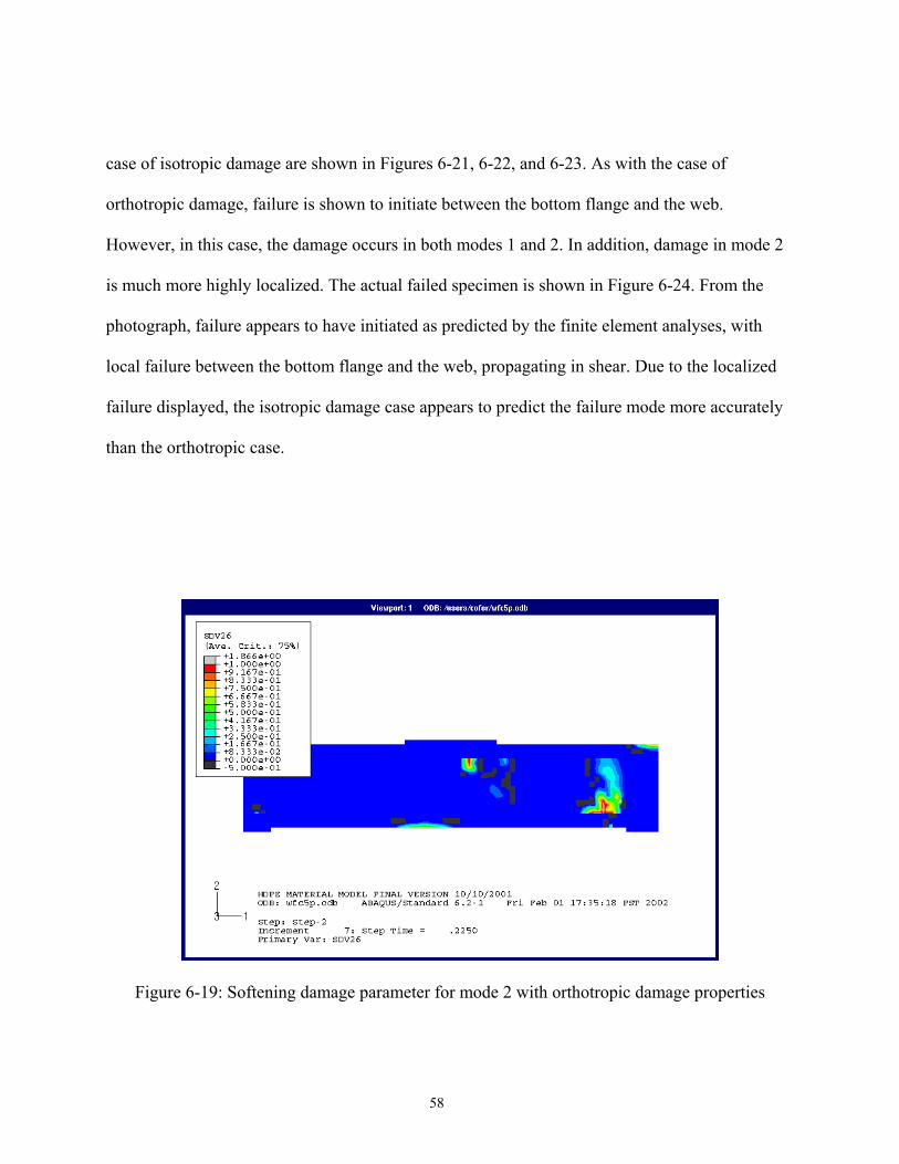
Figures 6-19 and 6-20 show the softening damage parameters for the case with

orthotropic damage. Note that damage for mode 1 remained identically zero and is, therefore, not

shown. From the figures, the damage is caused principally by tension in mode 2, concentrated at

the junction between the bottom flange and the web. The softening damage parameters for the

58

case of isotropic damage are shown in Figures 6-21, 6-22, and 6-23. As with the case of

orthotropic damage, failure is shown to initiate between the bottom flange and the web.

However, in this case, the damage occurs in both modes 1 and 2. In addition, damage in mode 2

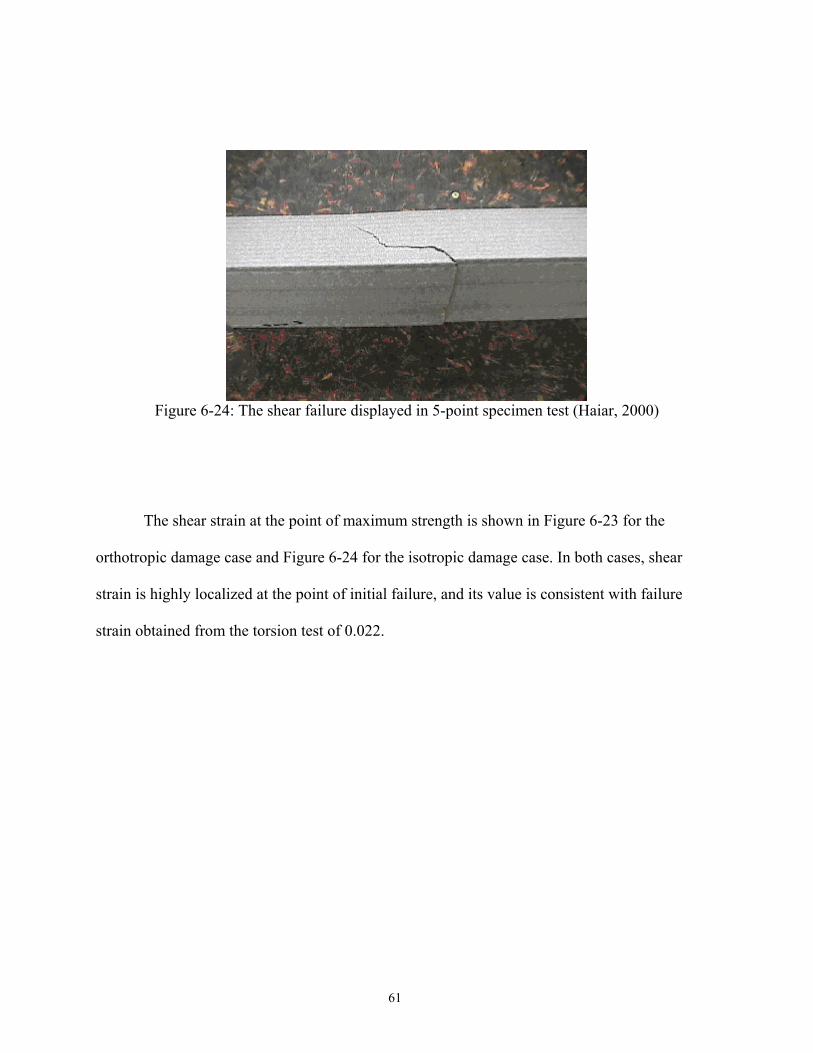
is much more highly localized. The actual failed specimen is shown in Figure 6-24. From the

photograph, failure appears to have initiated as predicted by the finite element analyses, with

local failure between the bottom flange and the web, propagating in shear. Due to the localized

failure displayed, the isotropic damage case appears to predict the failure mode more accurately

than the orthotropic case.

Figure 6-19: Softening damage parameter for mode 2 with orthotropic damage properties

59

Figure 6-20: Softening damage parameter for shear with orthotropic damage properties

Figure 6-21: Softening damage parameter for mode 1 with isotropic damage properties

60

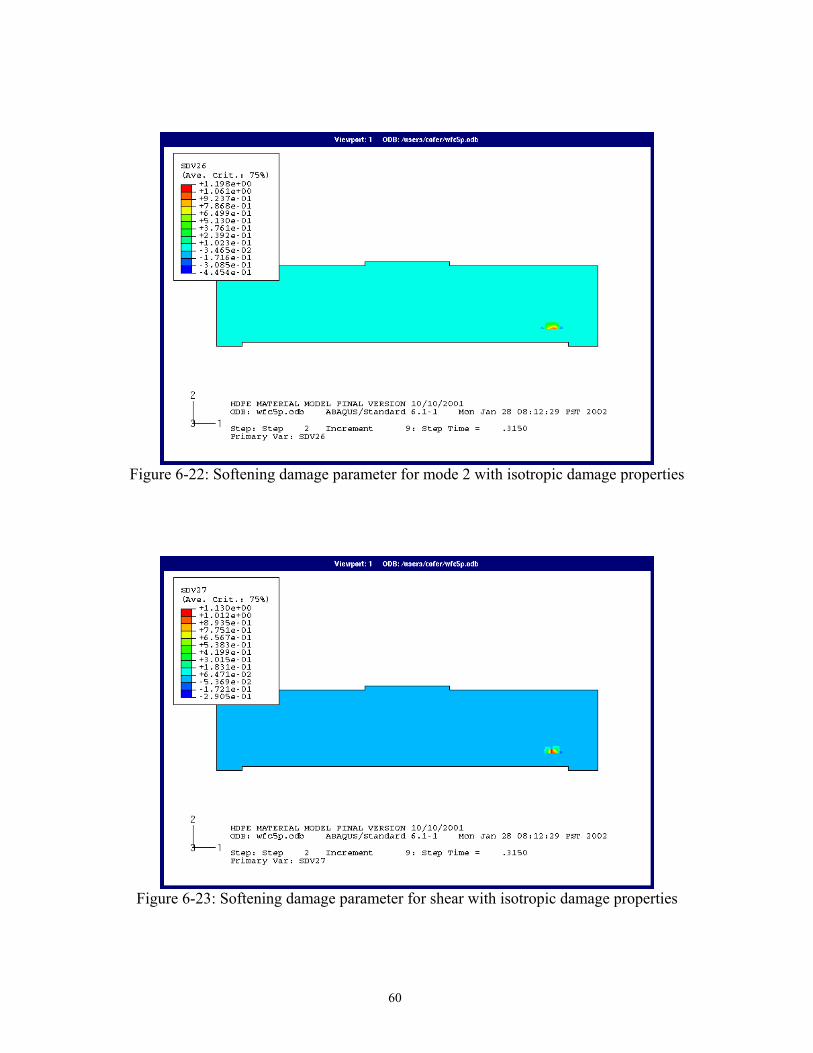
Figure 6-22: Softening damage parameter for mode 2 with isotropic damage properties

Figure 6-23: Softening damage parameter for shear with isotropic damage properties

61

Figure 6-24: The shear failure displayed in 5-point specimen test (Haiar, 2000)

The shear strain at the point of maximum strength is shown in Figure 6-23 for the

orthotropic damage case and Figure 6-24 for the isotropic damage case. In both cases, shear

strain is highly localized at the point of initial failure, and its value is consistent with failure

strain obtained from the torsion test of 0.022.

62

Figure 6-25: Shear strain at maximum strength with orthotropic damage properties

Figure 6-26: Shear strain at maximum strength with isotropic damage properties

63

From Table 6-2 and Figure 6-18, it is observed that the finite element model of the five-

point bending shear test predicted a maximum load that is smaller than that of test results.

However, the failure mode matched experimental observations, which is encouraging. From the

distribution of strain and softening damage, the model with isotropic damage properties

reproduced the material behavior in a more accurate way than the model with orthotropic

damage properties.

6.3 Summary

Results of the Iosipescu test and the five-point bending test were presented in this chapter

to evaluate the ability of the model to accurately reproduce the biaxial behavior of the HDPE

wood-composite material. In both models, displacement values were substantially lower than

those measured in tests. This may be a result of local crushing effects, flexibility within the test

fixtures, or a lack of agreement between displacements measured. For the Iosipescu test,

especially, the boundary conditions and loading were difficult to reproduce. It was shown from

the five-point strain and damage contours that, like the photo of the specimen shown, when the

specimen reaches the failure limit, there is an in-plane region having the same shape as the

cracks in the real specimen. In addition, the failure load values were fairly close to experiment,

with that from the Iosipescu test being higher and that from the five-point test being lower.

64

CHAPTER 7

Conclusion

In this thesis, a new material model for HDPE wood-plastic material is presented. Briefly,

it can be noticed that three important components were used to realize the objectives of the

material model. The first is the concept of effective stress, which is used to build the link

between the damaged state and undamaged state of a material point. The second is the idea of the

decomposition of the elastic tensor, which is used as a means to include the effect of anisotropy.

Three modes were decomposed from the plane stress tensor used within the two-dimensional

HDPE material model. Finally, the hyperbolic-tangent shape of the HDPE stress-strain relations

is the basis of this material model. Based upon the shape similarity of the stress-strain relations

obtained from different tests, the assumption was made that damage caused the nonlinearity of

the HDPE material. From the hyperbolic-tangent shape, damage was derived in the form of a

scalar, and each damage variable was set to correspond to an eigenmode derived from elastic

tensor decomposition. The assumption was made that the first two eigenmodes could be related

to the uniaxial behavior of the HDPE material and that the shear mode behavior is influenced by

the two normal eigenmodes.

Separate damage variables were used for tension strain and compression strain within

each eigenmode of the material model, by which material anisotropy in tension and compression

could be modeled, as displayed in tests. The idea of volumetric strain was used to distinguish

whether an eigenmode at a material point is in tension or in compression. The constitutive

65

relation takes the form of a function of damage to describe nonlinear stress-strain relations. The

failure criteria of the HDPE material are proposed as strain-based.

Although the basic derivations were based on energy concepts, the material model was

adjusted to better match experimental behavior. First, separate damage parameters for each mode

were introduced to allow both material nonlinearity and softening/failure. Also, a means to

define damage in the shear mode in terms of damage in the normal modes was devised. Finally, a

scheme to relate damage in the normal modes to shear strain was implemented.

After implementing the theory of the material model into the finite element software

ABAQUS with user subroutine UMAT, small uniaxial models were analyzed for comparison

with tests. The results indicated that the use of tensile properties from tests in the direction

perpendicular to extrusion, which showed very brittle behavior compared to other directions, did

not lead to a consistent failure mode in the case of pure shear, which indicated nearly isotropic

behavior. Thus, for all subsequent analyses, both orthotropic and isotropic damage cases were

considered. In general, the isotropic cases yielded more accurate results than the orthotropic

cases.

Iosipescu shear and five-point bending tests were also modeled by the use of this material

model. The load-deflection curves of the Iosipescu and five-point model results indicated that the

finite element model was quite stiff in comparison with experimental results. However, because

stiffness of the simple uniaxial models closely matched experimental data, the apparent

differences in stiffness for the complicated tests are thought to result from issues of load

application and support in the models. The specimen strength values predicted in the models

were fairly close to those of experiment and the failure modes were similar.

66

The work of this thesis raised several questions and pointed to the need for further

research. Currently, the material model has no provision for reversal of strain. Even for

monotonic loading, local areas of a finite element model will unload as other areas soften and

fail. Also, logic needs to be introduced to consider cases in which, at an eigenmode for a material

point, the strain changes from tension to compression or vice versa.

The use of volumetric strain to indicate whether the state of strain for an eigenmode is

tensile or compressive needs to be investigated further. The idea was to use a strain invariant.

Another possibility would be to consider principal strain values. Similarly, the logic used to

assign damage to eigenmodes 1 and 2 on the basis of shear strain seemed to work reasonably

well in spite of the fact that it violates the assumption that the eigenmodes do not interact.

Interestingly, Arramon, et al. (2000) augmented the failure surface for their material model with

a provision for principal stress. Perhaps, a condition on principal strain could be devised to better

consider the interaction of shear and damage.

The performance of this material model in biaxial states of strain has not been tested

conclusively due to the lack of biaxial test data. With such data, a failure surface in stress space

could be plotted, evaluated, and compared to those of other materials and material models,

leading to more definite conclusions.

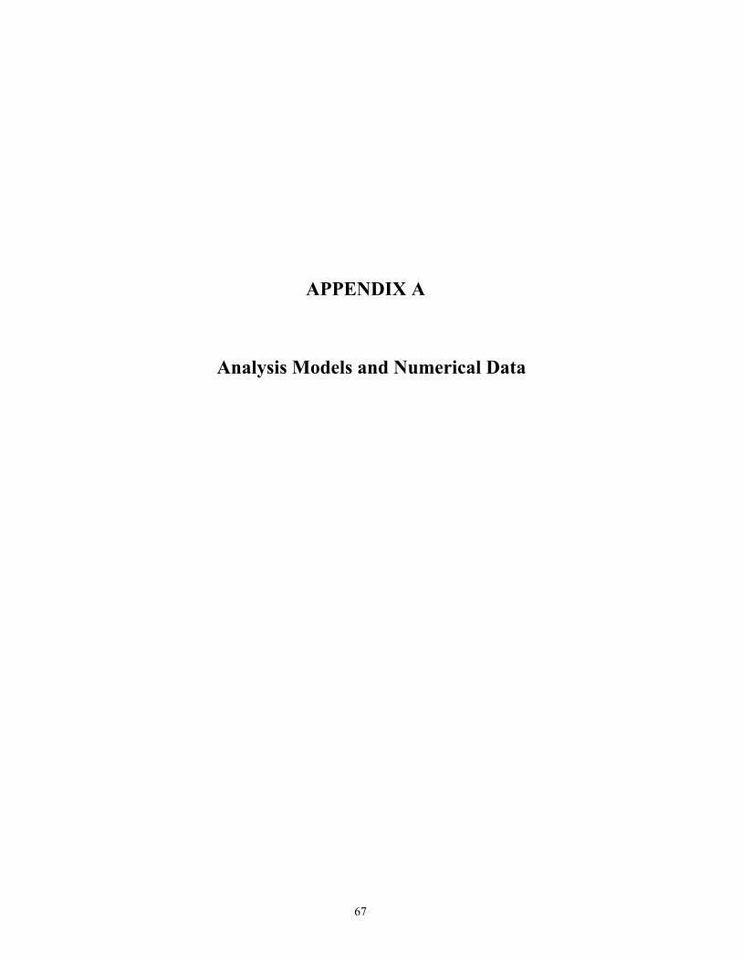
67

APPENDIX A

Analysis Models and Numerical Data

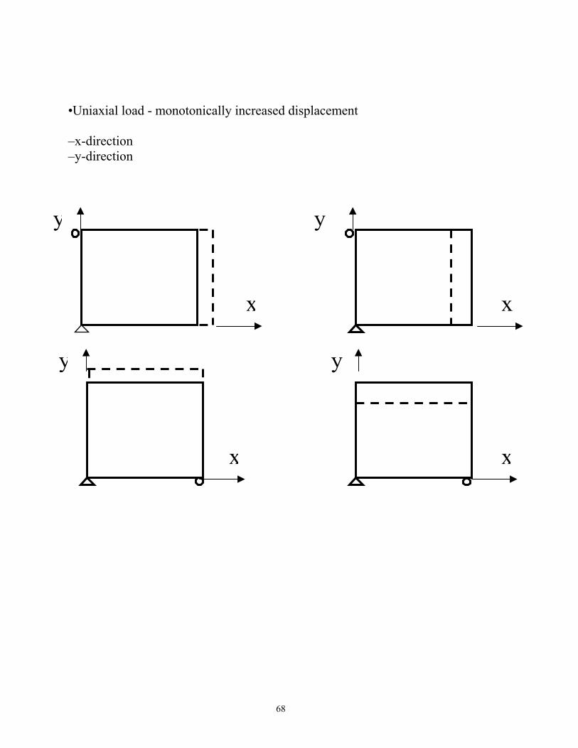
68

•Uniaxial load - monotonically increased displacement –x-direction –y-direction

x

y

x

y

x

y

x

y

69

Uniaxial tension parallel to grain

Stress (psi) Strain(in/in) 0 0

293 6.00E-04 590 1.20E-03 918 2.10E-03 1151 3.45E-03 1211 5.48E-03 1214 8.51E-03 1214 1.31E-02 1214 1.99E-02

3 3.00E-02

Table A-1: Abaqus stress-strain results with uniaxial tension parallel to grain

Uniaxial compression parallel to grain Strain (in/in) Stress (psi)

Orthotropic Damage Stress (psi)

Isotropic Damage Stress (psi)

Confined with Isotropic Damage

0 0 0 0 3.00E-07 0.1465 0.1465 0.1586 7.50E-04 299.7 299.7 327.1 1.50E-03 555.1 555.1 627.2 2.63E-03 786.7 786.7 982.7 4.31E-03 105 866 1299 6.84E-03 106.3 870.1 1486 1.06E-02 106.3 870.1 1544 1.63E-02 106.3 870.1 1550 2.49E-02 106.3 0 1550 3.00E-02 106.3 0 1031

Table A-2: Abaqus stress-strain results with uniaxial compression parallel to grain

Uniaxial tension perpendicular to grain Stress (psi) Strain(in/in)

0 0 0.1143 3.00E-07 86.69 1.25E-04 172.8 2.50E-04 299.8 4.38E-04 481.8 7.19E-04 725.5 1.14E-03 1006 1.77E-03 1241 2.72E-03 1261 4.15E-03 197.3 5.00E-03

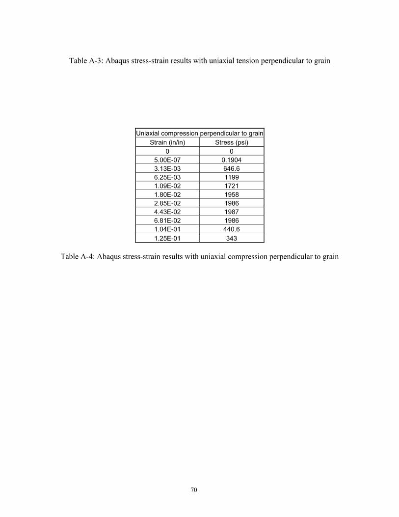
70

Table A-3: Abaqus stress-strain results with uniaxial tension perpendicular to grain

Uniaxial compression perpendicular to grainStrain (in/in) Stress (psi)

0 0 5.00E-07 0.1904 3.13E-03 646.6 6.25E-03 1199 1.09E-02 1721 1.80E-02 1958 2.85E-02 1986 4.43E-02 1987 6.81E-02 1986 1.04E-01 440.6 1.25E-01 343

Table A-4: Abaqus stress-strain results with uniaxial compression perpendicular to grain

71

Damage Var i abl e( Tensi on | | Grai n)

*7*6*5*4

*3*1*20. 0000

0. 5000

1. 0000

1. 5000

0. 0004 0. 0054 0. 0104 0. 0154

St rai nD

amag

e Va

riabl

e

Notation:

*1. Damage variable =0.00. The initial constitutive matrix.

×××××

=4

44

45

1049.7000105.83101.70-0101.70-104.45

C .

*2. Damage variable =0.063. The constitutive matrix

×××××

=4

4

45

1002.70001083.5101.74-0101.74-0191.3

C .

*3. Damage variable =0.224. The constitutive matrix

×××××

=4

44

4

1081.50001083.5101.84-0101.84-1052.71

C .

*4. Damage variable =0.514. The constitutive matrix

×××−×−×

=4

45

55

1065.30001082.51097.101097.1101.11

C .

*5. Damage variable =0.813. The constitutive matrix

×××−×−×

=4

44

44

1040.1000105.821004.201004.21026.2

C .

*6. Damage variable =0.964. The constitutive matrix

×××−×−×

=2

44

43

1001.2000105.821006.201006.21082.7

C .

*7. Damage variable =1.000. The constitutive matrix

×××−×−×

=2

44

43

1001.2000105.821006.201006.21026.7

C .

Table A-9: The constitutive matrix corresponding to different damage levels

(Uniaxial Tension Parallel to Grain)

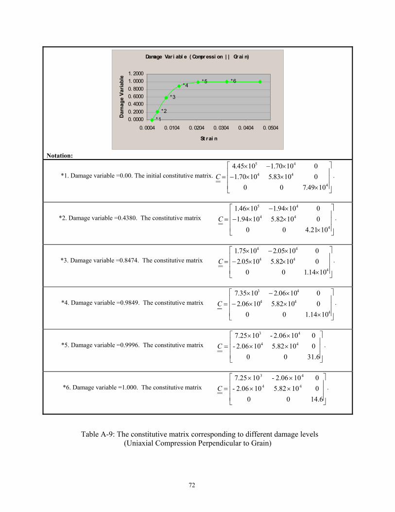
72

Damage Var i abl e ( Compressi on | | Grai n)

*6*5*4

*3

*2*10. 0000

0. 20000. 40000. 60000. 80001. 00001. 2000

0. 0004 0. 0104 0. 0204 0. 0304 0. 0404 0. 0504

St rai n

Dam

age

Varia

ble

Notation:

*1. Damage variable =0.00. The initial constitutive matrix.

×××−×−×

=4

44

45

1049.70001083.51070.101070.11045.4

C .

*2. Damage variable =0.4380. The constitutive matrix

×××−×−×

=4

44

45

104.21000105.821094.101094.11046.1

C .

*3. Damage variable =0.8474. The constitutive matrix

×××−×−×

=4

44

44

1014.1000105.821005.201005.21075.1

C .

*4. Damage variable =0.9849. The constitutive matrix

×××−×−×

=4

44

43

1014.10001082.51006.201006.21035.7

C .

*5. Damage variable =0.9996. The constitutive matrix

××××

=6.3100

010.825102.06-0102.06-10.257

44

43

C .

*6. Damage variable =1.000. The constitutive matrix

××××

=6.1400

010.825102.06-0102.06-10.257

44

43

C .

Table A-9: The constitutive matrix corresponding to different damage levels (Uniaxial Compression Perpendicular to Grain)

73

APPENDIX B

ABAQUS User Subroutine For the HDPE Material Model

74

HDPE MATERIAL MODEL

MACRO FLOW CHART OF THE UMAT SUBROUTINE

Figure B-1: Macro flow chart of the UMAT subroutine for the HDPE material model

INPUT MATERAL CONSTANTS

SAVE RESULTS INTO STATE VARIABLES

INITIALIZE THE CONSTITUTIVE

MATRIX

COMPUTE EIGENVALUES

EIGENVECTORS

COMPUTE DAMAGE

EVOLUTION

SAVE D INTO STATE

VARIABLES

GENERATE NEW CONSTITUTIVE

MATRIX

OUTPUT CURRENT

STRESS AND STRAIN

ABAQUS CORE

PROGRAMS

COMPUTE

EIGENSRAINS

COMPUTE VOLUMETRIC

STRAIN

IF INCREMENT

No.1

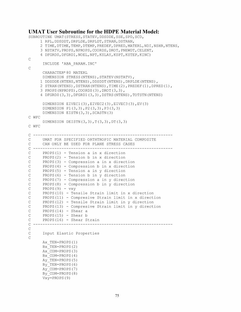
75

UMAT User Subroutine for the HDPE Material Model: SUBROUTINE UMAT(STRESS,STATEV,DDSDDE,SSE,SPD,SCD, 1 RPL,DDSDDT,DRPLDE,DRPLDT,STRAN,DSTRAN, 2 TIME,DTIME,TEMP,DTEMP,PREDEF,DPRED,MATERL,NDI,NSHR,NTENS, 3 NSTATV,PROPS,NPROPS,COORDS,DROT,PNEWDT,CELENT, 4 DFGRD0,DFGRD1,NOEL,NPT,KSLAY,KSPT,KSTEP,KINC) C INCLUDE 'ABA_PARAM.INC' C CHARACTER*80 MATERL DIMENSION STRESS(NTENS),STATEV(NSTATV), 1 DDSDDE(NTENS,NTENS),DDSDDT(NTENS),DRPLDE(NTENS), 2 STRAN(NTENS),DSTRAN(NTENS),TIME(2),PREDEF(1),DPRED(1), 3 PROPS(NPROPS),COORDS(3),DROT(3,3), 4 DFGRD0(3,3),DFGRD1(3,3),DSTRS(NTENS),TOTSTN(NTENS) DIMENSION EIVEC1(3),EIVEC2(3),EIVEC3(3),EV(3) DIMENSION P1(3,3),P2(3,3),P3(3,3) DIMENSION EISTN(3,3),SCASTN(3) C WFC DIMENSION DEISTN(3,3),T(3,3),DT(3,3) C WFC C ----------------------------------------------------------- C UMAT FOR SPECIFIED ORTHTROPIC MATERIAL COMPOSITE C CAN ONLY BE USED FOR PLANE STRESS CASES C ----------------------------------------------------------- C PROPS(1) - Tension a in x direction C PROPS(2) - Tension b in x direction C PROPS(3) - Compression a in x direction C PROPS(4) - Compression b in x direction C PROPS(5) - Tension a in y direction C PROPS(6) - Tension b in y direction C PROPS(7) - Compression a in y direction C PROPS(8) - Compression b in y direction C PROPS(9) - vxy C PROPS(10) - Tensile Strain limit in x direction C PROPS(11) - Compresive Strain limit in x direction C PROPS(12) - Tensile Strain limit in y direction C PROPS(13) - Compresive Strain limit in y direction C PROPS(14) - Shear a C PROPS(15) - Shear b C PROPS(16) - Shear Strain C ----------------------------------------------------------- C C Input Elastic Properties C Ax_TEN=PROPS(1) Bx_TEN=PROPS(2) Ax_COM=PROPS(3) Bx_COM=PROPS(4) Ay_TEN=PROPS(5) By_TEN=PROPS(6) Ay_COM=PROPS(7) By_COM=PROPS(8) Vxy=PROPS(9)

76

a3=PROPS(14) b3=PROPS(15) C C Damage Properties C STNLxt=PROPS(10) STNLxc=PROPS(11) STNLyt=PROPS(12) STNLyc=PROPS(13) D1=STATEV(1) D2=STATEV(2) D3=STATEV(3) d1wfc=statev(25) d2wfc=statev(26) d3wfc=statev(27) stnlxtf=1.5*stnlxt stnlxcf=1.5*stnlxc stnlytf=1.2*stnlyt stnlycf=1.5*stnlyc dd1wfc=0. dd2wfc=0. dd3wfc=0. D1NEW=D1 D2NEW=D2 D3NEW=D3 DD1=0. DD2=0. DD3=0. C C Define Elastic Properties According to Strain State C DO II=1,NTENS TOTSTN(II)=STRAN(II)+DSTRAN(II) END DO STNx=STATEV(4) STNy=STATEV(5) STNxy=STATEV(6) DSTNx=DSTRAN(1) DSTNy=DSTRAN(2) DSTNxy=DSTRAN(3) C STRx=STATEV(19) C STRy=STATEV(20) C STRxy=STATEV(21) VMSTN1=STATEV(14) VMSTN2=STATEV(15) STATEV(7)=STATEV(7)+1.0 IF (STATEV(7).EQ.1.0) THEN a1=(Ax_COM+Ax_TEN)/2.0 a2=(Ay_COM+Ay_TEN)/2.0 Ex=(Ax_COM*Bx_COM+Ax_TEN*Bx_TEN)/2.0 Ey=(Ay_COM*By_COM+Ay_TEN*By_TEN)/2.0 ELSE IF(STATEV(7).EQ.2.0) THEN

77

IF (VMSTN1.GT.1.e-8) THEN a1=Ax_TEN Ex=Ax_TEN*Bx_TEN STNL1=STNLxt stnl1f=stnlxtf STATEV(8)=Ex STATEV(9)=a1 STATEV(10)=STNL1 statev(28)=stnl1f C ELSE a1=Ax_COM Ex=Ax_COM*Bx_COM STNL1=STNLxc stnl1f=stnlxcf STATEV(8)=Ex STATEV(9)=a1 STATEV(10)=STNL1 statev(28)=stnl1f ENDIF C IF (VMSTN2.GT.1.e-8) THEN a2=Ay_TEN Ey=Ay_TEN*By_TEN STNL2=STNLyt stnl2f=stnlytf STATEV(11)=Ey STATEV(12)=a2 STATEV(13)=STNL2 statev(29)=stnl2f ELSE a2=Ay_COM Ey=Ay_COM*By_COM STNL2=STNLyc stnl2f=stnlycf STATEV(11)=Ey STATEV(12)=a2 STATEV(13)=STNL2 statev(29)=stnl2f ENDIF ELSE Ex=STATEV(8) a1=STATEV(9) STNL1=STATEV(10) stnl1f=statev(28) Ey=STATEV(11) a2=STATEV(12) STNL2=STATEV(13) stnl2f=statev(29) ENDIF Gxy=a3*b3 Vyx=Ey*Vxy/Ex

78

C ----------------------------------------------------------- C CACULATE EIGENVALUES AND EIGENVECTORS C ----------------------------------------------------------- TERM1=1.0/(1.0-Vxy*Vyx) C11=Ex*TERM1 C12=Vxy*Ex*TERM1 C21=Vyx*Ey*TERM1 C22=Ey*TERM1 C66=Gxy EV(3)=2*C66 EV(1)=(C22+C11+SQRT(C22**2+C11**2-2*C11*C22+4*C12*C21))/2.0 EV(2)=(C22+C11-SQRT(C22**2+C11**2-2*C11*C22+4*C12*C21))/2.0 TEMP0=-C12/(C11-EV(1)) TEMP1=SQRT((-C12/(C11-EV(1)))**2+1.0) TEMP2=-C12/(C11-EV(2)) TEMP3=SQRT((-C12/(C11-EV(2)))**2+1.0) EIVEC1(1)=TEMP0/TEMP1 EIVEC1(2)=1./TEMP1 EIVEC1(3)=0. EIVEC2(1)=TEMP2/TEMP3 EIVEC2(2)=1./TEMP3 EIVEC2(3)=0. EIVEC3(1)=0. EIVEC3(2)=0. EIVEC3(3)=1. C------------------------------------------------ C DAMAGE EVOLUTION C SCASTN(I)------SCALAR STRAIN C DDx--------DAMAGE INCREMENT FOR MODE X C------------------------------------------------ DO I=1,3 EISTN(1,I)=0. EISTN(2,I)=0. EISTN(3,I)=0. DEISTN(1,I)=0. DEISTN(2,I)=0. DEISTN(3,I)=0. T(1,I)=0. T(2,I)=0. T(3,I)=0. SCASTN(I)=0. END DO DO I=1,3 DO J=1,3 P1(I,J)=0.

79

P2(I,J)=0. P3(I,J)=0. END DO END DO DO I=1,3 DO J=1,3 P1(I,J)=P1(I,J)+EIVEC1(I)*EIVEC1(J) P2(I,J)=P2(I,J)+EIVEC2(I)*EIVEC2(J) P3(I,J)=P3(I,J)+EIVEC3(I)*EIVEC3(J) END DO END DO DO I=1,3 EISTN(1,I)=EISTN(1,I)+P1(I,1)*STNx + +P1(I,2)*STNy+P1(I,3)*STNxy*1.414213562 EISTN(2,I)=EISTN(2,I)+P2(I,1)*STNx + +P2(I,2)*STNy+P2(I,3)*STNxy*1.414213562 EISTN(3,I)=EISTN(3,I)+P3(I,1)*STNx + +P3(I,2)*STNy+P3(I,3)*STNxy*1.414213562 DEISTN(1,I)=DEISTN(1,I)+P1(I,1)*DSTNx + +P1(I,2)*DSTNy+P1(I,3)*DSTNxy*1.414213562 DEISTN(2,I)=DEISTN(2,I)+P2(I,1)*DSTNx + +P2(I,2)*DSTNy+P2(I,3)*DSTNxy*1.414213562 DEISTN(3,I)=DEISTN(3,I)+P3(I,1)*DSTNx + +P3(I,2)*DSTNy+P3(I,3)*DSTNxy*1.414213562 END DO T(1,1)=STATEV(16) T(1,2)=STATEV(17) T(1,3)=STATEV(18) T(2,1)=STATEV(19) T(2,2)=STATEV(20) T(2,3)=STATEV(21) T(3,1)=STATEV(22) T(3,2)=STATEV(23) T(3,3)=STATEV(24) C WRITE(6,'(3E12.5)')STNx, STNy, STNxy C write (6,*) 'stress ',stress(1),stress(2),stress(3) C write (6,*) 'T, 1', t(1,1),t(2,1),t(3,1) C write (6,*) 'T, 2',t(1,2),t(2,2),t(3,2) C write (6,*) 'T, 3',t(1,3),t(2,3),t(3,3) VMSTN1=EISTN(1,1)+EISTN(1,2)+EISTN(1,3) VMSTN2=EISTN(2,1)+EISTN(2,2)+EISTN(2,3) dvmstn1=deistn(1,1)+deistn(1,2)+deistn(1,3) dvmstn2=deistn(2,1)+deistn(2,2)+deistn(2,3) IF(VMSTN1.GT.-1.E-8) THEN STATEV(14)=1.0 ELSE STATEV(14)=0. ENDIF IF(VMSTN2.GT.-1.E-8) THEN STATEV(15)=1.0 ELSE

80

STATEV(15)=0. ENDIF DO I=1,3 SCASTN(1)=SCASTN(1)+EISTN(1,I)*EISTN(1,I) SCASTN(2)=SCASTN(2)+EISTN(2,I)*EISTN(2,I) SCASTN(3)=SCASTN(3)+EISTN(3,I)*EISTN(3,I) END DO DO I=1,3 SCASTN(I)=SQRT(SCASTN(I)) END DO IF (SCASTN(1).LE.1E-8.AND.SCASTN(2).LE.1E-8) THEN SCASTN(1)=SCASTN(3)*1.0/2. SCASTN(2)=SCASTN(3)*1.0/2. STATEV(14)=1.0 STATEV(15)=0. ELSE SCASTN(1)=SCASTN(1)+SCASTN(3)*1.0/2. SCASTN(2)=SCASTN(2)+SCASTN(3)*1.0/2. END IF D1NEW=1-(1/COSH(EV(1)*SCASTN(1)/a1))**2 IF (D1NEW.GT.1.) THEN D1NEW=1.0 ENDIF DD1=D1NEW-D1 STATEV(1)=D1NEW IF (DD1.LT.0.) DD1=0. if (abs(scastn(1)).gt.stnl1) then d1wfcnew=(abs(scastn(1))-stnl1)/(stnl1f-stnl1) if (d1wfcnew.gt.1.) d1wfcnew=1. dd1wfc=d1wfcnew-d1wfc statev(25)=d1wfcnew endif if (abs(scastn(2)).gt.stnl2) then d2wfcnew=(abs(scastn(2))-stnl2)/(stnl2f-stnl2) if (d2wfcnew.gt.1.) d2wfcnew=1. dd2wfc=d2wfcnew-d2wfc statev(26)=d2wfcnew endif D2NEW=1-(1/COSH(EV(2)*SCASTN(2)/a2))**2 IF (D2NEW.GT.1.) THEN D2NEW=1.0 ENDIF DD2=D2NEW-D2 STATEV(2)=D2NEW IF (DD2.LT.0.) DD2=0.

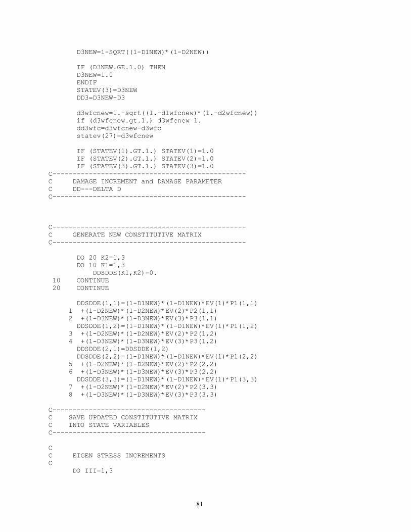
81

D3NEW=1-SQRT((1-D1NEW)*(1-D2NEW)) IF (D3NEW.GE.1.0) THEN D3NEW=1.0 ENDIF STATEV(3)=D3NEW DD3=D3NEW-D3 d3wfcnew=1.-sqrt((1.-d1wfcnew)*(1.-d2wfcnew)) if (d3wfcnew.gt.1.) d3wfcnew=1. dd3wfc=d3wfcnew-d3wfc statev(27)=d3wfcnew IF (STATEV(1).GT.1.) STATEV(1)=1.0 IF (STATEV(2).GT.1.) STATEV(2)=1.0 IF (STATEV(3).GT.1.) STATEV(3)=1.0 C------------------------------------------------ C DAMAGE INCREMENT and DAMAGE PARAMETER C DD---DELTA D C------------------------------------------------ C------------------------------------------------ C GENERATE NEW CONSTITUTIVE MATRIX C------------------------------------------------ DO 20 K2=1,3 DO 10 K1=1,3 DDSDDE(K1,K2)=0. 10 CONTINUE 20 CONTINUE DDSDDE(1,1)=(1-D1NEW)*(1-D1NEW)*EV(1)*P1(1,1) 1 +(1-D2NEW)*(1-D2NEW)*EV(2)*P2(1,1) 2 +(1-D3NEW)*(1-D3NEW)*EV(3)*P3(1,1) DDSDDE(1,2)=(1-D1NEW)*(1-D1NEW)*EV(1)*P1(1,2) 3 +(1-D2NEW)*(1-D2NEW)*EV(2)*P2(1,2) 4 +(1-D3NEW)*(1-D3NEW)*EV(3)*P3(1,2) DDSDDE(2,1)=DDSDDE(1,2) DDSDDE(2,2)=(1-D1NEW)*(1-D1NEW)*EV(1)*P1(2,2) 5 +(1-D2NEW)*(1-D2NEW)*EV(2)*P2(2,2) 6 +(1-D3NEW)*(1-D3NEW)*EV(3)*P3(2,2) DDSDDE(3,3)=(1-D1NEW)*(1-D1NEW)*EV(1)*P1(3,3) 7 +(1-D2NEW)*(1-D2NEW)*EV(2)*P2(3,3) 8 +(1-D3NEW)*(1-D3NEW)*EV(3)*P3(3,3) C-------------------------------------- C SAVE UPDATED CONSTITUTIVE MATRIX C INTO STATE VARIABLES C-------------------------------------- C C EIGEN STRESS INCREMENTS C DO III=1,3

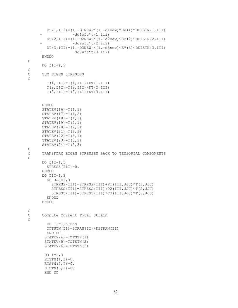
82

DT(1,III)=(1.-D1NEW)*(1.-d1new)*EV(1)*DEISTN(1,III) + -dd1wfc*t(1,iii) DT(2,III)=(1.-D2NEW)*(1.-d2new)*EV(2)*DEISTN(2,III) + -dd2wfc*t(2,iii) DT(3,III)=(1.-D3NEW)*(1.-d3new)*EV(3)*DEISTN(3,III) + -dd3wfc*t(3,iii) ENDDO C DO III=1,3 C C SUM EIGEN STRESSES C T(1,III)=T(1,III)+DT(1,III) T(2,III)=T(2,III)+DT(2,III) T(3,III)=T(3,III)+DT(3,III) ENDDO STATEV(16)=T(1,1) STATEV(17)=T(1,2) STATEV(18)=T(1,3) STATEV(19)=T(2,1) STATEV(20)=T(2,2) STATEV(21)=T(2,3) STATEV(22)=T(3,1) STATEV(23)=T(3,2) STATEV(24)=T(3,3) C C TRANSFORM EIGEN STRESSES BACK TO TENSORIAL COMPONENTS C DO III=1,3 STRESS(III)=0. ENDDO DO III=1,3 DO JJJ=1,3 STRESS(III)=STRESS(III)+P1(III,JJJ)*T(1,JJJ) STRESS(III)=STRESS(III)+P2(III,JJJ)*T(2,JJJ) STRESS(III)=STRESS(III)+P3(III,JJJ)*T(3,JJJ) ENDDO ENDDO C C Compute Current Total Strain C DO II=1,NTENS TOTSTN(II)=STRAN(II)+DSTRAN(II) END DO STATEV(4)=TOTSTN(1) STATEV(5)=TOTSTN(2) STATEV(6)=TOTSTN(3) DO I=1,3 EISTN(1,I)=0. EISTN(2,I)=0. EISTN(3,I)=0. END DO

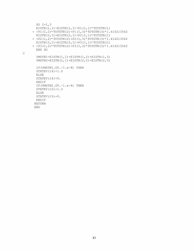
83

DO I=1,3 EISTN(1,I)=EISTN(1,I)+P1(I,1)*TOTSTN(1) + +P1(I,2)*TOTSTN(2)+P1(I,3)*TOTSTN(3)*1.414213562 EISTN(2,I)=EISTN(2,I)+P2(I,1)*TOTSTN(1) + +P2(I,2)*TOTSTN(2)+P2(I,3)*TOTSTN(3)*1.414213562 EISTN(3,I)=EISTN(3,I)+P3(I,1)*TOTSTN(1) + +P3(I,2)*TOTSTN(2)+P3(I,3)*TOTSTN(3)*1.414213562 END DO C VMSTN1=EISTN(1,1)+EISTN(1,2)+EISTN(1,3) VMSTN2=EISTN(2,1)+EISTN(2,2)+EISTN(2,3) IF(VMSTN1.GT.-1.e-8) THEN STATEV(14)=1.0 ELSE STATEV(14)=0. ENDIF IF(VMSTN2.GT.-1.e-8) THEN STATEV(15)=1.0 ELSE STATEV(15)=0. ENDIF RETURN END

84

APPENDIX C

ABAQUS Input and Output File for the HDPE Material Model

85

Execution Procedures of Input File: *Define nodes *Define type of element and element group *Define element section *Define orientation *Define material Input material constants and properties Implement user subroutine *Specify the number of state variables *Definition of step *Indicate type of analysis *Define an amplitude curve *Define boundary conditions *Set time incrementation control parameters *Output results

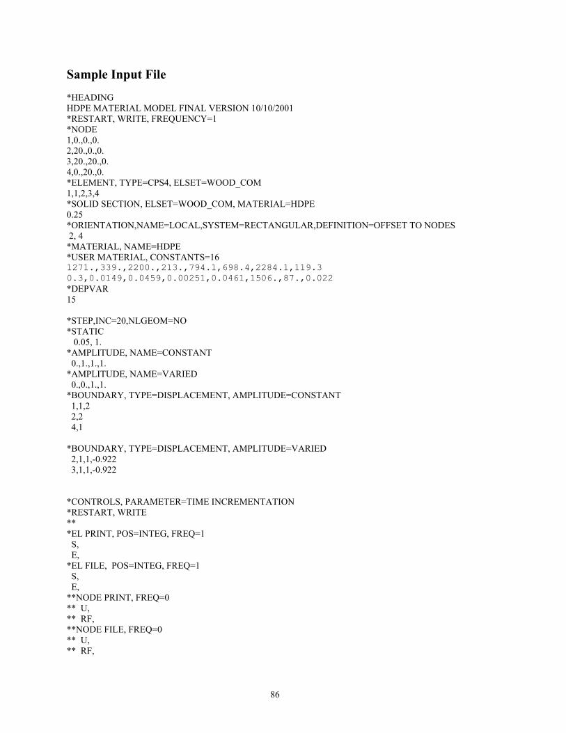
86

Sample Input File *HEADING HDPE MATERIAL MODEL FINAL VERSION 10/10/2001 *RESTART, WRITE, FREQUENCY=1 *NODE 1,0.,0.,0. 2,20.,0.,0. 3,20.,20.,0. 4,0.,20.,0. *ELEMENT, TYPE=CPS4, ELSET=WOOD_COM 1,1,2,3,4 *SOLID SECTION, ELSET=WOOD_COM, MATERIAL=HDPE 0.25 *ORIENTATION,NAME=LOCAL,SYSTEM=RECTANGULAR,DEFINITION=OFFSET TO NODES 2, 4 *MATERIAL, NAME=HDPE *USER MATERIAL, CONSTANTS=16 1271.,339.,2200.,213.,794.1,698.4,2284.1,119.3 0.3,0.0149,0.0459,0.00251,0.0461,1506.,87.,0.022 *DEPVAR 15 *STEP,INC=20,NLGEOM=NO *STATIC 0.05, 1. *AMPLITUDE, NAME=CONSTANT 0.,1.,1.,1. *AMPLITUDE, NAME=VARIED 0.,0.,1.,1. *BOUNDARY, TYPE=DISPLACEMENT, AMPLITUDE=CONSTANT 1,1,2 2,2 4,1 *BOUNDARY, TYPE=DISPLACEMENT, AMPLITUDE=VARIED 2,1,1,-0.922 3,1,1,-0.922 *CONTROLS, PARAMETER=TIME INCREMENTATION *RESTART, WRITE ** *EL PRINT, POS=INTEG, FREQ=1 S, E, *EL FILE, POS=INTEG, FREQ=1 S, E, **NODE PRINT, FREQ=0 ** U, ** RF, **NODE FILE, FREQ=0 ** U, ** RF,

87

** *EL PRINT, POS=NODES, FREQ=0 ** *EL FILE, POS=NODES, FREQ=0 ** *EL PRINT, POS=CENTR, FREQ=1 S, E, *EL FILE, POS=CENTR, FREQ=1 S, E, *EL PRINT, POS=AVERAGE, FREQ=1 S, E, *EL FILE, POS=AVERAGE, FREQ=1 S, E, *MODAL PRINT, FREQ=0 ** *MODAL FILE, FREQ=0 ** *ENERGY PRINT, FREQ=0 ** *ENERGY FILE, FREQ=0 ** *PRINT, FREQ=1 ** *END STEP

88

References

1. American Society of Testing Materials, (1998) Standard Test Method for Shear Properties of Composite Materials by the V-notched Beam Method, ASTM D5379.

2. Arramon, Y. P., Mehrabadi, M. M., Martin D. W., Cowin, S. C., (2000) A Multidimentional Anistropic Strength Criterion Based on Kelvin Modes, International Journal of Solids and Structures, Pergamon Press, 37, 2915-2935.

3. Biegler, M.W., Mehrabadi, M. M., (1995). An energy-based constitutive model for anisotropic solids subject to damage. Mechanics of Materials, Elsevier, 19, 151-164.

4. Caiazzo, A.A., Costanzo, F., (2000) On the constitutive relations of materials with

evolving microstructure due to microcracking, International Journal of Solids and Structures, Pergamon Press, 37, 3375-3398.

5. Chow, C.L., Lu, T.J., (1989) On evolution laws of anisotropic damage, Engineering

Fracture Mechanics, Pergamon Press, 34, 679-701.

6. Cofer, W. F., Mclean, D. I., Paynter, M. E., Wang, H., (1998) The Development and Verification of Finite Element Models to Optimize the design of Wale/Chock Structural Sections, Prepared for Office of Naval Research under Contract N00014-97-C-0395, 1998 Yearly Report, Washington State University, Pullman, WA.

7. Cofer, W. F., Yang, W., (1999) The Development and Verification of Finite Element

Models to Optimize the design of Wale/Chock Structural Sections, Prepared for Office of Naval Research under Contract N00014-97-C-0395, 1999 Yearly Report, Washington State University, Pullman, WA.

8. Coleman, B.D., Gurtin, M.E., (1967) Thermodynamics with Internal State Variables,

Journal of Chemical Physics, 47, 597-613.

9. Coleman, B.D., Noll, W., (1963) The Thermodynamics of Elastic Materials with Heat Conduction and Viscosity, Archive for Rational Mechanics and Analysis, 18, 245-261.

10. Cowin S. C., Mehrabadi, M. M., (1992) The Structure of The Linear Anisotropic

Elastic Symmetries, J. Mech. Phys. Solids, 40.7, 1459-1471.

11. Germain, P., Nguyen, Q.S., Suquet, P.M., (1983) Continuum Thermodynamics, Journal of Applied Mechanics, 50, 1010-1020.

12. Haiar, K. J., (2000) Performance and Design of Prototype Wood-Plastic Composite

Sections, Thesis for partial fulfillment of the degree of Master of Science, Washington State University, Pullman, WA.

89

13. Lemaitre, J., (1983) A Continuous Damage Mechanics Model for Ductile Fracture, J. of Engineering Materials and Technology, 107, 83-89.

14. Lockyear, S. A., (1999) Mechanical Analysis of Transversely Loaded Wood/Plastic

sections, Thesis for partial fulfillment of the degree of Master of Science, Washington State University, Pullman, WA.

15. Matzenmiller, A., Lubliner, J., Taylor, R.L., (1995) A Constitutive Model for Anisotropic Damage in Fiber-composites, Mechanics of Materials, Elsevier Science, 20, 125-152.

16. Mehrabadi, M. M., Cowin S. C., (1990) Eigentensors of Linear Anisotropic elastic materials, Q. J. Mech. Appl. Math., 43.1, 15-41

17. Schreyer, H.L., Zuo, Q.H., (1995) Anisotropic Yield Surfaces Based on Elastic Projection Operators, J Appl. Mech., 62, 780-785.

18. Zhu Y. and Cescotto S., (1995) A Fully Coupled Elastic-visco-plastic Damage Theory

for Anisotropic Materials, International Jounal of Solids and Structures, 32,11, 1607-1641.