Hazard rate models for early warranty issue detection

Wayne State University

Wayne State University Dissertations

1-1-2011

Hazard rate models for early warranty issuedetection using upstream supply chain informationChongwen ZhouWayne State University,

Follow this and additional works at: http://digitalcommons.wayne.edu/oa_dissertations

Part of the Industrial Engineering Commons

This Open Access Dissertation is brought to you for free and open access by DigitalCommons@WayneState. It has been accepted for inclusion inWayne State University Dissertations by an authorized administrator of DigitalCommons@WayneState.

Recommended CitationZhou, Chongwen, "Hazard rate models for early warranty issue detection using upstream supply chain information" (2011). WayneState University Dissertations. Paper 404.

http://digitalcommons.wayne.edu/?utm_source=digitalcommons.wayne.edu%2Foa_dissertations%2F404&utm_medium=PDF&utm_campaign=PDFCoverPages

http://digitalcommons.wayne.edu/?utm_source=digitalcommons.wayne.edu%2Foa_dissertations%2F404&utm_medium=PDF&utm_campaign=PDFCoverPages

http://digitalcommons.wayne.edu/oa_dissertations?utm_source=digitalcommons.wayne.edu%2Foa_dissertations%2F404&utm_medium=PDF&utm_campaign=PDFCoverPages

http://digitalcommons.wayne.edu/oa_dissertations?utm_source=digitalcommons.wayne.edu%2Foa_dissertations%2F404&utm_medium=PDF&utm_campaign=PDFCoverPages

http://network.bepress.com/hgg/discipline/307?utm_source=digitalcommons.wayne.edu%2Foa_dissertations%2F404&utm_medium=PDF&utm_campaign=PDFCoverPages

http://digitalcommons.wayne.edu/oa_dissertations/404?utm_source=digitalcommons.wayne.edu%2Foa_dissertations%2F404&utm_medium=PDF&utm_campaign=PDFCoverPages

HAZARD RATE MODELS FOR EARLY WARRANTY ISSUE DETECTION USING UPSTREAM SUPPLY CHAIN INFORMATION

by

CHONGWEN ZHOU

DISSERTATION

Submitted to the Graduate School

of Wayne State University,

Detroit, Michigan

in partial fulfillment of the requirements

for the degree of

DOCTOR OF PHILOSOPHY

2011

MAJOR:INDUSTRIAL ENGINEERING

Approved by:

Advisor Date

ii

DEDICATION

Dedicated to my wife and daughter Wei and Qijia

iii

ACKNOWLEDGMENTS

I owe my deepest gratitude to my advisor Dr. Ratna Babu Chinnam for his

understanding, patience, encouragement and guidance. Without his continued support

and interest, it would have been next to impossible for me, as a part time PhD student

with a full time job, to complete this dissertation.

I also wish to express my sincere appreciation to my co-advisor Dr Alexander

Korostelev for his technical advice in statistics.

I am also very thankful to Dr. Kai Yang and Dr. Alper E. Murat for their support and

understanding.

Finally I would like to thank my company Faurecia and my manager Brian Kormendy

for providing an excellent environment to work, experience and data source to motivate

and enrich my PhD research. Anyway, PhD research should come from real life and

work for better real life.

iv

TABLE OF CONTENTS

Dedication ....................................................................................................................... ii

Acknowledgments ........................................................................................................... iii

List of Figures ................................................................................................................. vii

List of Tables ................................................................................................................... x

CHAPTER 1 Introduction ............................................................................................ 1

1.1 Research Motivation ......................................................................................... 2

1.2 Research Objectives and Scope ....................................................................... 4

CHAPTER 2 Hazard Rate Models for Early Warranty Issue Detection Using

Upstream Supply Chain Information ................................................................................ 6

2.1 Introduction ....................................................................................................... 6

2.2 Literature Review .............................................................................................. 6

2.3 Upstream Data Sources for Early Warranty Detection .................................... 10

2.3.1 OEM Warranty Data Sources/Structure ................................................... 11

2.3.2 Supplier Network Warranty Data Sources/Structure ................................ 12

2.4 Correlating Upstream Quality/Testing Data to Warranty Claims ..................... 15

2.4.1 Hazard Rate Models ................................................................................ 18

2.4.2 Proportional Hazard (PH) Model .............................................................. 18

2.4.3 Parametric vs. Semi-Parametric PH Models ............................................ 19

2.4.4 Estimating PH Model Parameters from Past/Current Warranty Datasets 20

2.4.5 Selection of Covariates ............................................................................ 22

2.4.6 PH Model Development ........................................................................... 24

2.5 Early Warranty Detection Scheme .................................................................. 25

v

2.5.1 Notation and Assumptions ....................................................................... 25

2.5.2 Binomial Distribution Model for Monitoring Warranty Claims ................... 27

2.5.3 Hypothesis Test ....................................................................................... 28

2.5.4 Allocation of False Alarm Probability and Power for Detection ................ 31

2.6 Case Study ..................................................................................................... 32

2.6.1 Data ......................................................................................................... 32

2.6.2 Covariates ................................................................................................ 34

2.6.3 Model Estimation ..................................................................................... 35

2.6.4 Model Validation ...................................................................................... 39

2.7 Conclusion ...................................................................................................... 47

CHAPTER 3 Bayesian Approach to Hazard Rate Models for Early Warranty Issues

Detection ............................................................................................................. 49

3.1 Introduction ..................................................................................................... 49

3.2 Bayesian Approach to Encapsulate Upstream Supply Chain Information ....... 51

3.3 Statistical Framework to Obtain Posterior Distribution of Hazard Rate Model 54

3.3.1 Large Sample Size Bayesian Analysis .................................................... 59

3.3.2 Monte Carlo Markov Chain (MCMC) Bayesian Analysis .......................... 63

3.4 Constructing Prior for ................................................................................ 68

3.5 Case Study ..................................................................................................... 71

3.5.1 Data ......................................................................................................... 72

3.5.2 Retrospective Estimation of Impact of New Design on Hazard Rate ....... 74

3.5.3 Estimation of Baseline Hazard ................................................................. 76

3.5.4 Eliciting Prior Distribution of For the New Design ............................ 77

vi

3.5.5 Estimating Posterior Distribution of or for New Design ................ 81

3.5.6 Hypothesis Testing of or ........................................................... 86

3.5.7 Performance Review: Large Sample Size vs. MCMC Bayesian Analysis 92

3.6 Conclusion ...................................................................................................... 92

CHAPTER 4 Summary and Conclusions .................................................................. 94

4.1 Summary and Research Contribution ............................................................. 94

4.2 Limitations and Recommendations for Future Research ................................ 96

References .................................................................................................................... 98

Abstract ....................................................................................................................... 107

Autobiographical Statement ........................................................................................ 108

vii

LIST OF FIGURES

Figure 1: Data sources for modeling warranty issues from supply network upstream to customer downstream; Adopted from (Majeske, 2007; Murthy, 2010). ........... 3

Figure 2: Warranty claims, covariates and vehicle volumes growth diagram stratified by production. .................................................................................................... 30

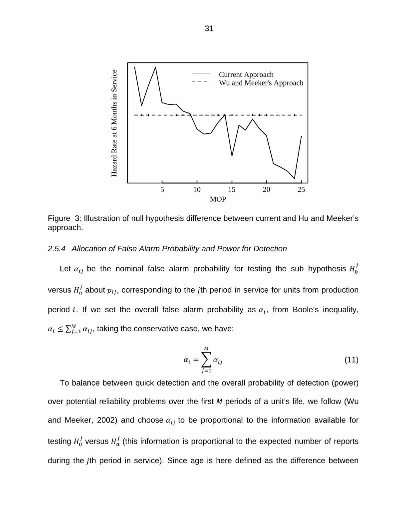
Figure 3: Illustration of null hypothesis difference between current and Hu and Meeker’s approach. ...................................................................................................... 31

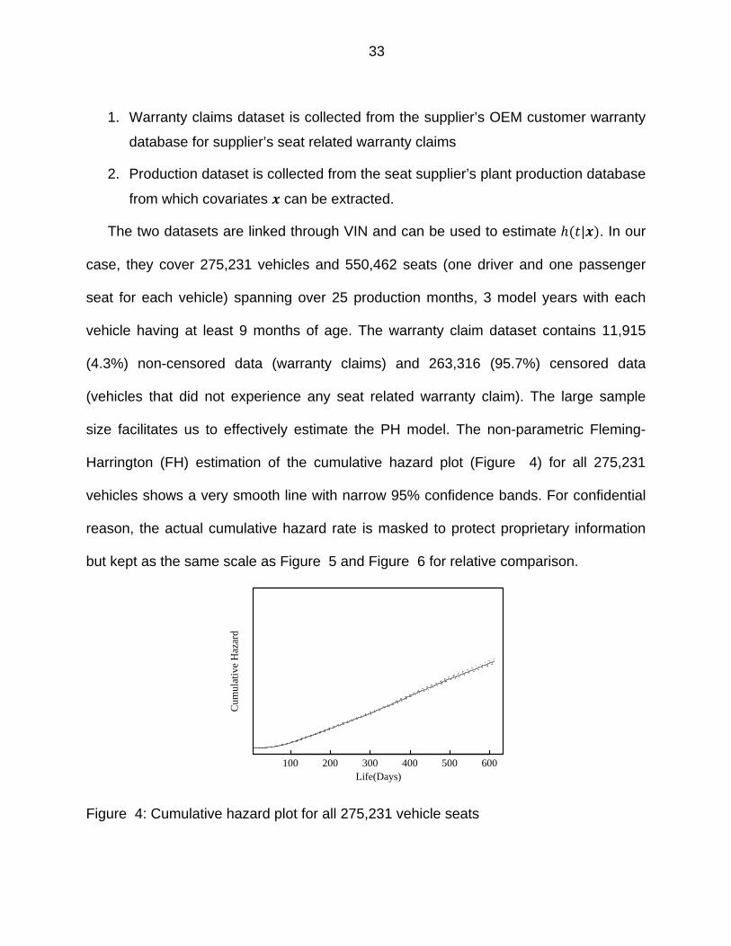
Figure 4: Cumulative hazard plot for all 275,231 vehicle seats .................................... 33

Figure 5: Cumulative hazard plot stratified by MOPs .................................................... 36

Figure 6: Cumulative hazard plot stratified by SeatType ............................................... 37

Figure 7: Plots of scaled Schoenfield residuals against transformed time for the different covariates. ....................................................................................... 40

Figure 8: Plots influence by observation number for the different covariates. .............. 40

Figure 9: Martingale-residual plots for the different covariates. .................................... 41

Figure 10: Hypothesis test results comparison between the proposed PH model (a) and Wu & Meeker (2002) (b) for warranty claims from vehicles during first month in service (prediction limits and actual claims). ............................................. 43

Figure 11: Hypothesis test results comparison between the proposed PH model (a) and Wu & Meeker (2002) (b) for warranty claims from vehicles during the second month in service. ........................................................................................... 43

Figure 12: Hypothesis test results comparison between the proposed PH model (a) and Wu & Meeker (2002) (b) for warranty claims from vehicles during the third month in service. ........................................................................................... 44

Figure 13: Hypothesis test results comparison between the proposed PH model (a) and Wu & Meeker (2002) (b) for warranty claims from vehicles during the fourth month in service. ........................................................................................... 44

Figure 14: Hypothesis test results comparison between the proposed PH model (a) and Wu & Meeker (2002) (b) for warranty claims from vehicles during the fifth month in service. ........................................................................................... 45

viii

Figure 15: Hypothesis test results comparison between the proposed PH model (a) and Wu & Meeker (2002) (b) for warranty claims from vehicles during the sixth month in service. ........................................................................................... 45

Figure 16: Hypothesis test results comparison between the proposed PH model (a) and Wu & Meeker (2002) (b) for warranty claims from vehicles during the seventh month in service. ........................................................................................... 46

Figure 17: Hypothesis test results comparison between the proposed PH model (a) and Wu & Meeker (2002) (b) for warranty claims from vehicles during the eighth month in service. ........................................................................................... 46

Figure 18: Hypothesis test results comparison between the proposed PH model (a) and Wu & Meeker (2002) (b) for warranty claims from vehicles during the ninth month in service. ........................................................................................... 47

Figure 19: Cumulative hazard comparison between Old and New Design from retrospective data. ......................................................................................... 74

Figure 20: Cumulative hazard log-log scale plot comparing Old and New Design from retrospective data. ......................................................................................... 75

Figure 21: Cumulative hazard comparison among FH, Cox PH and Weibull PH models. ...................................................................................................................... 75

Figure 22: Cumulative hazard comparison between FH, Weibull fits for training dataset and FH fit for full retrospective dataset. ......................................................... 77

Figure 23: Cumulative hazard comparison between Old and New Design under the lab test. ............................................................................................................... 78

Figure 24: Cumulative hazard comparison between SeatType1 and SeatType2 under historical warranty claims. ............................................................................. 79

Figure 25: Probability density function comparison between estimated log-normal and gamma distributions given the same 95% confidence interval limits. ............ 81

Figure 26: Hypothesis test on New Design results for warranty claims from vehicles between one to three months in service. ....................................................... 88

Figure 27: Hypothesis test on New Design results for warranty claims from vehicles between four to six months in service. .......................................................... 88

Figure 28: Hypothesis test on New Design results for warranty claims from vehicles between seven to nine months in service...................................................... 89

ix

Figure 29: Hypothesis test on New Design results for warranty claims from vehicles between ten to twelve months in service. ...................................................... 89

Figure 30: Hypothesis test on New Design results for warranty claims from vehicles between thirteen to fifteen months in service. ............................................... 90

Figure 31: Hypothesis test on New Design results for warranty claims from vehicles between sixteen to eighteen months in service. ............................................ 90

Figure 32: Hypothesis test on New Design results for warranty claims from vehicles between nineteen to twenty-one months in service. ...................................... 91

Figure 33: Hypothesis test on New Design results for warranty claims from vehicles between twenty-two to twenty-four months in service. .................................. 91

x

LIST OF TABLES

Table 1: Elicitation of SME judgments, knowledge and opinions regarding the impact of the design change ......................................................................................... 79

Table 2: Posterior mean of for each observation period from the elicited prior. . 82

Table 3: Posterior 95% confidence interval of for each observation period from the elicited prior. ............................................................................................ 83

Table 4: Posterior mean of for each observation period from "exact" prior. ....... 85

Table 5: Posterior 95% confidence interval of for each observation period from "exact" prior. .................................................................................................. 86

1

CHAPTER 1 INTRODUCTION

The automotive industry spends roughly $10-$13 billion per year in the U.S. on

warranty claims (Arnum, 2011b) and up to $40 billion globally (MSX, 2010), consuming

roughly 1-5.2% of original equipment manufacturers’ (OEM) product revenue and

roughly 0.5-1% of suppliers’ product revenue (Arnum, 2011a). Warranty claims refer to

customer claims for repair or replacement of, or compensation for non-performance or

under-performance of an item, as provided for in its warranty document. Historically, the

leading Japanese automotive OEMs, i.e. Honda and Toyota, had significantly lower

warranty cost relative to product revenue than their U.S. counterparts. For example,

between the years 2003 and 2011, the warranty costs for Toyota and Honda were

around 1-1.7% of product revenue, whereas the costs for the U.S. OEMs (Ford, GM,

and Chrysler) were between 2.2% to 5.2% (Arnum, 2011a). OEMs typically incur 70% of

the warranty costs, including those associated with engineering, manufacturing, and

suppliers (MSX, 2010). Early detection of reliability problems can help OEMs and

suppliers take corrective actions in a timely fashion to minimize warranty costs and loss

of reputation due to poor quality and reliability. A compelling example is the case of the

recent product recalls from Toyota in the U.S. and around the world, attributed to pedal

assembly and floor mat entrapment issues, involving 12 vehicle nameplates and 8.5

million vehicles produced between 1998 to 2010 (Takahashi, 2010; Toyota, 2010),

costing the company over $2 billion (Carty, 2010) and caused its warranty costs to jump

to around 2.5% of its product revenue (Arnum, 2011a).

2

1.1 Research Motivation

Improving reliability and reducing warranty costs is the joint objective and

responsibility of both OEMs and suppliers. This is especially true when the recent trends

show OEMs have increased pace of shifting warranty cost to their suppliers (Arnum,

2011a). A highly engineered product such as an automobile consists of many modular

systems (e.g., electrical, powertrain, chassis, seating), subsystems (e.g., wiring

harnesses, alternators, motors), and thousands of components that are supplied

through an extensive supply network. Before a vehicle is produced, these systems,

subsystems, and components have to undergo design, testing and build at supplier and

OEM sites. Therefore, reliability problems don’t just start from vehicles reaching

customer’s hands, but can start far early at suppliers’ sites and are heavily influenced by

operations at all tiers of suppliers. For example, a quality lapse in a supplier’s plant may

be the first indication of an unusually high warranty claim rate. There are rich sources of

upstream production quality/testing information regarding components and sub-systems

residing in the supplier network and accumulating long before the final vehicles are

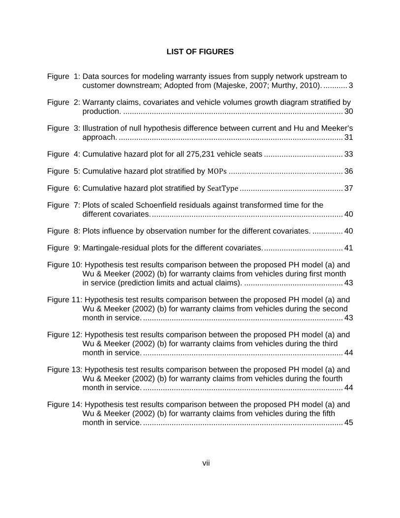
assembled. Figure 1 illustrates some of the major sources of information for developing

early warranty detection models in the automotive industry. This echoes to Murthy’s four

notations of reliability: design, inherent, sale and field reliability (Murthy, 2010). If this

prior upstream information can be utilized in a statistical framework to correlate to

warranty claims, the detection power of an early warranty model might improve. Such

an early warning system can also be used to monitor the effectiveness of corrective

actions. While there is a growing body of literature on warranty modeling and detection,

3

to the best of my knowledge, there is no model in the literature that explicitly links

information from the supplier network to improve early warranty detection.

Figure 1: Data sources for modeling warranty issues from supply network upstream to customer downstream; Adopted from (Majeske, 2007; Murthy, 2010).

My research is motivated by the need for models to explicitly utilize upstream

manufacturing process and quality/testing information from suppliers. With over 10

years of professional experience in the warranty and reliability area with automotive

OEMs and suppliers, I can personally attest to these needs and progressive OEMs are

demanding the same. In the current highly competitive environment, suppliers are being

pushed to improve warranty performance for their responsible subsystems in the

vehicles. When a warranty issue develops in the field, the issue is normally traced from

the top to the bottom of the pyramid structure in Figure 1. In many cases, the

precursors to the issue could be found at suppliers' sites months or even years earlier in

terms of a quality spill, a design error etc. In addition, to address these warranty issues,

suppliers often implement corrective actions without good knowledge for their

Warranty Coverage

Cutoff Date

Vehicle Sold

Vehicle Assembly

Subsystem Assembly

Component Production

Subsystem/Component Pre-production Testing

OEM Production Quality Audit before

Delivery

Suppliers’ Design/Production

Validation Test

Suppliers’ In Plant Repair/Rework

Suppliers End-Of-Line Test

Time(Not to Scale)

Past /Surrogate Programs

Past/Surrogate Program Warranty

Performance

OEM Test Fleet Data

OEM Proving Ground Test

OEM In Plant or Lot Repair

Defects Rejected from OEM

Suppliers’ Design/Process/Material Change

Suppliers’ In Plant Repair/Rework

Suppliers End-Of-Line Test

Defects Rejected from Upper Tier Supplier

Suppliers Design/Process/Material Change

Past/Surrogate Program Quality

History

CustomersOEMs

FieldProductionProductionProductionDevelopment

Transportation

Storage

Usage Intensity

Usage Mode

Operating Environment

Maintenance Actions

Operator’s Reliability

Suppliers

Lower Tiers Upper Tiers

4

effectiveness, leading to instances where the effectiveness is revealed through future

claims to be less than expected. Facing such embarrassing situations, management is

often raising the following sorts of questions:

Can we act on warranty issues more proactively instead of reactively?

Can we estimate our warranty risk early on?

How to verify such a warranty risk quickly?

Once a corrective action is implemented to address a warranty issue, how to

confirm its effectiveness quickly?

In the context of warranty issues, to answer the above sorts of questions, we need to

rethink the pyramid structure of Figure 1 in a different way: improving warranty

performance should start from the bottom of the pyramid to the top whereas

requirements (form, function, and fit) often flow the top to the bottom.

1.2 Research Objectives and Scope

The primary objective of this research is to introduce a statistical modeling

framework that explicitly utilizes upstream supply chain information to: 1) allow early

detection of warranty issues, 2) facilitate early validation of the effectiveness of

corrective actions, and 3) to aid in predicting the warranty claim rates. By utilizing

hazard rate models and further extending it to incorporate Bayesian analysis, upstream

supply chain information is directly linked to expected warranty claims as explanatory

covariates to achieve this goal.

While warranty claims can relate to reliability for the whole product life cycle at

different stages: design reliability due to reliability specification at product development

5

stage, inherent reliability due to assembly errors and component non-conformance, sale

reliability due to damage or deterioration in transportation and storage, and field

reliability due to customer usage mode/intensity and operating environment (Murthy,

2010); warranty claims can also related to human factors such as misuse, neglect, fraud

or lack of training on product operation (Wu, 2011), this research is from a supplier’s

point of view, focuses on linking warranty claim rates to design and inherent reliability,

to which the upstream supply chain information are available and can be extracted and

on which a supplier has a control. However the statistical modeling framework from this

research can easily extended to sale and field reliability by including the available

relevant information as explanatory covariates.

While much of this research focuses on application of the proposed warranty issue

detection models to the automotive industry, the models are also relevant to other

industries that rely on a supply network to build parts of the product.

6

CHAPTER 2 HAZARD RATE MODELS FOR EARLY WARRANTY ISSUE DETECTION USING UPSTREAM SUPPLY CHAIN INFORMATION

2.1 Introduction

This chapter is organized as follows. Section 2.2 reviews relevant literature. Section

2.3 describes the structure of suppliers’ manufacturing and quality/testing data sources

that might be indicative of future warranty claims. Section 2.4 outlines the proposed

methodology of utilizing hazard rate models to correlate upstream data sources to

warranty claims. Section 2.5 develops an enhanced early warranty detection scheme by

incorporating upstream suppliers’ quality/testing data. Section 2.6 reviews the

performance of the proposed method through a case study. Finally, Section 2.7

provides summary remarks and directions for further study.

2.2 Literature Review

Detection of a reliability problem often involves several steps: a) Statistical modeling

of warranty claims so that those factors influencing product reliability can be selected

and the parameters in the model can be estimated; b) Baselines for the parameters are

obtained or predicted from historical warranty claims and/or from subject matter experts

(SMEs) in the absence of any historical information, c) Critical values for the parameters

are set to balance power of detection and false alarm probability, and d) Observed

parameters for the current product model cycle are compared against the critical values

to trigger out-of-control signals.

There is a growing body of literature discussing statistical modeling of warranty

claims. In the automotive industry, as the number of expected warranty claims is often

small under any given failure mode (claim rates are typically measured as claims per

7

thousands of vehicles) compared to the large number of vehicles in field, from a

reliability point of view, such warranty claims are often treated as rare and independent

events, making the Poisson model an appealing statistical model for warranty claims.

Since the seminal paper by (Kalbfleisch et al., 1991) that proposed a Poisson model to

analyze warranty claims, many papers have been authored that focus on predicting

future warranty claims for the remainder of warranty life based on existing/past warranty

claims for the early portion of warranty life. Models have been developed to also deal

with such issues as warranty report delay (Kalbfleisch and Lawless, 1991; Lawless,

1994); (Lawless, 1998), sales delay (Lawless, 1994; Majeske et al., 1997), two

dimensional warranty policy such as 3 years/36,000 miles whichever comes first (Yang

and Zaghati, 2002); (Krivtsov and Frankstein, 2004; Majeske, 2007), treatment of

incomplete data (Hu and Lawless, 1996, 1997; Oh and Bai, 2001; Rai and Singh, 2003,

2004; Mohan et al., 2008), treatment of warranty claims related human factors such as

non-failed but reported (NFBR), failed but not reported (FBNR) and claims from

intermittent failures claims (Wu, 2011). While the vast majority of the literature assumes

that the customer will file at most a single claim for a particular warranty issue/system

and hence the focus on survival analysis methods that experience a single event,

(Lawless, 1995; Lawless and Nadeau, 1995; Fredette and Lawless, 2007) also provided

methods to forecast warranty claims based on a recurring event perspective that allows

the customer to file multiple claims over time for the same system/issue. (Blischke and

Murthy, 1996), and more recently (Karim and Suzuki, 2005; Wu and Akbarov, 2011),

have reviewed the literature on mathematical and statistical techniques for analysis of

8

warranty. The above studies typically serve the purpose of financial planning (warranty

accruals) and taxation.

There is also literature focusing on detecting an emerging quality or reliability

problem by predicting warranty claims for new vehicles (such as vehicles produced in

current production month) based on warranty claims available for older vehicles (such

as vehicles produced in past production months). These early/accurate warranty issue

detection methods can actively reduce warranty cost by facilitating implementation of

corrective actions in time, directly impacting company’s bottom line. In this regard, some

researchers have adopted the Poisson model discussed earlier to model warranty

claims and establish the baseline, then utilizing the conventional statistical process

control techniques to detect emerging quality or reliability problems month by month

either by production or calendar months. (Wu and Meeker, 2002) stratified warranty

claims by vehicle production month and age in terms of months in service (i.e., the

difference between vehicle repair date and vehicle sold date). Assuming that warranty

claims for vehicles from different production months and ages follow independent

Poisson models with different claim rates, they proposed a sequential test procedure for

early warranty detection. Such a scheme generalized the conventional process control

chart by sequentially comparing predefined baseline claim rates from historically stable

production periods to those from current production month for corresponding ages

(available sequentially), so that an emerging quality or reliability problem can be

detected with a predefined Type-1 error (i.e., false alarm error). (Oleinick, 2004)

improved the conventional control chart (u chart) by applying standard reliability growth

9

models to calibrate the variability in the reliability of vehicles among calendar months

not accounted for by conventional reliability bathtub curves.

Another group of researchers adopted computational intelligence techniques such

as artificial neural network methods to model warranty claims. They argue that the

traditional distribution classes may not be flexible enough to capture the failure

distributions observed in actual warranty claims and that qualitative factors are difficult

to incorporate into traditional statistical models, compromising the accuracy required for

early warranty detection. (Lindner and Klose, 1997) and (Lindner and Studer, 1999)

observed that warranty claim rate curves along production months are rather similar for

different ages, but different only in rate level, and they applied machine learning and

neural network models to integrate warranty claim information about the

interdependency between vehicle production month and age, and managed to provide

trend prognoses several months in advance with good accuracy. (Grabert et al., 2004)

estimated warranty claim rates using the multi-layer perceptron model, then, besides

warranty claims, they further include OEM’s quality data such as production audits

before delivery into the analysis to establish the baseline. (Lee et al., 2007) included

qualitative factors such as product type, warranty service area, part significance,

seasons into their study on warning/detection of warranty issues. (Wu and Akbarov,

2011) introduced a weighted support vector regression (SVR) and weighted SVR-based

time series model to forecast warranty claims.

As we look back on the warranty timeline starting from current time (cut-off date) in

Figure 1, a data source pyramid forms along the timeline: towards the top of the

pyramid is the field data from customer (warranty claims) at the vehicle level, available

10

relatively late with scarcity. Towards the bottom of the pyramid is data from suppliers

regarding lower-level components and subsystems, available earliest and abundant. Lot

of this upstream information is available long before a vehicle is built and any warranty

claims are filed. More importantly, since this upstream data is at the level of subsystems

and components, it is more physics and failure mechanism relevant and might help

identify, early on, root-causes of output warranty claims. Vast majority of the extant

warranty detection literature focuses on warranty claims themselves, while few

suggested the utilization of upstream OEM data. For example, (Grabert et al., 2004)

utilize OEM’s plant quality data for warranty detection, with an OEM perspective. To the

best of our knowledge, there is not a single article in the literature that exploits further

upstream data, in particular, the wealth of production quality/testing data from suppliers,

for improved warranty detection. The primary objective of this paper is to address this

short-coming in the literature and propose models that exploit upstream warranty

relevant data sources from suppliers, so that any emerging quality/reliability problem

can be detected earlier with more power.

2.3 Upstream Data Sources for Early Warranty Detection

As OEMs globalize their vehicle production and component sourcing, more and

more suppliers are supplying components/subsystems to multiple OEMs, or to multiple

vehicle platforms within one OEM (platform is a shared set of common

design/engineering efforts and major components over a number of outwardly distinct

models). Therefore, warranty detection has become more complex requiring increased

active involvement from suppliers. To meet these requirements, OEMs cascade vehicle

11

level warranty down to subsystem/component levels, which is often the responsibility of

suppliers. These joint responsibilities and objectives are defined by warranty

agreements and warranty sharing programs. To support this process, the Original

Equipment Suppliers Association (OESA) drafted “Suppliers Practical Guide to

Warranty Reduction” in 2005 (OESA, 2005) and later published in 2008 through the

Automotive Industry Action Group (AIAG) as (AIAG, 2008). In recent years, the warranty

reduction focus has shifted from warranty cost settlement or transfer to preventing or

quickly and effectively eliminating reliability problems, which has greatest impact on

warranty cost reduction in the long-term. To assist suppliers in meeting the warranty

objective, OEMs typically allow suppliers to access their warranty claims database,

warranty returned parts from end customer, test data from proving ground or test fleet

vehicles, and plant audit and quality data. Some OEMs even allow suppliers to call

dealer technicians within days of a claim to better link failure-modes to warranty claim

data. All these initiatives provide suppliers with a great opportunity to correlate and

exploit their internal quality/testing data (“Suppliers” in Figure 1), to OEM data (“OEMs”

in Figure 1) to warranty claims (“Customer” in Figure 1).

2.3.1 OEM Warranty Data Sources/Structure

The structure of OEM warranty data has been explained in detail by (Wu and

Meeker, 2002). It is worth noting that the key for this data structure is the vehicle

identification number (VIN). From VIN, we can trace the vehicle built date, repair date,

and all other vehicle production and warranty repair related information. More

importantly, as will be explained later, using VIN, we can also trace back to production

related information from suppliers responsible for components/subsystems. While the

12

literature discusses warranty data complications associated with claims reporting delays,

including (Wu and Meeker, 2002), fortunately, this is no longer an issue because of

effective and near real-time IT integration of dealer network and repair shops to OEM

warranty database systems. Given that suppliers have direct electronic access to this

database, they can also obtain warranty claims related to their responsible

subsystems/components without delay.

2.3.2 Supplier Network Warranty Data Sources/Structure

Modern production information technology and extended Enterprise Resource

Planning (ERP) software is equipping OEMs and suppliers with enhanced warranty

traceability, i.e., the ability to link upstream production quality/testing data to the

warranty process timeline in Figure 1. We illustrate this using a typical Tier-1 supplier’s

production example. A typical Tier-1 supplier’s production process starts first from

receiving a VIN specific bill-of-material (BOM) from the OEM vehicle assembly plant.

These BOMs are sent from OEM’s production system to suppliers’ production system

electronically (typically, using some form of an electronic data interchange (EDI)

system). The BOM defines the configuration/options for the supplier’s subsystem for

each VIN. For example, in the case of a seating supplier, the BOM will identify seat

model type, material (leather/fabric), and optional content (e.g., active head-restraints,

heated seats). Upon receiving the BOM, the supplier’s production system typically

generates a unique sequence number for the subsystem corresponding to each VIN.

These sequence numbers are then sent to the first station of the supplier’s assembly

line for building the desired subsystem. At each station of the assembly line, certain

components are added and then tested against production specifications by measuring

13

functional parameters such as noise, current, voltage, resistance, speed, count etc. For

key components, their unique identification numbers, typically part of bar codes, are

also scanned into the production system before test; this provides the traceability from

Tier-1’s sub-system to lower tiers’ components. If any measurement is out of

specification, the in-process subsystem is rejected and the assembly line is stopped

until the problem is fixed. This process will repeat for each station until the subsystem

corresponding to the sequence number is completely built and passes all the function

tests for all stations. Finally, the subsystem is put on a shipping rack ready for shipment

to OEMs’ vehicle assembly plant. As each sub-system is built, all its function test results

and component scan results are stored in the production database, tied to sub-system

sequence number and VIN, and are available for access. As each sub-system may

consist of many components, an assembly line may consist of many stations and each

station may conduct many test and scan activities, the amount of data stored is huge

but rich: for annual production of 200K vehicles, a typical Tier-1 supplier’s production

database stores millions of records for its responsible subsystems. Likewise, the

production data collection process can be cascaded down to lower tier suppliers.

Therefore, suppliers’ production database has a wealth of information that can support

early warranty detection:

1. The core element of the production database is strong traceability. It uniquely

maps each vehicle unit (VIN) to its corresponding subsystem (sequence number),

then from the sequence number, it uniquely maps the subsystem to its

components (through bar codes). From VIN, sequence number and bar code,

14

quality data from suppliers’ production such as production date, function test

results can be directly linked to vehicle warranty claims.

2. Since warranty detection methods can benefit from specific information regarding

the failure mechanisms, including manufacturing, production/quality data from

suppliers’ production database can aid these detection methods.

3. Unlike OEMs’ production quality audit, which typically samples 1% of the sub-

systems that enter vehicle production (Grabert et al., 2004), suppliers’ production

databases often provide a complete history on 100% of the sub-systems (for all

vehicles with and without warranty claims).

4. Despite its huge amount of information, it is well organized and structured,

allowing us ready access to information critical for warranty detection.

Besides function test data, a typical Tier-1 supplier also stores information regarding

units rejected by the OEM to its production database. After the subsystems are shipped

to OEMs’ vehicle assembly plant, some of them may be rejected by OEMs due to

defects and shipped back to suppliers. Suppliers may repair them by rework or replace

them. The sequence numbers and related events are then recorded in the production

database.

In addition to function test data and customer quality audit/reject data, suppliers also

have other quality/testing data that may be linked to warranty claims. Examples of such

information include:

Number of quality alerts generated each month due to defects found in OEM’s

plant

Process capability information (e.g., ) from all stations (by week/month)

15

Internal scrap/rework rates (by date/batch)

Component reject rates (by date/batch)

Process and design change history (during production phase)

Design and production validation test history (during development phase)

Historical warranty claims and quality/testing data from similar subsystems on

different vehicle lines or different OEMs

The extant literature is quite lacking in offering early warranty detection methods that

can exploit the wealth of such upstream production quality/testing information. The

primary objective of this manuscript is to propose methods that can begin to address

this gap.

2.4 Correlating Upstream Quality/Testing Data to Warranty Claims

In the recent literature, a popular approach to modeling warranty claims is a

nonparametric approach based on warranty claim counts modeled with a Poisson

distribution with claim intensities that depend on production period and number of

periods in service. The other standard assumption following the statistical model used

by (Kalbfleisch and Lawless, 1991) is that the claims for vehicles from production period

and periods in service (for the particular subsystem or labor code under

consideration) can be described as independently distributed Poisson random variables.

(Wu and Meeker, 2002) argue that this probability model is strongly supported by most

warranty applications where there is a large number of units in the field, but the

occurrence of any given failure mode, when reliability is as expected, should be rare

and statistically independent from unit to unit. However, to reduce the need for

16

estimation of a (potentially) large number of report intensity parameters for each

production period and number of periods in service for each sub-system or labor code

(which can run into thousands), we directly model the claim rate as a hazard function

over service age (herein simply referred to as age) for each production period .

This not only reduces the need for independent estimation of a large number of report

intensity parameters for each period in service but also allows us to avoid the need for

the assumption of independently distributed Poisson random variables. Instead, we

propose the more exact Binomial distribution to model warranty claims for each sub-

system or labor code. In addition, while (Wu and Meeker, 2002) employ a

nonparametric approach for modeling warranty claims over fitting a standard parametric

distribution such as a Weibull or a lognormal distribution for each subsystem or labor

code, given the challenges associated with identifying the right model for each of the

hundreds to thousands of subsystems and labor codes of interest, our proposed method

fully supports both a nonparametric as well as a parametric treatment of the hazard rate

function.

We use the claim rate function to estimate the probability that any

individual vehicle unit from production period will generate a claim (for the particular

labor code or sub-system) by age :

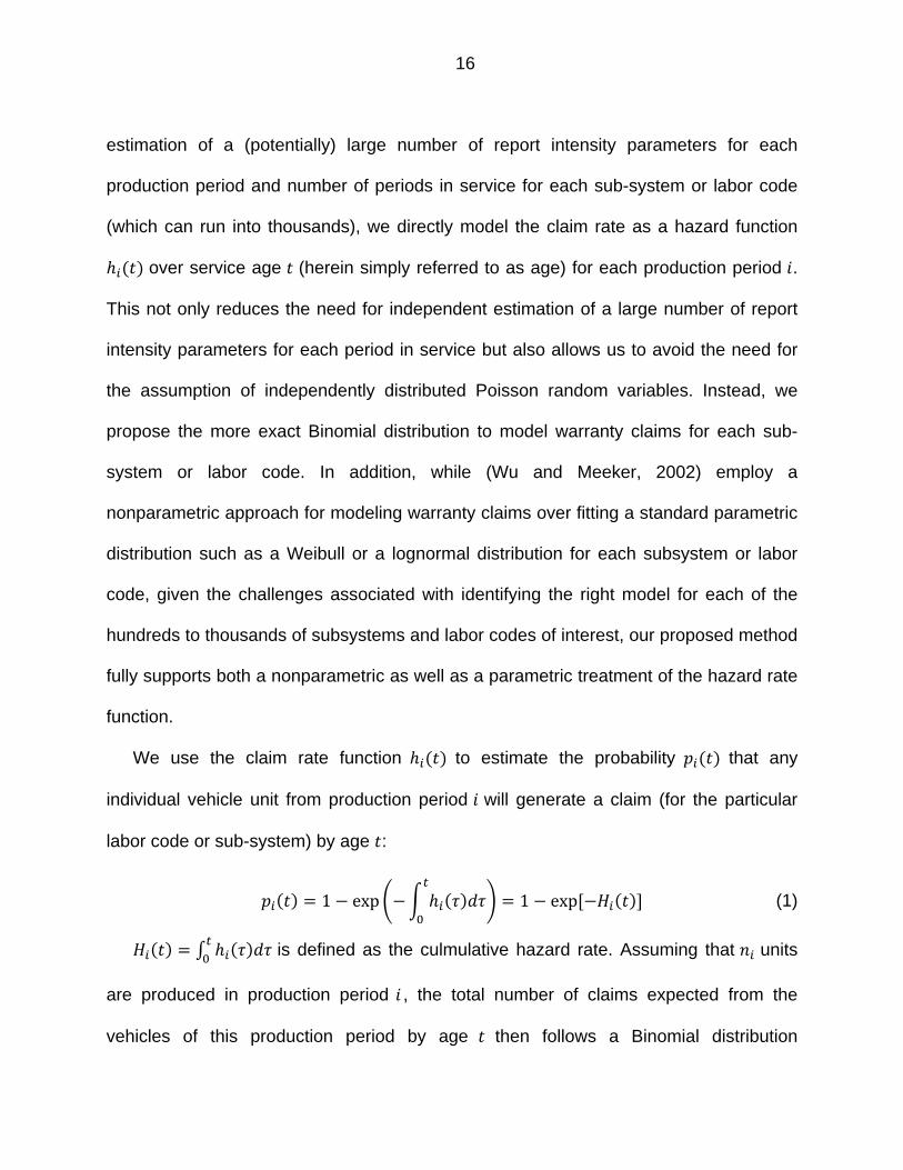
1 exp 1 exp (1)

is defined as the culmulative hazard rate. Assuming that units

are produced in production period , the total number of claims expected from the

vehicles of this production period by age then follows a Binomial distribution

17

, . In the sections that follow, we also outline a method that eliminates the

need for separately estimating the hazard rate function for each production period

through the use of production month covariates based on upstream supply chain

information.

In order to correlate upstream supply chain quality/testing information with warranty

claim rate, we propose the use of hazard rate models. By treating upstream supply

chain quality/testing information as explanatory covariates of warranty claim rate, we

directly link warranty claims with them. Even though one can use conventional models

such as linear regression, log-linear regression, logit, probit and inverse polynomials

analysis, the special properties of warranty claims make these models inappropriate

due to their inefficiency, bias, inconsistency and insufficiency. Warranty claim data are

heavily right censored (>90%); the conventional models can lead to biased estimates of

the covariate effects by not incorporating this available censoring information (Hardin

and Hilbe, 2007). In addition, if the explanatory covariates associated with warranty

claims are time dependent (such as product usage rates/patterns), the conventional

models have difficulty handling these situations. Note however that time dependent

covariates are not considered in this manuscript and will be the focus of future work.

Literature from other research areas such as marketing and political science (King,

1988; Helsen and Schmittlein, 1993; Soyer and Tarimcilar, 2008) confirm the above

limitations of conventional models on certain datasets which share a lot of the same

properties as warranty claims, and demonstrate that hazard rate models are able to

overcome these limitations and outperform conventional models in terms of estimate

stability and predictive accuracy.

18

2.4.1 Hazard Rate Models

Hazard rate models can be approached a number of ways. Since the seminal work

by Cox on the so called proportional hazard (PH) models (Cox, 1972; Cox, 1975), they

have been extensively used in survival analysis to provide a statistically rigorous

estimation and prediction of survival rates based on explanatory covariates (Klein and

Moeschberger, 2003; Lawless, 2003; Li et al., 2007). There are also a number of non-

proportional hazard rate models, with a popular option in survival analysis being the

accelerated failure time (AFT) model. Whereas a PH model assumes that the effect of a

covariate is to multiply the hazard by some constant, AFT model assumes that the

effect of a covariate is to multiply the predicted event time by some constant. For a

detailed discussion on the choices and tradeoffs for hazard models and their parameter

estimation processes, see (Lawless, 2003; Hosmer et al., 2008). In what follows, we

employ the PH model for linking warranty claim rates to upstream supply chain

quality/testing information. However, the methodology is equally relevant if an alternate

hazard rate model is employed.

2.4.2 Proportional Hazard (PH) Model

Let denote the hazard rate extracted from warranty claims corresponding to a

subsystem or labor code for which a supplier is responsible. The subsystem’s can

be calculated from OEM’s warranty database by selecting the first claim for each VIN

under a chosen set of labor codes or defect codes defined by OEM’s warranty database

(given our interest here in early warranty detection, the focus here is on the first claim

and not repeat claims). Let | denote the hazard rate for the subsystem of interest

19

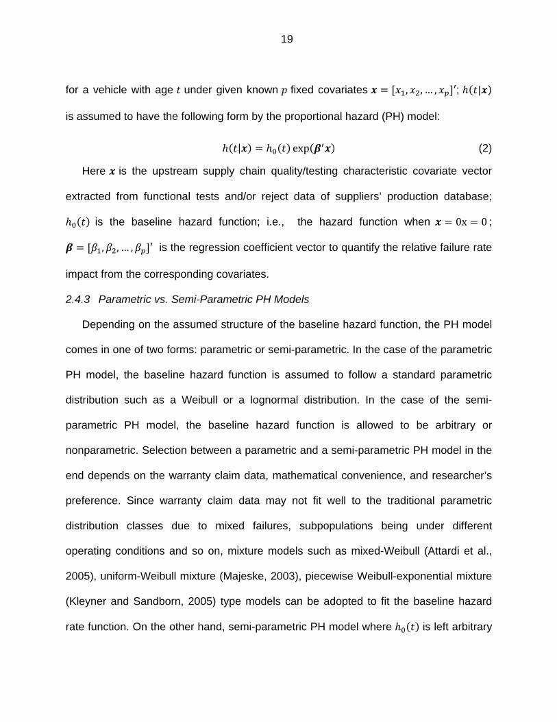
for a vehicle with age under given known fixed covariates , , … , ′; |

is assumed to have the following form by the proportional hazard (PH) model:

| exp (2)

Here is the upstream supply chain quality/testing characteristic covariate vector

extracted from functional tests and/or reject data of suppliers’ production database;

is the baseline hazard function; i.e., the hazard function when 0x 0 ;

, , … , ′ is the regression coefficient vector to quantify the relative failure rate

impact from the corresponding covariates.

2.4.3 Parametric vs. Semi-Parametric PH Models

Depending on the assumed structure of the baseline hazard function, the PH model

comes in one of two forms: parametric or semi-parametric. In the case of the parametric

PH model, the baseline hazard function is assumed to follow a standard parametric

distribution such as a Weibull or a lognormal distribution. In the case of the semi-

parametric PH model, the baseline hazard function is allowed to be arbitrary or

nonparametric. Selection between a parametric and a semi-parametric PH model in the

end depends on the warranty claim data, mathematical convenience, and researcher’s

preference. Since warranty claim data may not fit well to the traditional parametric

distribution classes due to mixed failures, subpopulations being under different

operating conditions and so on, mixture models such as mixed-Weibull (Attardi et al.,

2005), uniform-Weibull mixture (Majeske, 2003), piecewise Weibull-exponential mixture

(Kleyner and Sandborn, 2005) type models can be adopted to fit the baseline hazard

rate function. On the other hand, semi-parametric PH model where is left arbitrary

20

(non-parametric) offers considerable flexibility to support arbitrary failure

modes/mechanisms and freedom from any shape/scale constraints (Helsen and

Schmittlein, 1993). We do note that this added flexibility comes with some risk in that

the hazard rate estimation is relatively more vulnerable to noise in the data (which might

lead to ‘artificial’ fluctuations in hazard rate). However, given that warranty monitoring

often involves very large datasets, this risk is bounded. The major assumption for all PH

models is that the multiplicative or log-additive hazard structure from Eq.(2) is correct.

Such an assumption needs to be validated formally and is discussed in later sections.

2.4.4 Estimating PH Model Parameters from Past/Current Warranty Datasets

Let be the number of vehicles for which there exists a partial or full warranty claim

history. The censored service age life times , , 1, … , , and corresponding

covariate vectors are assumed to be known for each vehicle . The indicator variable

1 if the th vehicle experienced a warranty claim for the subsystem or labor code of

interest at service age , 0, if the th vehicle has not produced any warranty claim

until age . Using the warranty dataset, one could estimate the baseline hazard function

and covariate effects through maximum likelihood estimation (MLE) procedures.

Depending on whether we employ a fully parametric or semi-parametric PH model, here

is the process:

1. If the baseline hazard function can be represented by one from some family

of parametric models with parameter vector with form ; , then the full log-

likelihood function will apply (Lawless, 2003):

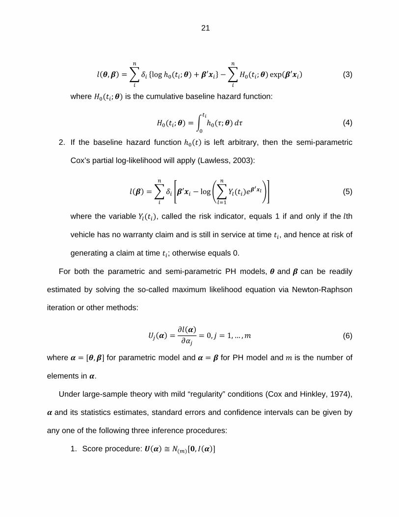
21

, log ; ′ ; exp ′ (3)

where ; is the cumulative baseline hazard function:

; ; (4)

2. If the baseline hazard function is left arbitrary, then the semi-parametric

Cox’s partial log-likelihood will apply (Lawless, 2003):

′ log (5)

where the variable , called the risk indicator, equals 1 if and only if the th

vehicle has no warranty claim and is still in service at time , and hence at risk of

generating a claim at time ; otherwise equals 0.

For both the parametric and semi-parametric PH models, and can be readily

estimated by solving the so-called maximum likelihood equation via Newton-Raphson

iteration or other methods:

0, 1, … , (6)

where , for parametric model and for PH model and is the number of

elements in .

Under large-sample theory with mild “regularity” conditions (Cox and Hinkley, 1974),

and its statistics estimates, standard errors and confidence intervals can be given by

any one of the following three inference procedures:

1. Score procedure: ≅ ,

22

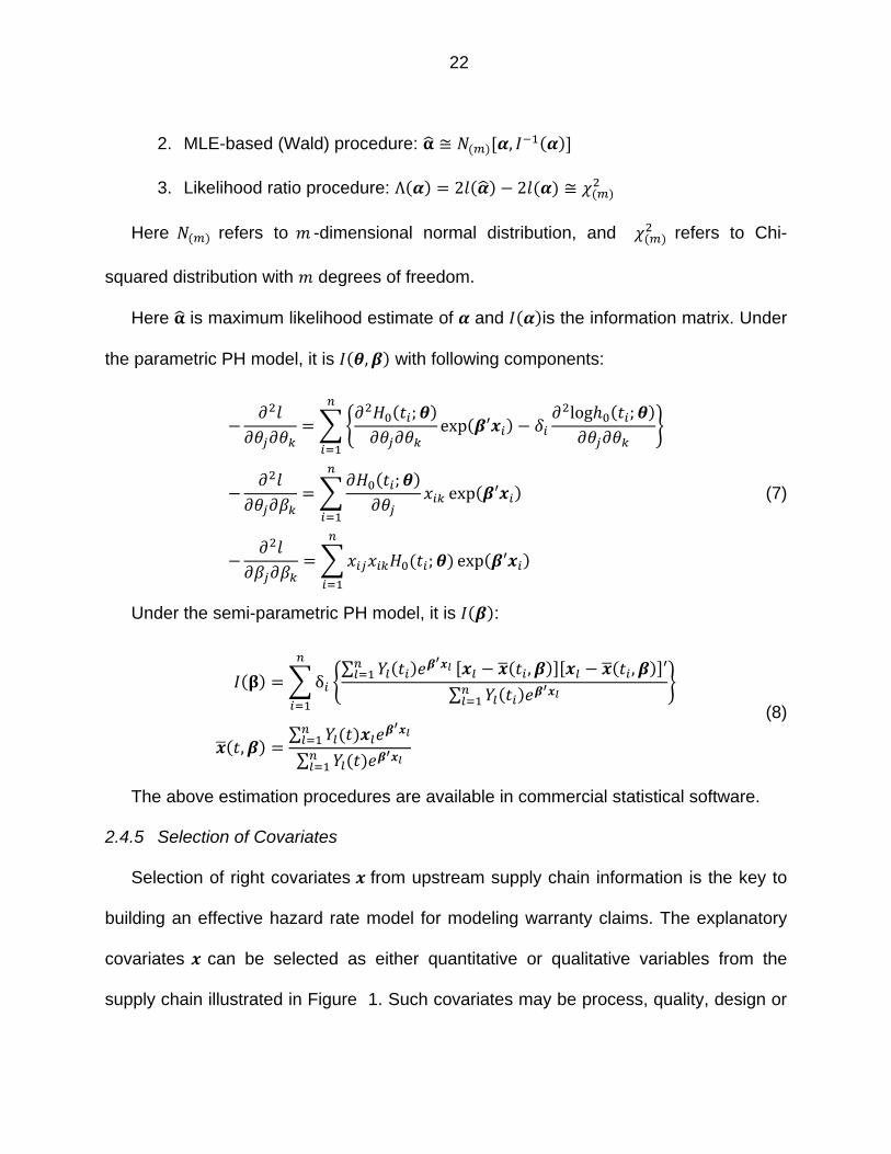
2. MLE-based (Wald) procedure: ≅ ,

3. Likelihood ratio procedure: Λ 2 2 ≅

Here refers to -dimensional normal distribution, and refers to Chi-

squared distribution with degrees of freedom.

Here is maximum likelihood estimate of and is the information matrix. Under

the parametric PH model, it is , with following components:

;exp ′

log ;

;exp ′

; exp ′

(7)

Under the semi-parametric PH model, it is :

δ∑ , , ′

∑

,∑

∑

(8)

The above estimation procedures are available in commercial statistical software.

2.4.5 Selection of Covariates

Selection of right covariates from upstream supply chain information is the key to

building an effective hazard rate model for modeling warranty claims. The explanatory

covariates can be selected as either quantitative or qualitative variables from the

supply chain illustrated in Figure 1. Such covariates may be process, quality, design or

23

product related. They may be from the production database that ties to VIN or from

other heterogeneous sources that may only be available in aggregate form. The

selection depends on the application and the kind of warranty issues that need to be

detected:

If a significant “process deterioration or improvement” is sensed, and its impact

on warranty performance is desired to be detected, process related covariates

such as quantitative variables noise (dB), current, voltage, resistance, speed,

count etc. or qualitative variables such as pass/fail could be selected from

functional test results extracted from a supplier’s production database.

If a significant “quality deterioration or improvement” is sensed, and its impact on

warranty performance is desired to be detected, quality related covariates such

as customer reject data in terms of reject rate or defective parts per million (PPM)

could be selected from functional test results extracted from a supplier’s

production database.

If there is a design or material change being implemented to address a previous

reliability problem or reduce cost, and if we hope to evaluate the effectiveness of

such a corrective action, we may apply qualitative coded covariate 0 1

x 0 x 1 to VINs before and after the corrective actions correspondingly. If we

have validation test results such as a life-testing Weibull plot to demonstrate the

reliability improvement, we may apply a quantitative covariate such as the

Weibull location parameter α α α α to VINs before and

after the corrective actions correspondingly.

24

If we want to monitor the overall warranty performance for the subsystem a

supplier is responsible under known current process, quality and design

conditions, we may include all of the above possible covariates.

2.4.6 PH Model Development

Evaluation of the regression coefficients of the covariates (i.e., ) in Eq.(2) requires

a reasonably large training dataset to achieve considerable accuracy due to large-

sample theory (Cox and Hinkley, 1974). If current production vehicle model has

significant history or is a carryover model from prior years, normally abundant historical

warranty claims exist to form the PH model training dataset. If current production vehicle

model is a newly launched vehicle model, the historical warranty claims from

surrogate/similar vehicle models may be used to form the training dataset. If historically

a supplier supplied similar subsystems for different vehicle models to either the same

OEM or different OEMs, such historical warranty claims can be tailored or calibrated to

form a surrogate training dataset by considering different applications, customer usage

and operating conditions on the newly launched vehicle model.

Initially, we may include all covariates believed to impact , based on engineering

experience and judgment, in developing the PH model. In reality, not all of the

covariates might prove to be statistically significant in impacting due to

heterogeneity in customer usage and/or operating conditions. For example, certain

features of the subsystem are seldom used by customers or the subsystem is seldom

operated under certain conditions. Under such situations, it may take a long time for

certain covariates to demonstrate their impact on . Also, not all candidate covariates

are independent explanatory variables to . Forward and backward stepwise

25

selection procedure (Klein and Moeschberger, 2003) can be applied to sequentially

remove confounding and statistically insignificant covariates to arrive at a final

candidate multivariate PH model. Such covariate screening process may take several

iterations in association with good engineering experience and judgment.

For covariates without any history, such as a major design/process change to

address a previous reliability problem, the corresponding model coefficient cannot be

evaluated due to the lack of a training dataset representative of vehicles that

incorporate the design change. In such cases, PH model has to be extended to

incorporate Bayesian analysis which will be discussed in Chapter 3.

2.5 Early Warranty Detection Scheme

Once the PH model is established and validated, we are ready to set up the

warranty issue detection rule and conduct formal hypothesis tests. Early warranty

detection scheme monitors warranty claims, vehicle service age, and supply chain

quality/testing covariates over the vehicle production life cycle. The vehicle production

period is often stratified by date, week or month depending on the monitoring frequency,

and so are the warranty claims, vehicle service ages, and covariates.

2.5.1 Notation and Assumptions

In our study, we define the beginning of life of the subsystem to be the time when its

vehicle was produced (if appropriate, one can also use the time of production of the

subsystem to be the starting point). Hence, for vehicles that produced a warranty claim

on the subsystem or labor code of interest, the non-censored life of the subsystem ( in

Eq.(2)) is the difference between the date of repair/diagnosis and the vehicle production

26

date; for vehicles without a warranty claim it is the difference between the most current

monitoring date and the vehicle production date. Although other definitions could be

employed (e.g. vehicle sold date which coincides with the beginning of the warranty

period), this definition provides convenience for suppliers: sales information (which

provides vehicle sold dates) is only available to suppliers on vehicles with warranty

claims from the OEM warranty claims database (this information is generally not

available for vehicles without warranty claims). Also, the defined starting time can

coincide with suppliers’ subsystem production date, especially for Tier-1 suppliers that

build their respective subsystems in “Just-In-Time” (JIT) plants nearby OEMs’ vehicle

assembly plant; individual vehicle units might be built within a day or two of when its

subsystems are built. Moreover, before a vehicle is sold, dealers conduct routine pre-

delivery inspections and any defect or failure noticed will be reported as a warranty

claim to OEMs’ warranty claims database, so that the warranty claims include sale

reliability due to possible transportation damage or deterioration. For our study, since

this definition assumes that vehicles are produced and enter service on the same date,

it avoids the complications of sales delay analysis (which might be necessary in some

cases).

Following the notation from (Wu and Meeker, 2002), let denote the number of

vehicles produced in period and denote the number of first warranty claims during

th period in service for units that are manufactured in period . Since there is no

warranty claim report delay these days in OEM warranty databases (due to direct

computer entry through OEM’s dealer network), first becomes available in period

.

27

2.5.2 Binomial Distribution Model for Monitoring Warranty Claims

As stated in 2.4, we propose the Binomial distribution model to model warranty

claims. We treat as an independently distributed Binomial , random variable,

where represents the probability that the subsystem of interest manufactured in

period will produce the first warranty claim during the th period in service. The

reference value for , denoted by , can be obtained from (1) as:

exp 1| exp | (9)

where is the fixed covariate vector for production period and | is the

cumulative hazard rate until the th period in service. Once is known, the upper and

lower confidence limits of , and , respectively, can be easily calculated from the

Binomial distribution.

To evaluate | for a supplier’s subsystem, warranty claims for a chosen (set) of

categorization codes are extracted from OEMs’ warranty database. Each code

represents causal component of a vehicle and the kind of repair taken, and all codes

are structured in function groups. To have better statistical reliance and reduce the

probability of the code being wrongly binned by dealers, we cluster a group of codes to

represent a supplier’s subsystem so that even if a component repaired is binned to a

wrong code, the wrong code still falls in the chosen group of codes with high possibility

due to its local or functional relation to the causal component.

Our study focuses on early detection of a warranty issue, normally within 12 months

after a vehicle is produced. Hence, the issue of warranty “drop-out” due to two-

dimensional warranty policy is not a problem here when compared to OEMs’ 36

28

months/36,000 miles or even 60 months/60,000 miles warranty policies typical in North

America. Moreover, as (Wu and Meeker, 2002) pointed out, the warranty “drop-out” due

to accumulated mileage will be reflected in the PH model through the historical training

dataset.

The vehicles in the field may be subject to heterogeneous environment/usage and

our model captures the variability through the model training dataset. By assuming that

the variability is stable over each production period, our PH model can focus on

variability in the reliability of the manufactured subsystem from the upstream supplier

chain over production periods.

2.5.3 Hypothesis Test

Along the lines of (Wu and Meeker, 2002), the formal problem of detection can be

formulated as a test of the multiple-parameter hypothesis:

: , , … , , … ,

: … ,

(10)

where is the pre-specified number of future periods for which the Binomial distribution

probabilities will be monitored for units manufactured in any given period. For a given

overall false alarm rate, increasing will require a reduction in power to spread

protection over a larger number of monitoring periods.

Consider production period . In this period, units were manufactured and sold. At

the end of production period since all covariates associated with production period i

are available, the claim probabilities , , … , can be predicted from Eq.(9) for all

periods in service. Among these, there were warranty reports during their first

29

period of service, and these reports first became available in period 1. Note that

~ , , and in period 1 , we can test only versus ; no

information is available on , … , . In general, in period , periods after the units

in the th production period were produced, we can test the joint hypothesis of whether:

… , ,

, , , , … , ,

… … … …, ,

For testing , only the , 1,2, … are relevant; the other contains no

information about . Formally, the binomial variables and are not

independent, but through the standard "Poissonization" in large samples, they are

almost independent for any practical purpose. Therefore testing : ,

, … , , … , versus : for some 1,2, … , can be done by

testing, individually, : versus : for 1,2, … , .

Consider first testing : versus : , the warranty claim probability

for a vehicle produced in period for the first period in service. In period 1, we

conclude that if or for some critical values and (to be

determined). Similarly, for testing : versus : (the warranty claim

probability for a vehicle produced in period for the th period in service), in period ,

we conclude that if or for some critical values and (to

be determined).

The primary difference between our hypothesis tests and those from (Wu and

Meeker, 2002) is that their null hypothesis is “static” and is generally expected to be

30

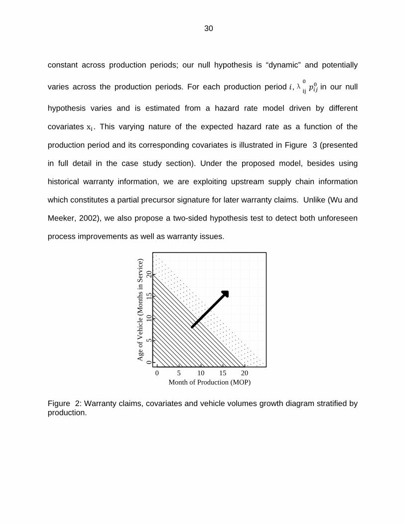
constant across production periods; our null hypothesis is “dynamic” and potentially

varies across the production periods. For each production period ,λ in our null

hypothesis varies and is estimated from a hazard rate model driven by different

covariates x . This varying nature of the expected hazard rate as a function of the

production period and its corresponding covariates is illustrated in Figure 3 (presented

in full detail in the case study section). Under the proposed model, besides using

historical warranty information, we are exploiting upstream supply chain information

which constitutes a partial precursor signature for later warranty claims. Unlike (Wu and

Meeker, 2002), we also propose a two-sided hypothesis test to detect both unforeseen

process improvements as well as warranty issues.

Figure 2: Warranty claims, covariates and vehicle volumes growth diagram stratified by production.

Month of Production (MOP)

Age

of

Veh

icle

(M

onth

s in

Ser

vice

)

0 5 10 15 20

05

1015

20

31

Figure 3: Illustration of null hypothesis difference between current and Hu and Meeker’s approach.

2.5.4 Allocation of False Alarm Probability and Power for Detection

Let be the nominal false alarm probability for testing the sub hypothesis

versus about , corresponding to the th period in service for units from production

period . If we set the overall false alarm probability as , from Boole’s inequality,

∑ , taking the conservative case, we have:

(11)

To balance between quick detection and the overall probability of detection (power)

over potential reliability problems over the first periods of a unit’s life, we follow (Wu

and Meeker, 2002) and choose to be proportional to the information available for

testing versus (this information is proportional to the expected number of reports

during the th period in service). Since age is here defined as the difference between

MOP

Haz

ard

Rat

e at

6 M

onth

s in

Ser

vice

5 10 15 20 25

Current ApproachWu and Meeker's Approach

32

warranty repair date and vehicle production date and instead of the difference between

warranty repair date and vehicle sold date, and we don’t have the implication of sales

delay problem:

(12)

From Eqs.(11) and (12), can be approximated by:

…, 1,2, … , , (13)

Note that unlike (Wu and Meeker, 2002), the nominal false alarm probability for

testing is different here in ages but same for each ; sinceλ is different for

each production period , is different for both production period and

age . This is due to the “dynamic” nature of our null hypothesis H H . Once is

determined, the critical values for carrying out the hypothesis tests, C and , can

be easily calculated from the Binomial distribution.

2.6 Case Study

In order to illustrate and test our statistical framework for early warranty issue

detection, we used a Tier-1 automotive seating supplier as an example. To illustrate the

monitoring scheme from section 2.5, we follow the OEMs’ typical practice of monthly

monitoring frequency and define production period as a production month .

Accordingly, vehicle ages, warranty claims and covariates are also stratified by month.

2.6.1 Data

Two datasets are collected retrospectively:

33

1. Warranty claims dataset is collected from the supplier’s OEM customer warranty

database for supplier’s seat related warranty claims

2. Production dataset is collected from the seat supplier’s plant production database

from which covariates can be extracted.

The two datasets are linked through VIN and can be used to estimate | . In our

case, they cover 275,231 vehicles and 550,462 seats (one driver and one passenger

seat for each vehicle) spanning over 25 production months, 3 model years with each

vehicle having at least 9 months of age. The warranty claim dataset contains 11,915

(4.3%) non-censored data (warranty claims) and 263,316 (95.7%) censored data

(vehicles that did not experience any seat related warranty claim). The large sample

size facilitates us to effectively estimate the PH model. The non-parametric Fleming-

Harrington (FH) estimation of the cumulative hazard plot (Figure 4) for all 275,231

vehicles shows a very smooth line with narrow 95% confidence bands. For confidential

reason, the actual cumulative hazard rate is masked to protect proprietary information

but kept as the same scale as Figure 5 and Figure 6 for relative comparison.

Figure 4: Cumulative hazard plot for all 275,231 vehicle seats

Life(Days)

Cum

ulat

ive

Haz

ard

100 200 300 400 500 600

34

Since this vehicle model has 60 months/60,000 miles warranty policy, the maximum

time in service for this dataset is 1,033 days, so the early warranty claim dataset will not

be affected by warranty drop out due to accumulated mileage. Since the warranty claim

dates are recorded by day, even though the monitoring frequency is defined as monthly,

to maintain the claim date resolution, estimations are based on the actual claim

dates and not by monthly groupings.

2.6.2 Covariates

The production dataset contains in total 27 million function test results for the

550,462 seats. For each seat, there are about 60 function tests depending on the seat

type. The 63 covariates are stratified by production month and extracted from

supplier’s production database:

Monthly process capability indices ( ) for function tests - quantitative

covariates: These are process state indicators for each of the 60 function tests.

1, 2, 3and4 - qualitative covariate: Is an indicator variable that

identifies the type of seat going into the vehicle. The supplier’s plant produced

four different seat types from low end (#1) with fewer features and base material

to high end (#4) with more features and premium material. Higher end seats with

more features/content are expected to have a higher warranty claim rate.

NOKFstN - quantitative covariate: Denotes the fraction of seats, by

month, that did not pass at least one of the function tests in the first pass. This is

the aggregate indicator for overall process state. Before each seat is shipped out

from the supplier’s plant, it has to pass all the 60 function tests either by repair or

replacement. Even though function tests can catch all of the defects exhibited

35

during function testing, they may not catch certain defects such as intermittent

defects which may not show up during functional testing but show up later in the

field. Higher levels of indicate higher risk of warranty claims.

- quantitative covariate: Denotes the fraction of seats rejected by the

OEM vehicle assembly plant, by month, due to various seat defects. This is again

an aggregate indicator for various seat defects either not covered by function

tests or not caught by function tests. Higher levels of indicate higher risk

of warranty claims.

2.6.3 Model Estimation

The initial candidate covariates are , , ,

1, 2, … , 60 . x SeatType, RejectN, NOKFstN, Cpk1, Cpk2,… , Cpk60 These

covariates are chosen due to their direct traceability from supplier system to end

product (seats to vehicles). The particular seat system under consideration is a

“carryover” design from a previous model year without any major design change. Hence,

the covariates reflect well the impact of the manufacturing process on warranty

performance for this supplier’s plant.

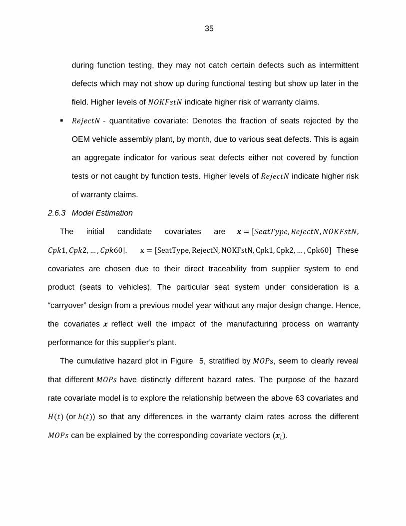
The cumulative hazard plot in Figure 5, stratified by s, seem to clearly reveal

that different have distinctly different hazard rates. The purpose of the hazard

rate covariate model is to explore the relationship between the above 63 covariates and

(or ) so that any differences in the warranty claim rates across the different

can be explained by the corresponding covariate vectors ( .

36

Figure 5: Cumulative hazard plot stratified by MOPs

We use warranty claim and production datasets from 1 MOP 1 to 20 as

training dataset to construct the PH model and estimate regression coefficients of

covariates . This training dataset is represented by solid lines in Figure 2. The training

set has a total of 206,412 vehicles with 4,093 non-censored data (warranty claims) and

202,319 censored data (vehicles never experience any seat related claims). The data

from the remaining five production months, 21 to 25 , are used to form the

detection dataset to conduct sequential hypothesis tests. The detection dataset is

represented by dotted lines in Figure 2.

To construct PH model for this case study, the baseline hazard function h t is

left arbitrary, and we employed Cox’s partial log-likelihood procedure for estimating the

same (available from most statistical software).

It is possible that not all of the 63

covariates , , , 1, 2, … , 60 are statistically

significant in impacting the claim rate . The screening process is to find the

significant covariates. Past experience from the plant tells us that and

Life(Days)

Cum

ulat

ive

Haz

ard

100 200 300 400 500 600

37

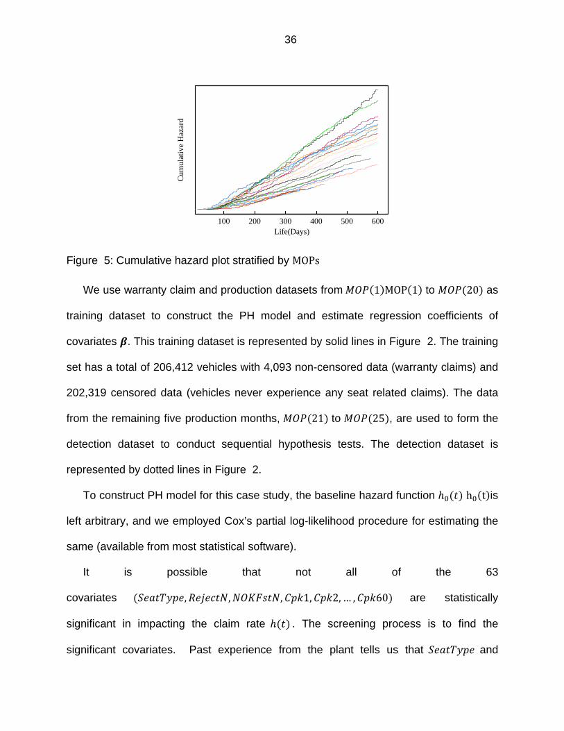
are important covariates: normally when plant produced higher percentage of

high end seats, the warranty claim rate was higher due to reasons explained above.

The non-parametric FH estimation of cumulative hazard plot with 95% confidence band

(Figure 6) stratified by clearly shows the significantly different hazard

functions for the four seat types. Also, whenever the plant received higher customer

rejects , later such defects showed up in warranty. The Wald test on the

single covariate and confirms its significance with 1.4 10

p 1.4 10‐ p 1.4 10‐ and 0 correspondingly.

Figure 6: Cumulative hazard plot stratified by SeatType

We use and as the primary covariates. As for the remaining

covariates, we only retained and the 40 process capability covariates ( )

that exhibited a value of less than or equal to 2.0 in any month of the training dataset

(by definition of process capability, the higher the , the lower the risk of a defect).

These 41 covariates are candidates for the standard forward model construction

procedure under the Akaike information criterion (AIC)(Akaike, 1974):

Life(Days)

Cum

ulat

ive

Haz

ard

100 200 300 400 500 600

SeatType1SeatType2SeatType3SeatType4

38

2log 2 (14)

where is the number of covariates in the PH model and is the likelihood of the model.

The forward procedure is conducted as follows:

1. Include only primary covariates , to fit the PH model, compute

its AIC and set it as the original model.

2. Add an additional covariate one by one from the 41 covariates to the original

model to construct 41 1st iteration models and compute AICs. Compare the

smallest AIC among them with the original model’s, if this AIC is smaller than the

original model’s, update this model as the original model.

3. Repeat step 2 until no more covariates can be added.

After creating a multivariate PH model by the above procedure, a backward

procedure is applied to remove any covariate with 0.05 and keep covariates with

sound physical effect on the PH model. did not prove to be a significant

covariate due to its strong correlation with some of the 60 s. Since is an

aggregate indicator for the 60 s, it becomes redundant.

The model diagnosis revealed that there is a strong interaction between covariate

and time/age, which invalidates the PH model assumption. In order to

account for this interaction in the PH model, we stratified the data by and

allowed a different baseline hazard function for each .

The final PH model can be expressed as:

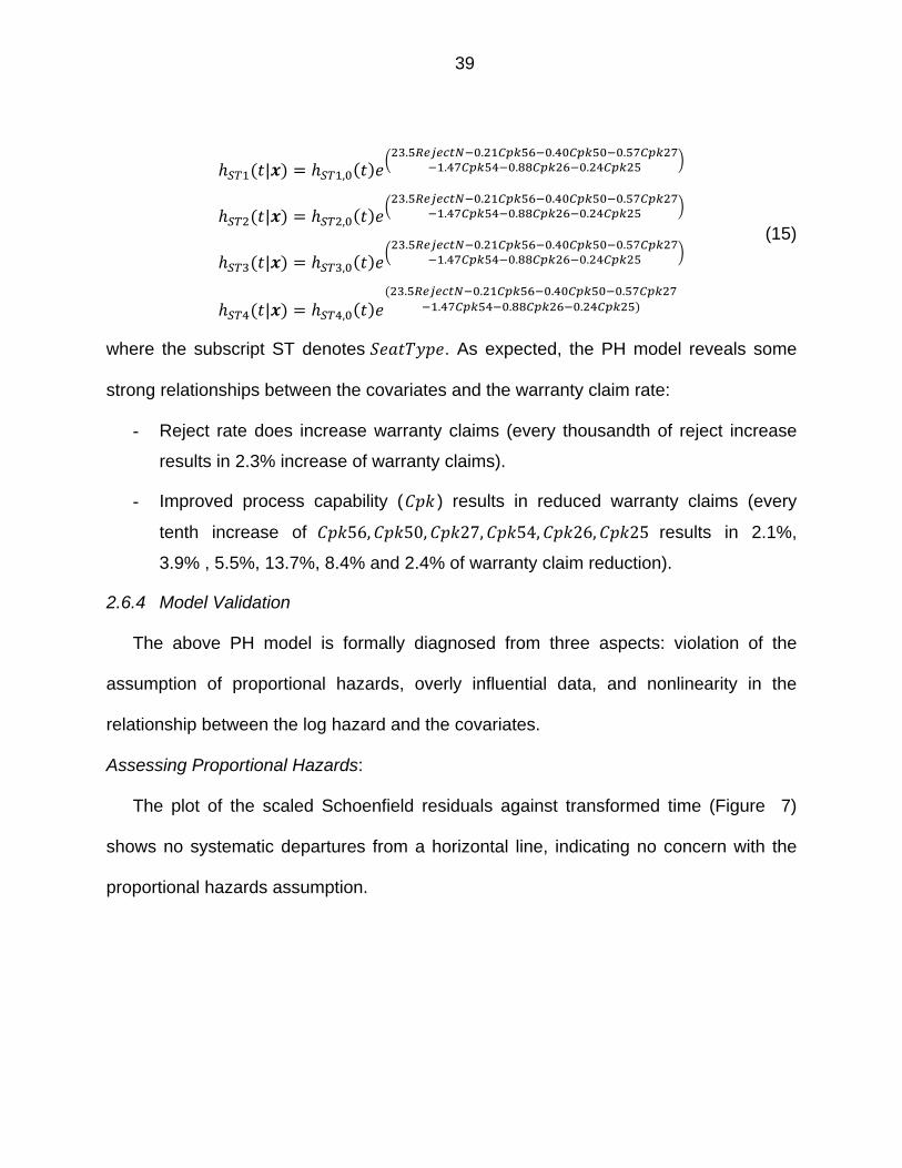
39

| ,

. . . .. . .

| ,

. . . .. . .

| ,

. . . .. . .

| ,

. . . .. . .

(15)

where the subscript ST denotes . As expected, the PH model reveals some

strong relationships between the covariates and the warranty claim rate:

- Reject rate does increase warranty claims (every thousandth of reject increase

results in 2.3% increase of warranty claims).

- Improved process capability ( ) results in reduced warranty claims (every

tenth increase of 56, 50, 27, 54, 26, 25 results in 2.1%,

3.9% , 5.5%, 13.7%, 8.4% and 2.4% of warranty claim reduction).

2.6.4 Model Validation

The above PH model is formally diagnosed from three aspects: violation of the

assumption of proportional hazards, overly influential data, and nonlinearity in the

relationship between the log hazard and the covariates.

Assessing Proportional Hazards:

The plot of the scaled Schoenfield residuals against transformed time (Figure 7)

shows no systematic departures from a horizontal line, indicating no concern with the

proportional hazards assumption.

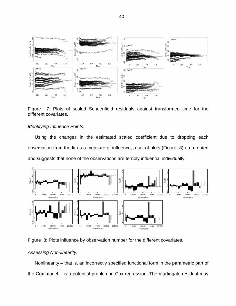
40

Figure 7: Plots of scaled Schoenfield residuals against transformed time for the different covariates.

Identifying Influence Points:

Using the changes in the estimated scaled coefficient due to dropping each

observation from the fit as a measure of influence, a set of plots (Figure 8) are created

and suggests that none of the observations are terribly influential individually.

Figure 8: Plots influence by observation number for the different covariates.

Assessing Non-linearity:

Nonlinearity – that is, an incorrectly specified functional form in the parametric part of

the Cox model – is a potential problem in Cox regression. The martingale residual may

Time

Bet

a(t)

for

Rej

ectN

110 260 400 530

-500

050

010

00

Time

Bet

a(t)

for

Cpk

56

110 260 400 530

-40

-20

010

Time

Bet

a(t)

for

Cpk

50

110 260 400 530

-15

-50

510

15

Time

Bet

a(t)

for

Cpk

27

110 260 400 530

-20

020

40

Time

Bet

a(t)

for

Cpk

54

110 260 400 530

-40

020

6010

0

Time

Bet

a(t)

for

Cpk

26

110 260 400 530

-20

020

4060

Time

Bet

a(t)

for

Cpk

25

110 260 400 530

-10

010

2030

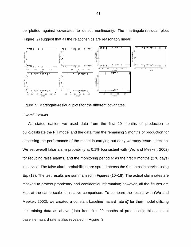
41

be plotted against covariates to detect nonlinearity. The martingale-residual plots

(Figure 9) suggest that all the relationships are reasonably linear.

Figure 9: Martingale-residual plots for the different covariates.

Overall Results

As stated earlier, we used data from the first 20 months of production to

build/calibrate the PH model and the data from the remaining 5 months of production for

assessing the performance of the model in carrying out early warranty issue detection.

We set overall false alarm probability at 0.1% (consistent with (Wu and Meeker, 2002)

for reducing false alarms) and the monitoring period as the first 9 months (270 days)

in service. The false alarm probabilities are spread across the 9 months in service using

Eq. (13). The test results are summarized in Figures (10~18). The actual claim rates are

masked to protect proprietary and confidential information; however, all the figures are

kept at the same scale for relative comparison. To compare the results with (Wu and

Meeker, 2002), we created a constant baseline hazard rate for their model utilizing

the training data as above (data from first 20 months of production); this constant

baseline hazard rate is also revealed in Figure 3.

RejectN

resi

d(fi

tRej

ectN

)

0.0 0.01 0.02 0.03

0.0

0.4

0.8

Cpk56

resi

d(fi

tCpk

56)

1.2 1.4 1.6 1.8 2.0

0.0

0.4

0.8

Cpk50

resi

d(fi

tCpk

50)

1.4 1.6 1.8 2.0 2.2 2.4 2.6

0.0

0.4

0.8

Cpk27

resi

d(fi

tCpk

27)

1.6 1.8 2.0 2.2 2.4 2.6

0.0

0.4

0.8

Cpk54

resi

d(fi

tCpk

54)

0.8 0.9 1.0 1.1 1.2 1.3 1.4

0.0

0.4

0.8

Cpk26

resi

d(fi

tCpk

26)

1.6 1.8 2.0 2.2 2.4 2.6

0.0

0.4

0.8

Cpk25re

sid(

fitC

pk25

)0.5 1.0 1.5 2.0

0.0

0.4

0.8

42

The plots from Figures (10~18) show that the PH model fit the training set quite well.

All the figures report the claims and their prediction limits for the different months in

production. The primary difference between the figures being the months in service

(different months have different production volumes, and hence, contribute to

estimation/variation in the prediction limits). It is readily apparent that the PH model

produces rather “tight” prediction limits for the claims across the different production

months (both for the training and testing datasets) as well as for the different months in

service. This is in significant contrast to the limits produced by Wu and Meeker’s

approach employing a constant baseline hazard rate function across all production

months. While the vehicles from the 24th month in production produced claims slightly

exceeding the PH model prediction limits during the seventh and ninth months in

service, they are not alarmingly outside the limits. Overall, it is clear from these plots

that the different covariates derived from the supply chain can greatly aid in improving

the accuracy of prediction limits, and in turn, enhance the detection power for early

detection of potential warranty issues. To be more conclusive, the proposed models

have to be further tested using warranty data sources from other systems, products,

and industries.

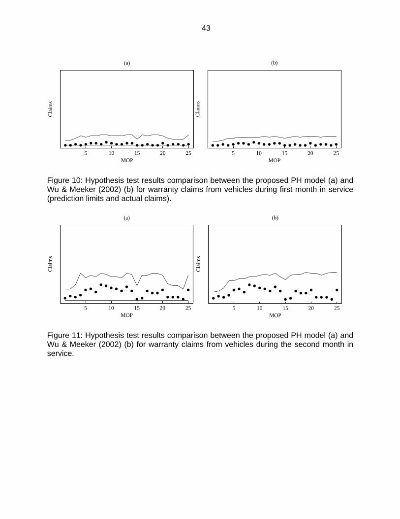
43

Figure 10: Hypothesis test results comparison between the proposed PH model (a) and Wu & Meeker (2002) (b) for warranty claims from vehicles during first month in service (prediction limits and actual claims).

Figure 11: Hypothesis test results comparison between the proposed PH model (a) and Wu & Meeker (2002) (b) for warranty claims from vehicles during the second month in service.

MOP

Cla

ims

5 10 15 20 25

(a)

MOP

Cla

ims

5 10 15 20 25

(b)

MOP

Cla

ims

5 10 15 20 25

(a)

MOP

Cla

ims

5 10 15 20 25

(b)

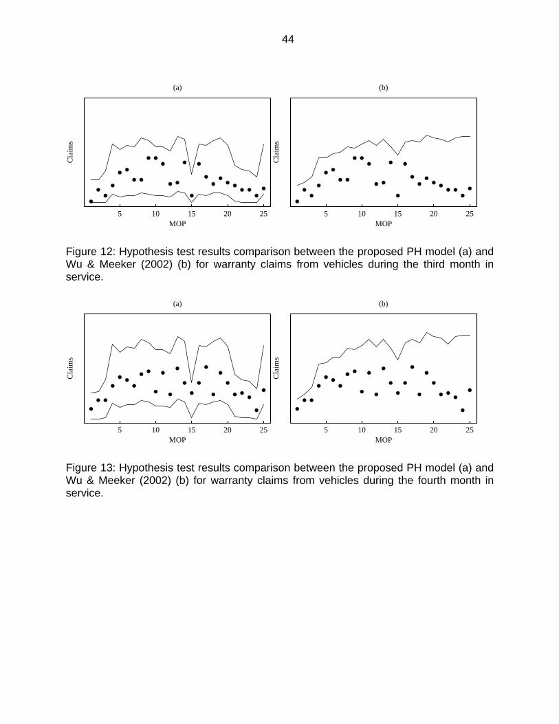
44

Figure 12: Hypothesis test results comparison between the proposed PH model (a) and Wu & Meeker (2002) (b) for warranty claims from vehicles during the third month in service.

Figure 13: Hypothesis test results comparison between the proposed PH model (a) and Wu & Meeker (2002) (b) for warranty claims from vehicles during the fourth month in service.

MOP

Cla

ims

5 10 15 20 25

(a)

MOP

Cla

ims

5 10 15 20 25

(b)

MOP

Cla

ims

5 10 15 20 25

(a)

MOP

Cla

ims

5 10 15 20 25

(b)

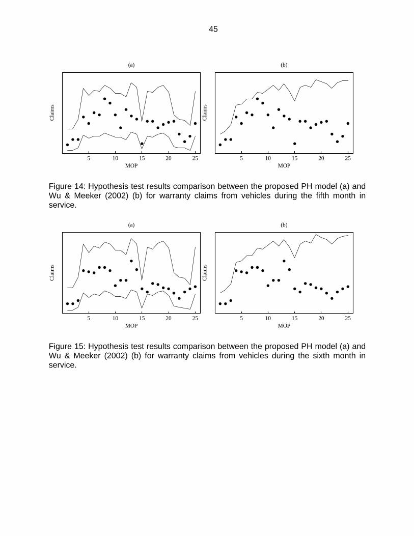
45

Figure 14: Hypothesis test results comparison between the proposed PH model (a) and Wu & Meeker (2002) (b) for warranty claims from vehicles during the fifth month in service.

Figure 15: Hypothesis test results comparison between the proposed PH model (a) and Wu & Meeker (2002) (b) for warranty claims from vehicles during the sixth month in service.

MOP

Cla

ims

5 10 15 20 25

(a)

MOP

Cla

ims

5 10 15 20 25

(b)

MOP

Cla

ims

5 10 15 20 25

(a)

MOP

Cla

ims

5 10 15 20 25

(b)

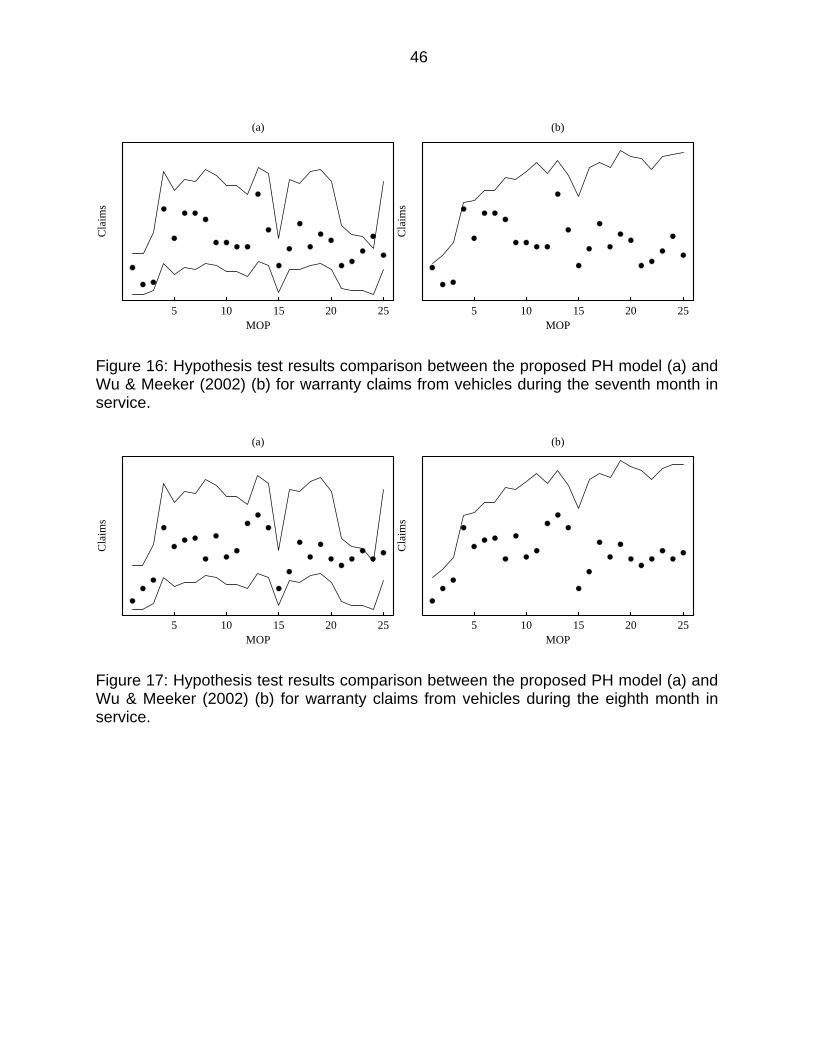
46

Figure 16: Hypothesis test results comparison between the proposed PH model (a) and Wu & Meeker (2002) (b) for warranty claims from vehicles during the seventh month in service.

Figure 17: Hypothesis test results comparison between the proposed PH model (a) and Wu & Meeker (2002) (b) for warranty claims from vehicles during the eighth month in service.

MOP

Cla

ims

5 10 15 20 25

(a)

MOP

Cla

ims

5 10 15 20 25

(b)

MOP

Cla

ims

5 10 15 20 25

(a)

MOP

Cla

ims

5 10 15 20 25

(b)

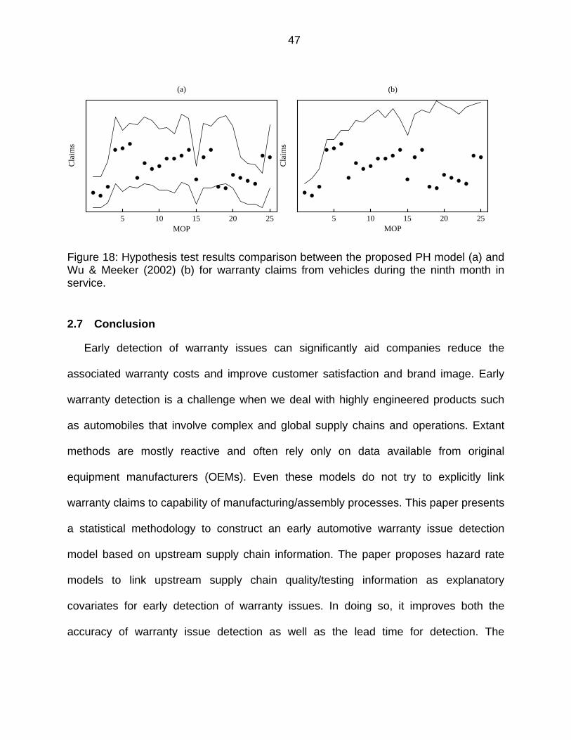
47

Figure 18: Hypothesis test results comparison between the proposed PH model (a) and Wu & Meeker (2002) (b) for warranty claims from vehicles during the ninth month in service.

2.7 Conclusion

Early detection of warranty issues can significantly aid companies reduce the

associated warranty costs and improve customer satisfaction and brand image. Early

warranty detection is a challenge when we deal with highly engineered products such

as automobiles that involve complex and global supply chains and operations. Extant

methods are mostly reactive and often rely only on data available from original

equipment manufacturers (OEMs). Even these models do not try to explicitly link

warranty claims to capability of manufacturing/assembly processes. This paper presents

a statistical methodology to construct an early automotive warranty issue detection

model based on upstream supply chain information. The paper proposes hazard rate

models to link upstream supply chain quality/testing information as explanatory

covariates for early detection of warranty issues. In doing so, it improves both the

accuracy of warranty issue detection as well as the lead time for detection. The

MOP

Cla

ims

5 10 15 20 25

(a)

MOP

Cla

ims

5 10 15 20 25

(b)

48

proposed methodology is illustrated and validated using real-world data from a leading

Tier-1 automotive supplier.

There is other upstream supply chain information related major design/process

change with which little to no warranty historical warranty claim data exists to associate,

to link this type of information to warranty claims, the next chapter extend the proposed

models to account for the warranty claim judgments of subject matter experts (e.g.,

opinions of design, process, quality and testing experts regarding design/process

changes) and information from Tier-2 and further upstream suppliers. Suppliers that

supply systems for multiple OEMs should also be able to exploit warranty claims

information from multiple OEM customers.

49

CHAPTER 3 BAYESIAN APPROACH TO HAZARD RATE MODELS FOR EARLY WARRANTY ISSUES DETECTION

3.1 Introduction

In the previous chapter, we utilized upstream supply chain information such as

product reject rate from end-of-line tests and manufacturing process capability in the

form of covariates for hazard rate models to detect early on warranty issues and predict

future warranty claims. The upstream supply chain information exploited is mostly from

routine manufacturing process and historical data from the plant and observed warranty

claims were used to build and calibrate the hazard rate models. However, as is evident

from Figure 1, there are a number of other upstream supply chain data sources that can

aid the development of effective warranty issue detection models. In particular,

information from product development, major design change/upgrade efforts,

manufacturing technology upgrades etc. This type of information might initially be

available only in the form of results from prototype/bench tests and judgments from

subject-matter-experts (SMEs) but there might be little to no warranty historical data to

recalibrate the models to account for the changes. Here are some example scenarios:

After product is launched, incoming warranty claims exhibit excessive design

related fatigue failure due to certain customer usage patterns not being captured

in verification tests during the product design phase. Once such warranty issue is

realized, a design change is quickly implemented to address the issue.

Due to process technology improvements, suppliers may make a major

manufacturing process change (e.g., switch from gas metal arc welding to laser

beam welding).

50

An existing supplier's subsystem such as seat with warranty claim history will

supplied to different vehicle models for the same or a new OEM.

Suppliers add new features to their subsystem per OEM's request to meet

consumers' rapidly evolving demand.

Under these types of scenarios, the management might hope to know the impact of

such major changes on warranty performance early on so that any necessary counter

measures can be quickly implemented to reduce risks. Unfortunately, we cannot blindly

wait for the claims patterns/rates to be revealed from the field.

Suppliers often have some information for process/design and application changes.

For examples, for a design related fatigue failure, suppliers may have run accelerated

lab test for existing design and new design under newly realized customer usage

patterns; for a major process change, such as a welding process change, suppliers may

have information from production trials in the plant to evaluate scarp rate; for cases

involving an existing subsystem being newly employed in other product models or with

new features, suppliers may have extensive design verification results under the new

applications. Also, suppliers often have good expert knowledge and opinion on the

effects of the above changes from SMEs.

Unfortunately the above upstream supply chain information cannot be directly

applied to hazard rate models for there is often no good field warranty claims data

directly associated with it. We aim here to extend the hazard rate models proposed in

Chapter 2 to exploit judgments of SMEs regarding the changes and information

available from testing efforts (e.g., bench tests) to facilitate earlier and improved

detection of warranty issues/improvements from the changes.

51

3.2 Bayesian Approach to Encapsulate Upstream Supply Chain Information

Let us revisit the proportional hazard (PH) model for warranty issue detection from

the previous chapter:

| exp (16)

where denotes the baseline (warranty claim) hazard rate and the set of

covariates (e.g., quality measured by end-of-line tests and process capability of different

processes). We now adapt this model to account for the impact of design and/or

process changes on warranty claims.

now denotes the vector of binary covariates indicating the different

design/process/application changes and the regression coefficients for the same.

Previously, we adopted the frequentist approach of the likelihood method and purely

relied on historical warranty claims data to estimate the model coefficients. However, as

stated earlier, in the presence of major design changes, we cannot afford to wait for the

warranty claims patterns/rates to be revealed from the field. Instead, we adopt a

Bayesian approach to exploit priors available based on the judgments of SMEs and

bench tests/plant trials. We hypothesize that this extended Bayesian hazard rate model

provides the potential to reduce warranty issue detection time with more power. It is

however extremely important that the priors be reliable and accurate in terms of bias

and precision, the construction of which can be quite involved. Guidelines for the same

are provided in sections to follow.

More importantly, Bayesian method provides us a precise prescription to

refine/update our prior distributions sequentially, as new warranty claims (associated

with major design/process/application changes) get revealed over time from the field.

52

Based on the Bayes' theorem, the posterior distribution is proportional to the product of

the conditional likelihood of the new warranty claims and the prior distribution for . The

posteriors derived using data from the first monitoring period will form the updated priors

for the second monitoring period and so on. After each sequential monitoring period,

will be closer to the true value with reduced variances, the estimated impact for the

changes will be closer to true impact. Accurate prior distributions based on upstream

supply chain information will make the subsequent posterior distributions converge

faster to true , so that it can reduce warranty detection time with more power.

Since Bayesian inference is introduced (Lindley and Smith, 1972) it has been

applied in reliability (Singpurwalla, 1988b), with an extensive review from a Bayesian

perspective (Singpurwalla, 1988a, 2006). Bayesian analysis was also extended to

proportional hazard model due to its popularity of being easy to interpret and well

understood in engineering community.

Bayesian analysis was applied to proportional hazard model in two aspects: non-

parametric and parametric. On the one hand, regression coefficient vector of covariates

is always assumed to have prior distributions with possibly unknown hyperparameters,

on the other hand, the baseline hazard function can be treated non-parametrically

as in semi-parametric proportional hazard model (Cox, 1972), or parametrically as

Weibull or extreme value distribution. Therefore its prior distributions have to be

specified non-parametrically or parametrically accordingly.

The idea to handle the prior distribution of non-parametrically is first to

discretize in the form of piecewise constant, non-decreasing jump etc, then apply

stochastic processes which have a convenient property of conjugacy. The prior

53

distribution can be treated as the realization of such stochastic processes. Several such

stochastic processes have been proposed starting from Dirichlet processes on survival

function (Ferguson, 1973), then neutral to the right (NTR) processes on survival function

which overcomes limitation of Dirichlet process of being losing its property of conjugacy

under right censoring (Doksum, 1974) and left truncation (Kim and Lee, 2003), then

followed by gamma process (Kalbfleisch, 1978), beta process (Hjort, 1990) and random

finite-mixture process (Gelfand and Mallick, 1995) on cumulative hazard function. The

pros and cons for above methods have been extensively reviewed (Sinha and Dey,

1997; Singpurwalla, 2006).

The prior distribution of can also be handled parametrically by fitting it to

known parametric proportional hazards model such as Weibull and the extreme value

model (Kim and Ibrahim, 2000; Zuashkiani et al., 2006)

But obtaining the posterior distribution is computationally challenging. Conjugate

priors are convenient ways to obtain the closed form of posterior without computation

burden. However conjugate priors are exception instead of rule in Bayesian analysis.

Even for the simple and popular Weibull distribution without covariate, its posterior is not

analytical tractable due to involving the integral of a non-linear function of the

parameters; numerical integration and Monte Carlo simulation has to be resorted

(Tsokos and Canavos, 1972; Canavos and Tsokos, 1973). Generally obtaining

Bayesian posterior for hazard rate model is daunting and becomes a road block for

implementation of Bayesian approach to hazard rate model. It triggers researchers to

resort computation intensive numerical approach by taking advantage of modern

computer power. This approach ranges from simple Monte Carlo sampling (Smith and

54

Gelfand, 1992) to more advanced Markov chain Monte Carlo (MCMC) algorithms such

as data augmentation, Gibbs sampling, and sampling-importance-resampling (Gelfand

and Smith, 1990; Gelfand and Mallick, 1995). Since MCMC is easily to be coded into

computer program, it emerges as a standard procedure in statistical software to attack

common computation problems encountered in Bayesian analysis.

In the following sections, we will tailor above Bayesian analysis methods to our early

warranty detection scheme, so that base on the unique property of warranty claims with

upstream supply chain information, we can implemented Bayesian analysis to hazard

rate model in a practical way with computation efficiency.

3.3 Statistical Framework to Obtain Posterior Distribution of Hazard Rate Model

To fully examine the hazard rate model of Eq. (16) from a Bayesian prospective, we

need priors for both the baseline hazard rate (i.e., ) as well as the proportional

model regression coefficient vector (i.e., ). This is rather demanding for constructing

priors for in the absence of good historical data is rather challenging. One could

partially overcome this difficulty by adopting a parametric PH model with the baseline

hazard following a standard distribution (e.g., Weibull or Gamma). However, given that

design and process/technology changes are made to existing products and processes,

respectively, assuming that the impact of the change is proportional to the earlier

hazard rate, we can utilize the baseline hazard rate function established from historical

data for the earlier product. We adopt this approach throughout this chapter (i.e.,

is known). Future work will account for to be an unknown random variable or know

with some uncertainty.

55

Overall, we divide the covariates into two groups:

– covariates employed by the PH model calibrated using historical data for the

previous product (i.e., before the product/process underwent major changes),

denoted by with coefficients denoted by

– second group constitutes the binary covariates representative of the major

changes, denoted by with coefficients denoted by

As stated earlier, the Bayesian analysis will only be applied to . The proposed

Bayesian approach to extend the hazard rate model is formally defined as:

(17)

~ (18)

Suppose , are 1 vectors , , … , ′ and , , … , ′ .

1,2,… , is coded as a binary covariate with 0 if it is an existing

design/process/application and with 1 if it is new design/process/application.

1,2, … , denotes the associated regression coefficient to quantify the relative

hazard rate impact. Each is assigned a prior distribution of .

We assume that is independent of and will not change the baseline hazard

function. Also, we assume that is independent of .

Based on the Bayes' law (Singpurwalla, 2006), the posterior distributions after

independent warranty claims , , , , , , … , , , are observed during

the 1st monitoring period are:

56

, , , , , , … , , ,

, , , , , , … , , ,, , , , , , … , , , |

(19)

where is the censored th unit service age with corresponding changes as covariate

vectors . The indicator variable 1 if the th unit experienced a warranty claim for

the subsystem of interest at service age ; 0 if the th unit has not produced any

warranty claim until age .

, , , , , , … , , , is the likelihood of given the

warranty claims , , , , , , … , , , . This likelihood can be estimated

as:

, , , , , , … , , ,

(20)

Since , , are all known, ∏ is a

constant, set it as , then:

, , , , , , … , , , (21)

57

∑ ∑

Set 1,2,… , . Also, given that ∏ is known and is a

constant, set ∏ . Then:

, , , , , , … , , ,

∑ ∑ ∏

(22)

Here, , , … , . The posterior distribution of can then be

expressed as:

, , , , , , … , , ,

∏∑ ∑ ∏

∏∑ ∑ ∏

∏∑ ∑ ∏

∏∑ ∑ ∏

(23)

58

When there is only one design/process/application change (i.e., 1), and

. The likelihood function can then be simplified as:

, , , , , , … , , , |

∑ ∑

∑ ∑ ∑

∑ ∑ ∑

(24)

Here, denotes the number of units fielded prior to the change (i.e., data

corresponding to 0). denotes the number of units fielded post change. We

denote . Setting ∑ , ∑ , ∑ , which

are all constants, we have:

, , , , , , … , , , |

(25)

The posterior distribution can then be simplified as:

| , , , , , , … , , ,

(26)

Obviously, if the prior distribution of is a gamma distribution:

~ , (27)

Its posterior distribution is also a gamma distribution:

| , , , , , , … , , ,

Γ~ ,

(28)

59

where ∑ and ∑ . It is interesting to note that is the warranty

claims associated with the change (i.e., the new design/process/application), is the

sum of the cumulative hazard rates for units under the new design/process/application.

The additional new warranty claims for units with existing design/process/application will

not shed any light on the posterior distribution of .

When there are two or more design/process/application changes, multiple covariates

will be necessary. Then, in the exponent of the last item of Eq.(22) are compounded

and cannot be separated; the closed-form of 's posterior does not exist, numerical

Bayesian methods have to be pursued (see (Gelfand and Smith, 1990) for further

information on numerical Bayesian methods).

We propose two numerical Bayesian methods to obtain 's posteriors when more

than one change is involved. The first method is a non-parametric method whereas the

second is a parametric method.

3.3.1 Large Sample Size Bayesian Analysis

Here, we adopt the large sample Bayesian analysis from (Faraggi and Simon, 1997).

In the PH model shown in Eq.(16), since their interest focus on estimation of regression

coefficients rather than on prediction of the survival function, they avoided placing a

prior distribution on to derive the posterior distribution. Instead, they only assigned

a multivariate Gaussian prior to , then obtained the large sample approximation of

posterior | via MLE using the standard Cox procedure (Cox, 1972). This method was

adopted in our application as the following procedure:

60

1. Estimate Baseline PH Model: Use historical warranty claims with upstream

supply chain information to estimate and in Eq.(17) by maximizing

Cox’s partial log-likelihood:

′ (29)

where is the number of units from the existing design/process/application for

which there exists a partial or full warranty claim history, variable , called the

risk indicator, equals 1 if and only if the th unit has no warranty claim and is still

in service at time , and hence, at risk of generating a claim at time . Hence,

and become known variables.

2. Assign Prior: When the new design/process/application changes have been

implemented into suppliers' subsystems, assign with a Gaussian prior

, Σ from upstream supplier chain information where is

1 mean vector, Σ is variance matrix. Start monitoring warranty claims

from units associated with these new design/process/application changes.

3. MLE: During the first monitoring period, suppose there are units with both

existing design/process/application and new design/process/application for which

there exists a partial or full warranty claim history, we estimate as in (17)

by maximizing Cox’s partial log-likelihood as follows:

′ log (30)

61

Under large sample size, the probability density function of can be

approximated by a Gaussian distribution:

~ , (31)

where is the observed information matrix, which can be estimated as:

(32)

4. Derive Posterior: During the first monitoring period, the posterior distribution of

can be evaluated based on :

|

∝ , , Σ

(33)

The above posterior is proved to be Gaussian (Lindley and Smith, 1972):

| , Σ

Σ Σ

Σ Σ

(34)

It is easy to see that the Bayes estimator for is a weighted average of the

MLE and the mean of the prior . When is a scalar variable with

~ , σ , then the Bayes estimator for is the familiar form of

posterior for Gaussian conjugate prior with known variance.

σ

σ σ

σσ

σ

(35)

62

5. Update and : update and per step 1 based on new incoming

warranty claims from existing design/process/application during the first

monitoring period. When the warranty claims for existing

design/process/application are fully mature, and will change little; when

the warranty claims for existing design/process/application are not fully mature

especially in high time in service, this updating can improve the accuracy of the

model by iterative calibration per monitoring period.

6. Use Old Posterior as New Prior: During the second monitoring period, suppose

there are units with both existing design/process/application and new

design/process/application for which there exists a partial or full warranty claim

history, replace the prior of with its posterior , Σ from the first

monitoring period; estimate MLE from Eq.(30) based on ; and then obtain

the 's posterior , Σ .

7. Repeat: Repeat steps 2-6 for each monitoring period.

For monitoring periods, 1 sequence of posteriors of will be obtained as

, Σ , , Σ , … , , Σ . It was shown (Faraggi and Simon, 1997)

that such a Bayesian estimation process has superior performance over using Cox

model directly without Bayesian treatment.

The advantage of the large sample size method is computational efficiency; eases

burden of computing posterior of . The difficulty with the method proposed by

(Faraggi and Simon, 1997) is that they lack prior knowledge of . Hence, the

63

survival function cannot be predicted. In our case, we overcome that difficulty because

of availability of historical claims data from the existing design/process/application to

estimate accurately (as discussed in Step-1 above). The only assumption made is

that MLE is approximately normal, valid under large sample sizes. (Faraggi and

Simon, 1997) showed that when the ratio of the number of events (warranty claims in

our case) to the number of covariates is larger than 15, the approximation is accurate.

In our case, large sample size is the unique property of warranty claims due to large

population of units in the field (in particular, for automotive industry). The

implementation of this procedure is easy as standard modules are available in most

statistical software to estimate MLE , and the posterior of can be computed

without special software due to the convenient properties of the Gaussian distribution.

3.3.2 Monte Carlo Markov Chain (MCMC) Bayesian Analysis

In the parametric method, we assume warranty claims follow a Weibull distribution

with shape parameter 0 and scale parameter 0:

(36)

We assume that only the scale parameter depends on covariates :

(37)

From Eq.(37), Eq.(36) takes the parametric form of Eq.(16):

(38)

with as the baseline hazard function. Dividing into and as

before, Eq.(39) takes the parametric form of Eq.(17):

(39)

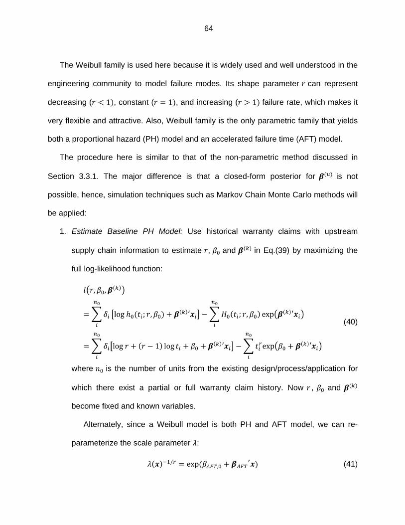
64

The Weibull family is used here because it is widely used and well understood in the

engineering community to model failure modes. Its shape parameter can represent

decreasing ( 1 , constant ( 1 , and increasing ( 1 failure rate, which makes it

very flexible and attractive. Also, Weibull family is the only parametric family that yields

both a proportional hazard (PH) model and an accelerated failure time (AFT) model.

The procedure here is similar to that of the non-parametric method discussed in

Section 3.3.1. The major difference is that a closed-form posterior for is not

possible, hence, simulation techniques such as Markov Chain Monte Carlo methods will

be applied:

1. Estimate Baseline PH Model: Use historical warranty claims with upstream

supply chain information to estimate , and in Eq.(39) by maximizing the

full log-likelihood function:

, ,

log ; , ′ ; , exp ′

log 1 log ′ exp ′

(40)

where is the number of units from the existing design/process/application for

which there exist a partial or full warranty claim history. Now , and

become fixed and known variables.

Alternately, since a Weibull model is both PH and AFT model, we can re-

parameterize the scale parameter :

/ exp , (41)

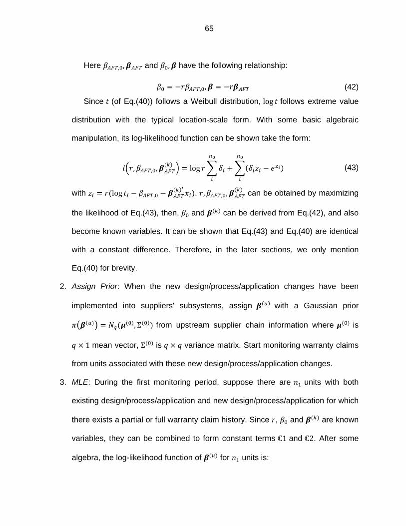
65

Here , , and , have the following relationship:

, , (42)

Since (of Eq.(40)) follows a Weibull distribution, log follows extreme value

distribution with the typical location-scale form. With some basic algebraic

manipulation, its log-likelihood function can be shown take the form:

, , , log (43)

with log , . , , , can be obtained by maximizing

the likelihood of Eq.(43), then, and can be derived from Eq.(42), and also

become known variables. It can be shown that Eq.(43) and Eq.(40) are identical

with a constant difference. Therefore, in the later sections, we only mention

Eq.(40) for brevity.

2. Assign Prior: When the new design/process/application changes have been

implemented into suppliers' subsystems, assign with a Gaussian prior

, Σ from upstream supplier chain information where is

1 mean vector, Σ is variance matrix. Start monitoring warranty claims

from units associated with these new design/process/application changes.

3. MLE: During the first monitoring period, suppose there are units with both

existing design/process/application and new design/process/application for which

there exists a partial or full warranty claim history. Since , and are known

variables, they can be combined to form constant terms 1 and 2. After some

algebra, the log-likelihood function of for units is:

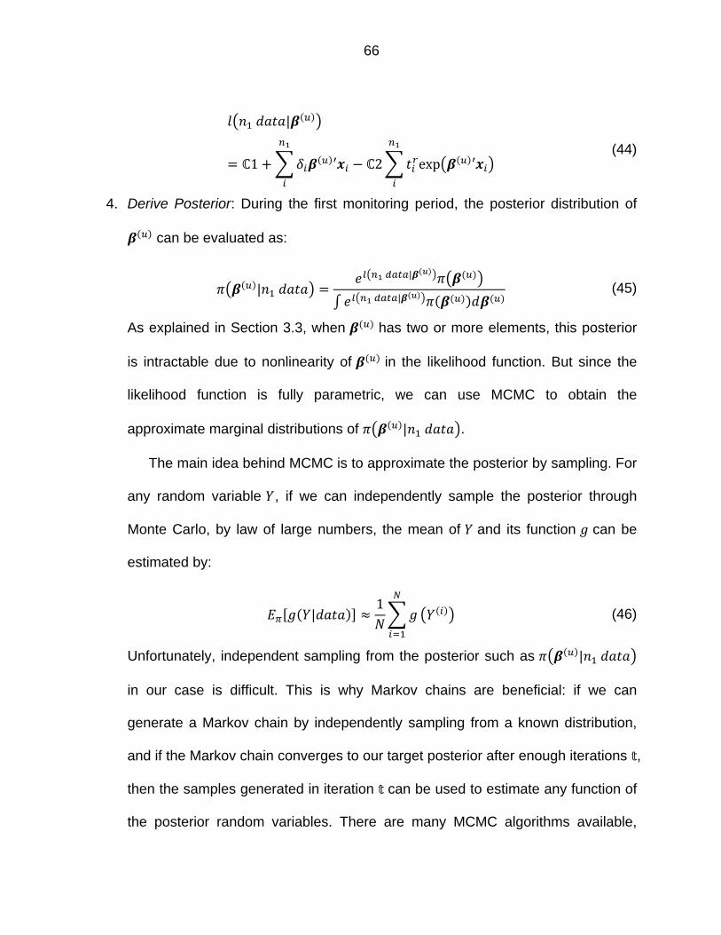
66

|

1 ′ 2 exp ′ (44)

4. Derive Posterior: During the first monitoring period, the posterior distribution of

can be evaluated as:

| |

| (45)

As explained in Section 3.3, when has two or more elements, this posterior

is intractable due to nonlinearity of in the likelihood function. But since the

likelihood function is fully parametric, we can use MCMC to obtain the

approximate marginal distributions of | .

The main idea behind MCMC is to approximate the posterior by sampling. For

any random variable , if we can independently sample the posterior through

Monte Carlo, by law of large numbers, the mean of and its function can be

estimated by:

|1

(46)

Unfortunately, independent sampling from the posterior such as |

in our case is difficult. This is why Markov chains are beneficial: if we can

generate a Markov chain by independently sampling from a known distribution,

and if the Markov chain converges to our target posterior after enough iterations ,

then the samples generated in iteration can be used to estimate any function of

the posterior random variables. There are many MCMC algorithms available,

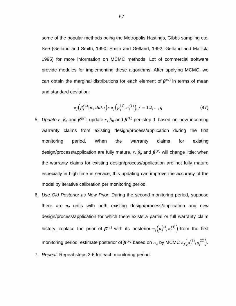
67

some of the popular methods being the Metropolis-Hastings, Gibbs sampling etc.

See (Gelfand and Smith, 1990; Smith and Gelfand, 1992; Gelfand and Mallick,

1995) for more information on MCMC methods. Lot of commercial software

provide modules for implementing these algorithms. After applying MCMC, we

can obtain the marginal distributions for each element of in terms of mean

and standard deviation:

| ~ , ; 1,2, … , (47)

5. Update , and : update , and per step 1 based on new incoming

warranty claims from existing design/process/application during the first

monitoring period. When the warranty claims for existing

design/process/application are fully mature, , and will change little; when

the warranty claims for existing design/process/application are not fully mature

especially in high time in service, this updating can improve the accuracy of the

model by iterative calibration per monitoring period.

6. Use Old Posterior as New Prior: During the second monitoring period, suppose

there are untis with both existing design/process/application and new

design/process/application for which there exists a partial or full warranty claim

history, replace the prior of with its posterior , from the first

monitoring period; estimate posterior of based on by MCMC , .

7. Repeat: Repeat steps 2-6 for each monitoring period.

68

3.4 Constructing Prior for

The performance of all Bayesian methods rely on the quality of the priors. Accurate

construction of the prior plays a key role for early warranty detection; a strong

but correct prior can lead us toward the right direction earlier with more power.

Constructing a prior is essentially the effort to abstract upstream supply chain

information in a probability form with a few hyper-parameters.

Priors can come from two approaches: objective approach by exploring empirical

data and subjective approach by subject matter expert (SME) judgment. Unlike some

situations such as early development phase, objective data is scarce, and subjective

approach is the only source. When it comes down to warranty issue detection, it is

already in the late development phase and lab tests and production trial results can be

available. So for warranty detection, our recommended strategy is to use expert

judgment as a complement of empirical data: first get the initial uncertainty

quantification of by exploring empirical data from lab tests and production trials, and

fine tune the uncertainty using SME judgment.

Since not all SMEs are trained and think in terms of probability, prior has to be

transformed into SME’s natural language. A nice feature of the hazard rate model is the

relatively easy interpretation of in terms of hazard rate, which is a familiar concept

in reliability engineering and well understood by SMEs. As the covariates are binary

indicators represents existing design/process/application and

represents the major design/process/application change), the impact of such changes

can be easily interpreted by relative hazard rate increase or decrease and readily

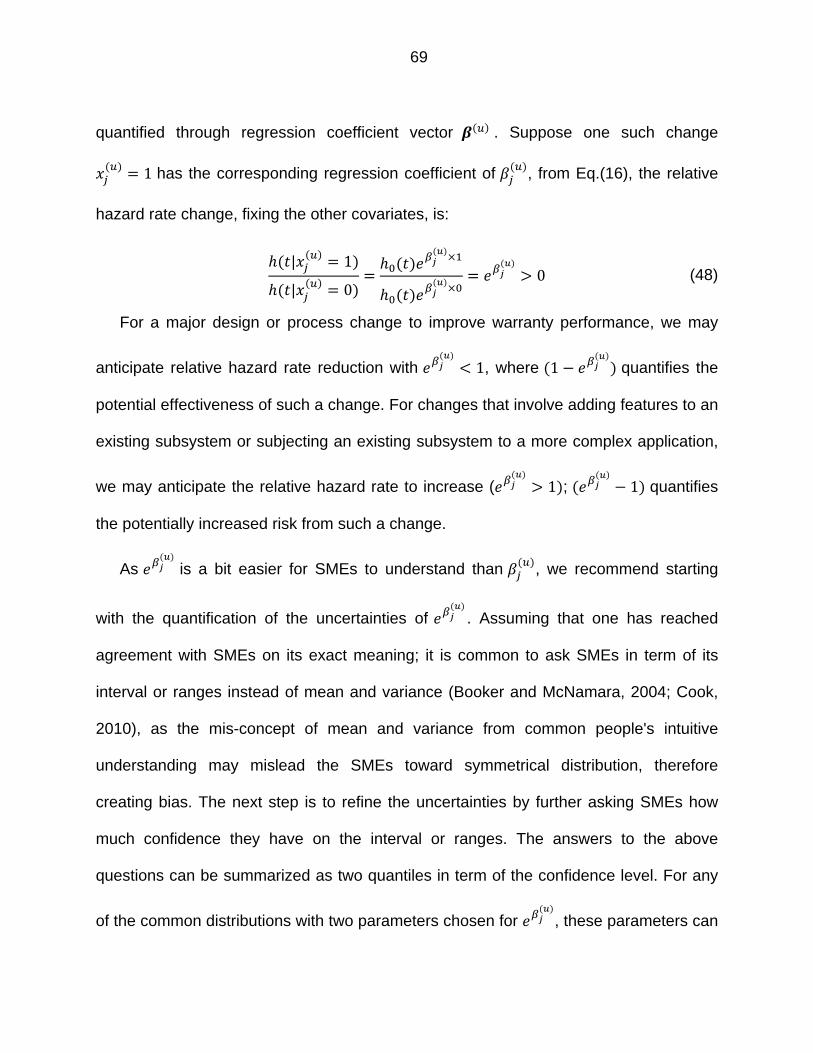
69

quantified through regression coefficient vector . Suppose one such change

1 has the corresponding regression coefficient of , from Eq.(16), the relative

hazard rate change, fixing the other covariates, is:

| 1

| 00 (48)

For a major design or process change to improve warranty performance, we may

anticipate relative hazard rate reduction with 1, where 1 quantifies the

potential effectiveness of such a change. For changes that involve adding features to an

existing subsystem or subjecting an existing subsystem to a more complex application,

we may anticipate the relative hazard rate to increase ( 1 ; 1 quantifies

the potentially increased risk from such a change.

As is a bit easier for SMEs to understand than , we recommend starting

with the quantification of the uncertainties of . Assuming that one has reached

agreement with SMEs on its exact meaning; it is common to ask SMEs in term of its

interval or ranges instead of mean and variance (Booker and McNamara, 2004; Cook,

2010), as the mis-concept of mean and variance from common people's intuitive

understanding may mislead the SMEs toward symmetrical distribution, therefore

creating bias. The next step is to refine the uncertainties by further asking SMEs how

much confidence they have on the interval or ranges. The answers to the above

questions can be summarized as two quantiles in term of the confidence level. For any

of the common distributions with two parameters chosen for , these parameters can

70

be fully defined (Cook, 2010). The prior distribution for can then be obtained by

transforming from to .

In reality, the elicitation process can be complicated due to many human factors

such as cognition, psychology involved during the process of interpreting diverse data,

knowledge, and experience. Fortunately there are many techniques (Cooke, 1994) and

tools (Booker et al., 2003) available. For example, if SMEs can only quantify the

effectiveness of a design/process improvement in terms of scales 1 to 10, or in a natural

language of excellent, good, average, poor, unacceptable, the method to link fuzzy set

theory and probability can be used (Booker and Singpurwalla, 2003; Yadav et al., 2003).

The choice of prior distribution form for is more commonly based on

mathematical convenience instead of physical justification. The common choice for

is Gaussian due to its well known properties, so is a lognormal distribution.

Sometimes, a gamma distribution is chosen for for its conjugate properties.

(Clemen et al., 1996) show that a Gaussian prior offers the same level of performance

as other complex models. The choice of prior distribution does not pose a serious

limitation as there is rarely sufficient prior information to differentiate the difference.

To minimize the bias generated from expert judgments, we select multiple SMEs

from diverse backgrounds. SMEs can be design/process engineers who create the

design/process changes, quality and production engineers who work on the production

lines, test engineers who test the design change, etc. From elicitation process, one prior

probability distribution is generated from each expert. The multiple prior probability

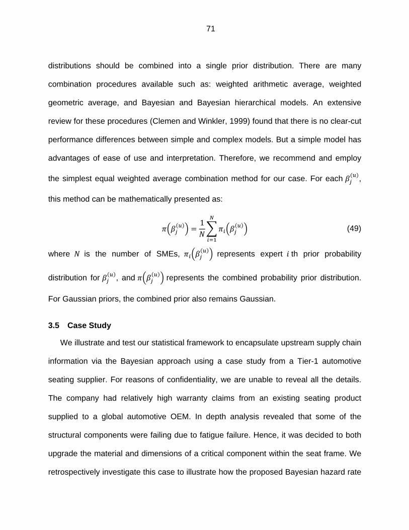
71

distributions should be combined into a single prior distribution. There are many

combination procedures available such as: weighted arithmetic average, weighted

geometric average, and Bayesian and Bayesian hierarchical models. An extensive

review for these procedures (Clemen and Winkler, 1999) found that there is no clear-cut

performance differences between simple and complex models. But a simple model has

advantages of ease of use and interpretation. Therefore, we recommend and employ

the simplest equal weighted average combination method for our case. For each ,

this method can be mathematically presented as:

1 (49)

where is the number of SMEs, represents expert th prior probability

distribution for , and represents the combined probability prior distribution.

For Gaussian priors, the combined prior also remains Gaussian.

3.5 Case Study

We illustrate and test our statistical framework to encapsulate upstream supply chain

information via the Bayesian approach using a case study from a Tier-1 automotive

seating supplier. For reasons of confidentiality, we are unable to reveal all the details.

The company had relatively high warranty claims from an existing seating product

supplied to a global automotive OEM. In depth analysis revealed that some of the

structural components were failing due to fatigue failure. Hence, it was decided to both

upgrade the material and dimensions of a critical component within the seat frame. We

retrospectively investigate this case to illustrate how the proposed Bayesian hazard rate

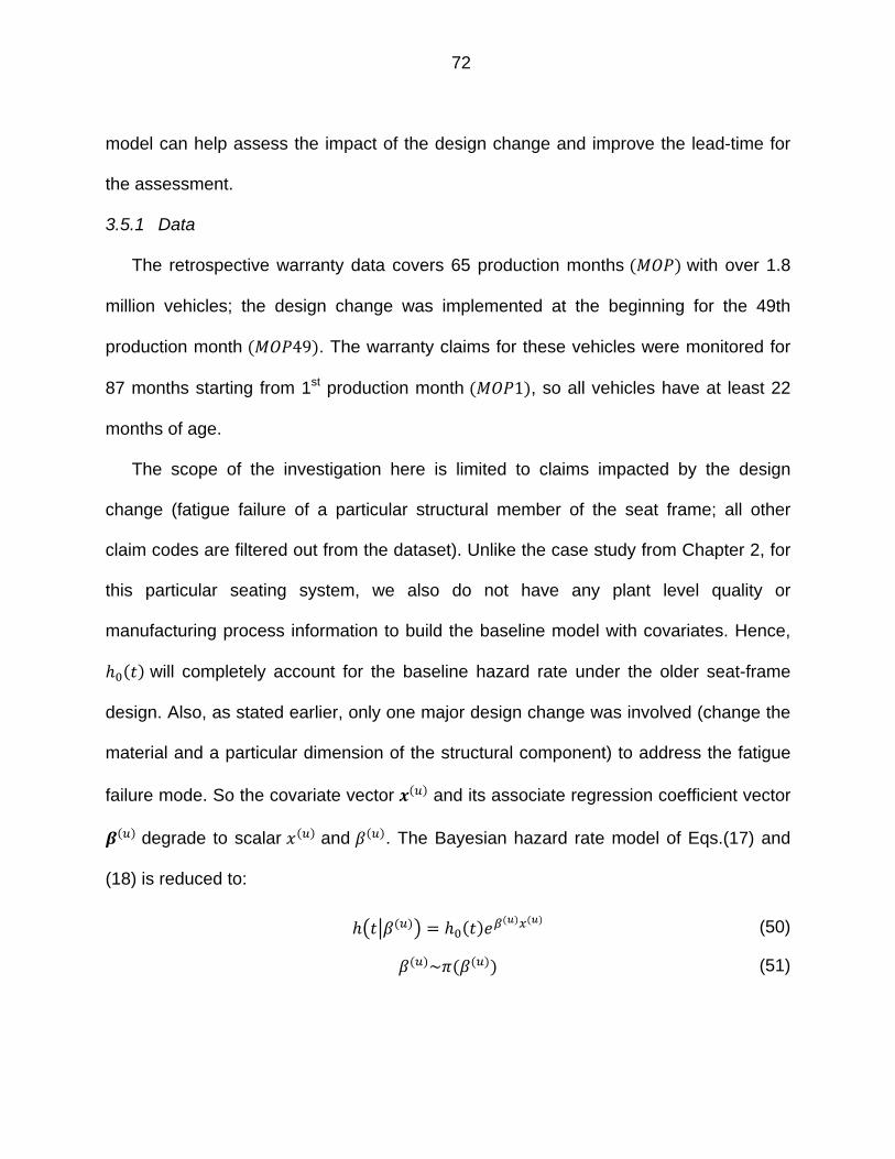
72

model can help assess the impact of the design change and improve the lead-time for

the assessment.

3.5.1 Data

The retrospective warranty data covers 65 production months with over 1.8

million vehicles; the design change was implemented at the beginning for the 49th

production month 49 . The warranty claims for these vehicles were monitored for

87 months starting from 1st production month 1 , so all vehicles have at least 22

months of age.

The scope of the investigation here is limited to claims impacted by the design

change (fatigue failure of a particular structural member of the seat frame; all other

claim codes are filtered out from the dataset). Unlike the case study from Chapter 2, for

this particular seating system, we also do not have any plant level quality or

manufacturing process information to build the baseline model with covariates. Hence,

will completely account for the baseline hazard rate under the older seat-frame

design. Also, as stated earlier, only one major design change was involved (change the

material and a particular dimension of the structural component) to address the fatigue

failure mode. So the covariate vector and its associate regression coefficient vector

degrade to scalar and . The Bayesian hazard rate model of Eqs.(17) and

(18) is reduced to:

(50)

~ (51)

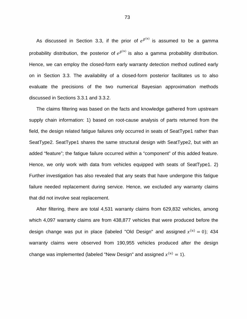
73

As discussed in Section 3.3, if the prior of is assumed to be a gamma

probability distribution, the posterior of is also a gamma probability distribution.

Hence, we can employ the closed-form early warranty detection method outlined early

on in Section 3.3. The availability of a closed-form posterior facilitates us to also

evaluate the precisions of the two numerical Bayesian approximation methods

discussed in Sections 3.3.1 and 3.3.2.

The claims filtering was based on the facts and knowledge gathered from upstream

supply chain information: 1) based on root-cause analysis of parts returned from the

field, the design related fatigue failures only occurred in seats of SeatType1 rather than

SeatType2. SeatType1 shares the same structural design with SeatType2, but with an

added “feature”; the fatigue failure occurred within a “component” of this added feature.

Hence, we only work with data from vehicles equipped with seats of SeatType1. 2)

Further investigation has also revealed that any seats that have undergone this fatigue

failure needed replacement during service. Hence, we excluded any warranty claims

that did not involve seat replacement.

After filtering, there are total 4,531 warranty claims from 629,832 vehicles, among

which 4,097 warranty claims are from 438,877 vehicles that were produced before the

design change was put in place (labeled "Old Design" and assigned 0); 434

warranty claims were observed from 190,955 vehicles produced after the design

change was implemented (labeled "New Design" and assigned 1).

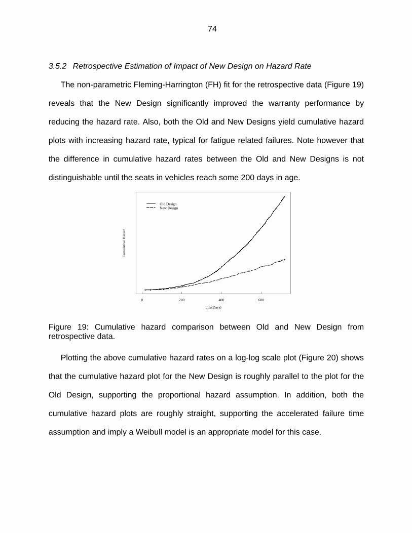
74

3.5.2 Retrospective Estimation of Impact of New Design on Hazard Rate

The non-parametric Fleming-Harrington (FH) fit for the retrospective data (Figure 19)

reveals that the New Design significantly improved the warranty performance by

reducing the hazard rate. Also, both the Old and New Designs yield cumulative hazard

plots with increasing hazard rate, typical for fatigue related failures. Note however that

the difference in cumulative hazard rates between the Old and New Designs is not

distinguishable until the seats in vehicles reach some 200 days in age.

Figure 19: Cumulative hazard comparison between Old and New Design from retrospective data.

Plotting the above cumulative hazard rates on a log-log scale plot (Figure 20) shows

that the cumulative hazard plot for the New Design is roughly parallel to the plot for the

Old Design, supporting the proportional hazard assumption. In addition, both the

cumulative hazard plots are roughly straight, supporting the accelerated failure time

assumption and imply a Weibull model is an appropriate model for this case.

Life(Days)

Cum

ulat

ive

Haz

ard

0 200 400 600

Old DesignNew Design

75

Figure 20: Cumulative hazard log-log scale plot comparing Old and New Design from retrospective data.

To estimate the impact of New Design in terms of or , we fitted the

retrospective data with a semi-parametric Cox PH model as well as a parametric

Weibull PH model. The results (Figure 21) show that both the Cox and Weibull models

fit the retrospective data reasonably well.

Figure 21: Cumulative hazard comparison among FH, Cox PH and Weibull PH models.

The estimations for the impact of the New Design in terms of or are almost

identical between Cox and Weibull PH models to the third decimal place, yielding a

Life(Days)

Cum

ulat

ive

Haz

ard

50 60 70 80 100 200 300 400 500 600 800

Old DesignNew Design

Life(Days)

Cum

ulat

ive

Haz

ard

0 200 400 600

FH-Old DesignCox-Old DesignFH-New DesignCox-New Design

Life(Days)

Cum

ulat

ive

Haz

ard

200 400 600

FH-Old DesignWeibull-Old DesignFH-New DesignWeibull-New Design

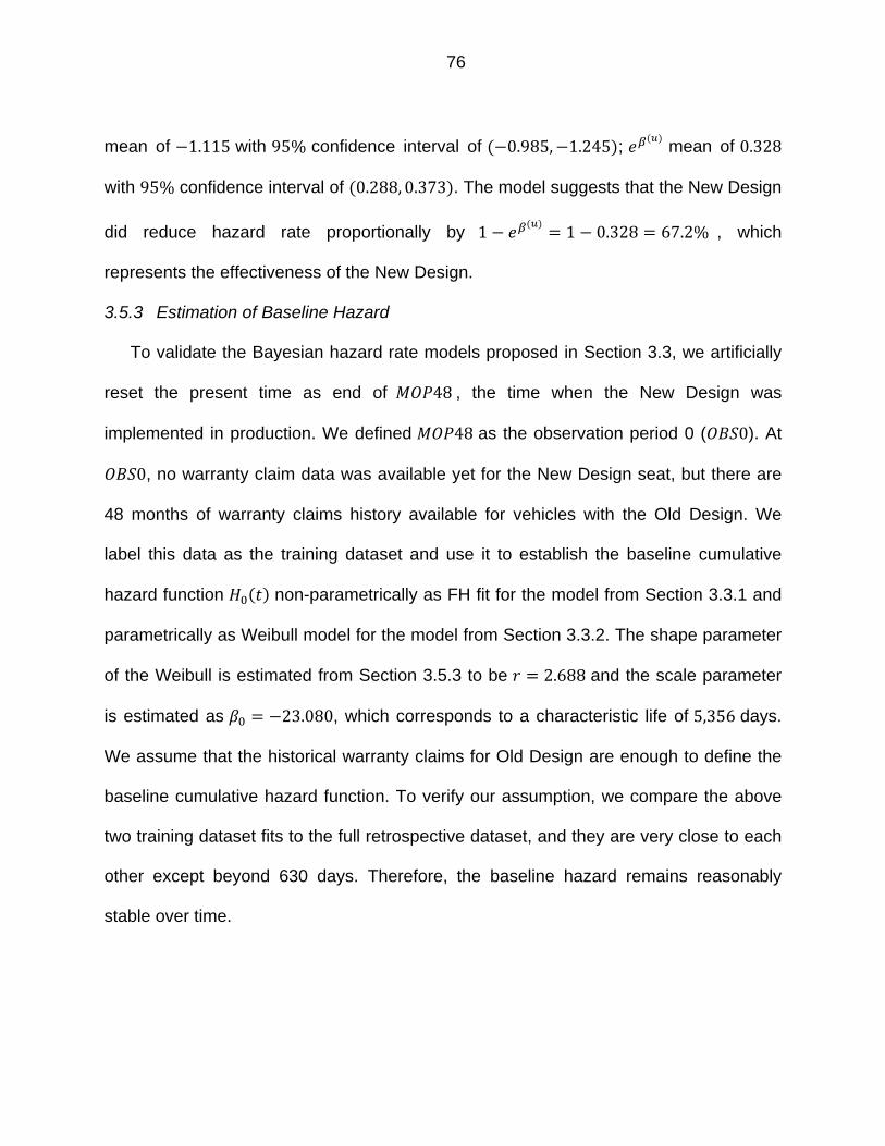
76

mean of 1.115 with 95% confidence interval of 0.985, 1.245 ; mean of 0.328

with 95% confidence interval of 0.288, 0.373 . The model suggests that the New Design

did reduce hazard rate proportionally by 1 1 0.328 67.2% , which

represents the effectiveness of the New Design.

3.5.3 Estimation of Baseline Hazard

To validate the Bayesian hazard rate models proposed in Section 3.3, we artificially

reset the present time as end of 48 , the time when the New Design was

implemented in production. We defined 48 as the observation period 0 ( 0). At

0, no warranty claim data was available yet for the New Design seat, but there are

48 months of warranty claims history available for vehicles with the Old Design. We

label this data as the training dataset and use it to establish the baseline cumulative

hazard function non-parametrically as FH fit for the model from Section 3.3.1 and

parametrically as Weibull model for the model from Section 3.3.2. The shape parameter

of the Weibull is estimated from Section 3.5.3 to be 2.688 and the scale parameter

is estimated as 23.080, which corresponds to a characteristic life of 5,356 days.

We assume that the historical warranty claims for Old Design are enough to define the

baseline cumulative hazard function. To verify our assumption, we compare the above

two training dataset fits to the full retrospective dataset, and they are very close to each

other except beyond 630 days. Therefore, the baseline hazard remains reasonably

stable over time.

77

Figure 22: Cumulative hazard comparison between FH, Weibull fits for training dataset and FH fit for full retrospective dataset.

3.5.4 Eliciting Prior Distribution of For the New Design

To obtain the prior distribution of New Design , we start with the objective testing

data. Before the New Design was released to production, three prototype from the New

Design as well as three Old Design production parts were each tested in the lab under

the same accelerated test cycle plan per design specification from the OEM. The test

results showed that all three Old Design samples failed and only one New Design

sample failed with the other two samples not failing at the end of the testing cycle

(censored). Given the limited testing data, we assume that the lab test follows the

typical Weibull AFT model with the same shape parameter as originally estimated in

Section 3.5.3 to be 2.688.

Life(Days)

Cum

ulat

ive

Haz

ard

0 100 200 300 400 500 600 700

TrainSet-FHTrainSet-WeibullFullSet-FH

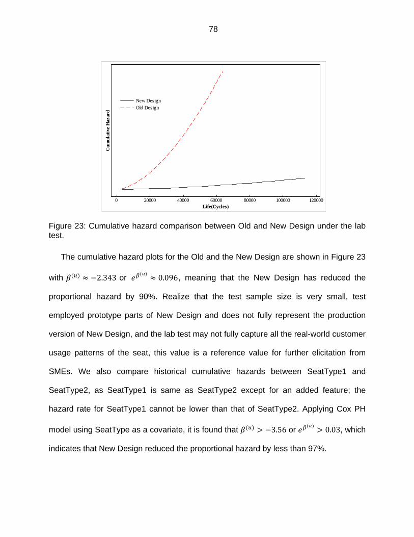
78

Figure 23: Cumulative hazard comparison between Old and New Design under the lab test.

The cumulative hazard plots for the Old and the New Design are shown in Figure 23

with 2.343 or 0.096, meaning that the New Design has reduced the

proportional hazard by 90%. Realize that the test sample size is very small, test

employed prototype parts of New Design and does not fully represent the production

version of New Design, and the lab test may not fully capture all the real-world customer

usage patterns of the seat, this value is a reference value for further elicitation from

SMEs. We also compare historical cumulative hazards between SeatType1 and

SeatType2, as SeatType1 is same as SeatType2 except for an added feature; the

hazard rate for SeatType1 cannot be lower than that of SeatType2. Applying Cox PH

model using SeatType as a covariate, it is found that 3.56 or 0.03, which

indicates that New Design reduced the proportional hazard by less than 97%.

120000100000800006000040000200000Life(Cycles)

Cum

ulat

ive

Haz

ard

New Design

Old Design

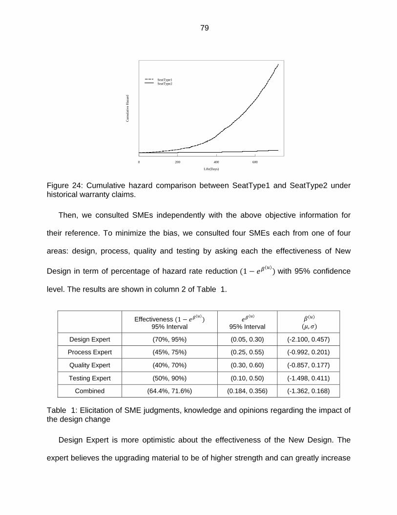
79

Figure 24: Cumulative hazard comparison between SeatType1 and SeatType2 under historical warranty claims.

Then, we consulted SMEs independently with the above objective information for

their reference. To minimize the bias, we consulted four SMEs each from one of four

areas: design, process, quality and testing by asking each the effectiveness of New

Design in term of percentage of hazard rate reduction 1 with 95% confidence

level. The results are shown in column 2 of Table 1.

Effectiveness 1 95% Interval

95% Interval

,

Design Expert (70%, 95%) (0.05, 0.30) (-2.100, 0.457)

Process Expert (45%, 75%) (0.25, 0.55) (-0.992, 0.201)

Quality Expert (40%, 70%) (0.30, 0.60) (-0.857, 0.177)

Testing Expert (50%, 90%) (0.10, 0.50) (-1.498, 0.411)

Combined (64.4%, 71.6%) (0.184, 0.356) (-1.362, 0.168)

Table 1: Elicitation of SME judgments, knowledge and opinions regarding the impact ofthe design change

Design Expert is more optimistic about the effectiveness of the New Design. The

expert believes the upgrading material to be of higher strength and can greatly increase

Life(Days)

Cum

ulat

ive

Haz

ard

0 200 400 600

SeatType1SeatType2

80

the seat structure resistance to fatigue; while Process and Quality Experts are more

pessimistic as they are more concerned about the increased production variation due to

new manufacturing processes induced by the material upgrading. Process and Quality

Experts also observed that certain new processes can degrade the material strength

and increase reject rate in the plant. All these are not reflected in prototype samples in

the lab test. Testing Expert is more concerned about the small sample size.

To combine the SME judgments, knowledge and opinions, we first assume that

is Gaussian distributed, therefore, is a log-normal distribution. Based on

the 95% interval of in column 3 of Table 1, we can derive the parameters of

, i.e., the mean and standard deviation . Then, we apply the simplest equal

weighted average combination method shown in Eq.(52) to derive the parameters for

the prior:

14

14

, ~ 1.362, 0.168 (52)

It follows that is log-normal with the same parameters, in which case, the

combined 95% confidence interval for can be derived as (0.184, 0.356).

To obtain the conjugate closed-form posterior, we need to evaluate in the

gamma distribution form. This can be done by fitting gamma to 95% confidence interval

(0.184, 0.356), which yields a shape parameter 35.764 and scale parameter

135.960.

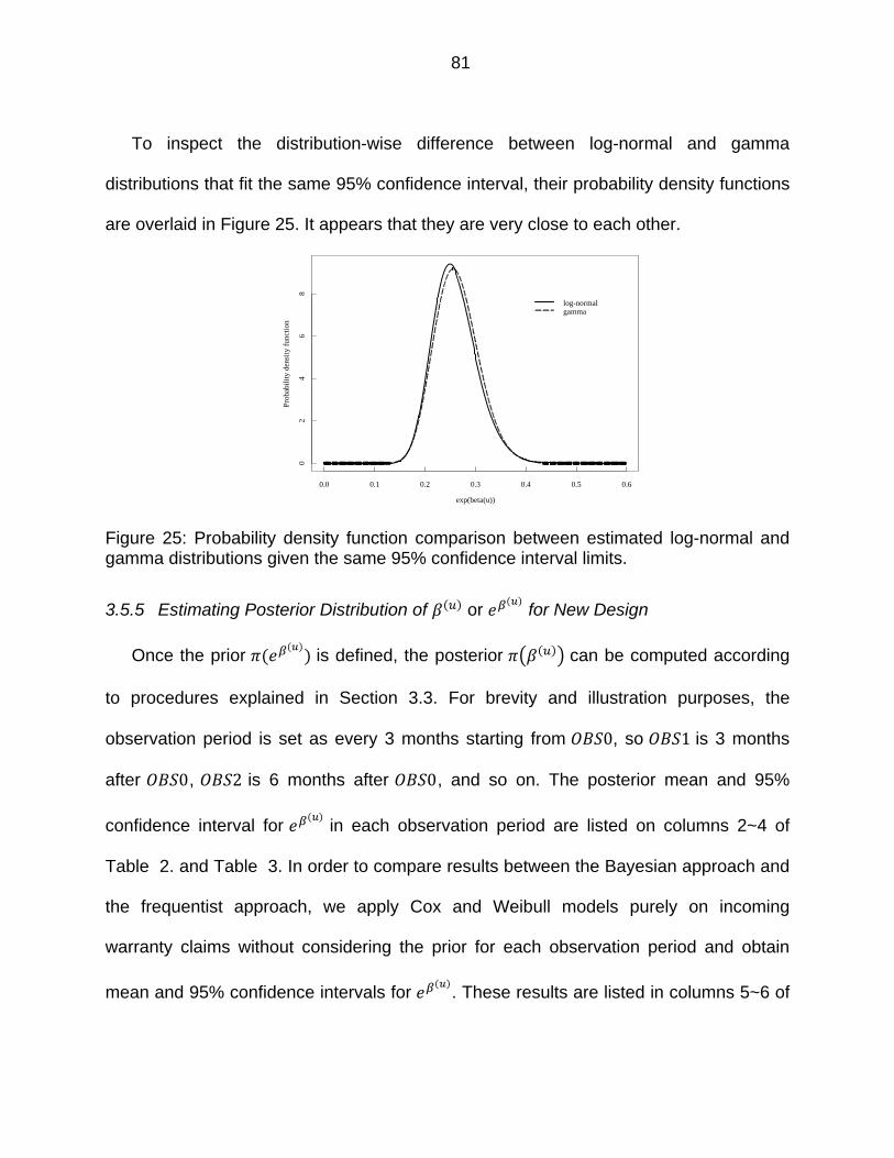
81

To inspect the distribution-wise difference between log-normal and gamma

distributions that fit the same 95% confidence interval, their probability density functions

are overlaid in Figure 25. It appears that they are very close to each other.

Figure 25: Probability density function comparison between estimated log-normal and gamma distributions given the same 95% confidence interval limits.

3.5.5 Estimating Posterior Distribution of or for New Design

Once the prior is defined, the posterior can be computed according

to procedures explained in Section 3.3. For brevity and illustration purposes, the

observation period is set as every 3 months starting from 0, so 1 is 3 months

after 0, 2 is 6 months after 0, and so on. The posterior mean and 95%

confidence interval for in each observation period are listed on columns 2~4 of

Table 2. and Table 3. In order to compare results between the Bayesian approach and

the frequentist approach, we apply Cox and Weibull models purely on incoming

warranty claims without considering the prior for each observation period and obtain

mean and 95% confidence intervals for . These results are listed in columns 5~6 of

exp(beta(u))

Prob

abil

ity

dens

ity

func

tion

0.0 0.1 0.2 0.3 0.4 0.5 0.6

02

46

8log-normalgamma

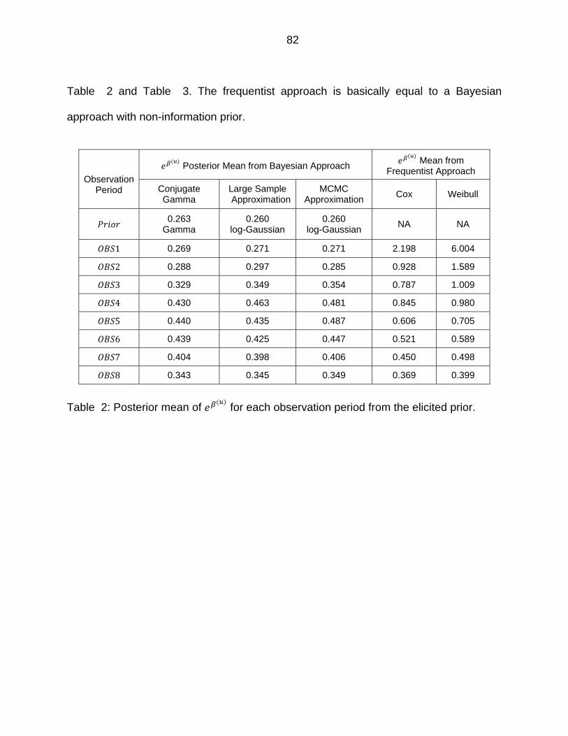
82

Table 2 and Table 3. The frequentist approach is basically equal to a Bayesian

approach with non-information prior.

Observation

Period

Posterior Mean from Bayesian Approach Mean from

Frequentist Approach

Conjugate Gamma

Large Sample Approximation

MCMC Approximation

Cox Weibull

0.263

Gamma 0.260

log-Gaussian 0.260

log-Gaussian NA NA

1 0.269 0.271 0.271 2.198 6.004

2 0.288 0.297 0.285 0.928 1.589

3 0.329 0.349 0.354 0.787 1.009

4 0.430 0.463 0.481 0.845 0.980

5 0.440 0.435 0.487 0.606 0.705

6 0.439 0.425 0.447 0.521 0.589

7 0.404 0.398 0.406 0.450 0.498

8 0.343 0.345 0.349 0.369 0.399

Table 2: Posterior mean of for each observation period from the elicited prior.

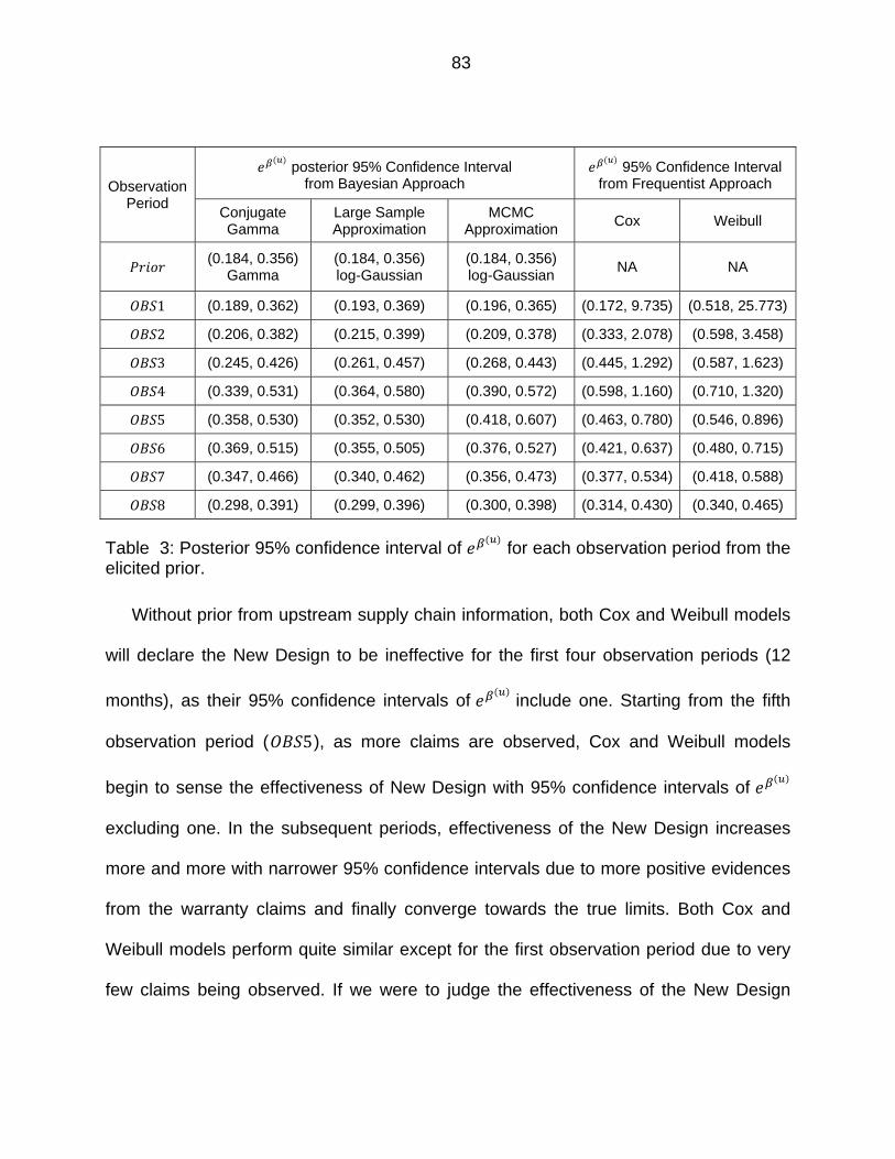
83

Observation Period

posterior 95% Confidence Interval from Bayesian Approach

95% Confidence Interval from Frequentist Approach

Conjugate Gamma


MCMC Approximation

Cox Weibull

(0.184, 0.356)

Gamma (0.184, 0.356) log-Gaussian

(0.184, 0.356) log-Gaussian

NA NA

1 (0.189, 0.362) (0.193, 0.369) (0.196, 0.365) (0.172, 9.735) (0.518, 25.773)

2 (0.206, 0.382) (0.215, 0.399) (0.209, 0.378) (0.333, 2.078) (0.598, 3.458)

3 (0.245, 0.426) (0.261, 0.457) (0.268, 0.443) (0.445, 1.292) (0.587, 1.623)

4 (0.339, 0.531) (0.364, 0.580) (0.390, 0.572) (0.598, 1.160) (0.710, 1.320)

5 (0.358, 0.530) (0.352, 0.530) (0.418, 0.607) (0.463, 0.780) (0.546, 0.896)

6 (0.369, 0.515) (0.355, 0.505) (0.376, 0.527) (0.421, 0.637) (0.480, 0.715)

7 (0.347, 0.466) (0.340, 0.462) (0.356, 0.473) (0.377, 0.534) (0.418, 0.588)

8 (0.298, 0.391) (0.299, 0.396) (0.300, 0.398) (0.314, 0.430) (0.340, 0.465)

Table 3: Posterior 95% confidence interval of for each observation period from the elicited prior.

Without prior from upstream supply chain information, both Cox and Weibull models

will declare the New Design to be ineffective for the first four observation periods (12

months), as their 95% confidence intervals of include one. Starting from the fifth

observation period ( 5), as more claims are observed, Cox and Weibull models

begin to sense the effectiveness of New Design with 95% confidence intervals of

excluding one. In the subsequent periods, effectiveness of the New Design increases

more and more with narrower 95% confidence intervals due to more positive evidences

from the warranty claims and finally converge towards the true limits. Both Cox and

Weibull models perform quite similar except for the first observation period due to very

few claims being observed. If we were to judge the effectiveness of the New Design

84

solely based on the warranty claims for the first four observation periods, we would

have generated a false alarm.

On the other hand, by extending hazard rate model to include prior from upstream

supply chain information, the effectiveness of the New Design is statistically significant

for all observation periods as none of 95% confidence interval of include one. The

effectiveness of the New Design decreases somewhat at the beginning due to limited

number of warranty claims to concur with the prior, but starting from the fifth observation

period, the effectiveness of the New Design becomes more apparent due to more

positive evidence from the warranty claims and finally converges towards the true

effectiveness. Our model effectively avoids false alarm on the effectiveness of New

Design in reducing warranty hazard rate.

As our hazard rate model from the Bayesian approach involves approximating using

the asymptotical normal distribution on large sample size in Section 3.3.1 and sampling

in Section 3.3.2, to evaluate their performance, their posterior means and the 95%

confidence interval of are compared with the "exact" posteriors from the conjugate

gamma prior; the results are reasonably close. For large sample size Bayesian

approach, the posterior means of are very close to the “exact” means with a

maximum 8% difference; the posterior 95% confidence intervals of are a little wider

(2~13%) than the “exact” ones. This is partially due to approximation and partially due to

different prior distributions.

The estimation of prior plays a key role in our hazard rate model from a Bayesian

approach. A better prior with mean closer to true mean and with a tighter confidence

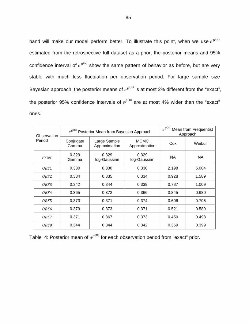
85

band will make our model perform better. To illustrate this point, when we use

estimated from the retrospective full dataset as a prior, the posterior means and 95%

confidence interval of show the same pattern of behavior as before, but are very

stable with much less fluctuation per observation period. For large sample size

Bayesian approach, the posterior means of is at most 2% different from the “exact”,

the posterior 95% confidence intervals of are at most 4% wider than the “exact”

ones.

Observation Period

Posterior Mean from Bayesian Approach Mean from Frequentist

Approach

Conjugate Gamma


MCMC Approximation

Cox Weibull

0.329

Gamma 0.329

log-Gaussian 0.329

log-Gaussian NA NA

1 0.330 0.330 0.330 2.198 6.004

2 0.334 0.335 0.334 0.928 1.589

3 0.342 0.344 0.339 0.787 1.009

4 0.365 0.372 0.366 0.845 0.980

5 0.373 0.371 0.374 0.606 0.705

6 0.379 0.373 0.371 0.521 0.589

7 0.371 0.367 0.373 0.450 0.498

8 0.344 0.344 0.342 0.369 0.399

Table 4: Posterior mean of for each observation period from "exact" prior.

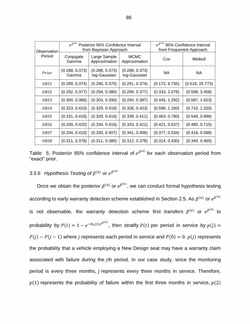
86

Observation Period

Posterior 95% Confidence Interval from Bayesian Approach

95% Confidence Interval from Frequentist Approach

Conjugate Gamma


MCMC Approximation

Cox Weibull

(0.288, 0.373)

Gamma (0.288, 0.373)log-Gaussian

(0.288, 0.373)log-Gaussian

NA NA

1 (0.289, 0.374) (0.290, 0.375) (0.291, 0.374) (0.172, 9.735) (0.518, 25.773)

2 (0.292, 0.377) (0.294, 0.380) (0.299, 0.377) (0.333, 2.078) (0.598, 3.458)

3 (0.300, 0.386) (0.303, 0.390) (0.294, 0.387) (0.445, 1.292) (0.587, 1.623)

4 (0.323, 0.410) (0.329, 0.419) (0.328, 0.423) (0.598, 1.160) (0.710, 1.320)

5 (0.331, 0.416) (0.329, 0.416) (0.339, 0.411) (0.463, 0.780) (0.546, 0.896)

6 (0.339, 0.420) (0.334, 0.416) (0.333, 0.421) (0.421, 0.637) (0.480, 0.715)

7 (0.334, 0.410) (0.330, 0.407) (0.341, 0.406) (0.377, 0.534) (0.418, 0.588)

8 (0.311, 0.378) (0.311, 0.380) (0.312, 0.378) (0.314, 0.430) (0.340, 0.465)

Table 5: Posterior 95% confidence interval of for each observation period from "exact" prior.

3.5.6 Hypothesis Testing of or

Once we obtain the posterior or e , we can conduct formal hypothesis testing

according to early warranty detection scheme established in Section 2.5. As or e

is not observable, the warranty detection scheme first transfers or e to

probability by 1 , then stratify per period in service by

1 where represents each period in service and 0 0. represents

the probability that a vehicle employing a New Design seat may have a warranty claim

associated with failure during the th period. In our case study, since the monitoring

period is every three months, represents every three months in service. Therefore,

1 represents the probability of failure within the first three months in service, 2

87

represents the probability between three and six months in service, and so on. We set

our total monitoring periods as eight ( 8), covering a total of twenty-four months in

service.

As illustrated in Chapter 2, the warranty detection scheme determines upper and

lower warranty claim limits for each period in service through the Binomial distribution.

The observed warranty claims will be compared with the upper and lower limits for

hypothesis testing.

As each stratified is assumed to be independent, the warranty detection

scheme can conduct multiple hypothesis tests independently, for each period in service.

We set overall false alarm probability at 0.1% consistent with (Wu and Meeker,

2002), then the overall false alarm probability is allocated to each period in service

based on Eq.(13). Since in our case study detection of New Design effectiveness is

critical, and we believe that the effectiveness will demonstrate itself more in later

periods in service due to increasing hazard rate exhibited in Figure 19, larger values will

be assigned to from later periods in service.

The hypothesis test results are summarized in Figure 26 to Figure 33. The actual

claim rates are masked to protect proprietary and confidential information, however all

figures are kept at the same scale for relative comparison. The figures show that the

effectiveness of the New Design is predicted well up to twenty-four months in service.

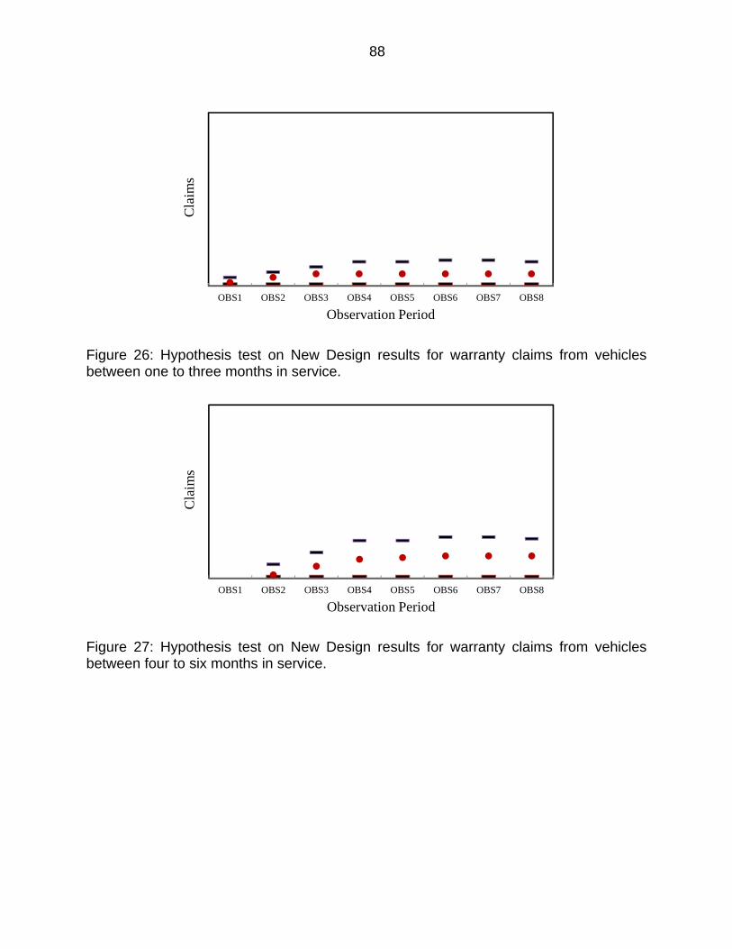
88

Figure 26: Hypothesis test on New Design results for warranty claims from vehicles between one to three months in service.

Figure 27: Hypothesis test on New Design results for warranty claims from vehicles between four to six months in service.

OBS1 OBS2 OBS3 OBS4 OBS5 OBS6 OBS7 OBS8

Cla

ims

Observation Period


Cla

ims

Observation Period

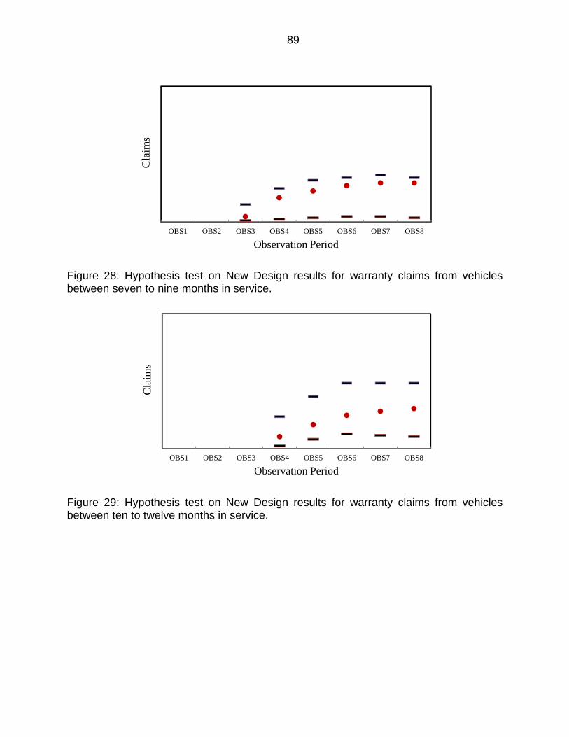
89

Figure 28: Hypothesis test on New Design results for warranty claims from vehicles between seven to nine months in service.

Figure 29: Hypothesis test on New Design results for warranty claims from vehicles between ten to twelve months in service.


Cla

ims

Observation Period


Cla

ims

Observation Period

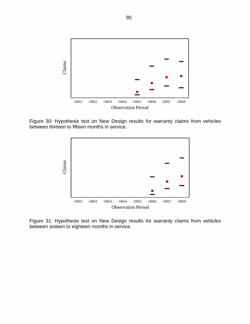
90

Figure 30: Hypothesis test on New Design results for warranty claims from vehicles between thirteen to fifteen months in service.

Figure 31: Hypothesis test on New Design results for warranty claims from vehicles between sixteen to eighteen months in service.


Cla

ims

Observation Period


Cla

ims

Observation Period

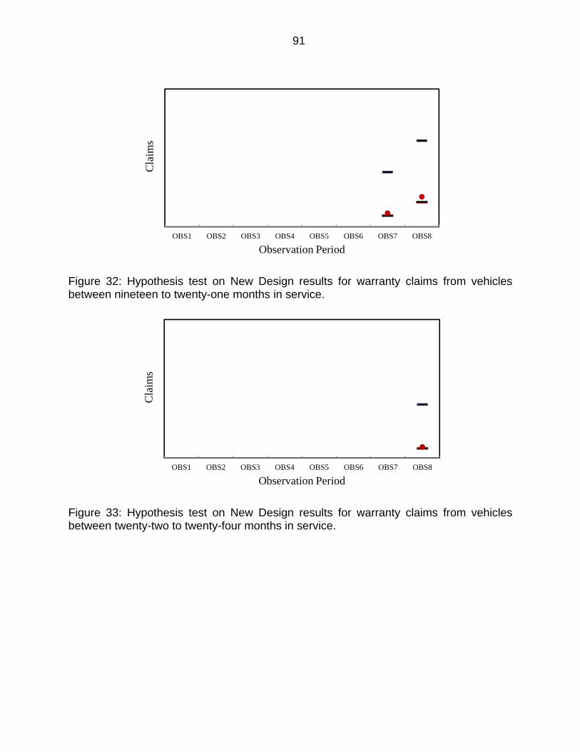
91

Figure 32: Hypothesis test on New Design results for warranty claims from vehicles between nineteen to twenty-one months in service.

Figure 33: Hypothesis test on New Design results for warranty claims from vehicles between twenty-two to twenty-four months in service.


Cla

ims

Observation Period


Cla

ims

Observation Period

92

3.5.7 Performance Review: Large Sample Size vs. MCMC Bayesian Analysis

Even though the output results from the two Bayesian analysis are very close

(Table 2 to Table 5), large sample size method definitely outperforms MCMC method

on computation efficiency. Except PH model estimation from SPlus, large sample size

Bayesian analysis does not require specialized software to obtain the posterior, so the

posterior is obtained instantaneously, but MCMC Bayesian analysis requires both SPlus

for PH model estimation and a specialized software (e.g. WinBUGS) for posterior

estimation. For the large dataset in our case study, the run-times for convergent

posteriors can be very long: it easily requires more than 10,000 iterations for 4 CPU

hours under AMD quad-core 2.8GHz processor with 16G ram. Also the convergence

cannot be guaranteed and sensitive to the choice of initial value.

3.6 Conclusion

In this chapter, we have extended our earlier hazard rate models by incorporating

upstream supply chain information as priors through the Bayesian approach. This

allows us to evaluate the impacts from brand new design/process changes on warranty

performance even though there is no associated historical warranty claims available. By

properly eliciting priors via objective data and SME knowledge, judgments and opinions

available from suppliers, such impacts can be detected earlier with more power.

Through proper priors, our model can avoid false alarms effectively during early

warranty detection.

Also, by utilizing historical warranty claims associated with upstream supply chain

information, our model relieves us from the heavy computational burden by avoiding

93

estimating the posterior baseline hazard function. This will make our model more

practical and computationally efficient. The case study shows that our models perform

rather well.

94

CHAPTER 4 SUMMARY AND CONCLUSIONS

4.1 Summary and Research Contribution

The automotive industry spends $10-$13 billion per year on warranty claim (Arnum,

2011b) which consumes roughly 1- 5.2% of OEMs’ product revenue and roughly 0.5-1%

of suppliers’ product revenue (Arnum, 2011a). Early detection of reliability problem can

help OEMs and suppliers to take corrective actions as quick as possible to minimize

warranty cost and reputation damage due to poor reliability.

Reducing warranty costs and improving product reliability is the joint objective and

responsibility of OEMs and suppliers. As we know, a vehicle consists of many

modularized subsystems and thousands of components which are supplied through

suppliers at different tier levels. Before a vehicle is produced, these subsystems,

components have to go through design, testing and manufacturing process on suppliers’

sites. Therefore reliability problems don’t just start from vehicles reaching customer’s

hands, but can start far early at suppliers’ sites and are heavily influenced by operations

at all tiers of suppliers as shown in Figure 1.There is a wealth of upstream supply chain

information that exists long before vehicles are built but not being exploited. If this prior

upstream information can be utilized in a statistical framework to correlate to warranty

claims, the warranty issues and the effectiveness of corrective actions to address these

issues may be predicted and detected earlier with more power

This research provides effective methods for suppliers to link their upstream supply

chain information to warranty claims. The proposed models adopts hazard rate concept

which is a well understood concept in the reliability engineering community, organizes

95

the abundant but diversified upstream supply chain information into explanatory

covariates and associates them with each vehicle and assuming their impact to hazard

rate as constant multiples of each other.

When the covariates have direct historical warranty claims, the proposed model

uses frequentist approach to establish their impacts as regression coefficients of the

covariates directly from historical warranty claims. When the current covariates' values

are available and known to suppliers, and before the vehicles associated with these

covariates are serviced in the field, the established regression coefficients can be used

to predict warranty claims rates from the field. Such predictions can be tested

sequentially through hypothesis tests during each monitoring period in term of number

of claims through the Binomial model.

When the covariates do not have direct historical warranty claims, the proposed

model recommends a Bayesian approach to establish their impacts as regression

coefficients of the covariates through priors elicited from SMEs, judgments and opinions.

The priors are updated sequentially as posteriors every monitoring period as warranty

claims become available. The posteriors can be used to predict warranty claim rates

from the field. Again, these claim rates can be tested sequentially through hypothesis

tests during every monitoring period through the Binomial model. To avoid heavy

computation burden to estimate the posterior, the proposed model further utilizes any

existing upstream supply chain information to establish the baseline hazard function, so

that it is known and fixed during the Bayesian modeling.

96

The proposed model is practical to suppliers as the concept is more engineering

oriented, moreover it is easy to apply as most statistical software have standard

modules to implement this model without writing advanced codes.

The proposed model can help to address the following sorts of industry based

problems especially from a supplier’s perspective:

If we know status quo in suppliers' product, can we know the future warranty

performance?

How to verify what we claim to know?

How to detect and detect earlier if what we claim to know is wrong?

4.2 Limitations and Recommendations for Future Research

As the proposed models are from a supplier’s point of view, focuses on linking

warranty claim rates to design and inherent reliability, to which the upstream supply

chain information are available and can be extracted and on which a supplier has a

control, it assumes sale reliability due to transportation and storage, field reliability due

to operating environment, usage mode/intensity and customer behavior are

homogeneous over production periods. This reduces the need for collecting information

regarding these factors. However these factors can be important factors impacting

warranty claims; for example, the percentage of warranty claims due to user behavior

can be as large as 10%+ (Wu, 2011). If the levels of heterogeneity for these factors are

high over production periods, the models can be extended to account for those

heterogeneities. If these factors can be transformed to explanatory covariates, for

example, vehicles can be segmented as qualitative covariates by sold geographic

97

region such as Northeast, Midwest, South and West in US to account for heterogeneity

of operating environment; by sold country to account for heterogeneity of customer

behavior; by sold type such as retail and fleet to account for heterogeneity of usage

mode/intensity, by transportation route to account for heterogeneity of

transportation/storage, they can be easily incorporated into the proposed models as

additional covariates which can further improve the detection power of the proposed

models. Frailty models are also candidates to model hazard rates in the presence of

over-dispersion or group-specific random effects (Glidden and Vittinghoff, 2004). The

latter are distinguished from the former by the term “shared” frailty models.

Unfortunately, such data is not currently available to suppliers from OEM warranty

databases.

The proposed model also assumes proportional hazards with respect to all

covariates, as it provides a simple and easy way to estimate the effects of covariates.

When the proportionality assumption of the hazard rate model does not hold, the time

periods can be divided into several sub-time periods such that proportionality holds

within each sub-time period, then, one can fit separate hazard rate models for each sub-

time period.

98

REFERENCES

AIAG, 2008. Consumer-centric Warranty Management: A Guideline For Industry Best

Practices (CQI-14), 1 ed. Automotive Industry Action Group (AIAG), Southfield,

Michigan, USA.

Akaike, H., 1974. A new look at the statistical model identification. IEEE Transaction on

Automatic Control 19, 716-723.

Arnum, E., 2011a. Automotive Warranty Report, Warranty Week.

Arnum, E., 2011b. Eighth Annual Warranty Report,Totals & Averages, Warranty Week.

Attardi, L., Guida, M., Pulcini, G., 2005. A mixed-Weibull regression model for the

analysis of automotive warranty data. Reliability Engineering & System Safety 87,

265-273.

Blischke, W.R., Murthy, D.N.P., 1996. Product warranty handbook. M. Dekker, New

York.

Booker, J., Bement, T., Meyer, M., Kerscher, W., 2003. PREDICT: a new approach to

product development and lifetime assessment using information integration

technology, in: Khattree, C., Rao, R. (Eds.), Handbook of statistics: statistics in

industry.

Booker, J., Singpurwalla, N.D., 2003. Using Probability and Fuzzy Set Theory for

Reliability Assessment, Proc. 21st Int. Modal Analysis Conference (IMAC-XXI),,

Kissimmee, FL, p. 259.

99

Booker, J.M., McNamara, L.A., 2004. Solving black box computation problems using

expert knowledge theory and methods. Reliability Engineering & System Safety 85,

331-340.

Canavos, G.C., Tsokos, C.P., 1973. Bayesian Estimation of Life Parameters in the

Weibull Distribution. Operations Research 21, 755-763.

Carty, S.S., 2010. Toyota's $16.4 million fine a small slice of total recall costs, USA

Today.

Clemen, R., Jones, S., Winkler, R., 1996. Aggregating forecasts: An empirical

evaluation of some Bayesian methods. In D. Berry, K. Chaloner, & J. Geweke (Eds.),

Bayesian Statistics and Econometrics: Essays in Honor of Arnold Zellner, 3–13.

Clemen, R.T., Winkler, R.L., 1999. Combining Probability Distributions From Experts in

Risk Analysis. Risk Analysis 19, 187-203.

Cook, J.D., 2010. Determining distribution parameters from quantiles, UT MD Anderson

Cancer Center Department of Biostatistics Working Paper Series, p. Working Paper

55.

Cooke, N.J., 1994. Varieties of knowledge elicitation techniques. International Journal of

Human-Computer Studies 41, 801-849.

Cox, D., 1972. Regression Models and Life-Tables. Journal of the Royal Statistical

Society, Series B (Methodological) 34, 33.

Cox, D.R., 1975. Partial Likelihood. Biometrika 62, 269-276.

Cox, D.R., Hinkley, D.V., 1974. Theoretical Statistics. Chapman and Hall, London.

Doksum, K., 1974. Tailfree and Neutral Random Probabilities and Their Posterior

Distributions. The Annals of Probability 2, 183-201.

100

Faraggi, D., Simon, R., 1997. Large sample Bayesian inference on the parameters of

the proportional hazard models. Statistics in Medicine 16, 2573-2585.

Ferguson, T.S., 1973. A Bayesian Analysis of Some Nonparametric Problems. The

Annals of Statistics 1, 209-230.

Fredette, M., Lawless, J.F., 2007. Finite-horizon prediction of recurrent events, with

application to forecasts of warranty claims. Technometrics 49, 66-80.

Gelfand, A.E., Mallick, B.K., 1995. Bayesian Analysis of Proportional Hazards Models

Built from Monotone Functions. Biometrics 51, 843-852.

Gelfand, A.E., Smith, A.F.M., 1990. Sampling-Based Approaches to Calculating

Marginal Densities. Journal of the American Statistical Association 85, 398-409.

Glidden, D.V., Vittinghoff, E., 2004. Modelling clustered survival data from multicentre

clinical trials. Statistics in Medicine 23, 369-388.

Grabert, M., Prechtel, M., Hrycej, T., Gunther, W., 2004. An early warning system for

vehicle related quality data, Advances in Data Mining, pp. 88-95.

Hardin, J.W., Hilbe, J., M., 2007. Generalized Linear Models and Extensions, 2nd

Edition. StataCorp LP.

Helsen, K., Schmittlein, D.C., 1993. ANALYZING DURATION TIMES IN MARKETING -

EVIDENCE FOR THE EFFECTIVENESS OF HAZARD RATE MODELS. Marketing

Science 12, 395-414.

Hjort, N.L., 1990. Nonparametric Bayes Estimators Based on Beta Processes in Models

for Life History Data. The Annals of Statistics 18, 1259-1294.

Hosmer, D.W., Lemeshow, S., May, S., 2008. Applied Survival Analysis: Regression

Modeling of Time to Event Data. Wiley-Interscience.

101

Hu, X.J., Lawless, J.F., 1996. Estimation from truncated lifetime data with

supplementary information on covariates and censoring times. Biometrika 83, 747-

761.

Hu, X.J., Lawless, J.F., 1997. Pseudolikelihood estimation in a class of problems with

response-related missing covariates. Can. J. Stat.-Rev. Can. Stat. 25, 125-142.

Kalbfleisch, J.D., 1978. Non-Parametric Bayesian Analysis of Survival Time Data.

Journal of the Royal Statistical Society. Series B (Methodological) 40, 214-221.

Kalbfleisch, J.D., Lawless, J.F., 1991. REGRESSION-MODELS FOR RIGHT

TRUNCATED DATA WITH APPLICATIONS TO AIDS INCUBATION TIMES AND

REPORTING LAGS. Stat. Sin. 1, 19-32.

Kalbfleisch, J.D., Lawless, J.F., Robinson, J.A., 1991. METHODS FOR THE ANALYSIS

AND PREDICTION OF WARRANTY CLAIMS. Technometrics 33, 273-285.

Karim, R., Suzuki, K., 2005. Analysis of warranty claim data: a literature review. The

International Journal of Quality & Reliability Management 22.

Kim, S., Ibrahim, J., 2000. On Bayesian Inference for Proportional Hazards Models

Using Noninformative Priors. Lifetime Data Analysis 6, 331-341.

Kim, Y., Lee, J., 2003. Bayesian Analysis of Proportional Hazard Models. The Annals of

Statistics 31, 493-511.

King, G., 1988. Statistical Models for Political Science Event Counts: Bias in

Conventional Procedures and Evidence for the Exponential Poisson Regression

Model. American Journal of Political Science 32, pp. 838-863.

Klein, J.P., Moeschberger, M.L., 2003. Survival analysis : techniques for censored and

truncated data, 2nd ed. Springer, New York.

102

Kleyner, A., Sandborn, P., 2005. A warranty forecasting model based on piecewise

statistical distributions and stochastic simulation. Reliability Engineering & System

Safety 88, 207-214.

Krivtsov, V., Frankstein, M., 2004. Nonparametric estimation of marginal failure

distributions from dually censored automotive data, Annual Reliability and

Maintainability Symposium, 2004 Proceedings, pp. 86-89.

Lawless, J.F., 1994. ADJUSTMENTS FOR REPORTING DELAYS AND THE

PREDICTION OF OCCURRED BUT NOT REPORTED EVENTS. Can. J. Stat.-Rev.

Can. Stat. 22, 15-31.

Lawless, J.F., 1995. THE ANALYSIS OF RECURRENT EVENTS FOR MULTIPLE

SUBJECTS. Applied Statistics-Journal of the Royal Statistical Society Series C 44,

487-498.

Lawless, J.F., 1998. Statistical analysis of product warranty data. International

Statistical Review 66, 41-60.

Lawless, J.F., 2003. Statistical models and methods for lifetime data, 2nd ed. Wiley-

Interscience, Hoboken, N.J.

Lawless, J.F., Nadeau, C., 1995. SOME SIMPLE ROBUST METHODS FOR THE

ANALYSIS OF RECURRENT EVENTS. Technometrics 37, 158-168.

Lee, S., Seo, S., Yeom, S., Moon, K., Kang, M., Kim, B., 2007. A Study on

Warning/Detection Degree of Warranty Claims Data Using Neural Network Learning,

Advanced Language Processing and Web Information Technology, 2007. ALPIT

2007. Sixth International Conference on, pp. 492 - 497.

103

Li, Z.G., Zhou, S.Y., Choubey, S., Sievenpiper, C., 2007. Failure event prediction using

the Cox proportional hazard model driven by frequent failure signatures. IIE

Transactions 39, 303-315.

Lindley, D.V., Smith, A.F.M., 1972. Bayes Estimates for the Linear Model. Journal of the

Royal Statistical Society. Series B (Methodological) 34, 1-41.

Lindner, G., Klose, A., 1997. ML and Statistics for Trend Prognosis of complaints in the

Automobile Industry, Proceedings of the ICML-97 Workshop on Machine Learning

Applications in the Real World: Methodological Aspects and Implication.

Lindner, G., Studer, R., 1999. Forecasting the Fault Rate Behavior for Cars Workshop

proceedings from the ICML 1999, March 1999 ed.

Majeske, K.D., 2003. A mixture model for automobile warranty data. Reliability

Engineering & System Safety 81, 71-77.

Majeske, K.D., 2007. A non-homogeneous Poisson process predictive model for

automobile warranty claims. Reliability Engineering & System Safety 92, 243-251.

Majeske, K.D., LynchCaris, T., Herrin, G., 1997. Evaluating product and process design

changes with warranty data. International Journal of Production Economics 50, 79-

89.

Mohan, K., Cline, B., Akers, J., 2008. A practical method for failure analysis using

incomplete warranty data, Reliability and Maintainability Symposium, 2008. RAMS

2008. Annual, 28-31 Jan. 2008 ed, pp. 193 - 199

MSX, 2010. Integrated Warranty Solutions – White Paper.

Murthy, P., 2010. New research in reliability, warranty and maintenance, in: Stefanka

Chukova, J.H.a.T.D. (Ed.), 4th Asia-Pacific International Symposium on Advanced

104

Reliability and Maintenance Modeling (APARM 2010). McGraw-Hill International

Enterprises, Wellington, New Zealand, pp. 504-515.

OESA, 2005. The Suppliers Practical Guide to Warranty Reduction. Original Equipment

Suppliers Association (OESA), Troy, Michigan, USA.

Oh, Y.S., Bai, D.S., 2001. Field data analyses with additional after-warranty failure data.

Reliability Engineering & System Safety 72, 1-8.

Oleinick, P., 2004. Using reliability growth models to detect emerging warranty

problems. ASQ Conference on Lean Quality: The Coming Revolution in Reducing

Warranty Expense.

Rai, B., Singh, N., 2003. Hazard rate estimation from incomplete and unclean warranty

data. Reliability Engineering & System Safety 81, 79-92.

Rai, B., Singh, N., 2004. Modeling and analysis of automobile warranty data in presence

of bias due to customer-rush near warranty expiration limit. Reliability Engineering &

System Safety 86, 83-94.

Singpurwalla, N.D., 1988a. Foundational Issues in Reliability and Risk Analysis. SIAM

Review 30, 264-282.

Singpurwalla, N.D., 1988b. AN INTERACTIVE PC-BASED PROCEDURE FOR

RELIABILITY ASSESSMENT INCORPORATING EXPERT OPINION AND

SURVIVAL-DATA. Journal of the American Statistical Association 83, 43-51.

Singpurwalla, N.D., 2006. Reliability and risk : a Bayesian perspective. J. Wiley & Sons,

Chichester, West Sussex, England; New York.

Sinha, D., Dey, D.K., 1997. Semiparametric Bayesian Analysis of Survival Data. Journal

of the American Statistical Association 92, 1195-1212.

105

Smith, A.F.M., Gelfand, A.E., 1992. Bayesian Statistics without Tears: A Sampling-

Resampling Perspective. The American Statistician 46, 84-88.

Soyer, R., Tarimcilar, M.M., 2008. Modeling and Analysis of Call Center Arrival Data: A

Bayesian Approach. MANAGEMENT SCIENCE 54, 266-278.

Takahashi, Y., 2010. Toyota Registers Surprise Profit The Wall Stree Journal.

Toyota, 2010. Recall information.

Tsokos, C.P., Canavos, G.C., 1972. Bayesian Concepts for the Estimation of Reliability

in the Weibull Life-Testing Model. International Statistical Review / Revue

Internationale de Statistique 40, 153-160.

Wu, H.Q., Meeker, W.Q., 2002. Early detection of reliability problems using information

from warranty databases. Technometrics 44, 120-133.

Wu, S., 2011. Warranty claim analysis considering human factors. Reliability


Wu, S., Akbarov, A., 2011. Support vector regression for warranty claim forecasting.

European Journal of Operational Research 213, 196-204.

Yadav, O.P., Singh, N., Chinnam, R.B., Goel, P.S., 2003. A fuzzy logic based approach

to reliability improvement estimation during product development. Reliability


Yang, G.B., Zaghati, Z., 2002. Two-dimensional reliability modeling from warranty data,

Annual Reliability and Maintainability Symposium, 2002 Proceedings, pp. 272-278.

Zuashkiani, A., Banjevic, D., Jardine, A.K.S., 2006. Incorporating expert knowledge

when estimating parameters of the proportional hazards model, Proceedings of the

106

RAMS '06. Annual Reliability and Maintainability Symposium, 2006. IEEE Computer

Society, pp. 402-408.

107

ABSTRACT

HAZARD RATE MODELS FOR EARLY WARRANTY ISSUE DETECTION USING UPSTREAM SUPPLY CHAIN INFORMATION

by

CHONGWEN ZHOU

December 2011

Advisor: Dr. Ratna Babu Chinnam

Major: Industrial Engineering

Degree: Doctor of Philosophy

This research presents a statistical methodology to construct an early automotive

warranty issue detection model based on upstream supply chain information. This is

contrary to extant methods that are mostly reactive and only rely on data available from

the OEMs (original equipment manufacturers). For any upstream supply chain

information with direct history from warranty claims, the research proposes hazard rate

models to link upstream supply chain information as explanatory covariates for early

detection of warranty issues. For any upstream supply chain information without direct

warranty claims history, we introduce Bayesian hazard rate models to account for

uncertainties of the explanatory covariates. In doing so, it improves both the accuracy of

warranty issue detection as well as the lead time for detection. The proposed

methodology is illustrated and validated using real-world data from a leading global Tier-

one automotive supplier.

108

AUTOBIOGRAPHICAL STATEMENT

CHONGWEN ZHOU PROFESSIONAL EXPERIENCE: Skilled professional with proven management experience. More than 11 years experience in warranty, quality, reliability, 4 years experience in product design and 2 years teaching experience. Strong background in automotive industry. Proven track record of root cause and warranty analysis. 12/2007-present: Warranty and SR Manager - Faurecia Automotive Seating Inc.,

Troy, MI, USA. 05/2007-12/2007: Customer Quality Supervisor - Sanden International, Plymouth, MI,

USA. 03/2004 - 05/2007: Warranty Supervisor - Faurecia Automotive Seating Inc., Troy,

MI, USA. 05/2000 - 03/2004: Warranty/Reliability Engineer - Ford Motor Company, Dearborn,

MI, USA 03/1998 - 05/2000: Teaching Assistant - Wayne State University, Detroit, MI, USA 03/1997 - 03/1998: Product Engineer - Thomson Multimedia Asia Pte Ltd, Singapore 03/1996 - 03/1997: Product Engineer - Hewlett-Packard Singapore Pte Ltd,

Singapore 11/1994 - 03/1996: Product Engineer - Avimo Electro-Optics Pte Ltd, Singapore EDUCATION: Master of Mechanical Engineering, National University of Singapore, 1994 Master of Mechanics, Beijing University, 1992 Bachelor of Mechanics, Beijing University, 1989 CERTIFICATES: Certified Six Sigma Black Belt, American Society for Quality Certified Quality Engineer, American Society for Quality Certified Reliability Engineer, American Society for Quality Certified ISO/TS 16949:2002 Lead Supplier Auditor, RAB-QSA Recipient of Ford Extraordinary Effort/Performance Recognition Award PUBLICATIONS: Author or co-author of 4 journal papers covering topics in biomedical engineering, fluid mechanics, and product design/reliability.

Documents

Hazard rate models for early warranty issue detection