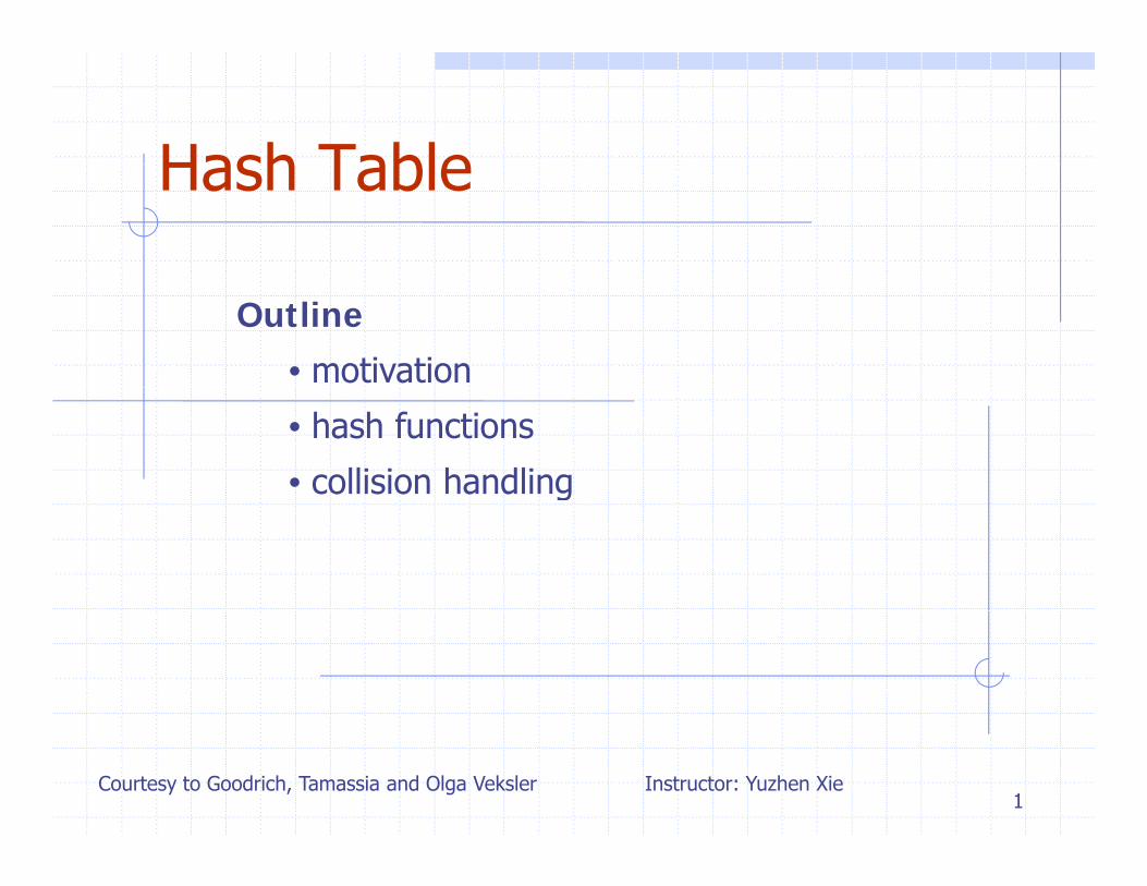
Hash TableHash Table

Outline• motivation

• hash functions

• collision handlingg

1Courtesy to Goodrich, Tamassia and Olga Veksler Instructor: Yuzhen Xie

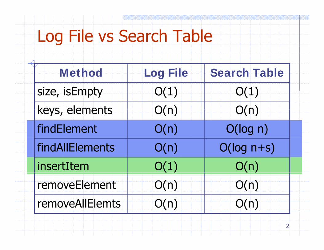
Log File vs Search Table

Method Log File Search Tableg

size, isEmpty O(1) O(1)

keys elements O(n) O(n)keys, elements O(n) O(n)

findElement O(n) O(log n)

findAllElements O(n) O(log n+s)

insertItem O(1) O(n)( ) ( )

removeElement O(n) O(n)

removeAllElemts O(n) O(n)

2

removeAllElemts O(n) O(n)

Hash Table MotivationHash Table Motivation

Efficient operations, insert, search, delete, to work with a dynamic set of data.

3

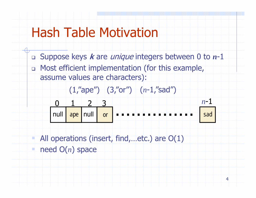
Hash Table MotivationHash Table Motivation

Suppose keys k are unique integers between 0 to n-1Most efficient implementation (for this example, assume values are characters):

( ” ”) ( ” ”) ( ” d”)(1,”ape”) (3,”or”) (n-1,”sad”)

0 1 2 3 n-1

ll llll ll ll

All ti (i t fi d t ) O(1)

……………null nullnull null nullsadape or

All operations (insert, find,…etc.) are O(1)need O(n) space

4

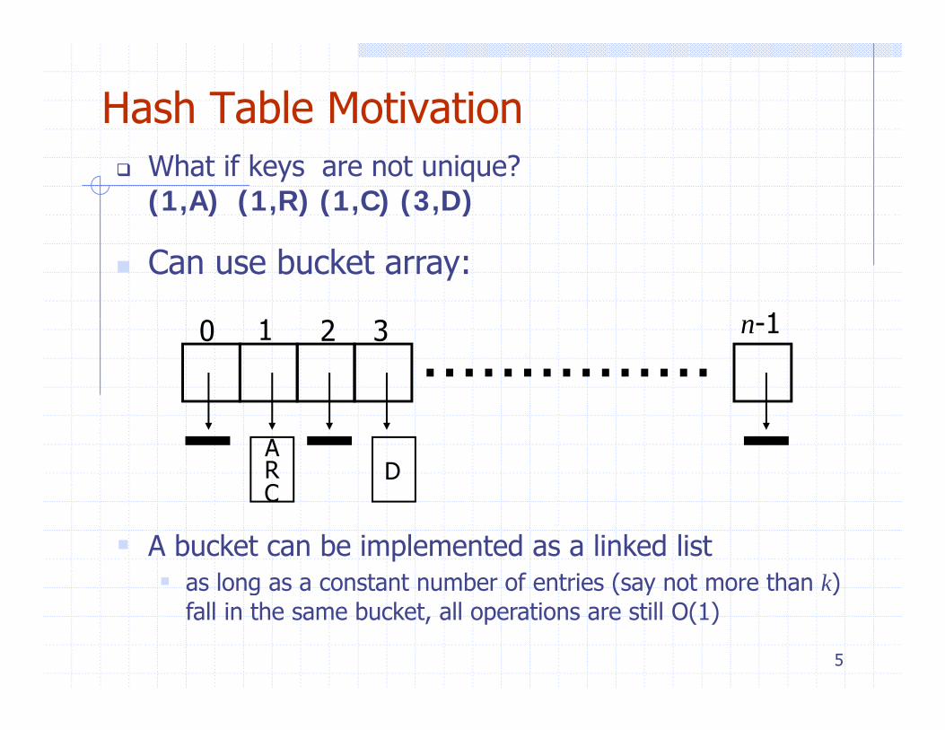
Hash Table MotivationWhat if keys are not unique? (1,A) (1,R) (1,C) (3,D)

1 1

Can use bucket array:

……………0 1 2 3 n-1

ARC

D

A bucket can be implemented as a linked listas long as a constant number of entries (say not more than k)

5

g ( y )fall in the same bucket, all operations are still O(1)

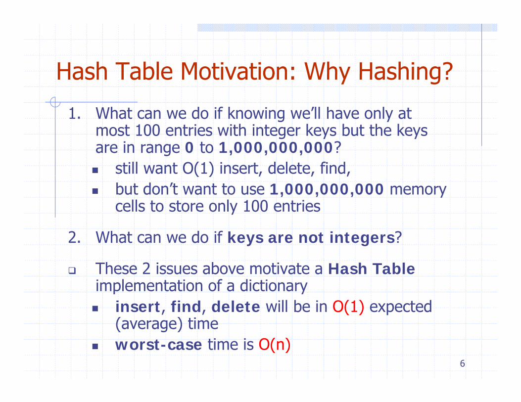
Hash Table Motivation: Why Hashing?Hash Table Motivation: Why Hashing?

1. What can we do if knowing we’ll have only at t 100 t i ith i t k b t th kmost 100 entries with integer keys but the keys

are in range 0 to 1,000,000,000?still want O(1) insert, delete, find, ( ) , , ,but don’t want to use 1,000,000,000 memory cells to store only 100 entries

2. What can we do if keys are not integers?

These 2 issues above motivate a Hash Table implementation of a dictionary

insert, find, delete will be in O(1) expected (average) time

6

(average) timeworst-case time is O(n)

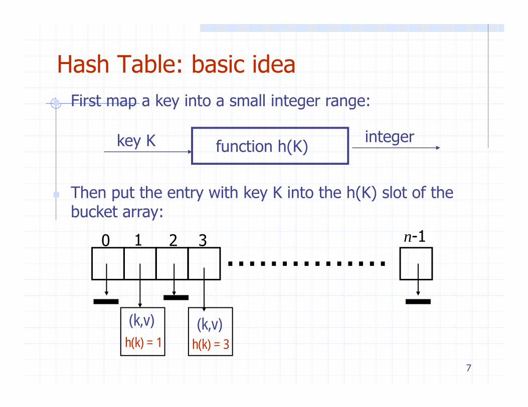
Hash Table: basic ideaFirst map a key into a small integer range:

function h(K)key K integer

Then put the entry with key K into the h(K) slot of the bucket array:

……………0 1 2 3 n-1

(k,v) (k,v)

7

h(k) = 1 h(k) = 3( )

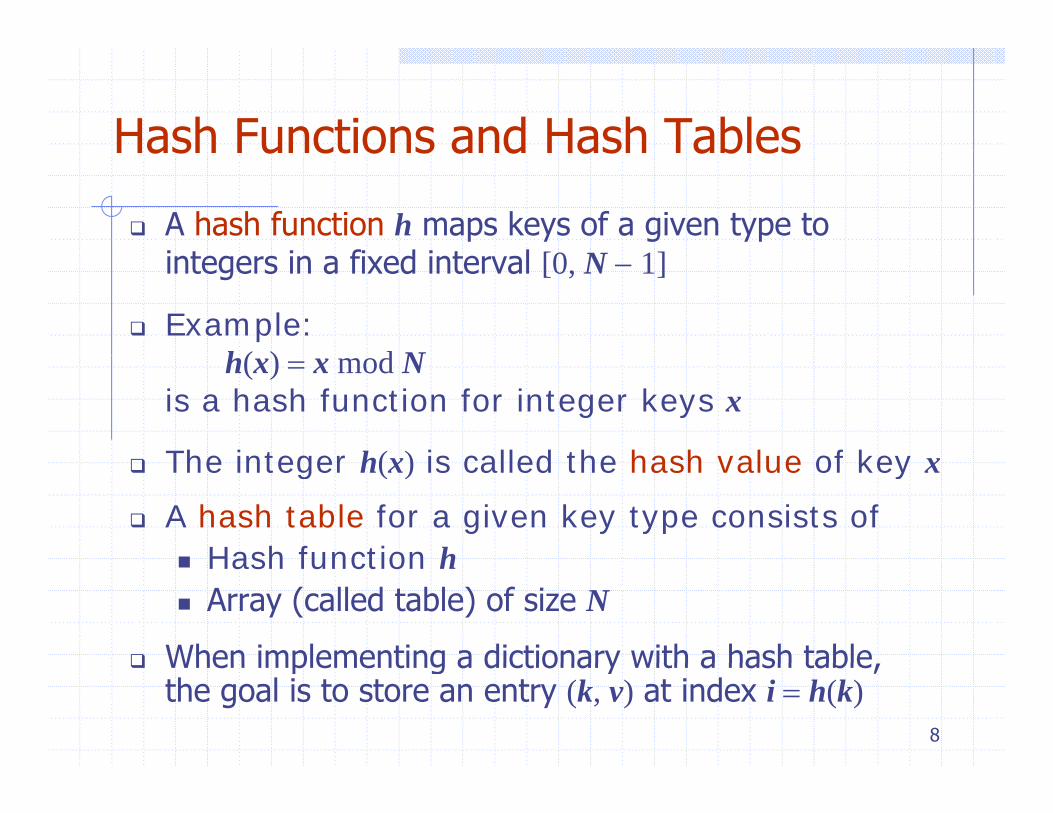
Hash Functions and Hash TablesHash Functions and Hash Tables

A hash function h maps keys of a given type to i t i fi d i t l [0 N 1]integers in a fixed interval [0, N − 1]

Example:h( ) d Nh(x) = x mod N

is a hash function for integer keys x

The integer h( ) is called the hash value of key The integer h(x) is called the hash value of key x

A hash table for a given key type consists ofHash function hHash function hArray (called table) of size N

When implementing a dictionary with a hash table

8

When implementing a dictionary with a hash table, the goal is to store an entry (k, v) at index i = h(k)

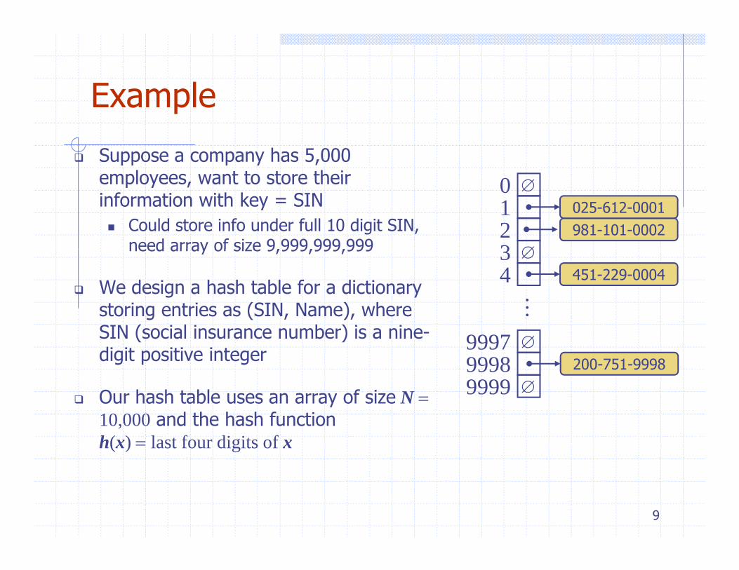
ExampleExample

Suppose a company has 5,000 employees want to store theiremployees, want to store their information with key = SIN

Could store info under full 10 digit SIN, need array of size 9,999,999,999

∅

∅

0123

981-101-0002025-612-0001

need array of size 9,999,999,999

We design a hash table for a dictionary storing entries as (SIN, Name), where

∅34 …

451-229-0004

SIN (social insurance number) is a nine-digit positive integer

O h h t bl f i N

∅

∅

999799989999

200-751-9998

Our hash table uses an array of size N = 10,000 and the hash functionh(x) = last four digits of x

9999

9

Hash Functions

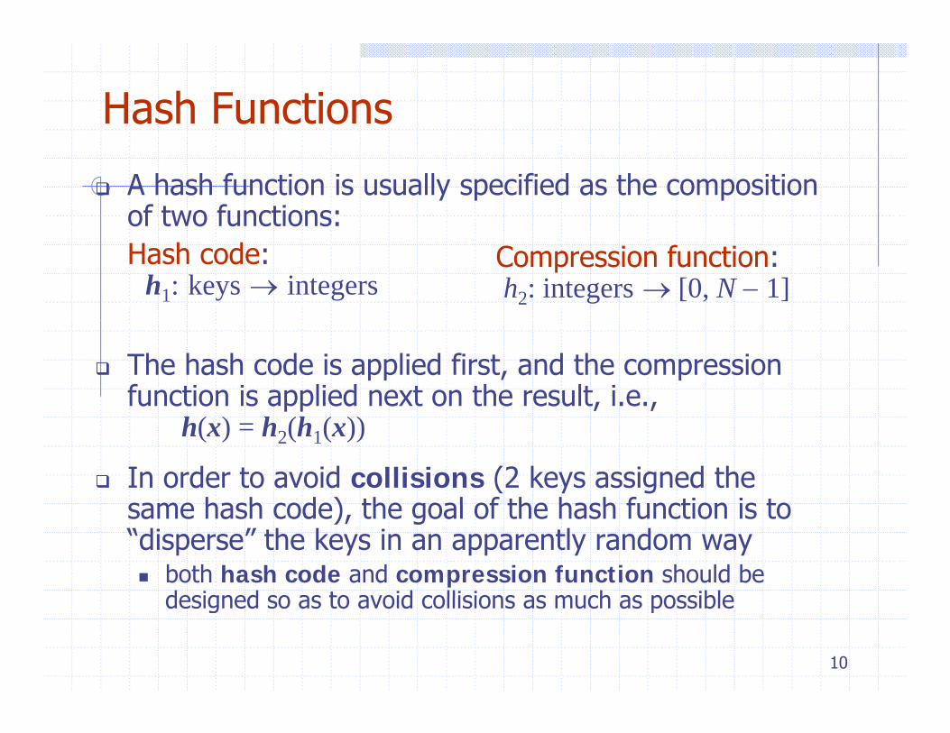
A hash function is usually specified as the composition of two functions:Hash code:

h1: keys → integersCompression function:h2: integers → [0, N − 1]

The hash code is applied first, and the compression function is applied next on the result, i.e.,

h(x) = h2(h1(x))

In order to avoid collisions (2 keys assigned the same hash code) the goal of the hash function is tosame hash code), the goal of the hash function is to “disperse” the keys in an apparently random way

both hash code and compression function should be designed so as to avoid collisions as much as possible

10

designed so as to avoid collisions as much as possible

Hash CodesHash CodesHash code maps a key k to an integer

Not necessarily in the desired range [0, …, N-1]May be even negative

We will assume a hash code is a 32-bit integer

Hash code should be designed to avoid collisions asHash code should be designed to avoid collisions as much as possible

If hash code causes collision, then compression function will not resolve this collisionnot resolve this collision

11

Hash Code Example 1: Memory Address

We can reinterpret the memory address of the key object as an integer

This is what is usually done in Java implementations any object inherits hashCode() method

May be sufficient, but we usually want “equal “ objects to have the same hash code, this will not happen with inherited hashCode() for example:inherited hashCode(), for example:

Want equal strings (“Hello” and “Hello”) to have the same hash code, however they will be stored at different memory locations, and will not have the same hashCode()

Want Integers with the same intValue() map to the same hash code but since they are stored at different memory locations

12

code, but since they are stored at different memory locations, they will not have the same hashCode()

Hash Code Example 2: Integer InterpretationHash Code Example 2: Integer Interpretation

We reinterpret the bits of the key as an integer

Suitable for keys of length less than or equal to the number of bits of the integer type

For byte, short, int, char, cast them into type int

For float, use Float.floatToIntBits()For float, use Float.floatToIntBits()

For 64-bit types long or double, if we cast them into int, half of the information is not used,

many collisions possible if the big difference between keys is in those lost bits

13

Hash Code Example 3: Component SumHash Code Example 3: Component Sum

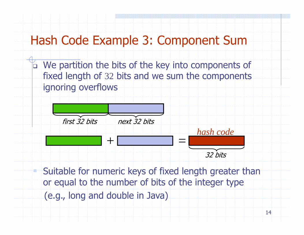
We partition the bits of the key into components of fi d l th f 32 bit d th tfixed length of 32 bits and we sum the components ignoring overflows

first 32 bits next 32 bitshash codehash code

+ =32 bits

Suitable for numeric keys of fixed length greater than or equal to the number of bits of the integer type

14

(e.g., long and double in Java)

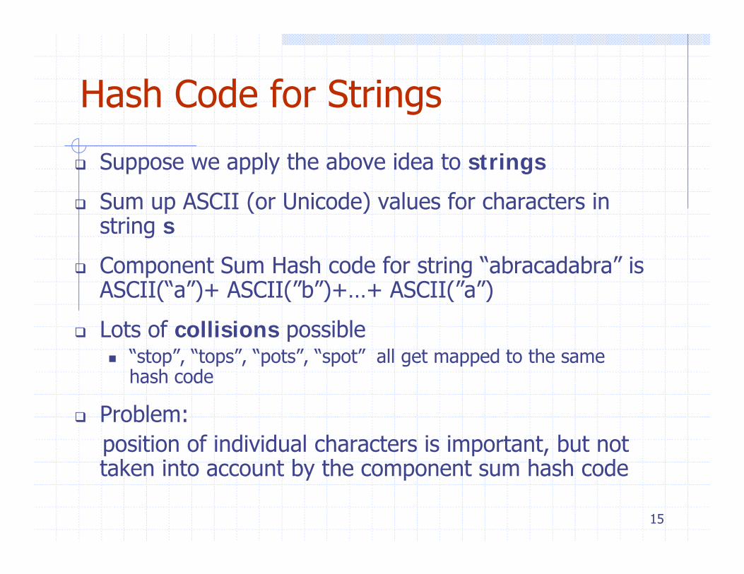
Hash Code for StringsHash Code for Strings

Suppose we apply the above idea to strings

Sum up ASCII (or Unicode) values for characters in string s

Component Sum Hash code for string “abracadabra” is ASCII(“a”)+ ASCII(”b”)+…+ ASCII(”a”)

L t f lli i iblLots of collisions possible“stop”, “tops”, “pots”, “spot” all get mapped to the same hash code

Problem: position of individual characters is important, but not taken into account by the component sum hash code

15

taken into account by the component sum hash code

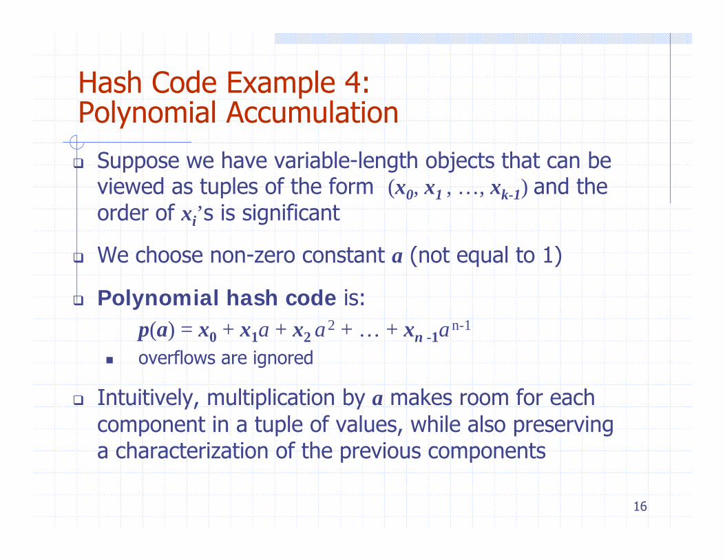
Hash Code Example 4: P l i l A l tiPolynomial Accumulation

Suppose we have variable-length objects that can be viewed as tuples of the form (x0, x1 , …, xk-1) and the order of xi’s is significant

We choose non-zero constant a (not equal to 1)

Polynomial hash code is:p(a) = x0 + x1a + x2 a2 + … + xn -1an-1

overflows are ignored

Intuitively, multiplication by a makes room for each component in a tuple of values, while also preserving a characterization of the previous components

16

a characterization of the previous components

Hash Code Example 4: Polynomial Accumulation

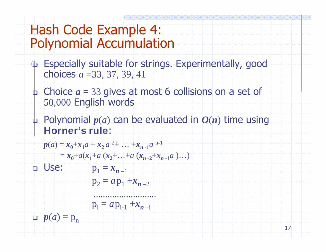
Especially suitable for strings. Experimentally, good choices a =33, 37, 39, 41

Polynomial Accumulation

, , ,

Choice a = 33 gives at most 6 collisions on a set of 50,000 English words

Polynomial p(a) can be evaluated in O(n) time using Horner’s rule:

( ) 2 n 1p(a) = x0+x1a + x2 a 2+ … +xn -1a n-1

= x0+a(x1+a (x2+…+a (xn -2+xn -1a )…)Use: p1 = xn –1

p2 = ap1 +xn –2

...........................pi = api 1 +x i

17

pi api-1 +xn –ip(a) = pn

Hash Code Example 4: Polynomial Accumulation

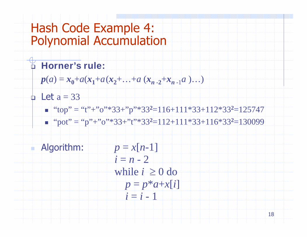
Horner’s rule:

Polynomial Accumulation

p(a) = x0+a(x1+a(x2+…+a (xn -2+xn -1a )…)

Let a = 33“top” = “t”+”o”*33+”p”*332=116+111*33+112*332=125747“pot” = “p”+”o”*33+”t”*332=112+111*33+116*332=130099

Algorithm: p = x[n-1]i = n - 2while i ≥ 0 do

p = p*a+x[i]i i 1

18

i = i - 1

Compression Functions p

Now know how to map objects to integers using it bl h h da suitable hash code

The hash code for key k will typically not in the legal range [0, …, N-1]

Need compression function to map the hash code into the legal range [0, …, N-1]

Good compression function will minimize the ppossible number of collisions

19

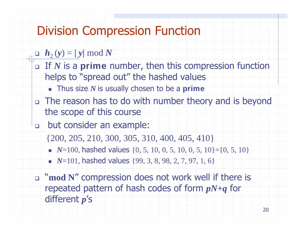
Division Compression Function

h2 (y) = | y| mod NIf N is a prime number, then this compression function helps to “spread out” the hashed values

Thus size N is usually chosen to be a prime

The reason has to do with number theory and is beyondThe reason has to do with number theory and is beyond the scope of this coursebut consider an example: {200, 205, 210, 300, 305, 310, 400, 405, 410}

N=100, hashed values {0, 5, 10, 0, 5, 10, 0, 5, 10}={0, 5, 10}N=101 hashed values {99 3 8 98 2 7 97 1 6}N=101, hashed values {99, 3, 8, 98, 2, 7, 97, 1, 6}

“mod N” compression does not work well if there is repeated pattern of hash codes of form pN+q for

20

repeated pattern of hash codes of form pN+q for different p’s

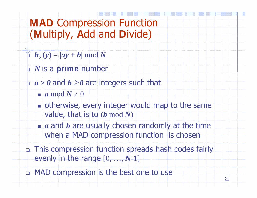
MAD Compression Function (Multiply, Add and Divide)(Multiply, Add and Divide)

h2 (y) = |ay + b| mod N

N is a prime number

a > 0 and b ≥ 0 are integers such thatga mod N ≠ 0otherwise, every integer would map to the same

l h ivalue, that is to (b mod N)a and b are usually chosen randomly at the time when a MAD compression function is chosenwhen a MAD compression function is chosen

This compression function spreads hash codes fairly evenly in the range [0, …, N-1]

21

y g [ , , ]

MAD compression is the best one to use

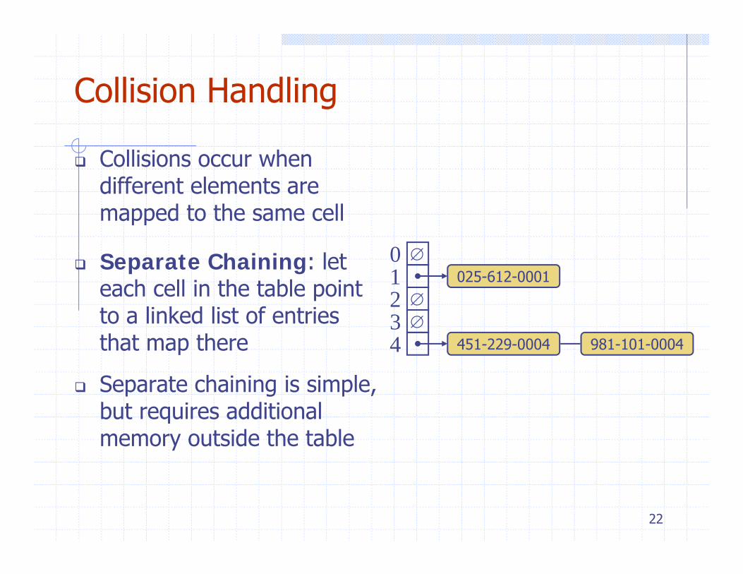
Collision Handlingg

Collisions occur when diff t l tdifferent elements are mapped to the same cell

∅0Separate Chaining: let each cell in the table point to a linked list of entries

∅

∅∅

0123

025-612-0001

to a linked list of entries that map there

Separate chaining is simple,

∅34 451-229-0004 981-101-0004

p g p ,but requires additional memory outside the table

22

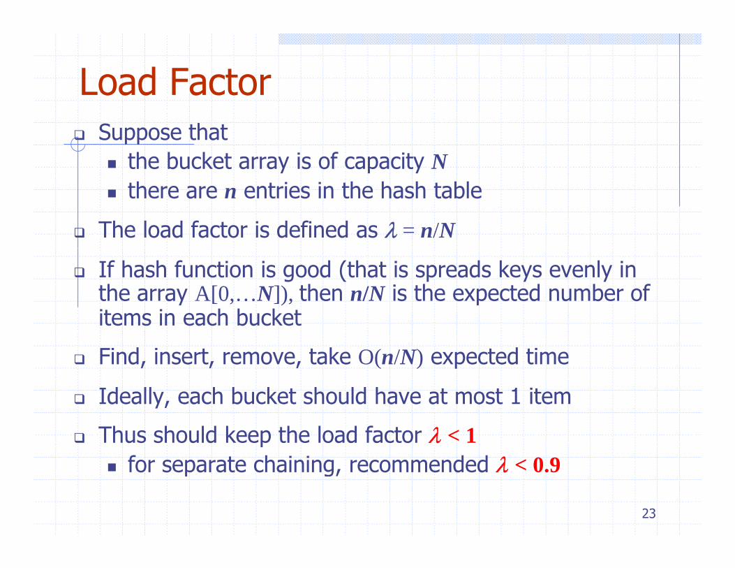
Load FactorSuppose that

the bucket array is of capacity Nthere are n entries in the hash table

The load factor is defined as λ = n/N

If hash function is good (that is spreads keys evenly in the array A[0,…N]), then n/N is the expected number of items in each bucketitems in each bucket

Find, insert, remove, take O(n/N) expected time

Ideall each b cket sho ld ha e at most 1 itemIdeally, each bucket should have at most 1 item

Thus should keep the load factor λ < 1for separate chaining recommended λ < 0 9

23

for separate chaining, recommended λ < 0.9

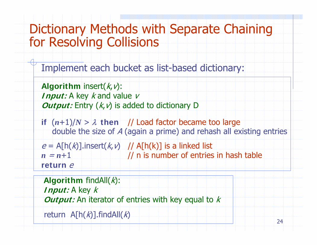
Dictionary Methods with Separate Chaining for Resolving Collisionsfor Resolving Collisions

Implement each bucket as list-based dictionary:

Algorithm insert(k,v):Input: A key k and value vOutput: Entry (k,v) is added to dictionary DOutput: Entry (k,v) is added to dictionary D

if (n+1)/N > λ then // Load factor became too largedouble the size of A (again a prime) and rehash all existing entries

e = A[h(k)].insert(k,v) // A[h(k)] is a linked list n = n+1 // n is number of entries in hash tablereturn e

Algorithm findAll(k):Input: A key kOutput: An iterator of entries with key equal to k

24

Output: An iterator of entries with key equal to k

return A[h(k)].findAll(k)

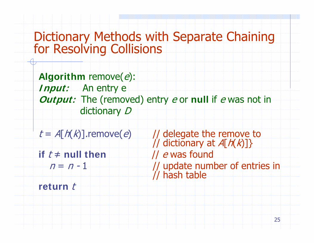
Dictionary Methods with Separate Chaining f R l i C lli ifor Resolving Collisions

Algorithm remove(e):Algorithm remove(e):Input: An entry eOutput: The (removed) entry e or null if e was not in

dictionary D

t = A[h(k)].remove(e) // delegate the remove tot A[h(k)].remove(e) // delegate the remove to // dictionary at A[h(k)]}

if t ≠ null then // e was foundn = n - 1 // update number of entries inn n 1 // update number of entries in

// hash tablereturn t

25

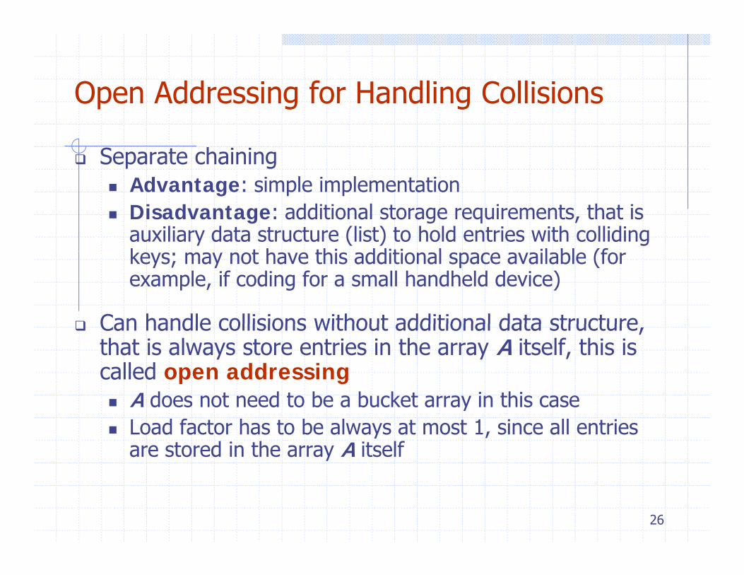
Open Addressing for Handling Collisionsp g g

Separate chainingAd t i l i l t tiAdvantage: simple implementationDisadvantage: additional storage requirements, that is auxiliary data structure (list) to hold entries with colliding k t h thi dditi l il bl (fkeys; may not have this additional space available (for example, if coding for a small handheld device)

Can handle collisions without additional data structureCan handle collisions without additional data structure, that is always store entries in the array A itself, this is called open addressing

A does not need to be a bucket array in this caseA does not need to be a bucket array in this caseLoad factor has to be always at most 1, since all entries are stored in the array A itself

26

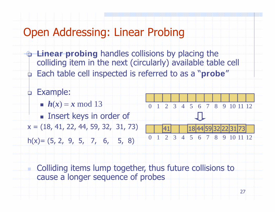
Open Addressing: Linear Probing

Linear probing handles collisions by placing the colliding item in the next (circularly) available table cellg ( y)Each table cell inspected is referred to as a “probe”

Example:Example:h(x) = x mod 13Insert keys in order of

0 1 2 3 4 5 6 7 8 9 10 11 12

yx = (18, 41, 22, 44, 59, 32, 31, 73)

h(x)= (5, 2, 9, 5, 7, 6, 5, 8) 0 1 2 3 4 5 6 7 8 9 10 11 1218 44 59 32 22 31 7341

Colliding items lump together, thus future collisions to

27

cause a longer sequence of probes

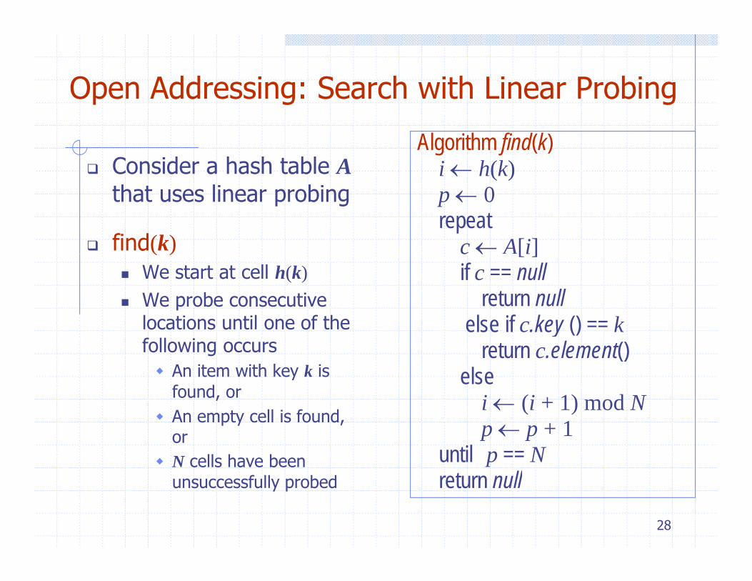
Open Addressing: Search with Linear Probing

Consider a hash table AAlgorithm find(k)

i ← h(k)that uses linear probing

find(k)

( )p ← 0repeat

c ← A[i]( )We start at cell h(k)We probe consecutive locations until one of the

c ← [i]if c == null

return nullelse if c key () == klocations until one of the

following occursAn item with key k is found, or

else if c.key () == kreturn c.element()

elsei ← (i + 1) mod N,

An empty cell is found, orN cells have been

i ← (i + 1) mod Np ← p + 1

until p == Nt ll

28

unsuccessfully probed return null

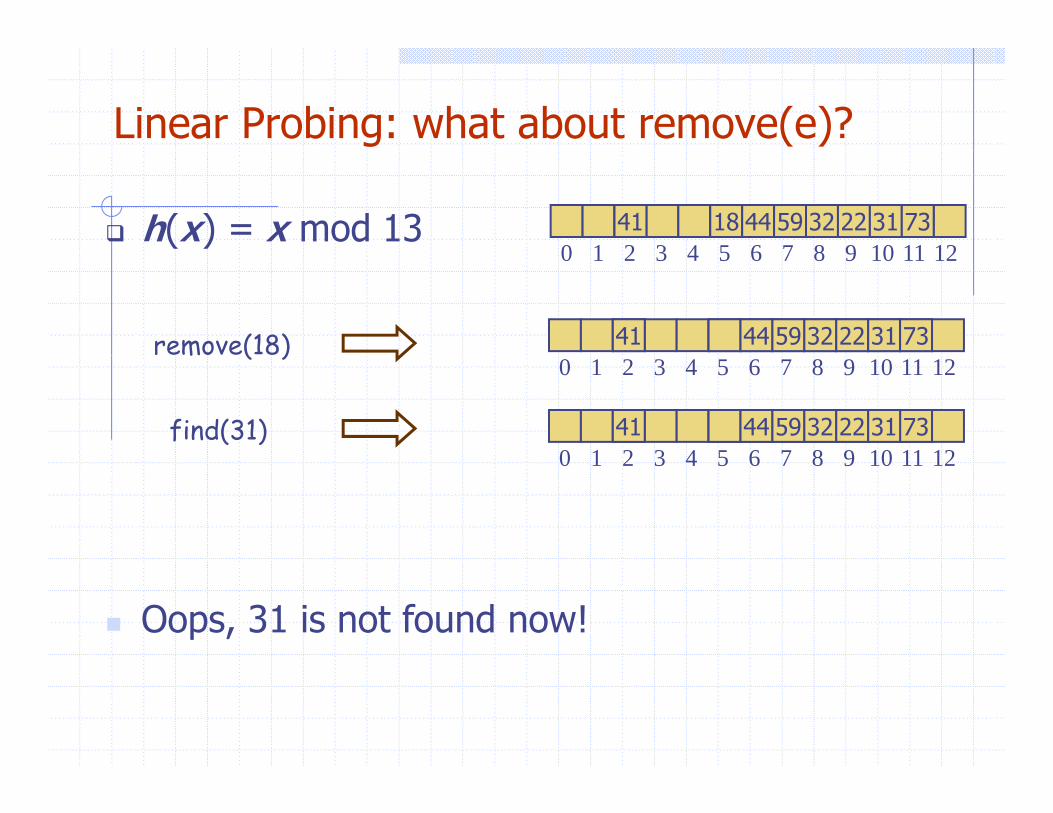
Linear Probing: what about remove(e)?

0 1 2 3 4 5 6 7 8 9 10 11 1218 44 59 32 22 31 7341h(x) = x mod 13

0 1 2 3 4 5 6 7 8 9 10 11 12

44 59 32 22 31 7341remove(18)0 1 2 3 4 5 6 7 8 9 10 11 12

0 1 2 3 4 5 6 7 8 9 10 11 1244 59 32 22 7341 31

m ( )

find(31)0 1 2 3 4 5 6 7 8 9 10 11 12

Oops, 31 is not found now!

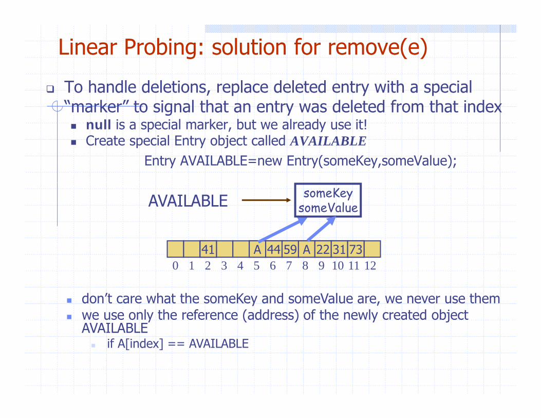
Linear Probing: solution for remove(e)

To handle deletions, replace deleted entry with a special “marker” to signal that an entry was deleted from that index

null is a special marker, but we already use it! p , yCreate special Entry object called AVAILABLE

Entry AVAILABLE=new Entry(someKey,someValue);

AVAILABLE someKeysomeValue

0 1 2 3 4 5 6 7 8 9 10 11 12A 44 59 A 22 31 7341

don’t care what the someKey and someValue are, we never use themwe use only the reference (address) of the newly created object AVAILABLE

if A[inde ] AVAILABLEif A[index] == AVAILABLE

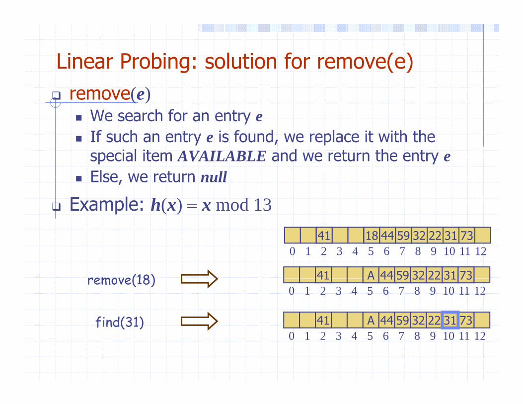
Linear Probing: solution for remove(e)remove(e)

We search for an entry eIf such an entry e is found, we replace it with the special item AVAILABLE and we return the entry eElse we return nullElse, we return null

Example: h(x) = x mod 13

0 1 2 3 4 5 6 7 8 9 10 11 1218 44 59 32 22 31 7341

A 44 59 32 22 31 7341remove(18)0 1 2 3 4 5 6 7 8 9 10 11 12

A 44 59 32 22 31 7341

A 44 59 32 22 7341 31

remove(18)

find(31)0 1 2 3 4 5 6 7 8 9 10 11 12

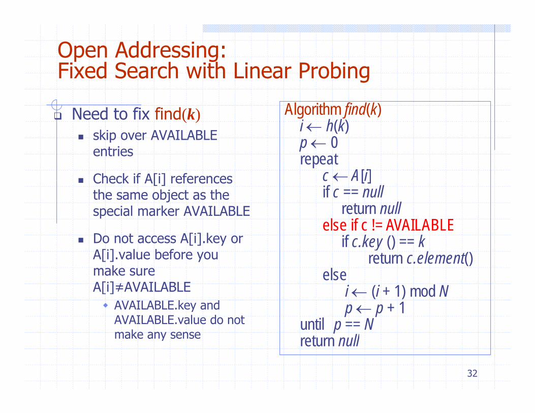
Open Addressing: Fixed Search with Linear ProbingFixed Search with Linear Probing

Need to fix find(k) Algorithm find(k)i ← h(k)

skip over AVAILABLE entries

Check if A[i] references

i ← h(k)p ← 0repeat

c ← A[i]Check if A[i] references the same object as the special marker AVAILABLE

c ← A[i]if c == null

return nullelse if c != AVAILABLE

Do not access A[i].key or A[i].value before you make sure A[i]≠AVAILABLE

if c.key () == kreturn c.element()

elseA[i]≠AVAILABLE

AVAILABLE.key and AVAILABLE.value do not make any sense

i ← (i + 1) mod Np ← p + 1

until p == Nt ll

32

make any sense return null

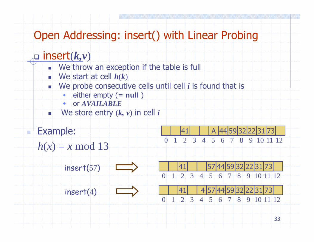
Open Addressing: insert() with Linear Probing

insert(k,v)We throw an exception if the table is fullWe start at cell h(k)We start at cell h(k) We probe consecutive cells until cell i is found that is

either empty (= null )or AVAILABLEor AVAILABLE

We store entry (k, v) in cell i

Example: A 44 59 32 22 7341 31

h(x) = x mod 13 0 1 2 3 4 5 6 7 8 9 10 11 12

57 44 59 32 22 31 7341insert(57)0 1 2 3 4 5 6 7 8 9 10 11 12

57 44 59 32 22 31 7341insert(57)

insert(4) 40 1 2 3 4 5 6 7 8 9 10 11 12

57 44 59 32 22 31 7341

33

0 1 2 3 4 5 6 7 8 9 10 11 12

Open Addressing: Updates with Linear ProbingUpdates with Linear Probing

Disadvantages of Linear Probingg g

code is more complicated

entries tend to cluster into contiguous runs, which g ,slows down the find and insert operations significantly

34

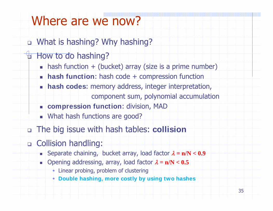
Where are we now?

Wh t i h hi ? Wh h hi ?What is hashing? Why hashing?

How to do hashing?hash function + (bucket) array (size is a prime number)hash function + (bucket) array (size is a prime number)hash function: hash code + compression functionhash codes: memory address, integer interpretation,

component sum, polynomial accumulationcompression function: division, MAD What hash functions are good?g

The big issue with hash tables: collision

Collision handling:Collision handling:Separate chaining, bucket array, load factor λ = n/N < 0.9Opening addressing, array, load factor λ = n/N < 0.5

Linear probing, problem of clustering

35

Linear probing, problem of clusteringDouble hashing, more costly by using two hashes

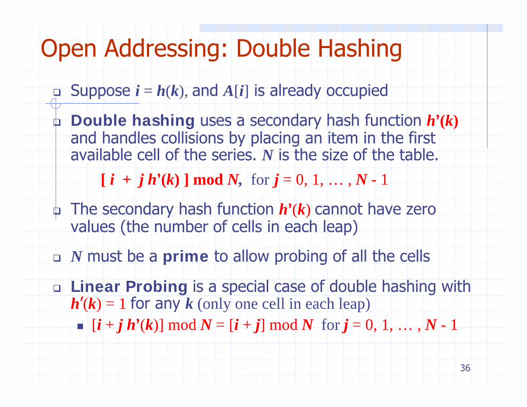
Open Addressing: Double Hashing

Suppose i = h(k), and A[i] is already occupied

Double hashing uses a secondary hash function h’(k) g y ( )and handles collisions by placing an item in the first available cell of the series. N is the size of the table.

[ i + j h’(k) ] mod N for j = 0 1 N 1[ i + j h (k) ] mod N, for j = 0, 1, … , N - 1

The secondary hash function h’(k) cannot have zero values (the number of cells in each leap)values (the number of cells in each leap)

N must be a prime to allow probing of all the cells

Li P bi i i l f d bl h hi i hLinear Probing is a special case of double hashing with h’(k) = 1 for any k (only one cell in each leap)

[i + j h’(k)] mod N = [i + j] mod N for j = 0, 1, … , N - 1

36

[ j ( )] [ j] j , , ,

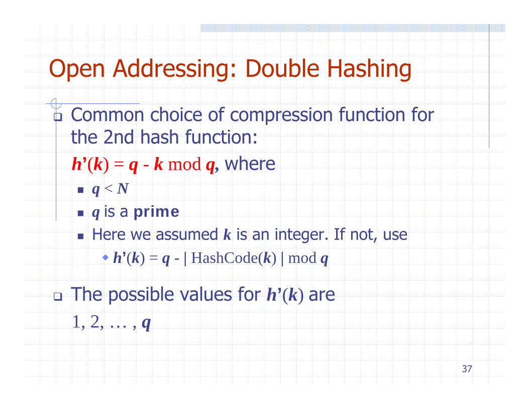
Open Addressing: Double HashingOpen Addressing: Double Hashing

Common choice of compression function for the 2nd hash function: h’(k) = q - k mod q, where

q < Nq is a primeH d k i i t If tHere we assumed k is an integer. If not, use

h’(k) = q - | HashCode(k) | mod q

The possible values for h’(k) are1, 2, … , q

37

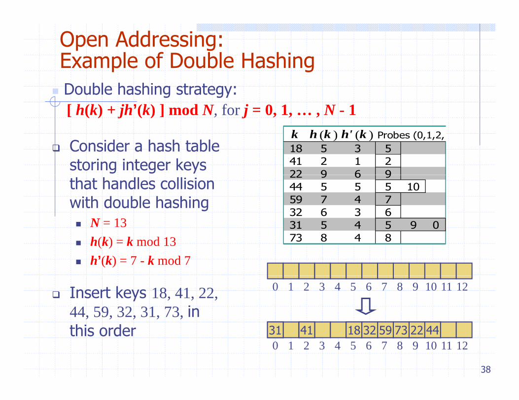
Open Addressing: Example of Double HashingDouble hashing strategy: [ h(k) + jh’(k) ] mod N, for j = 0, 1, … , N - 1

Consider a hash table storing integer keys

k h (k ) h' (k ) Probes (0,1,2,…18 5 3 541 2 1 222 9 6 9

that handles collision with double hashing

N = 13

22 9 6 944 5 5 5 1059 7 4 732 6 3 631 5 4 5 9 0N 13

h(k) = k mod 13 h’(k) = 7 - k mod 7

31 5 4 5 9 073 8 4 8

Insert keys 18, 41, 22, 44, 59, 32, 31, 73, in thi d

0 1 2 3 4 5 6 7 8 9 10 11 12

1841 22 44593231 73

38

this order0 1 2 3 4 5 6 7 8 9 10 11 12

1841 22 44593231 73

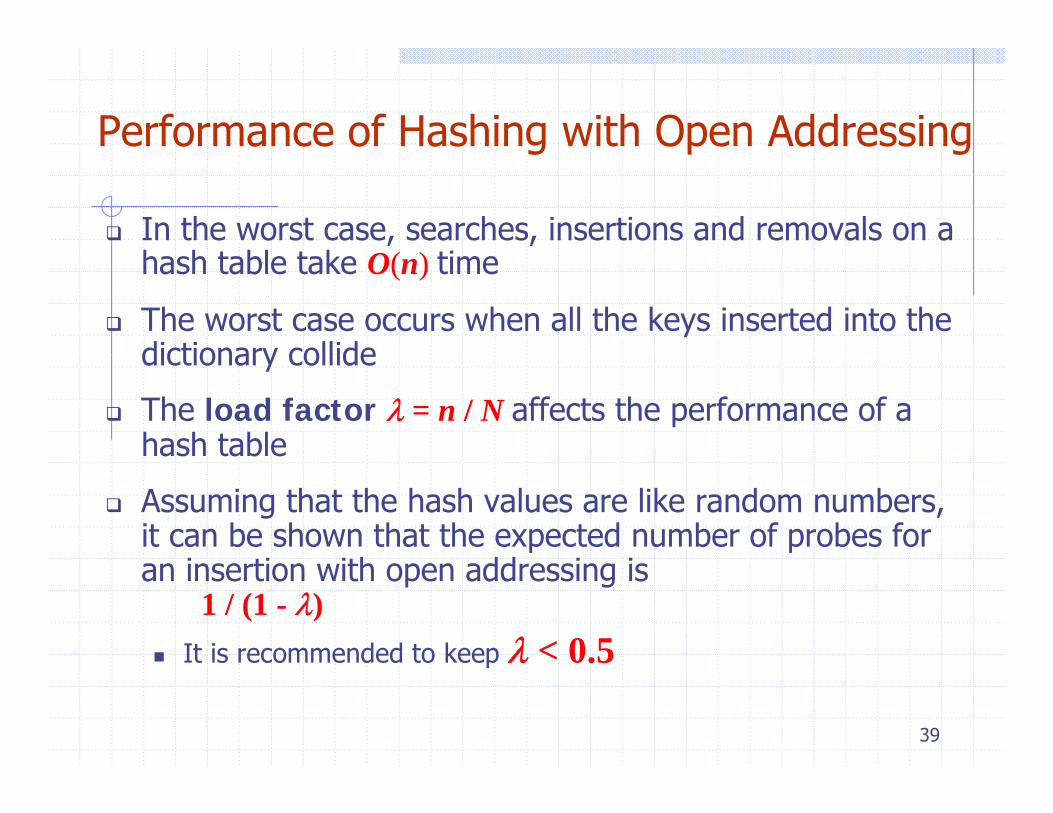
Performance of Hashing with Open Addressingg p g

In the worst case, searches, insertions and removals on a h h t bl t k O( ) tihash table take O(n) time

The worst case occurs when all the keys inserted into the dictionary collidedictionary collide

The load factor λ = n / N affects the performance of a hash table

Assuming that the hash values are like random numbers, it can be shown that the expected number of probes for

i ti ith dd i ian insertion with open addressing is1 / (1 - λ)

It is recommended to keep λ < 0.5

39

p 0 5

Separate Chaining vs. Open AddressingSeparate Chaining vs. Open Addressing

Open addressing saves space over separate chainingOpen addressing saves space over separate chaining

Separate chaining is usually faster (depending on load factor of the bucket array) than openload factor of the bucket array) than open addressing, both theoretically and experimentally

Thus if memory space is not a major issue useThus, if memory space is not a major issue, use separate chaining, otherwise use open addressing

40

Performance of HashingPerformance of Hashing

The expected running time of all the dictionary ADT operations in a hash table is O(1)

In practice, hashing is very fast provided the load factor is not close to 1

Rehash with bigger array if load factor becomes badRule of thumb: new array twice the size of old array (still a prime)

Applications of hash tables:small databasescompilersweb browser caches

41