1

Has the Correlation of Inflation and Stock Prices Changed in the

United States over the Last Two Centuries? *

Nikolaos Antonakakis*

* Corresponding author. University of Portsmouth, Economics and Finance Subject Group,

Portsmouth Business School, Portland Street, Portsmouth, PO1 3DE, United Kingdom.

nikolaos.antonakakis@port.ac.uk

Webster Vienna Private University, Department of Business and Management, Praterstrasse 23, 1020,

Vienna, Austria. Nikolaos.antonakakis@webster.ac.at

Rangan Gupta

Department of Economics, Faculty of Economic and Management Sciences, University of Pretoria, 0002,

South Africa

Aviral K. Tiwari

Faculty of Management, IBS Hyderabad, IFHE University, Donthanapally Shankarapalli Road,

Hyderabad, Andhra Pradesh 501203, India

Abstract

The relationship between stock prices and the inflation can be either negative or positive,

depending on the strengths of various theoretical channels at work. In this study, we examine the

dynamic conditional correlations of stock prices and inflation in the United States over the period

of 1791-2015 under a time-varying framework. The results of our empirical analysis reveal that

correlations between the inflation and stock prices in the United States evolve heterogeneously

overtime. In particular, the correlations are significantly positive in the 1840s, 1860s, 1930s and

2011, and significantly negative otherwise. The policy implications of these findings are then

discussed.

Keywords: Conditional correlation, GARCH, Inflation and Stock Price Comovement, US

Economy

JEL codes: C32, C50, E31, E44, G1, N1

* We would like to thank the editor (T. Lagoarde Segot) and an anonymous referee for many helpful comments and

suggestions on a previous version of this paper. The usual disclaimer applies.

2

1. Introduction

Stock prices are considered to be a leading indicator for economic activity of the U.S. economy

(Stock and Watson, 2003; Rapach and Weber, 2004), and hence, determining what factors drive

this market is of paramount importance. While stock prices are primarily driven by financial

variables (Valcarcel, 2012), the importance of macroeconomic variables cannot be ruled out either

(Goyal and Welch, 2008; Valcarcel, 2012, Rapach and Zhou, 2013). Inflation is undoubtedly one

of the most important macroeconomic variables believed to be related to stock prices, and in turn,

also affected by it (Gupta and Inglesi-Lotz, 2012).

While inflationary shocks may have little long-run impact on real stock returns, due to monetary

non-neutrality, it is generally agreed that stock prices can be affected by inflation in the short-run

(Rapach, 2002; Bjørnland and Leitemo, 2009; Valcarcel, 2012; Bjørnland and Jacobsen, 2013).

In this regard, there are many channels through which inflation can affect stock prices, with the

effect being either positive or negative depending upon the theory in consideration. The Gordon

(1962) growth model shows that stock prices are directly related to current and expected growth

rates of dividend returns and inversely related to the required rate of return on the equity. Given

this, inflation has a positive impact on stock prices through two channels: First, a monetary easing

that stimulates the economy along with inflation would have a positive impact on the growth rate

of dividends. Second, a monetary expansion that depresses bond returns would result in an

increased demand for equities, which in turn, would cause the average investor to lower expected

rate of returns of equities. Whether it is increased dividend returns or decreased expected returns

on investment, both serve to raise stock prices. The possibility of inflation leading to lower stock

returns also has multiple explanations. First, as discussed in Modigliani and Cohn (1979), agents

could discount asset valuations at an artificially high rate in the presence of sustained inflation, as

it is difficult to distinguish between real and nominal returns when the latter includes an inflation

premium. Second, Feldstein (1980) points out that sustained increases in inflation reduces real

stock prices since the tax code exerts a distortionary effect between depreciation costs and capital

gains. Third, Fama (1981), based on his proxy-effect hypothesis (PEH), believes that the negative

correlation is induced by a positive relationship between stock returns and expected economic

activity (as proxied by inflation) and an inverse relationship between expected economic activity

and inflation. Finally, as pointed out by Sargent (1999), and Cogley and Sargent (2001), if the

3

monetary authority, under the assumption of an exploitable trade-off between inflation and

unemployment, succumbs to the temptation to inflate (until time-consistent inflation rates are

achieved), the resulting higher expectations of inflation would increase long-term rates leading

investors to more aggressively discount future dividends (Valcarcel, 2012). At the same time, the

subsequent contractionary monetary policy actions could also contribute to lower stock returns

due to slowing down of economic activity and, thus, depressing current and expected future

earnings (Valcarcel, 2012). Hence, theoretically, inflation can either increase or decrease stock

prices.

At the same time, real stock price movements can affect the inflation rate through the wealth-

effect, i.e., via its impact on consumption and hence aggregate demand. Ludwig and Sløk (2004),

and more recently Simo-Kengne et al., (2015), discusses four different channels of influence for

stock prices on consumption: First, the realised wealth effect implies that an increase in stock

prices exerts a direct positive effect on stockholders’ consumption as a consequence of the realised

gain. Second, the unrealised wealth effect refers to the increase in consumption spending based on

the expectation that raising the current stock price will result in higher future income and wealth.

Third, the liquidity constraint effect implies that increasing stock prices raise the value of collateral

against which financially constraint households may borrow to increase their consumption. Fourth,

the stock option value effect, implies that an increase in stock prices leads to the increase in the

value of stockholders options which may translate into higher consumption irrespective of whether

the gains are realised or unrealised. In other words, real stock prices and inflation is likely to be

positively related through the wealth effect.

Against this backdrop, the objective of our study is to analyse the evolution of the correlation

between real stock price and inflation for the US economy using Engle (2002) dynamic conditional

correlation (DCC)-GARCH model on annual data over the period of 1791-2015. As discussed

above, the relationship between real stock prices (returns) and inflation is contingent upon the

strength of the various channels at a specific point in time or over a certain period. Hence, there is

a need to pursue a time-varying approach especially when we account for the long-span of data

under investigation. Similar thoughts were also echoed in the works of Durham (2003) and He

(2006). Besides accounting for time-varying conditional volatility behaviour of data (given the

4

abundant empirical evidence of a substantial decline in the volatility of most US macroeconomic

aggregates (Valcarcel, 2012)), a major advantage of the DCC-GARCH approach is its ability to

detect changes in the conditional correlation over time. Moreover, it is able to distinguish negative

correlations due to episodes in single years, synchronous behavior during stable years and

asynchronous behavior in turbulent years. Unlike rolling windows, an alternative way to capture

time variability, the proposed measure does not suffer from the so-called “ghost features”, as the

effects of a shock are not reflected in n consecutive periods, with n being the window span. In

addition, under the proposed measure there is neither a need to set a window span, nor loss of

observations, nor subsample estimation required.

As discussed above, contingent on the signs of the channels at work, the relationship between real

stock price and inflation could be either negative or positive, as also highlighted by Valcarcel

(2012). Hence, it is important to pursue a time-varying approach for analyzing the conditional

comovement between these variables to check the evolution of this relationship. The DCC-

GARCH approach allows us to check if, in fact the relationship is indeed time-varying (state-

contingent) or not, besides the nature of the relationship itself.

A constant parameter approach, as has been primarily applied so far in the literature (see for

example Hess and Lee, 1999; Rapach, 2001; Binswanger, 2004; He, 2006; Lee, 2010; Gupta and

Inglesi-Lotz, 2012; Valcarcel, 2012; and references cited there in for detailed literature reviews),

based on an average value of the correlation estimate, which is generally negative, is likely to be

misleading in terms of policy, as it will not allow the policy maker to deduce the importance of

the various effects that drive this relationship at specific points in time. To the best of our

knowledge, Valcarcel (2012) is the only paper that has used a time-varying Vector Autoregressive

(VAR) model to analyze the relationship between real stock returns and inflation for the US

economy over the quarterly period of 1955:1 to 2011:2. So, in this regard, our paper can be

considered to be an extension of the work of Valcarcel (2012) by considering the longest possible

sample period spanning over two centuries of annual data tracking the history of U.S. inflation in

relationship to stock prices. In addition, we also check whether our results are robust to data

frequency using a monthly data set of real stock returns and inflation spanning nearly 150 years

(1871-2015).

5

At this stage, it is important to indicate the reasons behind our preference to use a DCC-GARCH

approach rather than a time-varying VAR method. First, as is well-known, identifying shocks in a

VAR would require us to order the real stock returns and inflation. However, at an annual

frequency, it is difficult to postulate which variable can be ordered first i.e., believed to be more

exogenous. Of course, one could reverse the ordering and check for the robustness of the results.

But then again, this would not guard against the possibility that the degree of exogeneity over such

a long-span of data did not vary over time. An alternative approach would have been to use sign-

restricted time-varying VAR, but this would take away from us the very essence of our exercise

of deciphering the correlation between these two variables, which as indicated above could be

either positive or negative. In other words, one could not have without doubt imposed a theory-

based sign either. Keeping these issues in mind, we decided to resort to a DCC-GARCH approach,

which provides us with a time-varying correlation between these two variables accounting for

heteroscedastic disturbances, without having to worry about the ordering of variables or sign-

restrictions in a VAR model. Having said this, one limitation of our approach, given the long-span

of data, is our inability to control for other important variables (like interest rate, output and

or/unemployment) which are likely to affect both inflation and stock prices. In such a multivariate

setting, a VAR approach as used by Valcarcel (2012) is preferable, as it also allows us to analyze

the importance of the other variables (shocks) in the relationship between stock prices and

inflation. Nevertheless, given that our concern is a time-varying analysis of correlation between

these two variables, the DCC-GARCH framework can be considered most appropriate in our

context.

Our empirical results reveal that correlations between inflation and stock market returns are indeed

evolving heterogeneously overtime. In particular, the correlations are significantly positive in the

1840s, 1860s, 1930s and 2011, and significantly negative otherwise, indicating the time-varying

role relating the stock market with inflation in the U.S. Our main results based on annual data do

not suffer from time aggregation bias, as employing a shorter monthly dataset between January

1871 and October 2015 leads to very similar conclusions.

6

The remainder of the paper is organized as follows: Section 2 describes the empirical methodology,

while Section 3 the data used. Section 4 presents the empirical findings. Finally, Section 5

summarises the results, discusses their policy implications and offers some concluding remarks.

2. Methodology

In order to examine the evolution of co-movements between inflation and stock market returns,

we obtain a time-varying measure of correlation based on the dynamic conditional correlation

(DCC) model of Engle (2002).

Let 𝑦𝑡 = [𝑦1𝑡, 𝑦2𝑡]′ be a 2 × 1 vector comprising the data series (i.e. inflation and real stock market

returns). The conditional mean equations are then represented by

𝐴(𝐿)𝑦𝑡 = 𝜀𝑡, 𝑤ℎ𝑒𝑟𝑒 𝜀𝑡|Ω𝑡−1~𝑁(0, 𝐻𝑡), 𝑎𝑛𝑑 𝑡 = 1, . . . , 𝑇 (1)

where 𝐴 is a matrix of endogenous variables, 𝐿 the lag operator and 𝜀𝑡 is the vector of innovations

based on the information set, Ω, available at time 𝑡 − 1. The 𝜀𝑡 vector has the following conditional

variance-covariance matrix

𝐻𝑡 = 𝐷𝑡𝑅𝑡𝐷𝑡, (2)

where 𝐷𝑡 = 𝑑𝑖𝑎𝑔√ℎ𝑖𝑡 is a 2 × 2 matrix containing the time-varying standard deviations obtained

from univariate GARCH(p,q) models as

ℎ𝑖𝑡 = 𝛾𝑖 + ∑𝑃𝑖𝑝=1 𝛼𝑖𝑝𝜀𝑖𝑡−𝑖𝑝

2 + ∑𝑄𝑖𝑞=1 𝛽𝑖𝑞ℎ𝑖𝑞−𝑞, ∀𝑖 = 1,2. (3)

7

The DCC(M,N) model of Engle (2002) comprises the following structure

𝑅𝑡 = 𝑄𝑡∗−1Q𝑡𝑄𝑡

∗−1, (4)

where

𝑄𝑡 = (1 − ∑𝑀𝑚=1 𝑎𝑚 − ∑𝑁

𝑛=1 𝑏𝑛)�̅� + ∑𝑀𝑚=1 𝑎𝑚(𝜀𝑡−𝑚

2 ) + ∑𝑁𝑛=1 𝑏𝑛𝑄𝑡−𝑛. (5)

�̅� is the time-invariant variance-covariance matrix retrieved from estimating equation (3), and 𝑄𝑡∗

is a 2×2 diagonal matrix comprising the square root of the diagonal elements of 𝑄𝑡. Finally, 𝑅𝑡 =

𝜌𝑖𝑗𝑡=

𝑞𝑖𝑗,𝑡

√𝑞𝑖𝑖,𝑡𝑞𝑗𝑗,𝑡 where 𝑖, 𝑗 = 1,2 is the 2 × 2 matrix consisting of the conditional correlations

between inflation and stock market returns, and which are our main focus.

3. Data

The two main variables of interest in this paper are inflation and the stock market prices in the US

over the period of 1791-2015, i.e., 225 observations. Inflation, 𝐼𝑁𝐹, is measured as the difference

of the natural logarithm of the consumer price index (CPI), and stock market prices are measured

in real terms, i.e. deflated by the consumer price index (CPI) and then converted in real stock

market returns, 𝑅𝑆𝑅, by taking the first difference of the natural logarithm of real stock prices, so

as to render the series stationary. The CPI data comes from the website of Professor Robert Sahr.1

The nominal S&P500 stock price, which is deflated by the consumer price index (CPI) to get the

real S&P500, is obtained from the Global Financial Database.

1 http://liberalarts.oregonstate.edu/spp/polisci/research/inflation-conversion-factors-convert-dollars-1774-estimated-

2024-dollars-recent-year.

8

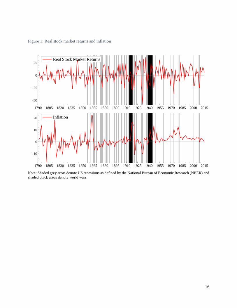
Figure 1 presents the evolution of inflation and real stock market returns.2 We can make the

following observations from the data plots: (a) Real stock returns, not surprisingly, fluctuates a lot

more than inflation over the entire sample period, given the volatile nature of the equity market in

general. Sharp declines were observed during the banking panics in the early part of 1800, US

Civil War, World War I, the “Great Depression”, World War II, the collapse of the Bretton Woods

agreement followed by the “Nixon Shock” (i.e., unilateral cancellation of the direct international

convertibility of the United States dollar to gold) and United States dollar devaluation under the

Smithsonian Agreement, the NASDAQ and Dotcom bubble crashes, and finally more recently due

to the recent global financial crisis originating from the subprime mortgage market; (b) Large

swings in the inflation rate can be observed in the early part of the sample, with the sharp increases

corresponding to the American Revolution, the creation of the United States mint with dollar

pegged to silver and gold, and the various wars such at the Franco-American Naval War, Barbary

Wars, War of 1812, Mexican War, Civil War, Spanish-American War, World War I and II, Korean

War, Vietnam War, and then of course, the creation of the Bretton Woods and dollar freely floating

with gold standard abandoned completely; oil shocks of the 1970s, and the so-called period of the

“Great Inflation” that lasted till around 1982 due to the excess growth in US money supply with

the aim to achieve full-employment believing the existence of the Phillips curve, after which it

came down to single figures following the so-called “Volcker-Disinflation”. Some inflationary

episodes were later observed during the Gulf-War and the Iraq War, with inflation declining during

the “Great Recession” and then picking up due to the quantitative easing policies of the Federal

Reserve. The early deflationary episode was associated with paper money being issued without

the backing of precious metals, Banking Panics in the early 1800s, and then in the aftermath of the

World War I followed by the “Great Depression” and partial abandoning of the Gold standard in

the 1930s.

[Insert Figure 1 around here]

2 The discussion here on stock markets is derived from:

https://www.nyse.com/publicdocs/American_Stock_Exchange_Historical_Timeline.pdf, while that on inflation

comes from: http://blogs.wsj.com/economics/2015/12/14/a-brief-history-of-u-s-inflation-since-1775/.

9

Table 1 presents the descriptive statistics of our data. According to this table, we observe large

variability in our main variables, especially of the stock market returns. Over the last 225 years,

the stock market in the United States has generated on average positive real returns equal to 1.58%,

while inflation was on average 1.44%. The augmented Dickey-Fuller (ADF) test with just a

constant indicates that both series are stationary. The fact that the ARCH-LM test rejects the null

hypothesis of homoskedasticity for each series indicates the appropriateness of modelling our

series as an ARCH-type process. Finally, the unconditional correlation between the trade balance

and real stock market returns, which is presented in the lower panel of Table 1, is negative and

equal to -0.2284.

[Insert Table 1 around here]

4. Estimation Results

Table 2 reports the results of the DCC model. Panels A and B present the conditional mean and

variance results, respectively, while Panel C contains the Ljung-Box Q-Statistics on the

standardized and squared standardized residuals up to 10 lags. The choice of the lag-length of the

autoregressive process of the conditional mean, which is equal to one, is based on the Akaike

information criterion (AIC) and Schwarz Bayesian criterion (BIC).

[Insert Table 2 around here]

According to the conditional mean results reported in Table 2, we find that past real stock market

returns are associated with significant increases in the current real stock market returns and

inflation, while past inflation is associated with increased current inflation and reduced current real

stock market returns.

The conditional variance results reported in the same table support the existence of the GARCH

effects found in the series, as the coefficients 𝛼1 and 𝛽1 are highly significant. Moreover, the

coefficients 𝑎 and 𝑏 are highly significant indicating that the correlations between inflation and

real stock market returns are indeed time-varying. Both these results validate the choice of the

10

DCC model. Finally, the model does not suffer from serial correlation in the squared (standardized)

residuals, according to the misspecification tests reported in Panel C of Table 2.

In Figure 2, we present the dynamic conditional correlations of inflation and real stock market

returns from the model in Table 2, along with their 90% confidence intervals. According to this

figure, it is evident that dynamic conditional correlations between inflation and real stock market

returns have behaved rather heterogeneously overtime. In particular, correlations are significantly

positive in the 1840s, 1860s, 1930s and 2011, and significantly negative otherwise (with the result

being in line with Valcarcel (2012) for the post-1960 period), indicating the time-varying role

relating the stock market with inflation in the U.S.3 If we look at Figure 1, then one would realize

that these are periods associated with the banking panics of early 1800s as discussed above, as well

as periods of major or post-recessions for the US economy, with negative real returns on stock

prices. These periods are also associated with major deflation, and with real stock returns

declining, implied that nominal stock returns declined proportionately more, which in turn, is

indicative of weakness in the financial market during these periods. This is not surprising given

that, we are talking of periods of the banking panics, the Great Depression, and the post-recent

financial crisis – all events that would lead to deterioration in the confidence of investors to invest

in the equity market. Understandably, lower stock returns could have resulted in lower

consumption, and hence weaker aggregate demand and thus lower rates of inflation through the

wealth effect as outlined above. Recall that, the realised wealth effect implies that a decrease in

stock prices exerts a direct negative effect on stockholders’ consumption as a consequence of the

realised loss. In addition, the unrealised wealth effect would suggest a fall in consumption

spending based on the expectation that declining stock prices will continue and cause lower future

income and wealth. Furthermore, the liquidity constraint effect would imply that decreases in stock

prices would lower the value of collateral against which would prevent financially constraint

households from borrowing, thus affecting their consumption. Finally, the stock option value

effect, implies that a decrease in stock prices leads to the decrease in the value of stockholders

options which may translate into lower consumption irrespective of whether the gains are realised

3 When we used nominal stock returns instead of real stock returns, we obtained similar correlation patterns over the

sample. Complete details of these results are available upon request from the authors.

11

or unrealised. So, all these effects put together, is likely to translate into lower aggregate demand

and lower inflation or deflation, which in turn leads to the positive correlation observed.

Alternatively, the Gordon (1962) growth model could be at work as well, which, in turn posits a

positive relationship between inflation and stock returns. These being periods of deflation and

recession, which in turn, could have resulted from a monetary contraction, would have a negative

impact on the growth rate of dividends. Also, a monetary contraction that increases bond returns

would result in a lower demand for equities, which in turn, would cause the average investor to

increase expected rate of returns of equities. Whether it is decreased dividend returns or increased

expected returns on investment, both serve to put reduce stock prices.

For the remainder of the periods, which are associated with calmer episodes of the US economy

characterized by steady growth and inflation, leading to lower stock returns could be due to: (a)

agents might be discounting asset valuations at an artificially high rate in the presence of sustained

inflation, as it is difficult to distinguish between real and nominal returns when the latter includes

an inflation premium; (b) Sustained increases in inflation reduces real stock prices since the tax

code exerts a distortionary effect between depreciation costs and capital gains; (c) The negative

correlation is induced by a positive relationship between stock returns and expected economic

activity (as proxied by inflation) and an inverse relationship between expected economic activity

and inflation, and; (d) If the monetary authority, believes in the Phillips curve, then it is likely to

succumb to the temptation to inflate, and the resulting higher expectations of inflation would

increase long-term rates leading investors to more aggressively discount future dividends. This last

explanation is quite well-accepted for the reason behind the inflationary episode observed in the

US following World War II, as indicated above while discussing Figure 1.

So overall, our result are in line with the historical episodes and events associated with the stock

and the macroeconomy in general, which in turn, have caused various channels to be at work at

different points in time.

[Insert Figure 2 around here]

12

4.1. Robustness analysis

As a robustness check, we examine whether our dynamic conditional correlation results of

inflation and real stock market returns based on annual data suffer from time aggregation bias. In

particular, we employ a monthly dataset between inflation and real stock market returns over the

period January 1871 to November 2015 (i.e. 1739 monthly observations) obtained from the online

data segment of Professor Robert J. Shiller.4 Note that the start and end points of the sample is

driven by data availability of the monthly CPI. Inflation and real stock market returns, which are

defined as the 12th difference (i.e. year-over-year rates) of the natural logarithm of CPI and CPI

deflated stock market returns, respectively, are plotted in Figure 3.

[Insert Figure 3 around here]

The results of the DCC-GARCH model based on this dataset, which are available upon request,

lead to similar conclusions. Specifically, the monthly dynamic conditional correlations between

inflation and real stock market returns that are presented in Figure 4, reveal a positive comovement

between the two series during the 1930s, WWII, and 2010-2011.5 These correlation patterns which

are very similar to those based on annual data provide additional robustness to our findings, and

are in line with the narration of the economic events in the macroeconomy and the equity markets

that led to the time-varying correlation between real stock returns and inflation based on the

various possible theoretical channels.6

[Insert Figure 4 around here]

5. Conclusion

4 http://www.econ.yale.edu/~shiller/data.htm. 5 As with the annual data, using nominal stock returns produced similar correlation patterns over the sample. Complete

details of these results are available from the authors upon request. 6 As a final robustness check, we converted the monthly series into quarterly frequency by taking average over three

months, and re-estimated the DCC model in order to compare the results with those of Valcarcel (2012) over the post-

1960 period, since he uses a data set at quarterly frequency. These results, which are available upon request from the

authors, are again in line with both our main findings based on annual and monthly frequency, and those of Valcarcel

(2012) (understandably, over the post-1960 period).

13

The aim of this study was to examine time-varying correlation between inflation and real stock

market returns, in a time-varying framework over the period 1791-2015 in the United States. The

results of our empirical analysis, which remain robust to alternative frequencies, reveal that

correlations between the inflation and stock market returns in the United States are evolving

heterogeneously overtime. In particular, the correlations are significantly positive in the 1840s,

1860s, 1930s and 2011, and significantly negative otherwise. These results indicate that, though

in general real stock returns and inflation are negatively related, there is no guarantee that lower

inflation rates could boost the health of the stock market, as the state of the economy at a specific

point in time, governed by the various channels affecting these two variables, needs to gauged

first. Put alternatively, from a policy perspective, if lower inflation rates are associated with tighter

monetary policy, then for the monetary authority to control a speculative bubble in the stock market

(considering that bubbles can in fact be pricked by policy in the first place)7, one would need to

ensure that when the policy change is undertaken, the relationship between real stock prices and

inflation is, in fact, negative. In other words, policy makers aiming to affect the stock market

through monetary policy need to continuously update their information set relating these two

variables at the time of making an appropriate policy decision, since the relationship between these

variables is time-varying and could be either positive or negative.

Given that the focus of this paper was to examine the time-varying correlation between stock prices

and inflation, an avenue for future research would be to analyze the causal relationship between

these two variables using wavelets. The wavelets-based approach would allow us to not only

provide time-varying causal relationships, but also decompose this relationship across frequency

domains, and hence provide evidence of short-, medium-, and long-run (if any) causality.

7 For a detailed discussion in this regard, see André et al., (2012).

14

References

André, C., Gupta, R., Kanda, P.T., 2012. Do House Prices Impact Consumption and Interest Rate?

Evidence from OECD Countries using an Agnostic Identification Procedure. Applied

Economics Quarterly, 58(1), 19-70.

Binswanger, M., 2004. How important are fundamentals? Evidence from a structural VAR model

for the stock markets in the US, Japan and Europe. Journal of International Financial

Markets Institutions and Money, 14, 185–201.

Bjørnland, H.C., and Jacobsen, D.H., 2013. House prices and stock prices: Different roles in the

U.S. monetary transmission mechanism. Scandinavian Journal of Economics, 115(4),

1084-1106.

Bjørnland, H.C., and Leitemo K., 2009. Identifying the Interdependence between US Monetary

Policy and the Stock Market. Journal of Monetary Economics, 56, 275-282.

Cogley, T., and Sargent, T. J., 2001. Evolving post World War II US inflation dynamics. NBER

Macroeconomics Annual, 16, 331–373.

Durham, B. J., 2003. Monetary policy and stock price returns. Financial Analysts Journal, 59(4),

26–35.

Engle, R., 2002. Dynamic Conditional Correlation: A Simple Class of Multivariate General- ized

Autoregressive Conditional Heteroskedasticity Models. Journal of Business & Economic

Statistics, 20 (3), 339-50.

Fama, E. F., 1981. Stock returns, real activity inflation and money. The American Economic

Review, 71(4), 545–565.

Feldstein, M., 1980. Inflation and the stock market. The American Economic Review, 70(5), 839–

847.

Gordon, M. J., 1962. The investment, financing and valuation of the corporation. Homewood, IL:

R.D. Irwin.

Goyal, A. and Welch, I., 2008. A Comprehensive Look at the Empirical Performance of Equity

Premium Prediction. Review of Financial Studies, 21(4) 1455-1508.

Gupta, R., and Inglesi-Lotz, R., 2012. Macro Shocks and Real US Stock Prices with Special Focus

on the "Great Recession". Applied Econometrics and International Development, 12 (2),

123-136.

15

He, L. T., 2006. Variations in effects of monetary policy on stock market returns in the past four

decades. Review of Financial Economics, 15, 331–349.

Hess, P., and Lee, B. D., 1999. Stock returns and inflation with supply and demand disturbances.

The Review of Financial Studies, 12(5), 1203–1218.

Lee, B. S., 2010. Stock returns and inflation revisited: An evaluation of the inflation illusion

hypothesis. Journal of Banking and Finance, 34, 1257–1273.

Ludwig, A., and Sløk, T., 2004. The Relationship between Stock Prices, House Prices and

Consumption in OECD Countries. The B.E. Journal of Macroeconomics 4(1), 1-28.

Modigliani, F., and Cohn, R. A., 1979. Inflation rational valuation and the market. Financial

Analysts Journal, 35, 24–44.

Rapach, D. E., 2001. Macro shocks and real stock prices. Journal of Economics and Business, 53,

5–26.

Rapach, D. E., 2002. The long run relationship between inflation and real stock prices. Journal of

Macroeconomics, 24, 331–351.

Rapach, D. E., and Weber, C.E., 2004. Financial Variables and the Simulated Out-of-Sample

Forecastability of U.S. Output Growth Since 1985: An Encompassing Approach.

Economic Inquiry, 42(4), 717–738.

Rapach, D., and Zhou, G., 2013. Forecasting Stock Returns. Handbook of Economic Forecasting,

Volume 2A, Graham Elliott and Allan Timmermann (Eds.) Amsterdam: Elsevier, 328–

383.

Sargent, T. J., 1999. The conquest of American inflation. Princeton: Princeton University Press.

Simo-Kengne, B., Miller, S., Gupta, R., Aye, G., 2015. Time-Varying Effects of Housing and

Stock Returns on U.S. Consumption. The Journal of Real Estate Finance and Economics,

50 (3), 339-354.

Stock, J.H., and Watson, M.W., 2003. Forecasting Output and Inflation: The Role of Asset Prices.

Journal of Economic Literature, XLI, 788-829.

Valcarcel, V. J., 2012. The dynamic adjustments of stock prices to inflation disturbances. Journal

of Economics and Business, 64, 117– 144.

16

Figure 1: Real stock market returns and inflation

Note: Shaded grey areas denote US recessions as defined by the National Bureau of Economic Research (NBER) and

shaded black areas denote world wars.

Real Stock Market Returns

1790 1805 1820 1835 1850 1865 1880 1895 1910 1925 1940 1955 1970 1985 2000 2015

-50

-25

0

25Real Stock Market Returns

Inflation

1790 1805 1820 1835 1850 1865 1880 1895 1910 1925 1940 1955 1970 1985 2000 2015

-10

0

10

20 Inflation

17

Figure 2: Dynamic conditional correlations between inflation and real stock market returns

Note: Dotted lines are the 90% confidence intervals. Shading denotes US recessions as defined by NBER and shaded

black areas denote world wars.

18

Figure 3: Real stock market returns and inflation – Monthly data

Note: Shaded grey areas denote US recessions as defined by the National Bureau of Economic Research (NBER) and

shaded black areas denote world wars.

Real Stock Market Returns

1870 1880 1890 1900 1910 1920 1930 1940 1950 1960 1970 1980 1990 2000 2010

-50

0

50

Real Stock Market Returns

Inflation

1870 1880 1890 1900 1910 1920 1930 1940 1950 1960 1970 1980 1990 2000 2010

-20

-10

0

10

20 Inflation

19

Figure 4: Dynamic conditional correlations between inflation and real stock market returns – Monthly data

Note: Dotted lines are the 90% confidence intervals. Shading denotes US recessions as defined by NBER and shaded

black areas denote world wars.

20

Table 1: Descriptive statistics

Inflation Real Stock Market Returns

Min -17.136 -56.888 Mean 1.4407 1.5829 Max 22.116 35.898 Std 5.4672 14.215 Skewness 0.5148** -0.436** Kurtosis 5.3972** 3.8010** Jarque-Bera 63.531** 13.0800** ADF 𝑎 (constant) -6.0461** -8.2227**

LB Q(10) 35.1595** 20.6749**

LB Q2(10) 75.7685** 43.4905**

ARCH(10) LM 9.0281** 3.4952**

Unconditional Correlations

Inflation 1.0000

Real Stock Market Returns -0.2284 1.0000

Note: 𝑎 The 5% and 1% critical values are -1.94 and -2.57, respectively. LB 𝑄(10) and LB 𝑄2(10) are the Ljung-

Box Q-Statistics on the raw and squared raw series, respectively, up to 10 lags. * and ** indicate significance at 5%

and 1% level, respectively.

Table 2: Estimation results of DCC-GARCH model between inflation and real stock market returns,

Period: 1791 - 2015

Panel A: Conditional mean

𝐼𝑁𝐹𝑡 𝑅𝑆𝑅𝑡

𝐶𝑜𝑛𝑠 0.3111* 1.9835**

(0.1838) (0.7927)

𝐼𝑁𝐹𝑡−1 0.6866*** -0.5269***

(0.0422) (0.1489)

𝑅𝑆𝑅𝑡−1 0.0432*** 0.1785***

(0.0112) (0.0648)

Panel B: Conditional variance: 𝐻𝑡 = Γ′Γ + 𝐴′𝜀𝑡−1𝜀′𝑡−1𝐴 + 𝐵′𝐻𝑡−1𝐵

𝛾 0.1241 46.0039**

(0.1013) (18.1459)

𝛼1 0.3375*** 0.2566***

(0.0708) (0.0904)

𝛽2 0.6275*** 0.5044***

(0.0358) (0.1339)

𝑎 0.1759***

(0.0676)

𝑏 0.6493***

(0.1732)

Panel C: Misspecification tests

𝑄(10) 27.529 14.6888

[0.2897] [0.1438]

𝑄2(10) 7.4531 1.9192

[0.6821] [0.9969]

Note: 𝐼𝑁𝐹𝑡 and 𝑅𝑆𝑅𝑡 denote inflation and real stock markets returns, respectively, at time 𝑡. 1 lag in the conditional

mean equations were suggested by the Akaike Information Criterion (AIC) and Schwarz Bayesian Criterion (BIC).

𝑄(10) and 𝑄2(10) are the Ljung-Box Q-Statistics on the standardized and squared standardized residuals,

respectively, up to 10 lags. Standard Errors in parenthesis and p-values in square brackets. *, ** and *** denote

statistical significance at the 10%, 5% and the 1% level, respectively.