Embed Size (px)
Citation preview
Future Forest Ecosystems Scientific Council (FFESC) Interdisciplinary Climate Change Adaptation Research for Forest and Rangeland Ecosystems
2009-2011 Final Report
Validating Impacts, Exploring Vulnerabilities, and Developing Robust Adaptive Strategies under the Kamloops Future Forest Strategy (File: 012_Nelson)
Harry Nelson, Ken Zielke, Bryce Bancroft, Cam Brown, Stewart Cohen, Reg Davis, Michael Gerzon, Laurie Kremsater, Craig
Nitschke, David Perez, Brad Seely, and Clive Welham
Forest Resources Management University of British Columbia,
Symmetree Consulting Group Ltd., Forsite Consultants Ltd.
December, 2011
2
Table of Contents Project Overview 4 Project Goals.................................................................................................................................... 4
Methodology – Research Process 6 Case Study Area and Delineation of Stand Units ............................................................................ 6 Ecological Groups (or Ecozones) ..................................................................................................... 6 Overview of the Forest Model Suite ............................................................................................... 9 Framing the Modelling - Establishment of Goals, Questions and Indicators ................................ 11
Modelling Goals and Questions ................................................................................................ 11 Modelling Indicators ................................................................................................................. 13 Lessons and Challenges for Framing the Modelling .................................................................. 14
Modelling Approach ...................................................................................................................... 15 Design of Management Scenarios to Explore Management Questions ................................... 15 Acquiring Climate Data ............................................................................................................. 16 Designing Modeling Scenarios - Combining Climate Futures with Management Scenarios .... 20 Impacts of Climate Change on Regeneration Success: Species Level Modelling with TACA ..... 22 Modelling Impacts of Climate Change on Future Growth: Stand Level Modelling with FORECAST Climate ..................................................................................................................... 23 Landscape Level Modelling with FPS and Dyna-Plan ................................................................ 26
Research Outcomes 30 Species Level Results (TACA Results) ............................................................................................. 30
Summary of Results ................................................................................................................... 30 Overview of Stocking Trends by Ecozone/Ecogroup ................................................................. 31 Species Trends by Ecozone: ....................................................................................................... 31
Stand Level Results (FORECAST-Climate Results) .......................................................................... 33 FORECAST Climate Model Evaluation ....................................................................................... 33 General findings – Stand Level Analysis .................................................................................... 37 Results by Ecozone .................................................................................................................... 44
Landscape Level Results (FPS and Dyna-Plan Results) .................................................................. 54 Introduction and Context .......................................................................................................... 54 Driving Forces: harvesting, fire, endemic disturbance, stress related mortality and regeneration .............................................................................................................................. 55 Indicator Trends from Model Results ........................................................................................ 65
Collaboration and Communication 95 Community Outreach ................................................................................................................ 95 Client Meetings and Input ......................................................................................................... 95 Other Communication ............................................................................................................... 97
Conclusions 98 Summary of Sensitivities, Risks and Associated Adaptation Suggestions for Management in the Kamloops TSA ................................................................................................................................ 98
General Trends .......................................................................................................................... 98 Key Ecological Sensitivity and Management Risks .................................................................. 100
Insights to Inform Next Steps for Modelling: .............................................................................. 104 Scientific Insight and Further Research ....................................................................................... 105
Generalizing the K2 Approach-how can it contribute to Adaptive Capacity? ......................... 106
3
Acknowledgements I would like to personally express my appreciation to the talented team of researchers involved in this project for their hard work over the past two years as we ventured to tackle some very interesting and challenging questions about climate change and BC’s forests. This includes not only their contributions to this research project and report, but also their willingness to figure out collectively a new way of approaching the complexity involved in modelling climate change and a positive and collaborative approach to solving the challenges in doing it. This includes Ken Zielke, Bryce Bancroft, Cam Brown, Laurie Kremsater, Brad Seeley, Clive Welham, Craig Nitschke, Anne-Hélène Mathey, Michael Gerzon, Reg Davis, Cindy Pearce, Stewart Cohen, and David Pérez, Allan Carrol and Ken Day. The outstanding work completed under this project, including this report, would not have been possible without the unique expertise and perspective that each one of them brings to the table. Thank you all for your time, effort, and invaluable contributions.
I would also like to thank the Kamloops Area clients who were able to take time from their busy schedules to help us on this project. They include Dennis Farquharson, Doug Lewis, Alan Vyse, Brent Olsen, John McQueen, Heather MacLellan, Nikki Rivette, Norm Fennel, Russ Walton, Walt Klenner, Wade Tokarek, and Francis Vyse.
Harry Nelson, Faculty of Forestry
Jan, 2012
4
Project Overview It is the intent of this project to inform practitioners and decision-makers facing increasingly complex questions with respect to forest management under climate change. It is part of a larger effort to understand what needs to be done in terms of forest operations and forest policy in the face of uncertainty. The information produced through this, and all FFESC projects, will inevitably increase our collective knowledge and ultimately understanding of not only the impacts of climate change but of our actions in this changing world. Enhanced understanding, however, can only be realized if the information produced is put to use in an adaptive management fashion such that learning leads to action and action leads to learning, perpetually. It is hoped that this project will help to facilitate such a process, even incrementally.
More proximately, this project seeks to understand the impacts of plausible climate change scenarios on some of the ecosystems, forest conditions and values under the current forest management regime in the Kamloops Timber Supply Area (TSA). As well, the influence of several potential adaptive strategies has been explored. This project is an extension of the Kamloops Future Forest Strategy (K11) and is known as K2.
K2 advances the expert opinion based K1 vulnerability analysis by quantifying the sensitivities and vulnerabilities through model-forecasting with a comprehensive linkage to the best available information and clearly defined assumptions where such information is lacking. K2 also expands the K1 assessment by linking to rural community climate change challenges, and evaluating potential solutions to high-priority strategic questions and challenges within the range of the anticipated effects of climate change.
Fundamental to K2 is a collaborative approach to model-based learning (with local clients, forest managers, experts, and community stakeholders) that accounts for uncertainties in the impact and outcome of climate change and builds on the relationships and shared understanding established in K1. This document records the process and outcomes of the K2 project since its commencement just over two years ago in October, 2009, highlighting important issues and how they were resolved.
Project Goals
Project goals were refined and clarified for clients as follows:
1. To improve on K1, to create a refined set of sensitivities, adaptive management options and related implications for local value goals linked to a vision of the future forest that can provide direction for future management planning in the TSA.
This goal will be pursued by exploring initial K1 sensitivities and management options:
1 http://www.for.gov.bc.ca/hcp/ffs/kamloopsFFS.htm
5
a. To examine their credibility, based on current science, emerging analytical tools, and local knowledge.
b. To assess their utility for managers, by providing better context in time and space, and by considering impacts between overlapping and competing value goals.
c. To ultimately make them more robust so that we can better maintain options to service a range of values over time, considering the uncertainties linked to climate change.
2. To provide resource managers, planners, policy-makers and others with a better understanding of the potential effectiveness of proposed management actions that will assist them in decision-making.
This understanding includes:
a. Understanding the feasibility of different options- is it economic now? Will it be economic in the future?
b. Understanding implementation issues - are there regulations, policies, or concerns that might affect our ability to start doing something new or different?
c. Considering different outcomes-what is likely to happen if we don't do something now (follow a business as usual approach), versus trying to do something different?
d. Evaluating robustness of proposed actions - by taking into account the uncertainties linked to climate change and understanding which ones might best maintain our options to service a range of values over time.
3. To collaboratively explore climate change impacts and potential adaptive actions with the range of local clients – agencies, licensees and management practitioners, First Nations, communities, and others.
4. To explicitly identify assumptions and knowledge gaps that will require further research and/or monitoring over time.
5. To translate the K2 process undertaken and the lessons learned for application in similar efforts elsewhere.
6
Methodology – Research Process
Case Study Area and Delineation of Stand Units
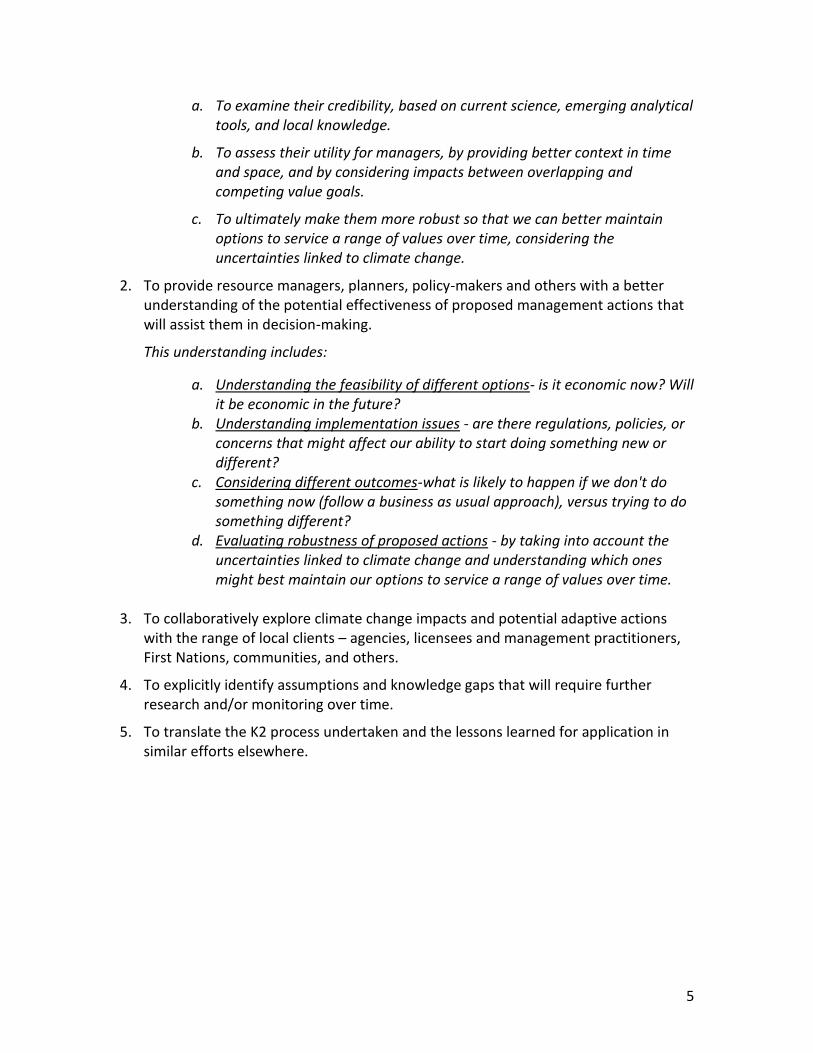
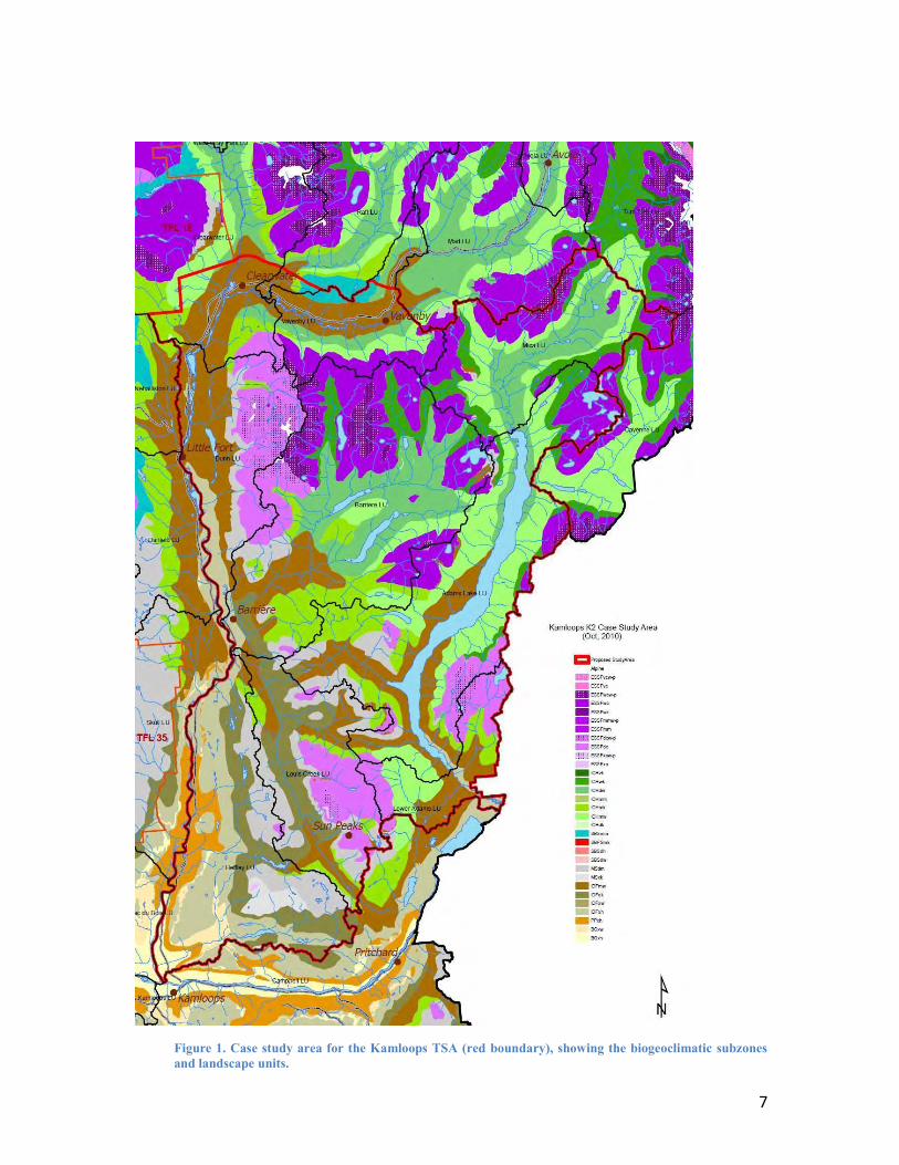
The Kamloops TSA is situated in south-central British Columbia and represents approximately 2.7 million hectares. After exploring the idea of using two case study areas, one at each extreme of the Kamloops TSA, we decided on using one representative study area near the middle of the TSA. A number of criteria entered this decision, including:
the comparative advantages and disadvantages of contiguous or discontinuous stand units,
an appropriate size to accommodate disturbances and biodiversity at the landscape level,
modelling capability and ease, and
the ability to extrapolate results to other areas in the TSA and Southern Interior Forest Region.
The case study area comprises 372,964 ha of productive forest in the Kamloops TSA, mapped with six entire landscape units, and portions of four landscape units, representative of six key groups of 12 biogeoclimatic subzones in the Southern Interior Forest Region:
Ecological Groups (or Ecozones)
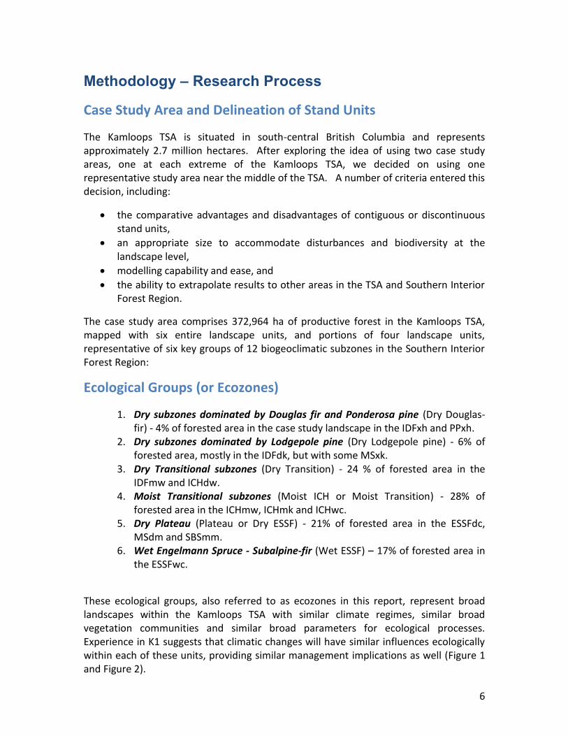
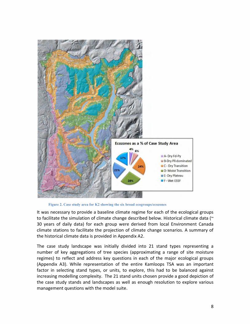
1. Dry subzones dominated by Douglas fir and Ponderosa pine (Dry Douglas-fir) - 4% of forested area in the case study landscape in the IDFxh and PPxh.
2. Dry subzones dominated by Lodgepole pine (Dry Lodgepole pine) - 6% of forested area, mostly in the IDFdk, but with some MSxk.
3. Dry Transitional subzones (Dry Transition) - 24 % of forested area in the IDFmw and ICHdw.
4. Moist Transitional subzones (Moist ICH or Moist Transition) - 28% of forested area in the ICHmw, ICHmk and ICHwc.
5. Dry Plateau (Plateau or Dry ESSF) - 21% of forested area in the ESSFdc, MSdm and SBSmm.
6. Wet Engelmann Spruce - Subalpine-fir (Wet ESSF) – 17% of forested area in the ESSFwc.
These ecological groups, also referred to as ecozones in this report, represent broad landscapes within the Kamloops TSA with similar climate regimes, similar broad vegetation communities and similar broad parameters for ecological processes. Experience in K1 suggests that climatic changes will have similar influences ecologically within each of these units, providing similar management implications as well (Figure 1 and Figure 2).
7
Figure 1. Case study area for the Kamloops TSA (red boundary), showing the biogeoclimatic subzones and landscape units.
8
Figure 2. Case study area for K2 showing the six broad ecogroups/ecozones
It was necessary to provide a baseline climate regime for each of the ecological groups to facilitate the simulation of climate change described below. Historical climate data (~ 30 years of daily data) for each group were derived from local Environment Canada climate stations to facilitate the projection of climate change scenarios. A summary of the historical climate data is provided in Appendix A2.
The case study landscape was initially divided into 21 stand types representing a number of key aggregations of tree species (approximating a range of site moisture regimes) to reflect and address key questions in each of the major ecological groups (Appendix A3). While representation of the entire Kamloops TSA was an important factor in selecting stand types, or units, to explore, this had to be balanced against increasing modelling complexity. The 21 stand units chosen provide a good depiction of the case study stands and landscapes as well as enough resolution to explore various management questions with the model suite.
9
The choice of stand units were ground-truthed to ensure a good representation and linkage to potential modelling questions. The stands associated with the various units range in size, with nine hectares as the smallest size for spatial resolution at the landscape scale.
Note that once the existing GIS data was analysed for our modelling we eliminated one stand unit in the Dry Transition, as there was not enough of it to separate out. As well, because we could not access weather station data for the Wet ESSF ecozone, we would not be able to calibrate climate data for that area and could not model climate change over time. For that reason, our modelling focussed on five ecozones and 19 stand units (Appendix A3).
Overview of the Forest Model Suite
A complete primer on models and modelling can be found in Appendix A1).
K2 utilized five linked forest models to quantify ecological sensitivities and implications from proposed management actions under climate change by exploring a) forest regeneration and growth dynamics and b) alternative management strategies as they unfold across the landscape over time, considering natural disturbance in the face of climate change. The modelling suite includes:
1. TACA – the Tree & Climate Assessment Tool for modelling tree species response to climate change during regeneration.
2. FORWADY - The Forest Water Dynamics Model for simulating forest stand hydrology and its impacts on stand development and regeneration.
3. FORECAST-Climate Model – an updated version of FORECAST to model forest stand growth & ecosystem dynamics with a changing climate (by integrating FORWADY within it).
4. FPS (Forest Planning Studio, formerly known as Atlas) - a spatially explicit forest estate simulation model which allows for incorporation of natural and operational landscape level processes and considerations over time.
5. Dyna-Plan – a spatially explicit simulation and optimization model for projecting forest growth, management activities, and natural disturbances at the landscape level. Here it is being used to simulate natural disturbances together with harvesting over the landscape over time with climate change.
TACA linked with FORWADY addresses the successful establishment and regeneration of various tree species within local ecosystems under a changing climate, while FORECAST addressed ecological dynamics, stand growth and mortality over time. FPS addressed landscape-level structures, ecological dynamics and management activities over time. FORWADY helped TACA determine if regeneration is successful, and subsequently imposes evaporative and transpirational water budgets upon stands within FORECAST. In TACA, environmental conditions were imposed upon a stand of tree species resulting in a cohort of seedlings that “survive” and become established, based on species specific thresholds incorporated into the model. The TACA model provided output regarding
10
establishment probabilities for various tree species that were fed into the FORECAST Climate model for suitable disturbed stand units.
FORECAST Climate used this information to “grow” new stands after a disturbance, as well as moving existing stands along developmental trajectories. Stand growth in the face of climatic stress was calibrated through dendrochronological analyses for a few key species, providing a greater level of confidence. This information was combined with stand-level information describing rates of decomposition, nutrient cycling, and other ecosystem properties to simulate forest growth under a wide range of management and climatic conditions.
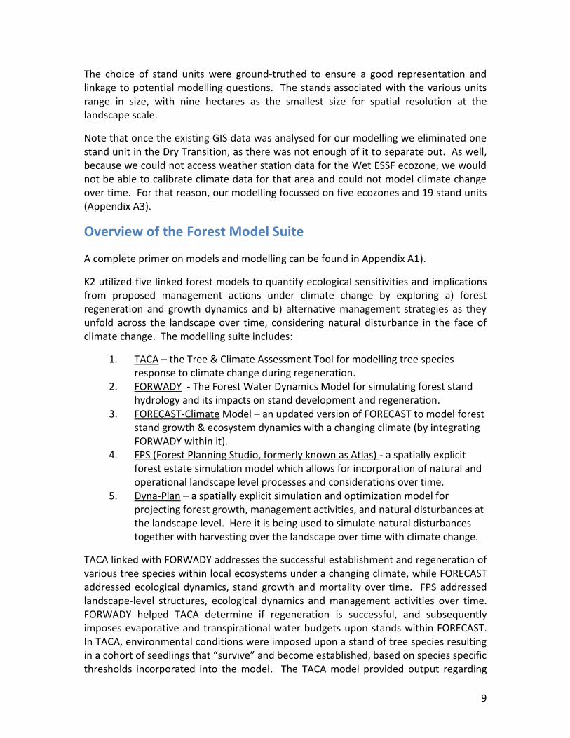
Using FPS, we were able to simulate preferred management strategies for a number of indicators of forest management by accumulating TACA and FORECAST information and providing a spatial landscape context within the case study area, building in landscape processes such as harvesting and natural disturbance (Error! Reference source not found.). Dyna-Plan was also capable of implementing natural disturbances over time as well as seeking optimal harvest schedules from eligible treatment regimes. Each stand, the basic unit used in the model, belongs to an ecosystem group with similar attributes (volumes, snags, coarse woody debris, etc.) for a given age. Once a specific treatment regime is initiated by the model, it implements a set of activities (i.e. clearcut, plant, fertilize) at predetermined times to best meet user defined objectives.
Figure 3. A representation of the linkages between the models (blue diamonds) and their inputs (black boxes), outputs (green), assumptions and scenarios (red boxes). The figure emphasizes inputs and outputs associated with the application FORECAST Climate. The landscape level modelling (FPS) utilized the stand attribute database generated by FORECAST and built in scenarios and assumptions for harvesting and natural disturbance
11
Framing the Modelling - Establishment of Goals, Questions and Indicators
Modelling Goals and Questions
Fundamental to the modelling process is the incorporation of local values, objectives, and indicators, achieved through the involvement of the project clients. To facilitate that process, the K2 team created a “definitions document” to ensure that the understanding of terms used throughout the project was consistent between all team members and clients (Appendix A4). As well, a website2 was created to facilitate sharing of key documents and background information.
K2 clients include forest managers from local resource agencies, and forest companies, as well as local researchers and other knowledgeable stakeholders from the Kamloops TSA area. Through a series of facilitated workshops, the K2 team worked with these folks to identify important management goals and questions, allowing the team to establish a series of indicators and providing context for the modelling process.
2 http://k2kamloopstsa.com
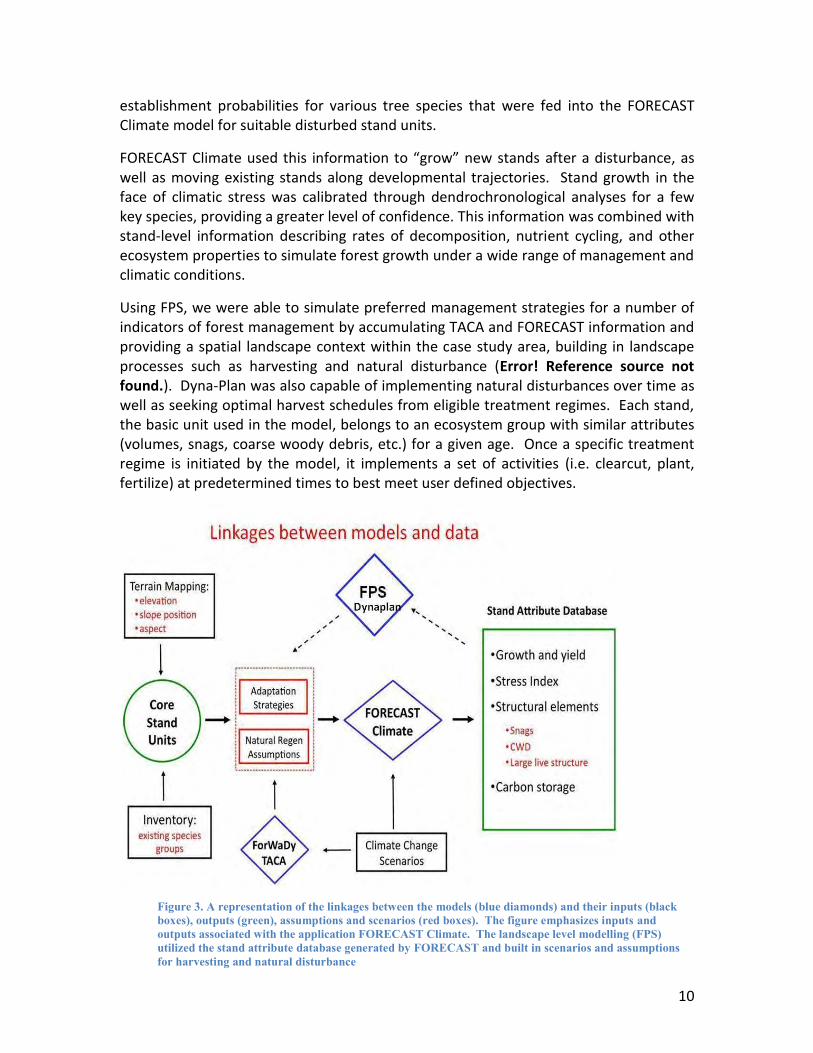
Figure 4. Another visual representation of the modelling framework. This version graphically depicts examples of model inputs (e.g. climate scenarios and adaptation strategies) and projected outputs (e.g. merchantable volume and carbon storage) that were the basis for interpretations.
12
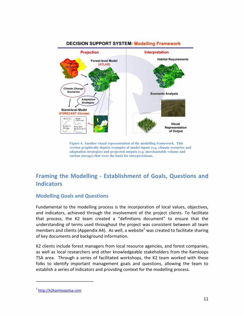
The management goals (not to be confused with the project goals) will be discussed in the conclusions at the end of the report, based on the lessons learned through the modelling and the interpretation and discussion of results (Table 1). They are roughly linked to the intent provided by current 2008 Canadian Standards Association Sustainable Forest Management (CSA SFM) guidance for certification within the TSA. The Timber objective also fits with the stated current provincial direction from the BC Ministry of Forests, Lands and Natural Resource Operations.
Table 1. Local forest management goals to guide modelling and management scenario testing within the K2 project.
Overarching Goal: Encourage resilience within the ecosystems to maintain productive, “healthy” forests that will continue to be able to provide future benefits (for timber, biodiversity, etc.) in spite of the disturbances (and surprises) that may result from climate change.
Timber: Maintain or increase the flow of timber volume and/or value over time.
Habitat & Biodiversity:
No loss of native species due to management over time.
Fire: Minimize fire risk to people and property.
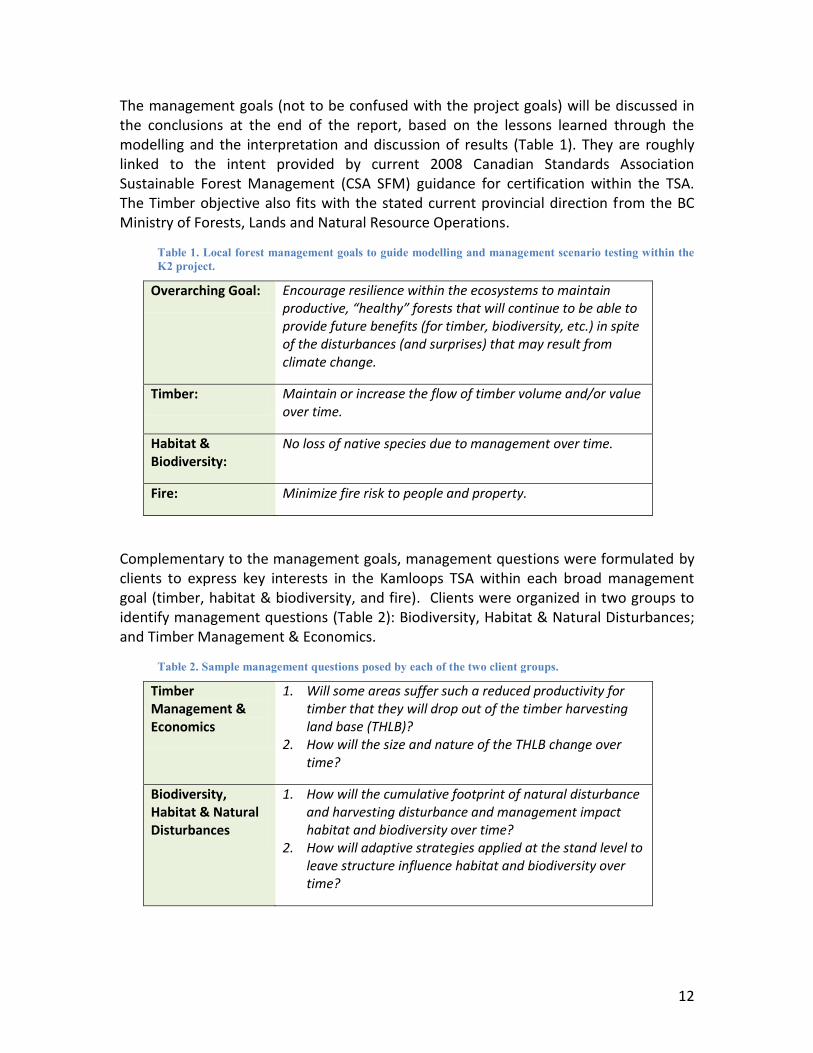
Complementary to the management goals, management questions were formulated by clients to express key interests in the Kamloops TSA within each broad management goal (timber, habitat & biodiversity, and fire). Clients were organized in two groups to identify management questions (Table 2): Biodiversity, Habitat & Natural Disturbances; and Timber Management & Economics.
Table 2. Sample management questions posed by each of the two client groups.
Timber Management & Economics
1. Will some areas suffer such a reduced productivity for timber that they will drop out of the timber harvesting land base (THLB)?
2. How will the size and nature of the THLB change over time?
Biodiversity, Habitat & Natural Disturbances
1. How will the cumulative footprint of natural disturbance and harvesting disturbance and management impact habitat and biodiversity over time?
2. How will adaptive strategies applied at the stand level to leave structure influence habitat and biodiversity over time?
13
The complete list of questions formulated by the working groups (Appendix A5) was used to:
1. Help establish what was possible to address within the scope of the project. 2. Set the priorities to address within the timeframe of the project. 3. Build scenarios and indicators to explore the key priorities. 4. Select and modify inputs to best accommodate the questions and the models. 5. And build and/or modify various aspects of the models to better accommodate
exploration of priority questions.
Modelling Indicators
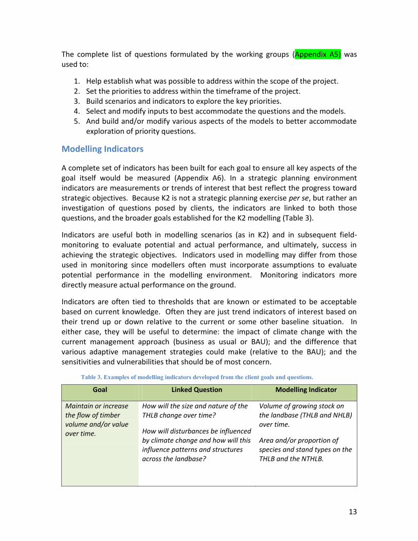
A complete set of indicators has been built for each goal to ensure all key aspects of the goal itself would be measured (Appendix A6). In a strategic planning environment indicators are measurements or trends of interest that best reflect the progress toward strategic objectives. Because K2 is not a strategic planning exercise per se, but rather an investigation of questions posed by clients, the indicators are linked to both those questions, and the broader goals established for the K2 modelling (Table 3).
Indicators are useful both in modelling scenarios (as in K2) and in subsequent field-monitoring to evaluate potential and actual performance, and ultimately, success in achieving the strategic objectives. Indicators used in modelling may differ from those used in monitoring since modellers often must incorporate assumptions to evaluate potential performance in the modelling environment. Monitoring indicators more directly measure actual performance on the ground.
Indicators are often tied to thresholds that are known or estimated to be acceptable based on current knowledge. Often they are just trend indicators of interest based on their trend up or down relative to the current or some other baseline situation. In either case, they will be useful to determine: the impact of climate change with the current management approach (business as usual or BAU); and the difference that various adaptive management strategies could make (relative to the BAU); and the sensitivities and vulnerabilities that should be of most concern.
Table 3. Examples of modelling indicators developed from the client goals and questions.
Goal Linked Question Modelling Indicator
Maintain or increase the flow of timber volume and/or value over time.
How will the size and nature of the THLB change over time?
How will disturbances be influenced by climate change and how will this influence patterns and structures across the landbase?
Volume of growing stock on the landbase (THLB and NHLB) over time.
Area and/or proportion of species and stand types on the THLB and the NTHLB.
14
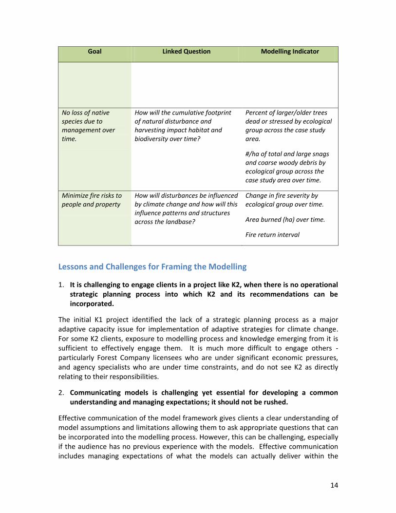
Goal Linked Question Modelling Indicator
No loss of native species due to management over time.
How will the cumulative footprint of natural disturbance and harvesting impact habitat and biodiversity over time?
Percent of larger/older trees dead or stressed by ecological group across the case study area.
#/ha of total and large snags and coarse woody debris by ecological group across the case study area over time.
Minimize fire risks to people and property
How will disturbances be influenced by climate change and how will this influence patterns and structures across the landbase?
Change in fire severity by ecological group over time.
Area burned (ha) over time.
Fire return interval
Lessons and Challenges for Framing the Modelling
1. It is challenging to engage clients in a project like K2, when there is no operational strategic planning process into which K2 and its recommendations can be incorporated.
The initial K1 project identified the lack of a strategic planning process as a major adaptive capacity issue for implementation of adaptive strategies for climate change. For some K2 clients, exposure to modelling process and knowledge emerging from it is sufficient to effectively engage them. It is much more difficult to engage others - particularly Forest Company licensees who are under significant economic pressures, and agency specialists who are under time constraints, and do not see K2 as directly relating to their responsibilities.
2. Communicating models is challenging yet essential for developing a common understanding and managing expectations; it should not be rushed.
Effective communication of the model framework gives clients a clear understanding of model assumptions and limitations allowing them to ask appropriate questions that can be incorporated into the modelling process. However, this can be challenging, especially if the audience has no previous experience with the models. Effective communication includes managing expectations of what the models can actually deliver within the
15
scope of the project and conveying the computational complexity of exploring every interesting scenario that could possibly be explored.
3. The best modelling indicators require some context.
The most useful modelling indicators require some context based on a thorough exploration of potential future forest issues, and subsequent management goals and questions that are of most interest to the clients. The time spent within the project to address this challenge was worthwhile as it permitted development of a suite of indicators that are both meaningful to the clients and relevant for the modelling process. Fundamental, however, is a shared understanding amongst clients and researchers of the models, their assumptions and limitations.
Modelling Approach
Design of Management Scenarios to Explore Management Questions
In communicating model assumptions and exploring management questions with clients and in team meetings, it became clear that there were an enormous number of potential scenarios that could be explored with modelling. There was the potential for a number of potential climate change futures to be explored and considered at different time periods with current approaches to forest management as well as various management adaptations with five different linked ecological models. It became obvious that all these options would quickly lead to an unworkable potential number of modelling runs.
In an effort to address this concern, the K2 team used management goals, management questions, and a thorough discussion of indicators to focus in on the most useful and feasible set of scenarios to be explored with the suite of models. The following are the two themes that the K2 project used with two different climate futures (a no climate change and high climate change scenario) over several key points in the future:
1. Business as Usual (BAU) theme - reflects harvesting and silviculture planning and decisions as currently carried out across the case study area. A detailed description of this theme is described in Appendix A7.
2. Alternate Regeneration management theme – diversifying stand types across the landscape through reforestation with tree species less sensitive to climate change, as a strategy to increase resilience.
The Business as Usual (BAU) scenario is intended to explore current management approaches with climate change (BAUCC or BAU with HCC3) and without a changing
3 HCC – High climate change scenario (see the climate data we used linked to specific climate change
scenarios)
16
climate (BAU base case or BAU with NCC4). The purpose of this exercise is to ascertain the potential impacts of climate change on current management approaches and regimes using selected indicators to reflect the impacts on various management goals (timber, habitat, fire). It also facilitates an assessment of the robustness of the initial ecological and management impacts assumptions developed during K1 to explore management actions under climate change.5
The BAU with HCC scenario was used as a comparison (using the climate change data set) against the alternative regeneration adaptation scenario designed using the modelling questions and recommendations from K1. Comparisons indicate the extent of improvement provided by the adaptation measure, and comparison with the BAU with NCC indicates how the scenario compares to our future determined with our current management without climate change. This is critical to understanding the cumulative difference that adaptive actions may or may not make to increase resilience.
Acquiring Climate Data
Climate Change Futures (Scenarios) and Data
To incorporate projections of climate change, K2 used projected relative mean monthly precipitation and temperature data from general circulation models (GCM) with climate-forcing assumptions from a High carbon emissions scenario6. This provided a climate scenario that was examined for the years 2020, 2050, and 2080 across the case study landscape. Having a High climate change scenario is useful because it represents an extreme for a range of plausible impacts from which forest and range management can be evaluated.
A short list of GCMs were recommended by both the Pacific Climate Impacts Consortium (PCIC) and the BC Ministry of Forests, Mines, and Lands for their robustness in the province7. From the recommended list and available SRES8 global emissions scenarios, the following GCM/emission combination was selected:
1. High change future (scenario) = A1B carbon emission scenario, using three GCMs: a. UKMO_HADGEM1 b. MIROC32_HIRES c. UKMO_HADCM3
4NCC – No climate change
5 More information about K1 can be found at http://k2kamloopstsa.com/backgrounder-2/
6 HIGH emissions scenario – An IPCC global carbon emissions scenario assuming global conditions of rapid
economic growth with a balanced emphasis on all energy sources, including fossil fuels. Note that this is not the most pessimistic emissions scenario. The A1FI assumes rapid growth with a reliance on and expanding use of fossil fuel energy.
7 Bonsal, B.R., Prowse T.D., Piertroniro, A. 2003. An assessment of global climate model-simulated climate
for the western cordillera of Canada (1961-90). Hydrological Processes. 17, 3703-3716. 8 Intergovernmental Panel on Climate Change Special Report on Emissions Scenarios (SRES):
http://www.grida.no/publications/other/ipcc_sr/?src=/climate/ipcc/emission/
17
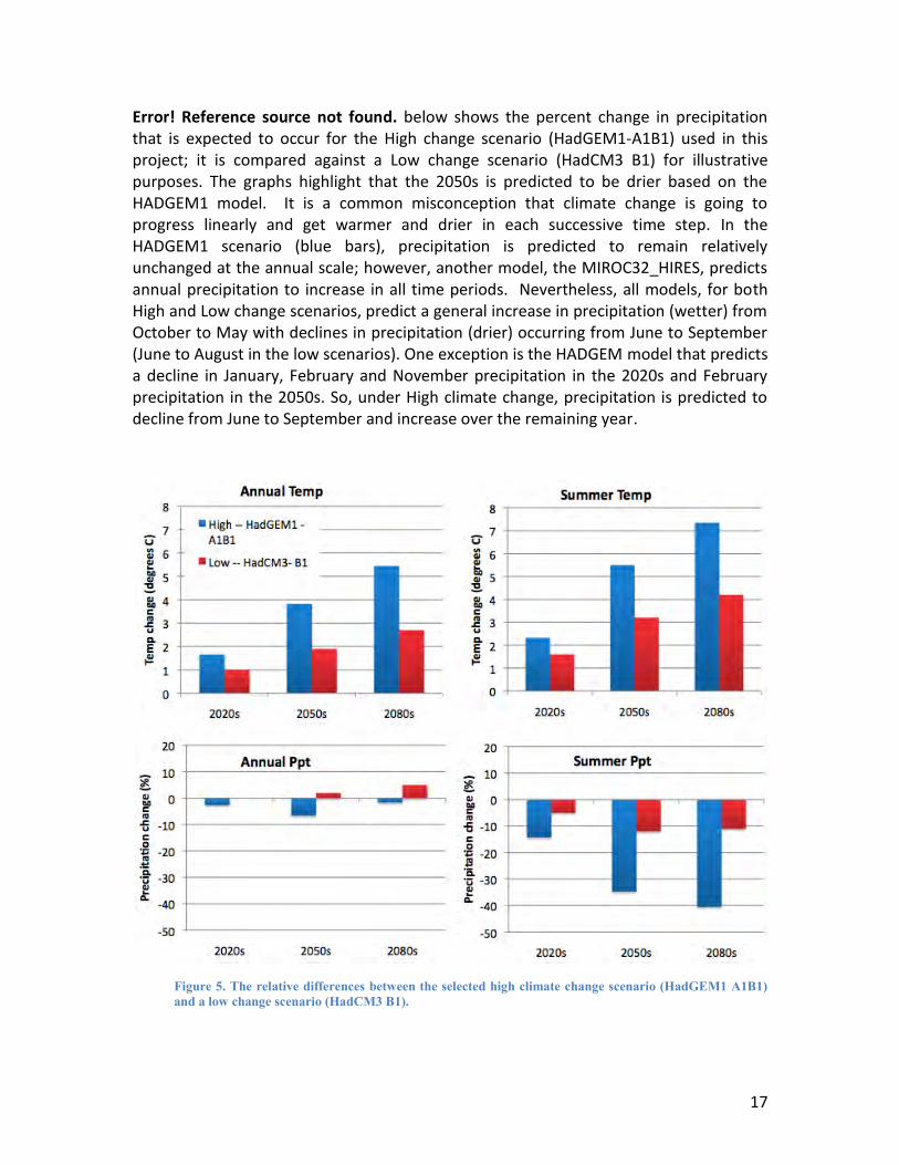
Error! Reference source not found. below shows the percent change in precipitation that is expected to occur for the High change scenario (HadGEM1-A1B1) used in this project; it is compared against a Low change scenario (HadCM3 B1) for illustrative purposes. The graphs highlight that the 2050s is predicted to be drier based on the HADGEM1 model. It is a common misconception that climate change is going to progress linearly and get warmer and drier in each successive time step. In the HADGEM1 scenario (blue bars), precipitation is predicted to remain relatively unchanged at the annual scale; however, another model, the MIROC32_HIRES, predicts annual precipitation to increase in all time periods. Nevertheless, all models, for both High and Low change scenarios, predict a general increase in precipitation (wetter) from October to May with declines in precipitation (drier) occurring from June to September (June to August in the low scenarios). One exception is the HADGEM model that predicts a decline in January, February and November precipitation in the 2020s and February precipitation in the 2050s. So, under High climate change, precipitation is predicted to decline from June to September and increase over the remaining year.
Figure 5. The relative differences between the selected high climate change scenario (HadGEM1 A1B1) and a low change scenario (HadCM3 B1).
18
Based on an ensemble of the scenarios (as used in the modeling), precipitation is expected to be higher in the 2080s vs. 2050s. The decline in summer precipitation is larger in the 2080s than the 2050s but the increase in autumn, spring and winter precipitation is far greater. Thus in the 2080s, non-summer precipitation is offsetting the decline in summer precipitation at the annual scale but in the 2050s this is not occurring to the same extent leading to a larger annual decline in precipitation.
The climate scenarios utilized in K2 are slightly different from those used in the K1 project for several reasons. First, they have been updated since K1, in the latest IPCC Fourth Assessment Report and therefore are assumed to reflect the current science being used to describe potential climate change. Secondly they were recommended to the K2 team by FFESC advisors from the Pacific Climate Impacts Consortium (PCIC). The projected relative mean monthly climate data was applied to a relative time sequence in order to simulate a period of continual climate change, which was then used in the K2 modelling. This was done in the following manner:
The time period from 2010 to 2035 uses the 2020 projected climate data.
The 2036 - 2065 period uses the 2050 projected climate data.
The 2066 - 2100 period uses the 2080 projected climate data.
Downscaling and Projecting Annual Variability using Daily Time-steps
Projected relative mean monthly precipitation and temperature data for the climate scenario were downscaled to the case study area using daily data from local climate stations to reflect local variation in elevation, latitude and aspect across the K2 area. Thirty years of daily climate data (1975-2004) were used as the basis for the historical and climate change simulation scenarios. A summary of the climate data used to represent each of the ecogroups is provided in Appendix A2.
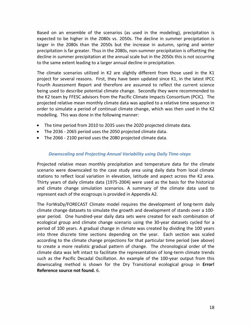
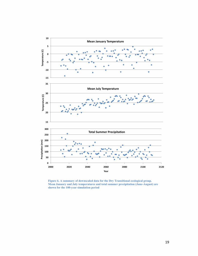
The ForWaDy/FORECAST Climate model requires the development of long-term daily climate change datasets to simulate the growth and development of stands over a 100-year period. One hundred-year daily data sets were created for each combination of ecological group and climate change scenario using the 30-year datasets cycled for a period of 100 years. A gradual change in climate was created by dividing the 100 years into three discrete time sections depending on the year. Each section was scaled according to the climate change projections for that particular time period (see above) to create a more realistic gradual pattern of change. The chronological order of the climate data was left intact to facilitate the representation of long-term climate trends such as the Pacific Decadal Oscillation. An example of the 100-year output from this downscaling method is shown for the Dry Transitional ecological group in Error! Reference source not found. 6.
19
Figure 6. A summary of downscaled data for the Dry Transitional ecological group. Mean January and July temperatures and total summer precipitation (June-August) are shown for the 100-year simulation period
20
Designing Modeling Scenarios - Combining Climate Futures with Management Scenarios
When the two climate futures options are combined with the management scenarios the number of potential modeling scenarios expands. To allow for flexibility particularly with the landscape modeling, the following modeling scenarios were designed to be worked through sequentially:
Modelling Scenarios
1. Business-as-usual (BAU) with no climate change (No CC) 2. BAU with HIGH CC HCC) 3. Alternative regeneration species with HIGH CC (Alt Regen CC)
The BAU no CC and BAU HCC scenarios were developed to address the current approach to management and provide a baseline from which to measure the effects of climate change on current management systems. The business-as-usual (BAU) scenario was defined using many of the same assumptions and inputs for the latest timber supply review (TSR) in the Kamloops TSA for appropriate stands. In some cases other data sources were utilized to help clarify the BAU scenarios. For example, the provincial silviculture history database (RESULTS) was consulted to determine current tree species planting preferences in the K2 stand units based on practices over the past decade.
A third scenario, Alternative regeneration species with HIGH CC, was developed to evaluate the efficacy of potential adaptation strategies associated with planting of different species that may be better suited to the high climate change regime. It was of interest to the K2 clients, reflected by their modeling questions. Alternative regeneration species were determined for selected stand units based upon output from the TACA model. In this scenario, the selected alternative species were planted following harvesting rather than the species used in the BAU scenario.
Lessons and Challenges for Designing Scenarios
1. It is critical to anticipate the range of potential modelling runs in advance to set limits and priorities.
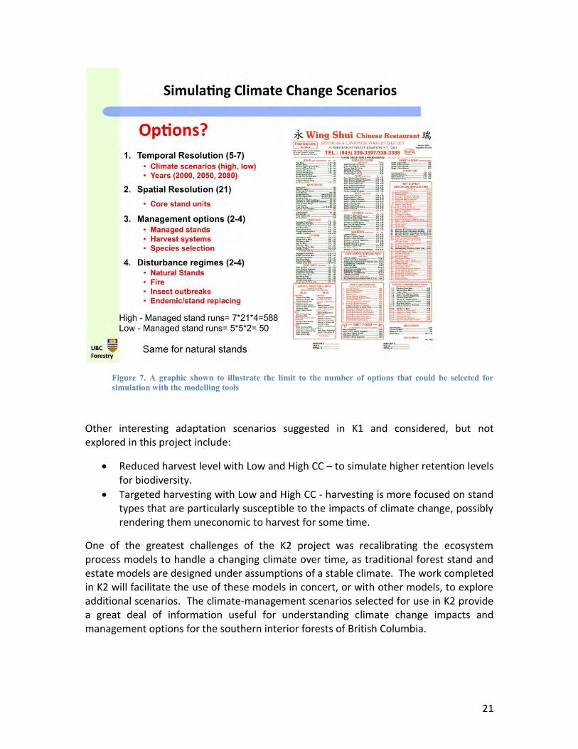
The number of potential modelling runs can become unworkable, when scenario options for climate change are combined with temporal reporting options (2050, 2080 etc) and options for management and/or modelling assumptions. It is important to narrow down the priorities for potential runs to focus the time and effort. This links back with a previous lesson that it is important to communicate the modelling framework effectively to manage expectations. It was useful for this project to develop a “menu,” so to speak, of management/climate scenarios from which the clients could select what they were most interested in examining. The slide shown in Figure 7 was presented during a client workshop in Kamloops (February 10, 2010) to illustrate the fact that options for the modelling scenarios were limited by what was practical.
21
Figure 7. A graphic shown to illustrate the limit to the number of options that could be selected for simulation with the modelling tools
Other interesting adaptation scenarios suggested in K1 and considered, but not explored in this project include:
Reduced harvest level with Low and High CC – to simulate higher retention levels for biodiversity.
Targeted harvesting with Low and High CC - harvesting is more focused on stand types that are particularly susceptible to the impacts of climate change, possibly rendering them uneconomic to harvest for some time.
One of the greatest challenges of the K2 project was recalibrating the ecosystem process models to handle a changing climate over time, as traditional forest stand and estate models are designed under assumptions of a stable climate. The work completed in K2 will facilitate the use of these models in concert, or with other models, to explore additional scenarios. The climate-management scenarios selected for use in K2 provide a great deal of information useful for understanding climate change impacts and management options for the southern interior forests of British Columbia.
22
Impacts of Climate Change on Regeneration Success: Species Level Modelling with TACA
Model Description
The ecological model, TACA (Tree And Climate Assessment) (Nitschke and Innes 2008), was parameterised for use in the ecosystems of the K2 study area. TACA is a mechanistic species distribution model (MSDM) that analyzes the response of trees to climate. It assesses a species’ probability to regenerate, grow and survive under a range of climatic and soil conditions. The modelling approach reflects both the regeneration potential of a species, since presence is directly related to establishment (McKenzie et al. 2003), and the climatic suitability of an area for a given species.
The TACA model takes into consideration many of the phenological relationships known as requirements or limiting factors for the successful establishment of a given species under specific climate and soil conditions. The results from TACA often require careful interpretation, as there can be complex interactions among the phenological variables considered which may sometimes generate counterintuitive results. A detailed description of TACA and its application are provided in Appendix 8. A summary of its application is provided below.
Model Application
An analysis of the effect of climate change on the expected regeneration patterns of 16 different species within the Kamloops study area was completed using the TACA model in combination with the climate change data described above. TACA requires a measure of variability of the historical climate data to simulate the range of climate years that may occur in the future. Based on a rank and percentile test, 10 historical years of climate data were selected for each station and used as the historical climate scenarios in the analysis. The 10 years of data represent the 90th, 75th, 50th, 25th, and 10th percentiles for both observed annual precipitation and mean annual temperature.
Duplicity between temperature and precipitation scenario selection was resolved using an annual heat-moisture index metric [(Mean Annual Temperature + 10)/ (Precipitation/1000)] (Wang et al., 2006) to select additional years from the climate distribution not covered by the initial selection criteria. The selected historical climate scenarios were used as the foundation for developing different climate change scenarios that incorporate daily climate variation. Bürger (1996) stated that incorporating daily climatic variation is important for improving the realism of climate change scenarios. The incorporation of extreme climate years is also important as species distributions are influenced by climatic extremes (Zimmerman et al., 2009).
The selected ten years of daily data were subsequently downscaled using a direct approach to reflect the expected climate change patterns as derived from the GCM models/scenarios.
23
The analysis was structured such that the probability of successful establishment was calculated for each species, climate change scenario and ecological group combination. The analysis was further stratified to consider the relative impact of soil edaphic conditions on establishment success. A table was created for each species to summarize model output.
Linking TACA Output with FORECAST Climate
Output from the regeneration analysis conducted with TACA was used to determine the regeneration patterns to be simulated with FORECAST Climate for the different stand units under the high climate change scenarios. Regeneration patterns in the BAU No CC scenario were assumed to remain constant in the future. This process was conducted by starting with the species and densities that would be expected to occur in the natural and managed stand units and adjusting the expected number of established trees depending on the probability of establishment projected by TACA with climate change. Specifically, the model provided output for the probability of regeneration success for each species and stand unit combination, taking into account edaphic class (submesic, mesic, or subhygric), the climate regime associated with each ecogroup, and the regeneration period (P1 = 2010-2035, P2 = 2036-2065, P3 = 2066-2110). The specific regeneration assumptions used for each stand unit and regeneration period combination are shown for natural and managed stand units in Appendix 9.
Modelling Impacts of Climate Change on Future Growth: Stand Level Modelling with FORECAST Climate
Model Description
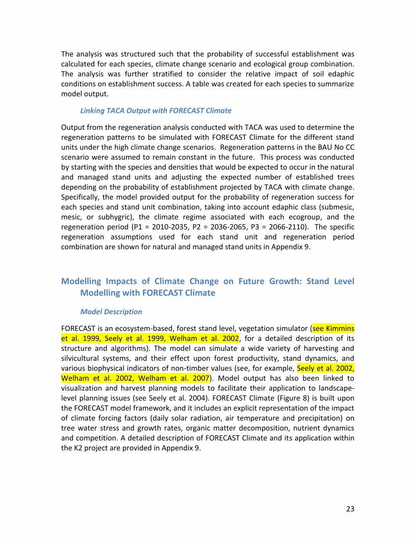
FORECAST is an ecosystem-based, forest stand level, vegetation simulator (see Kimmins et al. 1999, Seely et al. 1999, Welham et al. 2002, for a detailed description of its structure and algorithms). The model can simulate a wide variety of harvesting and silvicultural systems, and their effect upon forest productivity, stand dynamics, and various biophysical indicators of non-timber values (see, for example, Seely et al. 2002, Welham et al. 2002, Welham et al. 2007). Model output has also been linked to visualization and harvest planning models to facilitate their application to landscape-level planning issues (see Seely et al. 2004). FORECAST Climate (Figure 8) is built upon the FORECAST model framework, and it includes an explicit representation of the impact of climate forcing factors (daily solar radiation, air temperature and precipitation) on tree water stress and growth rates, organic matter decomposition, nutrient dynamics and competition. A detailed description of FORECAST Climate and its application within the K2 project are provided in Appendix 9.
24
Figure 8. A schematic showing the basic ecosystem components represented within FORECAST Climate
Forecast Climate Evaluation with Dendrochronology
A dendroclimatology field study was undertaken during the summer of 2010 to evaluate the effect of past climate regimes on tree growth within the Kamloops study area. The study was focussed on the growth of developing lodgepole pine and Douglas-fir stands within two general site types: 1) Dry IDF dk and 2) Moist ICH mw/mk. Stem analysis cookies were taken from a total of 240 trees (120 Pl and 120 Fd) during July 2010. The cookies have been processed and measured in the Tree Ring Lab at the University of Northern British Columbia (overseen by Kathy Lewis). Data from the analysis was used to evaluate the capability of FORECAST Climate to project patterns of climate growth response for Douglas-fir and lodgepole pine.
FORECAST Climate Simulations
FORECAST Climate was run to simulate all the different stand units described in Appendix 3. Initially, all of the core stand units (Appendix 3) were split into managed or natural stand types and simulated using cycled (30-year) historic daily climate data for time periods of up to 300 years (depending on the stand type). The climate change simulations required many more analysis units to accommodate the complexity associated with simulating the onset of climate change.
Potential Net PrimaryPotential Net Primary
ProductionProduction
(Potential growth)(Potential growth)
Actual Net PrimaryActual Net Primary
ProductionProduction
(Actual growth)(Actual growth)
LitterLitterCoarse woodyCoarse woodydebrisdebrisFine rootsFine roots
Nutrient poolNutrient pool
Nutrient cyclingNutrient cycling
Climate
Wateravailability
Transpira on
Ou low
Waterstress
25
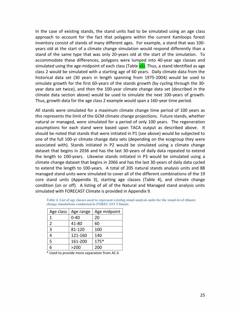
In the case of existing stands, the stand units had to be simulated using an age class approach to account for the fact that polygons within the current Kamloops forest inventory consist of stands of many different ages. For example, a stand that was 100-years old at the start of a climate change simulation would respond differently than a stand of the same type that was only 20-years old at the start of the simulation. To accommodate these differences, polygons were lumped into 40-year age classes and simulated using the age-midpoint of each class (Table x5). Thus, a stand identified as age class 2 would be simulated with a starting age of 60 years. Daily climate data from the historical data set (30 years in length spanning from 1975-2004) would be used to simulate growth for the first 60-years of the stands growth (by cycling through the 30-year data set twice), and then the 100-year climate change data set (described in the climate data section above) would be used to simulate the next 100-years of growth. Thus, growth data for the age class 2 example would span a 160-year time period.
All stands were simulated for a maximum climate change time period of 100 years as this represents the limit of the GCM climate change projections. Future stands, whether natural or managed, were simulated for a period of only 100 years. The regeneration assumptions for each stand were based upon TACA output as described above. It should be noted that stands that were initiated in P1 (see above) would be subjected to one of the full 100-yr climate change data sets (depending on the ecogroup they were associated with). Stands initiated in P2 would be simulated using a climate change dataset that begins in 2036 and has the last 30-years of daily data repeated to extend the length to 100-years. Likewise stands initiated in P3 would be simulated using a climate change dataset that begins in 2066 and has the last 30-years of daily data cycled to extend the length to 100-years. A total of 205 natural stands analysis units and 88 managed stand units were simulated to cover all of the different combinations of the 19 core stand units (Appendix 3), starting age classes (Table 4), and climate change condition (on or off). A listing of all of the Natural and Managed stand analysis units simulated with FORECAST Climate is provided in Appendix 9.
Table 4. List of age classes used to represent existing stand analysis units for the stand-level climate change simulations conducted in FORECAST Climate.
Age class Age range Age midpoint
1 0-40 20
2 41-80 60
3 81-120 100
4 121-160 140
5 161-200 175*
6 >200 200 * Used to provide more separation from AC 6
26
FORECAST Climate Output
FORECAST Climate produces a diverse set of output. Output was summarized for each of the 293 analysis units (Appendix X2a and X2b) including merchantable volume by species, snags all sizes, snags (>30cm dbh), logs all sizes, logs (>30cm diameter), top height, stand density, and annual water stress index. These data were used to construct a stand attribute database that was subsequently linked to the landscape-scale models FPS and Dyna-Plan to facilitate landscape-scale analyses of attributes and indicators.
Landscape Level Modelling with FPS and Dyna-Plan
Landscape Model Choice
There is a wide variety of landscape scale models used in forest management planning, each with associated strengths and weaknesses. Two different but complementary landscape-scale models were selected to accommodate the diverse simulation needs of this project: 1) FPS-ATLAS and 2) Dyna-Plan. Each model is described in general terms in the following section and each is described in detail in associated appendices.
FPS-ATLAS (henceforth referred to as FPS) is a spatially explicit forest estate simulation model that allows for incorporation of natural and operational landscape level processes and considerations over time.9 It has been widely used throughout BC and was selected to provide an analysis of climate change impacts within a forest planning framework that is familiar to Kamloops forest managers, as it reflects the approach used in BC timber supply reviews (TSR). Further, its linkage to FORECAST is well documented (see, for example (Seely, et al., 2004). More detail on FPS and its application in the K2 Project can be found in Appendix A10.
The other landscape-scale model selected for the landscape-scale simulation of climate change impacts is the Dyna-Plan model. Dyna-Plan differs from FPS in that Dyna-Plan was constructed on raster-based GIS platform and employs a cellular automaton approach that allows it calculate optimal solutions to achieve spatially specific forest management goals. Further, the flexible structure within Dyna-Plan allows it to more easily represent spatial dynamics of natural disturbance agents such as fire while including algorithms for fire spread and fire size distributions. In K2, Dyna-Plan has been used to simulate natural disturbances together with harvesting over the landscape over time with climate change. More detail on Dyna-Plan can be found in Appendix A11.
9 For more information, see www.forestry.ubc.ca/atlas-simfor/project/about.html
27
Application of Landscape-scale Models
A large amount of input and calibration information is required to complete landscape projections and harvest estimates. This information was obtained in four broad categories: land base, forest inventory, management practices, and forest dynamics. This information was then translated into a model formulation that explored sustainable rates of harvest in the context of integrated resource management and natural disturbance with and without climate change.
Integration with FORECAST, TACA, the Climate Data Set and Management Scenarios
Modelling progressive climate change at the landscape level with daily time steps is extremely challenging and is beyond the scope of this project. However, it is possible to model progressive climate change using a relatively simple approach.
To accomplish progressive climate changes, the landscape models were applied with a focus on the differences between: the current climatic situation; the climate projected in 2050; and the climate projected in 2080. The impacts associated with climate change are represented through 2 broad mechanisms:
1. Changing data curves for timber yield and other attributes within each stand unit.
Data curves for each stand unit (designed in FORECAST) change with climate over the three broad time periods described above. These curves reflect the following impacts from climate change: (a) changes in growth (productivity); (b) changes in mortality from insects and disease; (c) changes in mortality directly from increased climatic stress.
2. Altered natural disturbance regimes (wildfire).
Landscape-level natural disturbances are expected to be significantly modified by climate change. Impacts from insect and disease were partially addressed at the stand unit level with FORECAST. Landscape level fire disturbances with fire risks responding to changing climatic factors, was simulated differently with FPS and DYNA-PLAN. These different approaches were chosen to fit with the general modelling approach used by the different models and to provide the K2 team with two different approaches to compare.
The FPS-ATLAS modelling employed a commonly used approach in timber supply analyses to represent the impact of natural disturbance agents on volume flow in the timber harvesting landbase (THLB) and on age class distributions in the non-timber harvesting landbase (NHLB). In FPS most of the mortality from natural disturbance events was assumed to be captured through salvage harvesting, however, it was recognized that a proportion of live stands killed through fire events would not be salvaged. To account for losses from such fire events in the THLB, the model ‘harvested’ an extra volume of timber in each time period that is not included in the reported harvest levels and was assumed to represent unsalvaged or non-recoverable losses (NRLs). The locations and spatial implementation of these NRL fire events were
28
randomly selected and hardwired into the model prior to the model run starting. No attempt was made to model fire size distributions or fire shapes.
With Dyna-Plan, we used a more sophisticated approach to simulate the spread of fire based upon fuel types using a stochastic simulation with targets for total area burned and fire size distributions. Fuel types and loads affect fire spread, but the model burns the predetermined amount of land by placing fires on the land until the fires burn enough land per time step.
In both cases, the amount of area burned within specific ecogroups was increased proportionally by adjusting fire return intervals from the Biodiversity Guidebook to account for the climate change scenarios used in the K2 project (Nitschke and Innes 2007, 2008b). This approach links a warmer drier climate to drier forest fuel conditions, which in turn increases: the chance of successful fire ignition and propagation, the risk of extreme fire behaviour, and the length of the fire season. A trend curve for each ecozone showed a proportional increase over time in the projected area burned in each modelling period. These data were similarly used as an input in both models.
The differences reported for area burned over time between the two models was a result of the different approaches used to calculate the baseline annual area burned prior to using the Nitschke-Inness adjustment factors calculated for the K2 climate scenarios. The approach used in FPS employed a correction factor that changed the Biodiversity Guidebook baseline for the fire return interval (no climate change) for each ecogroup, while the approach used in Dyna-Plan uses the Biodiversity Guidebook value directly. The end result is that baseline annual area burned in the Dyna-Plan approach is approximately 2 times higher than that in FPS ATLAS.
While the two approaches could be considered to represent ‘bookends’ on the actual fire regimes that may occur under climate change, we feel the more sophisticated approach employed with the Dyna-Plan modelling may be more realistic and certainly more conservative from a timber availability perspective than the approach used with FPS. Detailed rationale for our preference for Dyna-Plan’s approach for fire and descriptions of the methods employed to simulate fire in each of the landscape models are provided in Appendix A12.
Modelling Challenges
1. Modelling adaptive scenarios for climate change at the landscape level is complex. Assumptions that are needed to expedite the process must be transparent.
While it is always desirable to try simulations in a realistic fashion that remains true to ecological processes and likely human choices, often some assumptions must be made to simplify the modelling and stay within timeframes and budgets. It is critical that these assumptions are clear so that results can be interpreted within the appropriate context.
29
2. Modelling a business-as-usual rate of harvest is challenging on a subunit within a management unit using climate change data that only spans 100 years.
The landscape modelling (FPS and Dyna-Plan) used typical harvesting criteria found in timber supply review (TSR) analyses, such as harvesting with the “relative-oldest-first” rule using a minimum volume of 100 m3/ha and a minimum of 90% of the culmination of mean annual increment. Landscape level constraints typically included in TSR, such as netdowns for identified species habitat and OGMA’s were included in the modelling. The non-timber harvesting landbase was delineated based on provincial GIS data.
However, both models were challenged to model rate of harvest under a business-as-usual approach on the case study area, when annual allowable cut (AAC) levels are determined at a much coarser scale over the entire TSA. As well, the typical timber supply review process (TSR) used to help determine AACs projects landscape level modelling over 250+ years to establish sustainable harvest flows. Because K2 only developed yield tables influenced by climate change for 100 years, landscape modelling only considered the next 100 years to establish a sustainable harvest flow. Consequently rate of harvest was set for both models to maximize timber flows within the bounds of landscape level constraints over the 100 year period. Actual harvest levels were different between FPS and Dyna-Plan (see Research Outcomes) due to differences in modelling approaches for natural disturbance and the way actual harvest decisions are made in the two models (not the assumptions).
Accordingly, interpretations of the impact of climate change on sustainable harvesting rates must consider the implications for timber supply beyond the 100 year modelling period based on resulting levels of growing stock and age class distributions across the Case Study Area at the end of the 100 year timeframe.
3. Modelling adaptive regeneration strategies is challenging using climate change data that only spans 100 years.
Under the alternate regeneration strategy scenario, species mixes for regeneration were chosen in FORECAST Climate that were thought to be better adapted for climate change over time. When the resulting attribute data curves were used as input for the landscape models, some anticipated results were difficult to evaluate within a 100 year timeframe. Examples of these results include: reduced mortality, improved growing stock, and possibly better timber supply.
The alternate regeneration strategies may take 30-50 years to accumulate enough area across the case study unit to make a significant difference to these landscape level indicators. As well, each stand to which these alternate strategies will apply, requires 40- 50 years plus to accumulate enough volume to make a significant contribution to these indicators. Therefore, it is difficult to influence these indicators in a significant way within a 100 year timeframe.
30
Research Outcomes
Species Level Results (TACA Results)
Using historical and modelled climate data, TACA modelled species, subzone, and site series combinations within the study area to provide regeneration probabilities that were used to inform FORECAST model runs.
Summary of Results
The probability of regeneration success showed a gradual shift towards ponderosa pine and Douglas-fir at lower elevations with increases in their regeneration suitability at higher elevations. Interior spruce, Engelmann spruce, subalpine fir and lodgepole pine had reduced establishment probabilities (i.e. a reduction in their regeneration suitability) which resulted in a gradual decline in the proportion of these species within future stand units in the modelling. Lodgepole pine was particularly affected at lower elevation stand units but may increase at higher elevations by the 2080s. Douglas-fir showed reduced establishment probability in the warmest and driest stand units while ponderosa pine showed an increase in proportion within these drier and warmer stand units. Note however that TACA output is based on climate stations in the open. Douglas-fir in the hot dry subzones requires shade for regeneration success, thus the TACA output on Douglas-fir for these hot dry ecosystems is over-estimated by TACA. However a sensitivity analysis was done to investigate regeneration in an understory (see below).
TACA shows an increase in limiting factors as climate change progresses in the case study area; this is evident in the second and third climate periods modelled (2050s and 2080s, respectively), where regeneration success is reduced for various species in various ecological groups. By the third climate period (2080s) none of the species are regenerating as well as they are currently. As a sensitivity analysis, TACA was used to model regeneration probability for stands with an overstory. The results indicated that for most species, response to climate change was mediated by understory microclimatic conditions allowing many species to continue to regenerate within the shelter of established stands.
At higher elevations, species from lower elevations may be able to regenerate with greater success within the canopies of existing stands as the risk of growing season frost damage is reduced while plenty of precipitation continues to be provided; western red cedar and Douglas-fir are species that may benefit from these conditions. Interior spruce, Douglas-fir and western red cedar will also benefit at lower elevations through a reduction in potential drought stress provided in these sheltered microclimatic conditions. For this project the TACA output from the overstory sensitivities were not included in the stand level modelling due to a concern of a significant increase in output stand level analysis units beyond that which the project could reasonably handle.
31
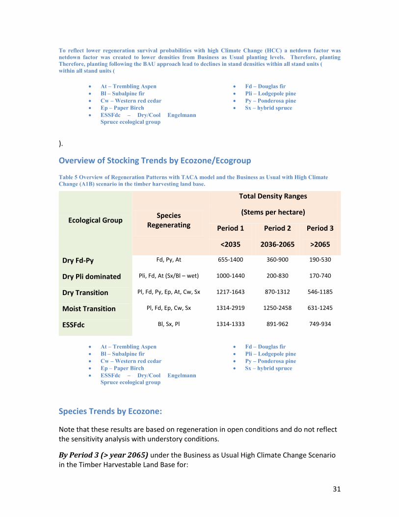
To reflect lower regeneration survival probabilities with high Climate Change (HCC) a netdown factor was netdown factor was created to lower densities from Business as Usual planting levels. Therefore, planting Therefore, planting following the BAU approach lead to declines in stand densities within all stand units ( within all stand units (
At – Trembling Aspen Bl – Subalpine fir Cw – Western red cedar Ep – Paper Birch ESSFdc – Dry/Cool Engelmann
Spruce ecological group
Fd – Douglas fir Pli – Lodgepole pine Py – Ponderosa pine Sx – hybrid spruce
).
Overview of Stocking Trends by Ecozone/Ecogroup
Table 5 Overview of Regeneration Patterns with TACA model and the Business as Usual with High Climate Change (A1B) scenario in the timber harvesting land base.
Ecological Group Species
Regenerating
Total Density Ranges
(Stems per hectare)
Period 1
<2035
Period 2
2036-2065
Period 3
>2065
Dry Fd-Py Fd, Py, At 655-1400 360-900 190-530
Dry Pli dominated Pli, Fd, At (Sx/Bl – wet)
1000-1440 200-830 170-740
Dry Transition Pl, Fd, Py, Ep, At, Cw, Sx
1217-1643 870-1312 546-1185
Moist Transition Pl, Fd, Ep, Cw, Sx
1314-2919 1250-2458 631-1245
ESSFdc Bl, Sx, Pl
1314-1333 891-962 749-934
At – Trembling Aspen Bl – Subalpine fir Cw – Western red cedar Ep – Paper Birch ESSFdc – Dry/Cool Engelmann
Spruce ecological group
Fd – Douglas fir Pli – Lodgepole pine Py – Ponderosa pine Sx – hybrid spruce
Species Trends by Ecozone:
Note that these results are based on regeneration in open conditions and do not reflect the sensitivity analysis with understory conditions.
By Period 3 (> year 2065) under the Business as Usual High Climate Change Scenario in the Timber Harvestable Land Base for:
32
Dry subzones dominated by Douglas fir and Ponderosa pine:
Trembling aspen will not regenerate.
Douglas fir becomes rare or infrequent and is absent on dry sites over time (note this assumes open regeneration conditions).
Ponderosa pine has fairly frequent regeneration success except on the driest sites.
Dry subzones dominated by Lodgepole pine
Trembling aspen will not regenerate.
Douglas-fir and lodgepole pine regenerate frequently on submesic or moister sites.
Douglas-fir regeneration success is reduced and lodgepole pine is absent on drier sites.
Dry Transitional subzones
The regeneration success of trembling aspen, paper birch, and spruce is reduced by 1/3 from Period 1 (2011 – 2035).
Douglas-fir, lodgepole pine, and Ponderosa pine regeneration success is slightly lower than Period 1 (2011-2035).
Moist transitional subzones
Paper birch regeneration success is cut in half and spruce is struggling.
Even Douglas-fir and lodgepole pine regeneration success are one third to one half of Period 1 (2011-2035) in mesic –submesic soil types.
Dry Plateau
Subalpine fir regeneration success is almost cut in half.
Lodgepole pine (Pl) and spruce lose about 25% of their regeneration success compared to Period 1 (2011-2035).
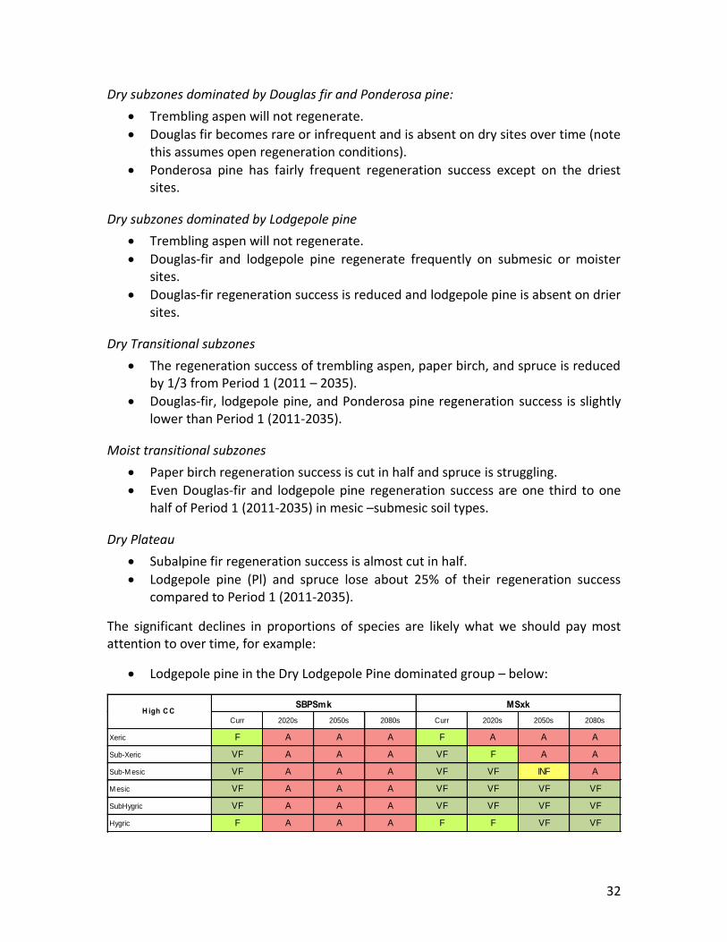
The significant declines in proportions of species are likely what we should pay most attention to over time, for example:
Lodgepole pine in the Dry Lodgepole Pine dominated group – below:
Curr 2020s 2050s 2080s Curr 2020s 2050s 2080s
Xeric F A A A F A A A
Sub-Xeric VF A A A VF F A A
Sub-M esic VF A A A VF VF INF A
M esic VF A A A VF VF VF VF
SubHygric VF A A A VF VF VF VF
Hygric F A A A F F VF VF
SBPSmk MSxkH igh C C
33
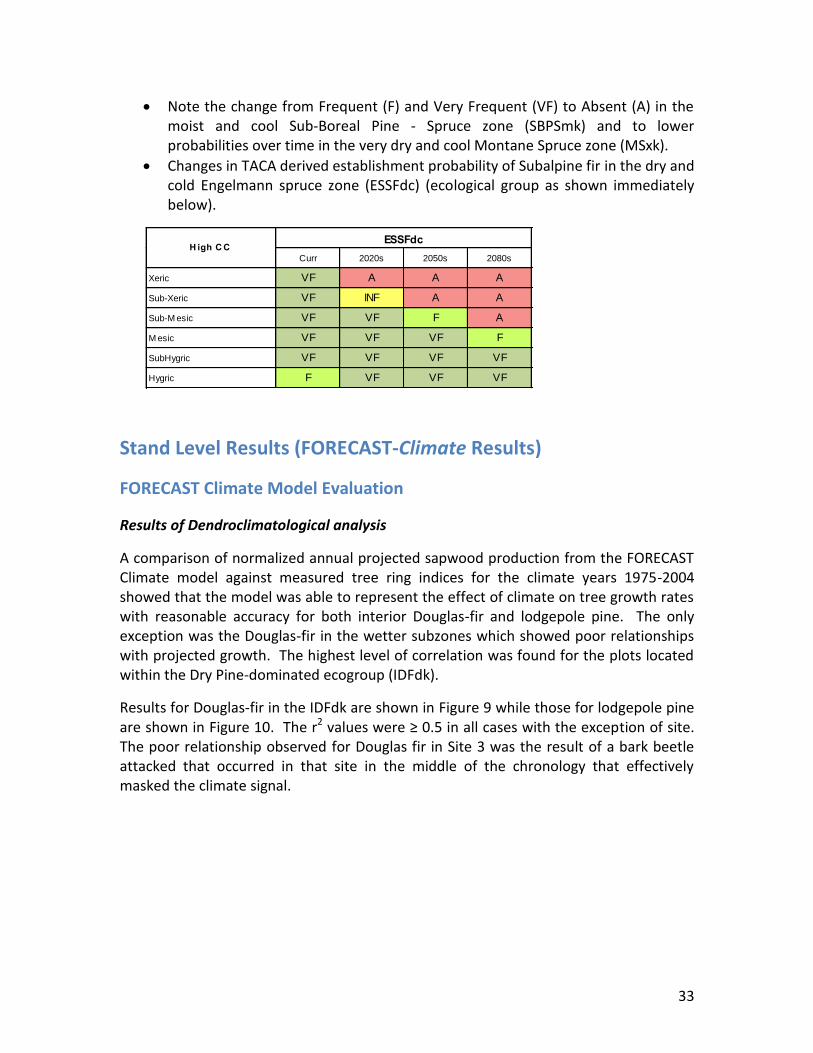
Note the change from Frequent (F) and Very Frequent (VF) to Absent (A) in the moist and cool Sub-Boreal Pine - Spruce zone (SBPSmk) and to lower probabilities over time in the very dry and cool Montane Spruce zone (MSxk).
Changes in TACA derived establishment probability of Subalpine fir in the dry and cold Engelmann spruce zone (ESSFdc) (ecological group as shown immediately below).
Stand Level Results (FORECAST-Climate Results)
FORECAST Climate Model Evaluation
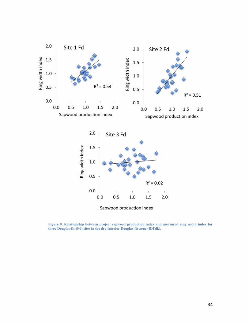
Results of Dendroclimatological analysis
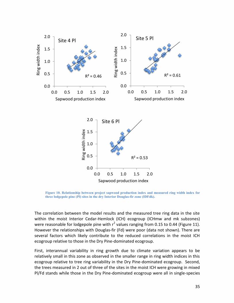
A comparison of normalized annual projected sapwood production from the FORECAST Climate model against measured tree ring indices for the climate years 1975-2004 showed that the model was able to represent the effect of climate on tree growth rates with reasonable accuracy for both interior Douglas-fir and lodgepole pine. The only exception was the Douglas-fir in the wetter subzones which showed poor relationships with projected growth. The highest level of correlation was found for the plots located within the Dry Pine-dominated ecogroup (IDFdk).
Results for Douglas-fir in the IDFdk are shown in Figure 9 while those for lodgepole pine are shown in Figure 10. The r2 values were ≥ 0.5 in all cases with the exception of site. The poor relationship observed for Douglas fir in Site 3 was the result of a bark beetle attacked that occurred in that site in the middle of the chronology that effectively masked the climate signal.
Curr 2020s 2050s 2080s
Xeric VF A A A
Sub-Xeric VF INF A A
Sub-M esic VF VF F A
M esic VF VF VF F
SubHygric VF VF VF VF
Hygric F VF VF VF
ESSFdcH igh C C
34
Figure 9. Relationship between project sapwood production index and measured ring width index for three Douglas-fir (Fd) sites in the dry Interior Douglas-fir zone (IDFdk).
R² = 0.54
0.0
0.5
1.0
1.5
2.0
0.0 0.5 1.0 1.5 2.0
Rin
g w
idth
ind
ex
Sapwood production index
Site 1 Fd
R² = 0.51
0.0
0.5
1.0
1.5
2.0
0.0 0.5 1.0 1.5 2.0
Rin
g w
idth
ind
ex
Sapwood production index
Site 2 Fd
R² = 0.02
0.0
0.5
1.0
1.5
2.0
0.0 0.5 1.0 1.5 2.0
Rin
g w
idth
ind
ex
Sapwood production index
Site 3 Fd
35
Figure 10. Relationship between project sapwood production index and measured ring width index for three lodgepole pine (Pl) sites in the dry Interior Douglas-fir zone (IDFdk).
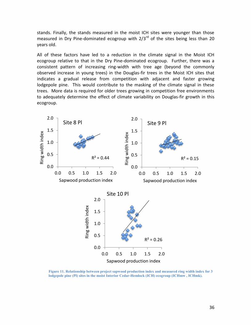
The correlation between the model results and the measured tree ring data in the site within the moist Interior Cedar-Hemlock (ICH) ecogroup (ICHmw and mk subzones) were reasonable for lodgepole pine with r2 values ranging from 0.15 to 0.44 (Figure 11). However the relationships with Douglas-fir (Fd) were poor (data not shown). There are several factors which likely contribute to the reduced correlations in the moist ICH ecogroup relative to those in the Dry Pine-dominated ecogroup.
First, interannual variability in ring growth due to climate variation appears to be relatively small in this zone as observed in the smaller range in ring width indices in this ecogroup relative to tree ring variability in the Dry Pine-dominated ecogroup. Second, the trees measured in 2 out of three of the sites in the moist ICH were growing in mixed Pl/Fd stands while those in the Dry Pine-dominated ecogroup were all in single-species
R² = 0.46
0.0
0.5
1.0
1.5
2.0
0.0 0.5 1.0 1.5 2.0
Rin
g w
idth
ind
ex
Sapwood production index
Site 4 Pl
R² = 0.61
0.0
0.5
1.0
1.5
2.0
0.0 0.5 1.0 1.5 2.0
Rin
g w
idth
ind
ex
Sapwood production index
Site 5 Pl
R² = 0.53
0.0
0.5
1.0
1.5
2.0
0.0 0.5 1.0 1.5 2.0
Rin
g w
idth
ind
ex
Sapwood production index
Site 6 Pl
36
stands. Finally, the stands measured in the moist ICH sites were younger than those measured in Dry Pine-dominated ecogroup with 2/3rd of the sites being less than 20 years old.
All of these factors have led to a reduction in the climate signal in the Moist ICH ecogroup relative to that in the Dry Pine-dominated ecogroup. Further, there was a consistent pattern of increasing ring-width with tree age (beyond the commonly observed increase in young trees) in the Douglas-fir trees in the Moist ICH sites that indicates a gradual release from competition with adjacent and faster growing lodgepole pine. This would contribute to the masking of the climate signal in these trees. More data is required for older trees growing in competition free environments to adequately determine the effect of climate variability on Douglas-fir growth in this ecogroup.
Figure 11. Relationship between project sapwood production index and measured ring width index for 3 lodgepole pine (Pl) sites in the moist Interior Cedar-Hemlock (ICH) ecogroup (ICHmw , ICHmk).
R² = 0.44
0.0
0.5
1.0
1.5
2.0
0.0 0.5 1.0 1.5 2.0
Rin
g w
idth
ind
ex
Sapwood production index
Site 8 Pl
R² = 0.15
0.0
0.5
1.0
1.5
2.0
0.0 0.5 1.0 1.5 2.0
Rin
g w
idth
ind
ex
Sapwood production index
Site 9 Pl
R² = 0.26
0.0
0.5
1.0
1.5
2.0
0.0 0.5 1.0 1.5 2.0
Rin
g w
idth
ind
ex
Sapwood production index
Site 10 Pl
37
General findings – Stand Level Analysis
Description of Nomenclature
In the following section the analysis units (or stand units) are referred to using a numbering system in which they are divided into 3 main groups: 100 series, 200 series, and 300 series. A complete description of the model assumptions for each analysis unit a provided in Appendix 9.
The 100 series analysis units represent existing and future natural stands. The model regeneration assumptions used to represent the analysis units came from a review of the current inventory data in the case of existing stands and were derived from TACA output in the case of future natural stands.
The 200 series analysis units represent existing and future managed stands. The model regeneration assumptions used to represent the analysis units came from a review of the current planting data in the case of existing stands (using the provincial RESULTS database). In the case of future managed stands, output from TACA was used to modify the establishment rate of planted trees.
The 300 series analysis units represent adaptive management strategies for future managed stands. Adaptive management analysis units were created for 7 analysis units. These analysis units were selected for adaptive management as they showed vulnerabilities to climate change based up on TACA survival results and FORECAST stress results (in 200 series stands). Analysis units with small representation in the landbase (<2%) were not selected. Changes to the regeneration choices within selected analysis units included different species choices and in some cases modified planting densities to improve suitability under the climate change scenario.
Period 1 refers stands regenerated between 2010 and 2035
Period 2 refers stands regenerated between 2036 and 2065
Period 3 refers stands regenerated after 2065
Productivity
The results from FORECAST Climate suggest that climate change under the modelled A1B1 scenario will have both positive and negative impacts on stand-level productivity in the K2 project area. The warming of air temperatures generally led to a lengthening of the growing season in all ecozones. In addition, climate warming led to increases in the decomposition of dead organic matter and the associated release of nutrients. Both of these effects had a positive impact on stand-level productivity. In contrast, climate change consistently led to an increase in mid-growing season water stress which had a negative impact on growth rates and often resulted in increased mortality (see below). The net impact of these competing effects on long-term stand productivity depended on
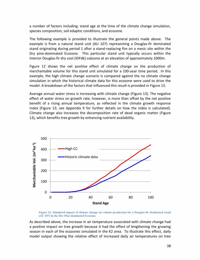
38
a number of factors including: stand age at the time of the climate change simulation, species composition, soil edaphic conditions, and ecozone.
The following example is provided to illustrate the general points made above. The example is from a natural stand unit (AU 107) representing a Douglas-fir dominated stand originating during period 1 after a stand-replacing fire on a mesic site within the Dry pine-dominated Ecozone. This particular stand unit typically occurs within the Interior Douglas-fir dry cool (IDFdk) subzone at an elevation of approximately 1000m.
Figure 12 shows the net positive effect of climate change on the production of merchantable volume for this stand unit simulated for a 100-year time period. In this example, the high climate change scenario is compared against the no climate change simulation in which the historical climate data for this ecozone were used to drive the model. A breakdown of the factors that influenced this result is provided in Figure 13.
Average annual water stress is increasing with climate change (Figure 13). The negative effect of water stress on growth rate, however, is more than offset by the net positive benefit of a rising annual temperature, as reflected in the climate growth response index (Figure 13; see Appendix 9 for further details on how the index is calculated). Climate change also increases the decomposition rate of dead organic matter (Figure 13), which benefits tree growth by enhancing nutrient availability.
Figure 12. Simulated impact of climate change on volume production for a Douglas-fir dominated stand (AU 107) in the Dry Pine-dominated Ecozone.
As described above, the increase in air temperature associated with climate change had a positive impact on tree growth because it had the effect of lengthening the growing season in each of the ecozones simulated in the K2 area. To illustrate this effect, daily model output showing the relative effect of increased daily air temperatures on tree
0
100
200
300
400
500
0 20 40 60 80 100
Mer
chan
tab
le V
ol.
(m
3 h
a-1)
Stand Age
High CC
Historic climate data
39
growth are shown for two representative years for AU 107 ( a good growth year and a poor growth year) in Figure 14. In this case a ‘good’ year is defined as a year in which the climate growth response index (Figure 13), simulated using the historical climate data, is well above 0 (an average year). In contrast, a ‘poor’ year is defined as a year in which the climate growth response index falls below zero.
The pattern of enhanced growth in the spring and fall due to elevated air temperature (climate change) is clearly shown in both years with an average annual increase in the temperature feedback on growth rates of 37% to 42%. In contrast, climate change had a negative impact on the moisture availability feedback on growth rates for both of the representative years (Figure 14). Interestingly, there was a stronger negative feedback from climate change in the good growth year (-20% annually) compared to the poor growth year (-8% annually).
The reason for the stronger negative effect in the good year is that climate change appeared to transform a year with little water stress to a year with substantial water stress. In the case of the poor growth year, growth was already being restricted by water stress in this year so additional stress had a smaller impact. The combined net effect of the daily temperature and moisture availability feedback to growth are shown for the same representative years in Figure 14. In this case climate change had a net positive impact in the poor growth year (+ 37%) and a smaller net negative impact in the good (- 10%) growth year.
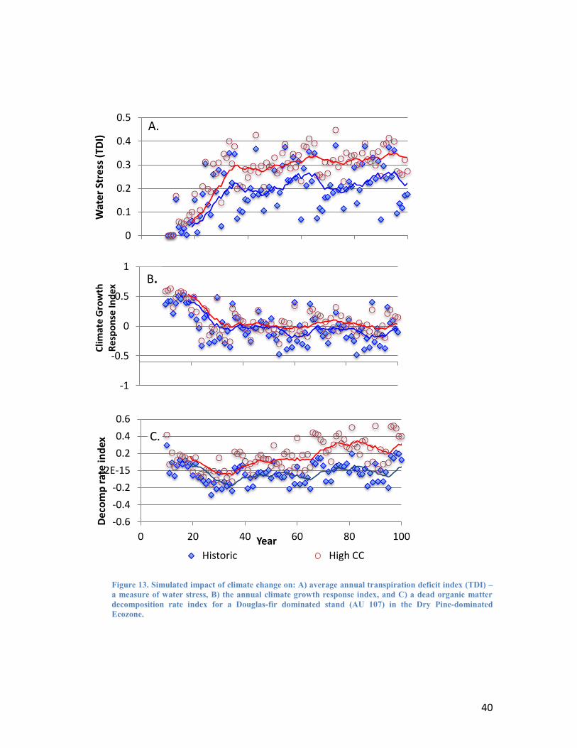
40
Figure 13. Simulated impact of climate change on: A) average annual transpiration deficit index (TDI) – a measure of water stress, B) the annual climate growth response index, and C) a dead organic matter decomposition rate index for a Douglas-fir dominated stand (AU 107) in the Dry Pine-dominated Ecozone.
0
0.1
0.2
0.3
0.4
0.5
Wat
er S
tres
s (T
DI)
A.
-1
-0.5
0
0.5
1
Clim
ate
Gro
wth
R
esp
on
se In
de
x
B.
-0.6
-0.4
-0.2
-2E-15
0.2
0.4
0.6
0 20 40 60 80 100
Dec
om
p r
ate
ind
ex
Year
Historic High CC
C.
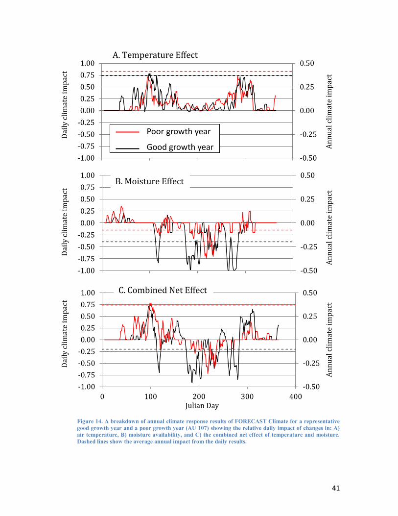
41
Figure 14. A breakdown of annual climate response results of FORECAST Climate for a representative good growth year and a poor growth year (AU 107) showing the relative daily impact of changes in: A) air temperature, B) moisture availability, and C) the combined net effect of temperature and moisture. Dashed lines show the average annual impact from the daily results.
-0.50
-0.25
0.00
0.25
0.50
-1.00
-0.75
-0.50
-0.25
0.00
0.25
0.50
0.75
1.00
An
nu
al c
lim
ate
imp
act
Dai
ly c
lim
ate
imp
act
A. Temperature Effect
-0.50
-0.25
0.00
0.25
0.50
-1.00
-0.75
-0.50
-0.25
0.00
0.25
0.50
0.75
1.00
An
nu
al c
lim
ate
imp
act
Dai
ly c
lim
ate
imp
act
B. Moisture Effect
-0.50
-0.25
0.00
0.25
0.50
-1.00
-0.75
-0.50
-0.25
0.00
0.25
0.50
0.75
1.00
0 100 200 300 400
An
nu
al c
lim
ate
imp
act
Dai
ly c
lim
ate
imp
act
Julian Day
C. Combined Net Effect
Poor growth year
Good growth year
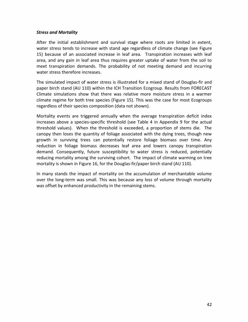
42
Stress and Mortality
After the initial establishment and survival stage where roots are limited in extent, water stress tends to increase with stand age regardless of climate change (see Figure 15) because of an associated increase in leaf area. Transpiration increases with leaf area, and any gain in leaf area thus requires greater uptake of water from the soil to meet transpiration demands. The probability of not meeting demand and incurring water stress therefore increases.
The simulated impact of water stress is illustrated for a mixed stand of Douglas-fir and paper birch stand (AU 110) within the ICH Transition Ecogroup. Results from FORECAST Climate simulations show that there was relative more moisture stress in a warmer climate regime for both tree species (Figure 15). This was the case for most Ecogroups regardless of their species composition (data not shown).
Mortality events are triggered annually when the average transpiration deficit index increases above a species-specific threshold (see Table 4 in Appendix 9 for the actual threshold values). When the threshold is exceeded, a proportion of stems die. The canopy then loses the quantity of foliage associated with the dying trees, though new growth in surviving trees can potentially restore foliage biomass over time. Any reduction in foliage biomass decreases leaf area and lowers canopy transpiration demand. Consequently, future susceptibility to water stress is reduced, potentially reducing mortality among the surviving cohort. The impact of climate warming on tree mortality is shown in Figure 16, for the Douglas-fir/paper birch stand (AU 110).
In many stands the impact of mortality on the accumulation of merchantable volume over the long-term was small. This was because any loss of volume through mortality was offset by enhanced productivity in the remaining stems.
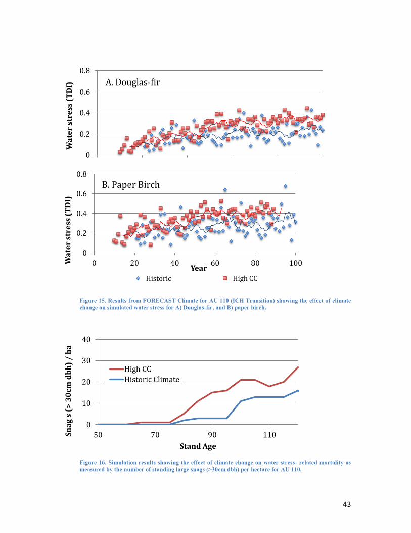
43
Figure 15. Results from FORECAST Climate for AU 110 (ICH Transition) showing the effect of climate change on simulated water stress for A) Douglas-fir, and B) paper birch.
Figure 16. Simulation results showing the effect of climate change on water stress- related mortality as measured by the number of standing large snags (>30cm dbh) per hectare for AU 110.
0
0.2
0.4
0.6
0.8 W
ate
r st
ress
(T
DI)
A. Douglas-fir
0
0.2
0.4
0.6
0.8
0 20 40 60 80 100 Wa
ter
stre
ss (
TD
I)
Year
B. Paper Birch
Historic High CC
0
10
20
30
40
50 70 90 110 Sn
ag
s (
> 3
0cm
db
h)
/ h
a
Stand Age
High CC
Historic Climate
44
Results by Ecozone
The following section provides a description of the stand-level results from the FORECAST Climate analysis summarized by ecozone. For each ecozone, a general description of the impact of climate change on future productivity, moisture stress, and mortality is provided.
Dry Fir-Dominated Ecozone
Projected Impact of Climate Change on Productivity:
The relative impact of climate change on stand-level volume production is shown for analysis units within the Dry Fir-dominated Ecozone for existing (Table 6), and future stands (Table 7). The following trends were observed:
Existing stands
Volume production in stands less than 40 years of age at the start of the simulation showed the most positive impact of climate change, particularly after 50 years of growth. In most cases, relative productivity declined as stands aged from 50 to 100 years old.
Volume production in stands more than 80 years old at the start of the simulation were largely unaffected by climate change.
Mortality rates increased with climate change in nearly all stand units leading to greater numbers of large (>30ch dbh) snags and logs (data not shown).
Aspen suffered higher mortality under climate change (data not shown.
Future stands
Stands regenerating in Period 1 (2010-2035) showed increased productivity under climate change, particularly within the first 50 years of growth. In most cases, relative productivity declined as stands aged from 50 to 100 years old, regardless of which period stands were regenerated.
The negative impact of climate change on volume production tended to become more pronounced between periods 2 (2036-2065) and 3 (> 2065).
Increases in productivity (at a given age) were usually lower in Period 3 relative to period 2.
Stands regenerating in periods 2 (2036-2065) and 3 (> 2065) often showed reduced densities related to higher rates of mortality during the establishment phase (data not shown).
Reduced stand densities actually reduce water stress in maturing stands by reducing leaf area (data not shown).
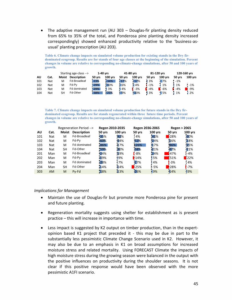
45
The adaptive management run (AU 303 – Douglas-fir planting density reduced from 65% to 35% of the total, and Ponderosa pine planting density increased correspondingly) showed enhanced productivity relative to the ‘business-as-usual’ planting prescription (AU 203).
Table 6. Climate change impacts on simulated volume production for existing stands in the Dry fir-dominated ecogroup. Results are for stands of four age classes at the beginning of the simulation. Percent changes in volume are relative to corresponding no-climate-change simulations, after 50 and 100 years of growth.
Table 7. Climate change impacts on simulated volume production for future stands in the Dry fir-dominated ecogroup. Results are for stands regenerated within three future time periods. Percent changes in volume are relative to corresponding no-climate-change simulations, after 50 and 100 years of growth.
Implications for Management
Maintain the use of Douglas-fir but promote more Ponderosa pine for present and future planting.
Regeneration mortality suggests using shelter for establishment as is present practice – this will increase in importance with time.
Less impact is suggested by K2 output on timber production, than in the expert-opinion based K1 project that preceded it - this may be due in part to the substantially less pessimistic Climate Change Scenario used in K2. However, it may also be due to an emphasis in K1 on broad assumptions for increased moisture stress and related mortality. Using FORECAST Climate the impacts of high moisture stress during the growing season were balanced in the output with the positive influences on productivity during the shoulder seasons. It is not clear if this positive response would have been observed with the more pessimistic A1FI scenario.
AU Cat. Moist Description 50yrs 100yrs 50yrs 100yrs 50yrs 100yrs 50yrs 100yrs101 Nat M Fd-Broadleaf 23% 34% 17% 17% 3% 7% -1%102 Nat M Fd-Py 29% 10% 6% 4% -1% 1% 1% -1%103 Nat M Fd dominated 29% 3% 4% -3% -4% -6% -4% -9%104 Nat SH Fd-Other 38% 21% 9% 10% 3% 5% 1% 2%
Startingage-class--> 120-160yrs1-40yrs 41-80yrs 81-120yrs
AU Cat. Moist Description 50yrs 100yrs 50yrs 100yrs 50yrs 100yrs101 Nat M Fd-Broadleaf 35% 42% 4% 41% -28% 30%102 Nat M Fd-Py 60% 24% 52% 24% 16% 18%103 Nat M Fd dominated 86% 17% 126% 17% 86% 25%104 Nat SH Fd-Other 59% 30% 58% 21% 37% 21%201 Man M Fd-Broadleaf 24% 19% -8% 24% -47% -4%202 Man M Fd-Py 19% 9% -14% 5% -51% -22%203 Man M Fd dominated 28% 7% 27% 4% -3% 4%204 Man SH Fd-Other 14% 14% -25% -5% -28% -7%
303 AM M Py-Fd 18% 13% 26% 9% 14% 9%
RegenerationPeriod--> Regen2010-2035 Regen2036-2065 Regen>2065
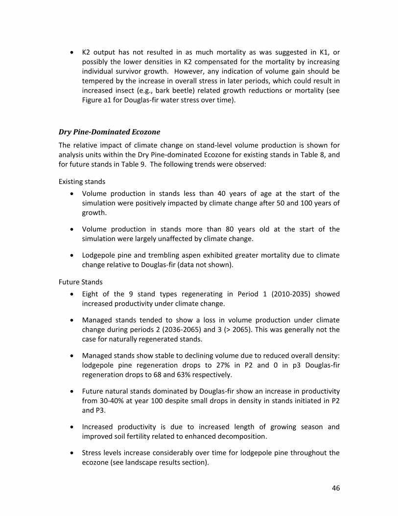
46
K2 output has not resulted in as much mortality as was suggested in K1, or possibly the lower densities in K2 compensated for the mortality by increasing individual survivor growth. However, any indication of volume gain should be tempered by the increase in overall stress in later periods, which could result in increased insect (e.g., bark beetle) related growth reductions or mortality (see Figure a1 for Douglas-fir water stress over time).
Dry Pine-Dominated Ecozone
The relative impact of climate change on stand-level volume production is shown for analysis units within the Dry Pine-dominated Ecozone for existing stands in Table 8, and for future stands in Table 9. The following trends were observed:
Existing stands
Volume production in stands less than 40 years of age at the start of the simulation were positively impacted by climate change after 50 and 100 years of growth.
Volume production in stands more than 80 years old at the start of the simulation were largely unaffected by climate change.
Lodgepole pine and trembling aspen exhibited greater mortality due to climate change relative to Douglas-fir (data not shown).
Future Stands
Eight of the 9 stand types regenerating in Period 1 (2010-2035) showed increased productivity under climate change.
Managed stands tended to show a loss in volume production under climate change during periods 2 (2036-2065) and 3 (> 2065). This was generally not the case for naturally regenerated stands.
Managed stands show stable to declining volume due to reduced overall density: lodgepole pine regeneration drops to 27% in P2 and 0 in p3 Douglas-fir regeneration drops to 68 and 63% respectively.
Future natural stands dominated by Douglas-fir show an increase in productivity from 30-40% at year 100 despite small drops in density in stands initiated in P2 and P3.
Increased productivity is due to increased length of growing season and improved soil fertility related to enhanced decomposition.
Stress levels increase considerably over time for lodgepole pine throughout the ecozone (see landscape results section).
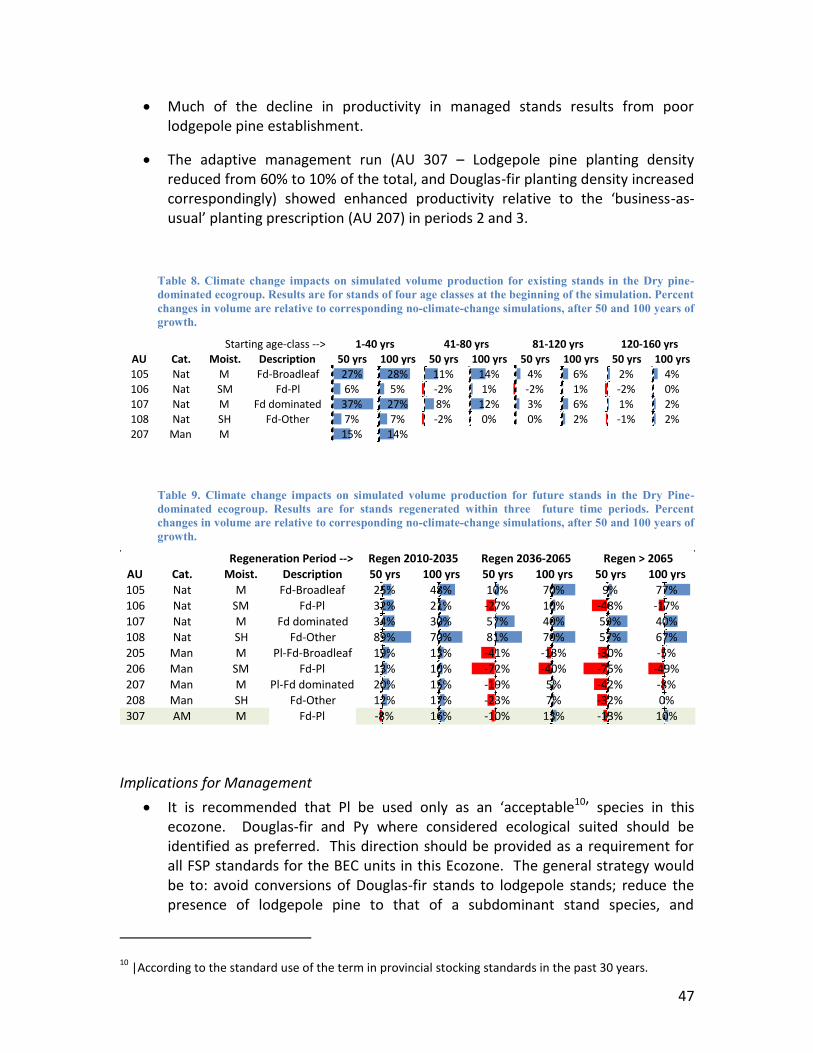
47
Much of the decline in productivity in managed stands results from poor lodgepole pine establishment.
The adaptive management run (AU 307 – Lodgepole pine planting density reduced from 60% to 10% of the total, and Douglas-fir planting density increased correspondingly) showed enhanced productivity relative to the ‘business-as-usual’ planting prescription (AU 207) in periods 2 and 3.
Table 8. Climate change impacts on simulated volume production for existing stands in the Dry pine-dominated ecogroup. Results are for stands of four age classes at the beginning of the simulation. Percent changes in volume are relative to corresponding no-climate-change simulations, after 50 and 100 years of growth.
Table 9. Climate change impacts on simulated volume production for future stands in the Dry Pine-dominated ecogroup. Results are for stands regenerated within three future time periods. Percent changes in volume are relative to corresponding no-climate-change simulations, after 50 and 100 years of growth.
Implications for Management
It is recommended that Pl be used only as an ‘acceptable10’ species in this ecozone. Douglas-fir and Py where considered ecological suited should be identified as preferred. This direction should be provided as a requirement for all FSP standards for the BEC units in this Ecozone. The general strategy would be to: avoid conversions of Douglas-fir stands to lodgepole stands; reduce the presence of lodgepole pine to that of a subdominant stand species, and
10 |According to the standard use of the term in provincial stocking standards in the past 30 years.
AU Cat. Moist. Description 50yrs 100yrs 50yrs 100yrs 50yrs 100yrs 50yrs 100yrs
105 Nat M Fd-Broadleaf 27% 28% 11% 14% 4% 6% 2% 4%106 Nat SM Fd-Pl 6% 5% -2% 1% -2% 1% -2% 0%
107 Nat M Fddominated 37% 27% 8% 12% 3% 6% 1% 2%108 Nat SH Fd-Other 7% 7% -2% 0% 0% 2% -1% 2%
207 Man M 15% 14%
Startingage-class--> 120-160yrs1-40yrs 41-80yrs 81-120yrs
AU Cat. Moist. Description 50yrs 100yrs 50yrs 100yrs 50yrs 100yrs
105 Nat M Fd-Broadleaf 25% 48% 10% 70% 9% 77%106 Nat SM Fd-Pl 32% 21% -27% 10% -48% -17%107 Nat M Fddominated 34% 30% 57% 40% 59% 40%108 Nat SH Fd-Other 89% 70% 81% 70% 57% 67%205 Man M Pl-Fd-Broadleaf 19% 13% -41% -13% -30% -5%206 Man SM Fd-Pl 13% 10% -72% -40% -75% -49%
207 Man M Pl-Fddominated 20% 15% -19% 5% -42% -8%208 Man SH Fd-Other 12% 17% -23% 7% -32% 0%307 AM M Fd-Pl -8% 16% -10% 13% -13% 10%
RegenerationPeriod--> Regen2010-2035 Regen2036-2065 Regen>2065
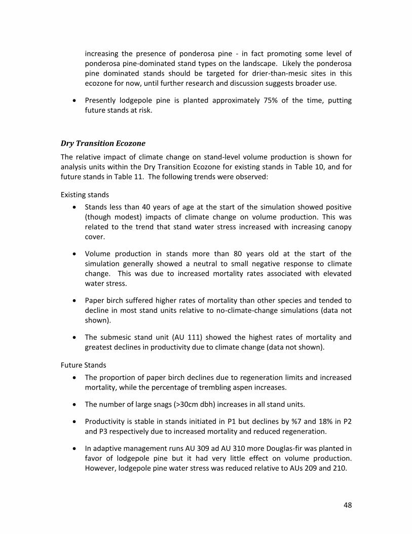
48
increasing the presence of ponderosa pine - in fact promoting some level of ponderosa pine-dominated stand types on the landscape. Likely the ponderosa pine dominated stands should be targeted for drier-than-mesic sites in this ecozone for now, until further research and discussion suggests broader use.
Presently lodgepole pine is planted approximately 75% of the time, putting future stands at risk.
Dry Transition Ecozone
The relative impact of climate change on stand-level volume production is shown for analysis units within the Dry Transition Ecozone for existing stands in Table 10, and for future stands in Table 11. The following trends were observed:
Existing stands
Stands less than 40 years of age at the start of the simulation showed positive (though modest) impacts of climate change on volume production. This was related to the trend that stand water stress increased with increasing canopy cover.
Volume production in stands more than 80 years old at the start of the simulation generally showed a neutral to small negative response to climate change. This was due to increased mortality rates associated with elevated water stress.
Paper birch suffered higher rates of mortality than other species and tended to decline in most stand units relative to no-climate-change simulations (data not shown).
The submesic stand unit (AU 111) showed the highest rates of mortality and greatest declines in productivity due to climate change (data not shown).
Future Stands
The proportion of paper birch declines due to regeneration limits and increased mortality, while the percentage of trembling aspen increases.
The number of large snags (>30cm dbh) increases in all stand units.
Productivity is stable in stands initiated in P1 but declines by %7 and 18% in P2 and P3 respectively due to increased mortality and reduced regeneration.
In adaptive management runs AU 309 ad AU 310 more Douglas-fir was planted in favor of lodgepole pine but it had very little effect on volume production. However, lodgepole pine water stress was reduced relative to AUs 209 and 210.
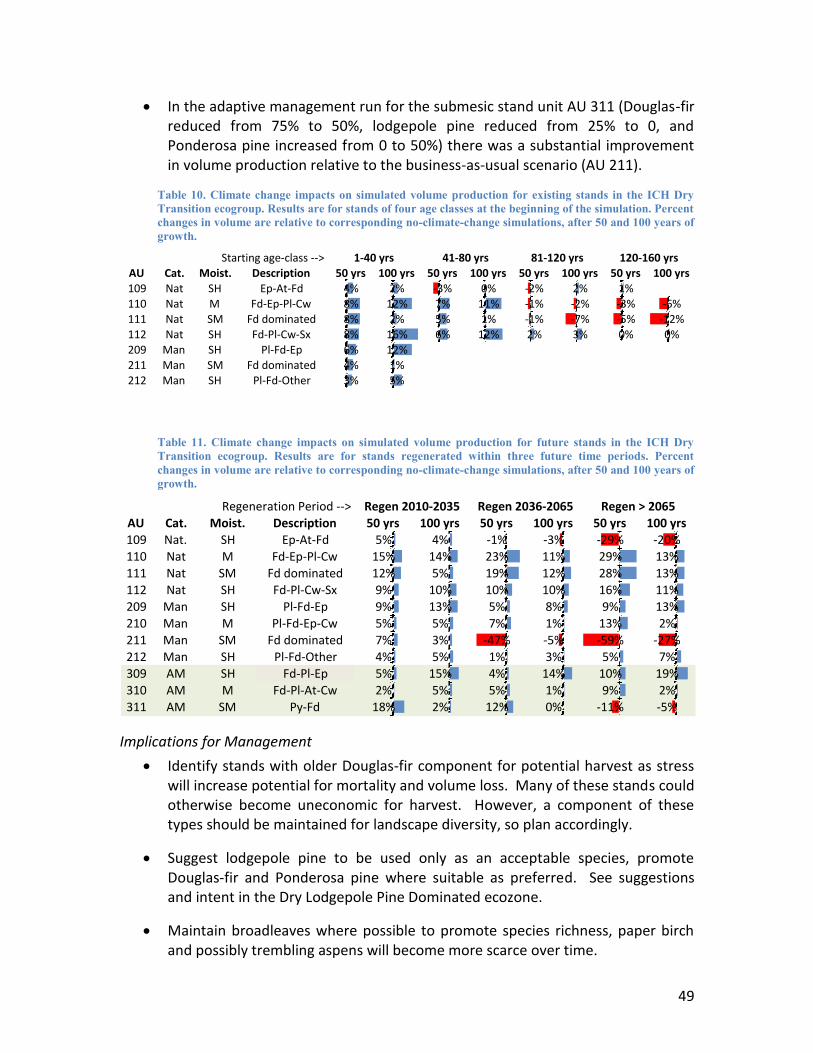
49
In the adaptive management run for the submesic stand unit AU 311 (Douglas-fir reduced from 75% to 50%, lodgepole pine reduced from 25% to 0, and Ponderosa pine increased from 0 to 50%) there was a substantial improvement in volume production relative to the business-as-usual scenario (AU 211).
Table 10. Climate change impacts on simulated volume production for existing stands in the ICH Dry Transition ecogroup. Results are for stands of four age classes at the beginning of the simulation. Percent changes in volume are relative to corresponding no-climate-change simulations, after 50 and 100 years of growth.
Table 11. Climate change impacts on simulated volume production for future stands in the ICH Dry Transition ecogroup. Results are for stands regenerated within three future time periods. Percent changes in volume are relative to corresponding no-climate-change simulations, after 50 and 100 years of growth.
Implications for Management
Identify stands with older Douglas-fir component for potential harvest as stress will increase potential for mortality and volume loss. Many of these stands could otherwise become uneconomic for harvest. However, a component of these types should be maintained for landscape diversity, so plan accordingly.
Suggest lodgepole pine to be used only as an acceptable species, promote Douglas-fir and Ponderosa pine where suitable as preferred. See suggestions and intent in the Dry Lodgepole Pine Dominated ecozone.
Maintain broadleaves where possible to promote species richness, paper birch and possibly trembling aspens will become more scarce over time.
AU Cat. Moist. Description 50yrs 100yrs 50yrs 100yrs 50yrs 100yrs 50yrs 100yrs
109 Nat SH Ep-At-Fd 4% 2% -3% 0% -2% 2% 1%
110 Nat M Fd-Ep-Pl-Cw 8% 12% 7% 11% -1% -2% -3% -6%111 Nat SM Fddominated 8% 2% 5% 1% -1% -7% -5% -12%
112 Nat SH Fd-Pl-Cw-Sx 8% 16% 6% 12% 2% 3% 0% 0%
209 Man SH Pl-Fd-Ep 6% 12%
211 Man SM Fddominated 4% 1%212 Man SH Pl-Fd-Other 3% 5%
Startingage-class--> 120-160yrs1-40yrs 41-80yrs 81-120yrs
AU Cat. Moist. Description 50yrs 100yrs 50yrs 100yrs 50yrs 100yrs
109 Nat. SH Ep-At-Fd 5% 4% -1% -3% -29% -20%
110 Nat M Fd-Ep-Pl-Cw 15% 14% 23% 11% 29% 13%
111 Nat SM Fddominated 12% 5% 19% 12% 28% 13%
112 Nat SH Fd-Pl-Cw-Sx 9% 10% 10% 10% 16% 11%209 Man SH Pl-Fd-Ep 9% 13% 5% 8% 9% 13%
210 Man M Pl-Fd-Ep-Cw 5% 5% 7% 1% 13% 2%
211 Man SM Fddominated 7% 3% -47% -5% -59% -27%
212 Man SH Pl-Fd-Other 4% 5% 1% 3% 5% 7%309 AM SH Fd-Pl-Ep 5% 15% 4% 14% 10% 19%
310 AM M Fd-Pl-At-Cw 2% 5% 5% 1% 9% 2%
311 AM SM Py-Fd 18% 2% 12% 0% -11% -5%
RegenerationPeriod--> Regen2010-2035 Regen2036-2065 Regen>2065
50
ICH Moist transition Ecozone
The relative impact of climate change on stand-level volume production is shown for analysis units within the ICH Moist transition Ecozone for existing stands in Table 12, and for future stands in Table 13. The following trends were observed:
Existing stands
Stands that were less than 40 years of age at the start of the simulation showed positive impacts of climate change after both 50 and 100 years of growth. This was related to the trend that stand water stress increased with increasing canopy cover. Young stands are able to benefit from growth during the early period before water stress gets too high.
Stands greater than 40 years at the start of the simulation generally showed a negative response to climate change that was more pronounced than in the Dry ICH transition. This was attributed to the frequency of warm dry water stress years that were relatively infrequent within this ecozone in the past and that many of the species common in this ecozone are not well adapted to water stress.
There is a considerable increase in large (>30cm dbh) snags and logs throughout the stand units within this ecozone due to increased water stress-related mortality.
Paper birch, spruce and western red cedar were particularly vulnerable to increased water stress.
Future Stands
Most of the future managed stands showed increased volume production with climate change, regardless of the regeneration period.
Modifying the species composition in AU214 (and generating AU314) did not improve volume production but there was an improvement when the Douglas-fir planting density was increased relative to spruce (cf. AU216 versus AU316).
Lodgepole pine was vulnerable to water stress on submesic sites.
Spruce was vulnerable to water stress on both mesic and subhygric sites.
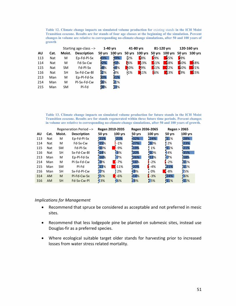
51
Table 12. Climate change impacts on simulated volume production for existing stands in the ICH Moist Transition ecozone. Results are for stands of four age classes at the beginning of the simulation. Percent changes in volume are relative to corresponding no-climate-change simulations, after 50 and 100 years of growth
Table 13. Climate change impacts on simulated volume production for future stands in the ICH Moist Transition ecozone. Results are for stands regenerated within three future time periods. Percent changes in volume are relative to corresponding no-climate-change simulations, after 50 and 100 years of growth.
Implications for Management
Recommend that spruce be considered as acceptable and not preferred in mesic sites.
Recommend that less lodgepole pine be planted on submesic sites, instead use Douglas-fir as a preferred species.
Where ecological suitable target older stands for harvesting prior to increased losses from water stress related mortality.
AU Cat. Moist. Description 50yrs 100yrs 50yrs 100yrs 50yrs 100yrs 50yrs 100yrs
113 Nat M Ep-Fd-Pl-Sx 43% 39% -2% -8% -9% -15% -9%
114 Nat M Fd-Sx-Cw 32% 21% -6% -13% -11% -18% -10% -18%115 Nat SM Fd-Pl-Sx 18% 14% -10% -9% -11% -22% -10% -21%
116 Nat SH Sx-Fd-Cw-Bl 12% 3% -1% -11% -6% -13% -9% -15%
213 Man M Ep-Pl-Fd-Sx 30% 31%
214 Man M Pl-Sx-Fd-Cw 16% 11%215 Man SM Pl-Fd 18% 13%
Startingage-class--> 120-160yrs1-40yrs 41-80yrs 81-120yrs
AU Cat. Moist. Description 50yrs 100yrs 50yrs 100yrs 50yrs 100yrs
113 Nat M Ep-Fd-Pl-Sx 21% 21% 32% 24% 11% 28%114 Nat M Fd-Sx-Cw 15% -1% 27% 10% 2% 23%
115 Nat SM Fd-Pl-Sx 10% -9% 19% 1% 11% 21%
116 Nat SH Sx-Fd-Cw-Bl 14% 8% 20% 10% 4% 35%
213 Man M Ep-Pl-Fd-Sx 16% 7% 26% 13% 7% 18%214 Man M Pl-Sx-Fd-Cw 8% -7% 16% -2% -2% 11%
215 Man SM Pl-Fd 13% -11% 20% -4% 21% 11%
216 Man SH Sx-Fd-Pl-Cw 7% 2% 9% 0% -8% 5%
314 AM M Pl-Fd-Cw-Sx 5% -6% 14% -3% 24% 6%316 AM SH Fd-Sx-Cw-Pl 3% 6% 8% 5% 11% 11%
RegenerationPeriod--> Regen2010-2035 Regen2036-2065 Regen>2065
52
Dry Plateau Ecozone
The relative impact of climate change on stand-level volume production is shown for analysis units within the Dry Plateau Ecozone for existing stands in Table 14, and for future stands in Table 15.
The following trends were observed:
Existing stands
Productivity is projected to increase substantially (40-90%) in these stands (particularly in the wetter regions). This is attributed to a substantial lengthening of growing season with only minor increases in water stress.
Water stress can be a problem in dry years but the frequency of dry years (even with climate change) is low.
Younger existing stands showed the greatest relative increase in volume production and oldest stands showed the smallest.
Snag levels show only small increases due to CC.
Litter decomposition rate index increases by 60 to 110% due to climate change. Dry years don’t increase as much as wet years.
Future stands
Volume production was much improved with climate change (sometimes dramatically) regardless of stand age or regeneration period. Typically, however, yield increases were less in 100 year-old stands, as compared to 50 years old.
Projected increases in yields should be treated with caution as their may also be increases in the activity of biological disturbance agents.
Water stress may be a factor in some areas. It should be pointed out that the climate data for this ecozone was based upon the Sun Peaks climate station which represents a wetter sub-region of the Dry plateau Ecozone.
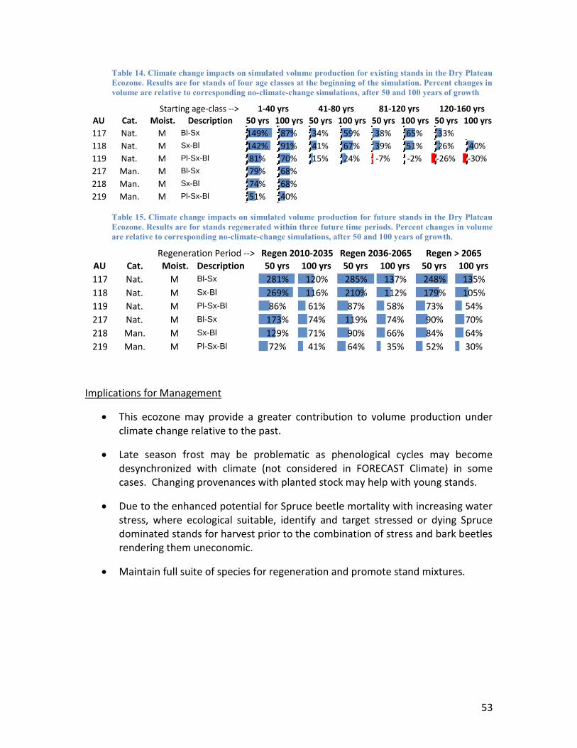
53
Table 14. Climate change impacts on simulated volume production for existing stands in the Dry Plateau Ecozone. Results are for stands of four age classes at the beginning of the simulation. Percent changes in volume are relative to corresponding no-climate-change simulations, after 50 and 100 years of growth
Table 15. Climate change impacts on simulated volume production for future stands in the Dry Plateau Ecozone. Results are for stands regenerated within three future time periods. Percent changes in volume are relative to corresponding no-climate-change simulations, after 50 and 100 years of growth.
Implications for Management
This ecozone may provide a greater contribution to volume production under climate change relative to the past.
Late season frost may be problematic as phenological cycles may become desynchronized with climate (not considered in FORECAST Climate) in some cases. Changing provenances with planted stock may help with young stands.
Due to the enhanced potential for Spruce beetle mortality with increasing water stress, where ecological suitable, identify and target stressed or dying Spruce dominated stands for harvest prior to the combination of stress and bark beetles rendering them uneconomic.
Maintain full suite of species for regeneration and promote stand mixtures.
AU Cat. Moist. Description 50yrs 100yrs 50yrs 100yrs 50yrs 100yrs 50yrs 100yrs
117 Nat. M Bl-Sx 149% 87% 34% 59% 38% 65% 33%
118 Nat. M Sx-Bl 142% 91% 41% 67% 39% 51% 26% 40%
119 Nat. M Pl-Sx-Bl 81% 70% 15% 24% -7% -2% -26% -30%
217 Man. M Bl-Sx 79% 68%
218 Man. M Sx-Bl 74% 68%
219 Man. M Pl-Sx-Bl 51% 40%
Startingage-class--> 120-160yrs1-40yrs 41-80yrs 81-120yrs
AU Cat. Moist. Description 50yrs 100yrs 50yrs 100yrs 50yrs 100yrs
117 Nat. M Bl-Sx 281% 120% 285% 137% 248% 135%
118 Nat. M Sx-Bl 269% 116% 210% 112% 179% 105%
119 Nat. M Pl-Sx-Bl 86% 61% 87% 58% 73% 54%
217 Nat. M Bl-Sx 173% 74% 119% 74% 90% 70%
218 Man. M Sx-Bl 129% 71% 90% 66% 84% 64%
219 Man. M Pl-Sx-Bl 72% 41% 64% 35% 52% 30%
RegenerationPeriod--> Regen2010-2035 Regen2036-2065 Regen>2065

54
Landscape Level Results (FPS and Dyna-Plan Results)
Introduction and Context
The Intent for this Section
The intent of this section is to:
1. Discuss the key trends for the modelling indicators as they apply over the whole study area in general, sometimes focussing on specific ecozones. The Dry and Moist Transitional ecozones are often cited as they are the dominant managed ecozones. However, where other ecozones have unusual trends, these are also discussed.
2. Describe the key considerations for managers based on these trends, and the associated assumptions, uncertainties and approaches used for modelling.
3. Illustrate the type of detailed output data that can be expected from this type of modelling suite with climate change – using the Dry and Moist Transitional Ecozones as examples.
The Landscape Context
In moving from the stand level to the landscape, it is important to restate that the case study area encompasses almost 400,000 ha of productive forest land and is comprised of six ecozones. We modelled climate change across five of these ecozones or 83% of the case study area. The Wet Engelmann Spruce-Subapline Fir ecozone was not modelled due to a lack of climate data to allow for our regional downscaling and calibration. Modelling results from FORECAST for 19 different stand types across these five ecozones provided input data /curves for the two landscape level models used, Forest Planning Studio (FPS) and Dyna-Plan.
Considerations for Managers
Managers interpreting the impact of climate change in the Case Study Area should consider the following:
The Wet Engelmann Spruce-Subapline Fir ecozone was not modelled for climate change.
The main themes and considerations presented here may be relevant to other management units in BC, especially in the southern Interior, where they should be considered for their applicability. As in all cases with modelling, care should be taken when extrapolating results and conclusions from one area to another to ensure that the ecological and management context as well as the assumptions are appropriate.
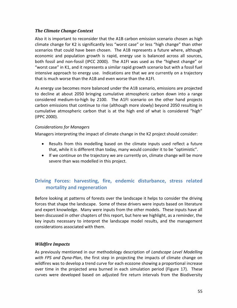
55
The Climate Change Context
Also it is important to reconsider that the A1B carbon emission scenario chosen as high climate change for K2 is significantly less “worst case” or less “high change” than other scenarios that could have been chosen. The A1B represents a future where, although economic and population growth is rapid, energy use is balanced across all sources, both fossil and non-fossil (IPCC 2000). The A1FI was used as the “highest change” or “worst case” in K1, and it represents a similar rapid growth scenario but with a fossil fuel intensive approach to energy use. Indications are that we are currently on a trajectory that is much worse than the A1B and even worse than the A1FI.
As energy use becomes more balanced under the A1B scenario, emissions are projected to decline at about 2050 bringing cumulative atmospheric carbon down into a range considered medium-to-high by 2100. The A1FI scenario on the other hand projects carbon emissions that continue to rise (although more slowly) beyond 2050 resulting in cumulative atmospheric carbon that is at the high end of what is considered “high” (IPPC 2000).
Considerations for Managers
Managers interpreting the impact of climate change in the K2 project should consider:
Results from this modelling based on the climate inputs used reflect a future that, while it is different than today, many would consider it to be “optimistic”.
If we continue on the trajectory we are currently on, climate change will be more severe than was modelled in this project.
Driving Forces: harvesting, fire, endemic disturbance, stress related mortality and regeneration
Before looking at patterns of forests over the landscape it helps to consider the driving forces that shape the landscape. Some of these drivers were inputs based on literature and expert knowledge. Many were inputs from the other models. These inputs have all been discussed in other chapters of this report, but here we highlight, as a reminder, the key inputs necessary to interpret the landscape model results, and the management considerations associated with them.
Wildfire Impacts
As previously mentioned in our methodology description of Landscape Level Modelling with FPS and Dyna-Plan, the first step in projecting the impacts of climate change on wildfires was to develop a trend curve for each ecozone showing a proportional increase over time in the projected area burned in each simulation period (Figure 17). These curves were developed based on adjusted fire return intervals from the Biodiversity
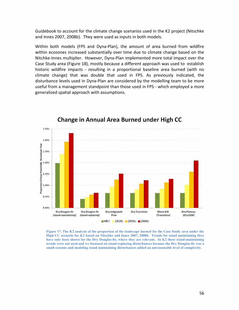
56
Guidebook to account for the climate change scenarios used in the K2 project (Nitschke and Innes 2007, 2008b). They were used as inputs in both models.
Within both models (FPS and Dyna-Plan), the amount of area burned from wildfire within ecozones increased substantially over time due to climate change based on the Nitchke-Innes multiplier. However, Dyna-Plan implemented more total impact over the Case Study area (Figure 18), mostly because a different approach was used to establish historic wildfire impacts - resulting in a proportional baseline area burned (with no climate change) that was double that used in FPS. As previously indicated, the disturbance levels used in Dyna-Plan are considered by the modelling team to be more useful from a management standpoint than those used in FPS - which employed a more generalized spatial approach with assumptions.
Figure 17. The K2 analysis of the proportion of the landscape burned for the Case Study area under the High CC scenario for K2 based on Nitschke and Innes 2007, 2008b. Trends for stand maintaining fires have only been shown for the Dry Douglas-fir, where they are relevant. In K2 these stand-maintaining trends were not used and we focussed on stand-replacing disturbances because the Dry Douglas-fir was a small ecozone and modeling stand maintaining disturbances added an unreasonable level of complexity.
57
Historic fires in the last 90 years, showing the Case study area in context with a larger area (GIS data from GeoBC).
Dyna-Plan Simulation of fires with HCC (All fires for the period of 2020-2110)
Figure 18. Changes in fire patterns over the Case Study area as projected by Dyna-Plan. From the left showing historic patterns over the past 90 years in the Case Study area and the surrounding region, and from the right simulated fires with the high climate change scenario over the next 90 years showing a doubling of fire impacts in that time period.
FPS represented fires with a deterministic approach on the Non-THLB only using a spatially dispersed (random) approach. Dyna-Plan employed a stochastic fire ignition/size approach with a spatially-explicit representation of fire growth patterns.
Considerations for Managers
When designing strategies to manage for climate change over time, managers should consider:
With climate change the impact of wildfire is projected to double over the next 100 years in the Case Study area with a business-as-usual approach to management and fire suppression.
The K2 modeling does simplify impacts on stand conditions from fire by not considering stand maintaining disturbances and generally ignoring within-stand patches that would be skipped during stand replacing fires. Some would say that the general impacts from fire (particularly those from Dyna-Plan) may therefore be overstated.
o However, it should be remembered that K2 did not model stand-replacing disturbances from insect epidemics, which could add significantly more disturbance over the simulation period.
The Dyna-Plan results therefore may illustrate a surprising amount of disturbance over the next 100 years, however this may be quite plausible in light of what we know about climate change and potential risks and uncertainties associated with it.
o Accordingly, the reported future forest conditions in Dyna-Plan should be carefully considered by managers when reviewing results for the subsections that follow. It would be prudent to consider the implications of the Dyna-Plan fire regimes as a plausible future, and plan harvest
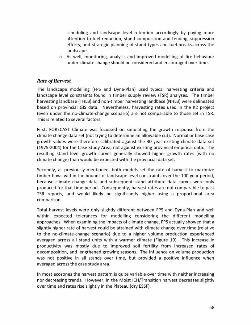
58
scheduling and landscape level retention accordingly by paying more attention to fuel reduction, stand composition and tending, suppression efforts, and strategic planning of stand types and fuel breaks across the landscape.
o As well, monitoring, analysis and improved modelling of fire behaviour under climate change should be considered and encouraged over time.
Rate of Harvest
The landscape modelling (FPS and Dyna-Plan) used typical harvesting criteria and landscape level constraints found in timber supply review (TSR) analyses. The timber harvesting landbase (THLB) and non-timber harvesting landbase (NHLB) were delineated based on provincial GIS data. Nevertheless, harvesting rates used in the K2 project (even under the no-climate-change scenario) are not comparable to those set in TSR. This is related to several factors.
First, FORECAST Climate was focussed on simulating the growth response from the climate change data set (not trying to determine an allowable cut). Normal or base case growth values were therefore calibrated against the 30 year existing climate data set (1975-2004) for the Case Study Area, not against existing provincial empirical data. The resulting stand level growth curves generally showed higher growth rates (with no climate change) than would be expected with the provincial data set.
Secondly, as previously mentioned, both models set the rate of harvest to maximize timber flows within the bounds of landscape level constraints over the 100 year period, because climate change data and subsequent stand attribute data curves were only produced for that time period. Consequently, harvest rates are not comparable to past TSR reports, and would likely be significantly higher using a proportional area comparison.
Total harvest levels were only slightly different between FPS and Dyna-Plan and well within expected tolerances for modelling considering the different modelling approaches. When examining the impacts of climate change, FPS actually showed that a slightly higher rate of harvest could be attained with climate change over time (relative to the no-climate-change scenario) due to a higher volume production experienced averaged across all stand units with a warmer climate (Figure 19). This increase in productivity was mostly due to improved soil fertility from increased rates of decomposition, and lengthened growing seasons. The influence on volume production was not positive in all stands over time, but provided a positive influence when averaged across the case study area.
In most ecozones the harvest pattern is quite variable over time with neither increasing nor decreasing trends. However, in the Moist ICH/Transition harvest decreases slightly over time and rates rise slightly in the Plateau (dry ESSF).
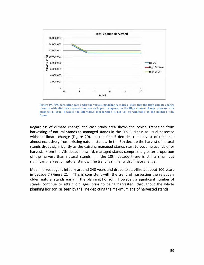
59
Figure 19. FPS harvesting rate under the various modeling scenarios. Note that the High climate change scenario with alternate regeneration has no impact compared to the High climate change basecase with business as usual because the alternative regeneration is not yet merchantable in the modeled time frame.
Regardless of climate change, the case study area shows the typical transition from harvesting of natural stands to managed stands in the FPS Business-as-usual basecase without climate change (Figure 20). In the first 5 decades the harvest of timber is almost exclusively from existing natural stands. In the 6th decade the harvest of natural stands drops significantly as the existing managed stands start to become available for harvest. From the 7th decade onward, managed stands comprise a greater proportion of the harvest than natural stands. In the 10th decade there is still a small but significant harvest of natural stands. The trend is similar with climate change.
Mean harvest age is initially around 240 years and drops to stabilize at about 100 years in decade 7 (Figure 21). This is consistent with the trend of harvesting the relatively older, natural stands early in the planning horizon. However, a significant number of stands continue to attain old ages prior to being harvested, throughout the whole planning horizon, as seen by the line depicting the maximum age of harvested stands.
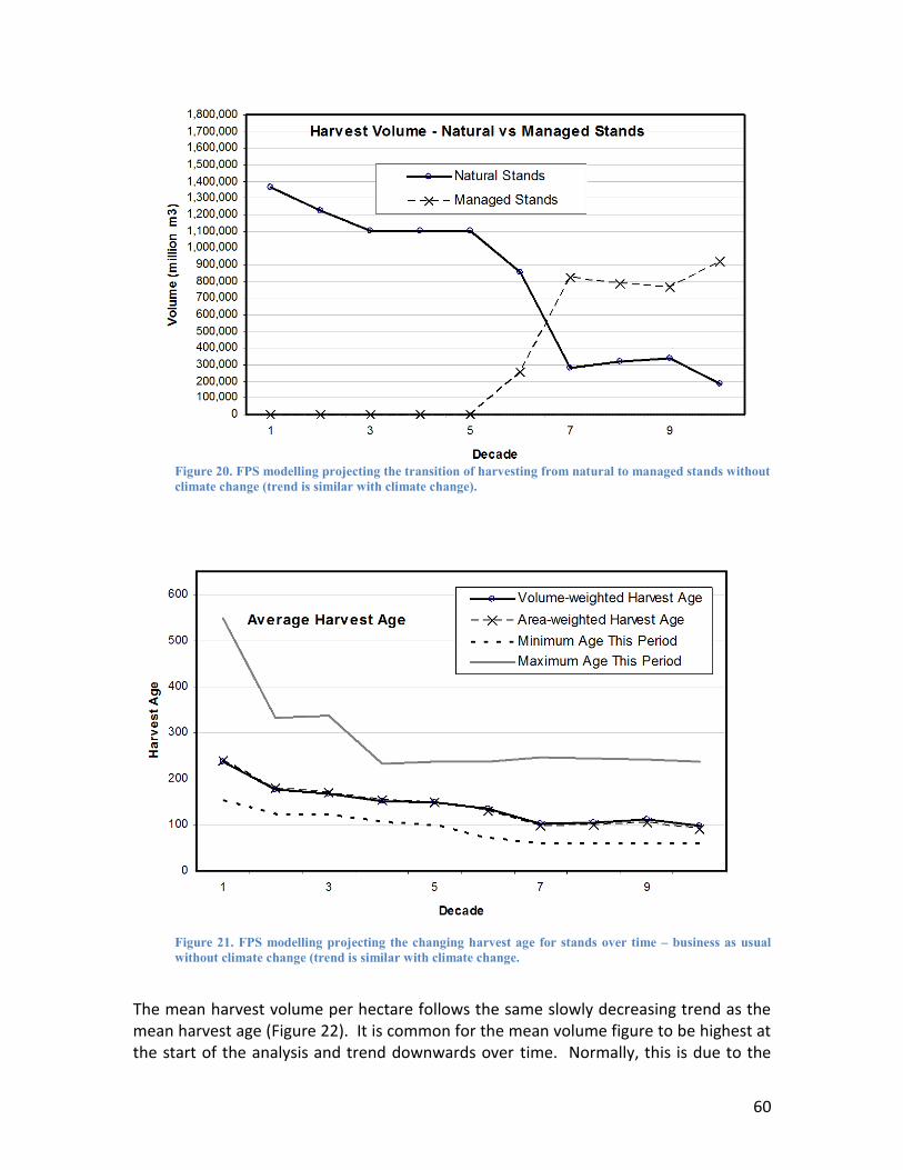
60
Figure 20. FPS modelling projecting the transition of harvesting from natural to managed stands without climate change (trend is similar with climate change).
Figure 21. FPS modelling projecting the changing harvest age for stands over time – business as usual without climate change (trend is similar with climate change.
The mean harvest volume per hectare follows the same slowly decreasing trend as the mean harvest age (Figure 22). It is common for the mean volume figure to be highest at the start of the analysis and trend downwards over time. Normally, this is due to the
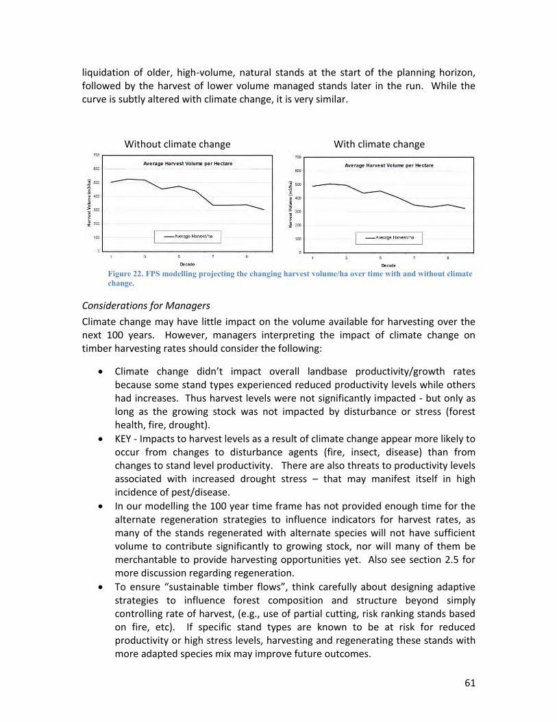
61
liquidation of older, high-volume, natural stands at the start of the planning horizon, followed by the harvest of lower volume managed stands later in the run. While the curve is subtly altered with climate change, it is very similar.
Without climate change With climate change
Figure 22. FPS modelling projecting the changing harvest volume/ha over time with and without climate change.
Considerations for Managers
Climate change may have little impact on the volume available for harvesting over the next 100 years. However, managers interpreting the impact of climate change on timber harvesting rates should consider the following:
Climate change didn’t impact overall landbase productivity/growth rates because some stand types experienced reduced productivity levels while others had increases. Thus harvest levels were not significantly impacted - but only as long as the growing stock was not impacted by disturbance or stress (forest health, fire, drought).
KEY - Impacts to harvest levels as a result of climate change appear more likely to occur from changes to disturbance agents (fire, insect, disease) than from changes to stand level productivity. There are also threats to productivity levels associated with increased drought stress – that may manifest itself in high incidence of pest/disease.
In our modelling the 100 year time frame has not provided enough time for the alternate regeneration strategies to influence indicators for harvest rates, as many of the stands regenerated with alternate species will not have sufficient volume to contribute significantly to growing stock, nor will many of them be merchantable to provide harvesting opportunities yet. Also see section 2.5 for more discussion regarding regeneration.
To ensure “sustainable timber flows”, think carefully about designing adaptive strategies to influence forest composition and structure beyond simply controlling rate of harvest, (e.g., use of partial cutting, risk ranking stands based on fire, etc). If specific stand types are known to be at risk for reduced productivity or high stress levels, harvesting and regenerating these stands with more adapted species mix may improve future outcomes.
62
Mortality due to moisture stress and other species-specific influences (insects and disease)
As previously mentioned, in addition to mortality induced within stands due to inter-tree competition over time, a stand-level mortality algorithm was built into FORECAST Climate as a function of severe moisture stress. When a given moisture stress value exceeded a threshold in a given year and stand unit combination, a species-specific mortality rate was imposed as uniform dispersed mortality throughout the stand. Mortality data from insects and disease within the Kamloops Region were used to refine this mortality factor for lodgepole pine and Douglas-fir.
Considerations for Managers
While our modelling included some uniform partial mortality as a result of moisture stress working in combination with insects and disease, managers should consider the following:
K2 did not consider the impact of climate change and changing host susceptibility on local insect populations to model episodic stand-replacing localized epidemics over time.
K2 also did not consider the possible desychronization of local plant phenological cycles and phases with late spring or early fall frost events (as an example).
If repeated many times due to a changing climate, these factors may show a higher impact on mortality than anticipated in our modelling. This fact should be considered by managers as they consider vulnerabilities and risks over time.
Regeneration
As indicated in the TACA research outcomes, our modelling showed that most tree species have a lower probability of regenerating and establishing as climate change progresses, especially in the second and third climate periods (beyond 2035), where regeneration success is reduced for various species in various ecozones. By the third climate period (> 2065) none of the species in any ecozone is regenerating as well as it is currently.
When considering these results in the dry ecozones (Dry Douglas-fir/ponderosa pine, Dry Lodgepole pine dominated, and the Dry Transition) it should be remembered that TACA assumes regeneration is in an open clearcut condition, similar to the weather station locations that were used to downscale the climate data. It is reasonable to assume that as regeneration success becomes significantly impacted by the changing climate (perhaps in period 2), astute managers would be switching to some type of partial-cutting system for regeneration in all of these types. At the present time, this is already the recommended approach in the Dry Douglas-fir/ ponderosa pine. As our sensitivity analysis of species growing in an understory suggested, regeneration success will be more successful under such a scenario.
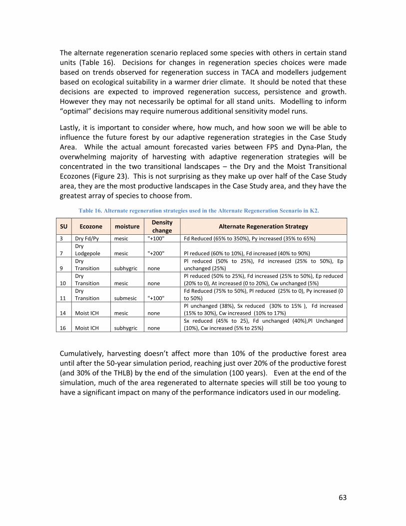
63
The alternate regeneration scenario replaced some species with others in certain stand units (Table 16). Decisions for changes in regeneration species choices were made based on trends observed for regeneration success in TACA and modellers judgement based on ecological suitability in a warmer drier climate. It should be noted that these decisions are expected to improved regeneration success, persistence and growth. However they may not necessarily be optimal for all stand units. Modelling to inform “optimal” decisions may require numerous additional sensitivity model runs.
Lastly, it is important to consider where, how much, and how soon we will be able to influence the future forest by our adaptive regeneration strategies in the Case Study Area. While the actual amount forecasted varies between FPS and Dyna-Plan, the overwhelming majority of harvesting with adaptive regeneration strategies will be concentrated in the two transitional landscapes – the Dry and the Moist Transitional Ecozones (Figure 23). This is not surprising as they make up over half of the Case Study area, they are the most productive landscapes in the Case Study area, and they have the greatest array of species to choose from.
Table 16. Alternate regeneration strategies used in the Alternate Regeneration Scenario in K2.
SU Ecozone moisture Density change
Alternate Regeneration Strategy
3 Dry Fd/Py mesic "+100" Fd Reduced (65% to 350%), Py increased (35% to 65%)
7 Dry Lodgepole mesic "+200" Pl reduced (60% to 10%), Fd increased (40% to 90%)
9 Dry Transition subhygric none
Pl reduced (50% to 25%), Fd increased (25% to 50%), Ep unchanged (25%)
10 Dry Transition mesic none
Pl reduced (50% to 25%), Fd increased (25% to 50%), Ep reduced (20% to 0), At increased (0 to 20%), Cw unchanged (5%)
11 Dry Transition submesic "+100"
Fd Reduced (75% to 50%), Pl reduced (25% to 0), Py increased (0 to 50%)
14 Moist ICH mesic none Pl unchanged (38%), Sx reduced (30% to 15% ), Fd increased (15% to 30%), Cw increased (10% to 17%)
16 Moist ICH subhygric none Sx reduced (45% to 25), Fd unchanged (40%),Pl Unchanged (10%), Cw increased (5% to 25%)
Cumulatively, harvesting doesn’t affect more than 10% of the productive forest area until after the 50-year simulation period, reaching just over 20% of the productive forest (and 30% of the THLB) by the end of the simulation (100 years). Even at the end of the simulation, much of the area regenerated to alternate species will still be too young to have a significant impact on many of the performance indicators used in our modeling.
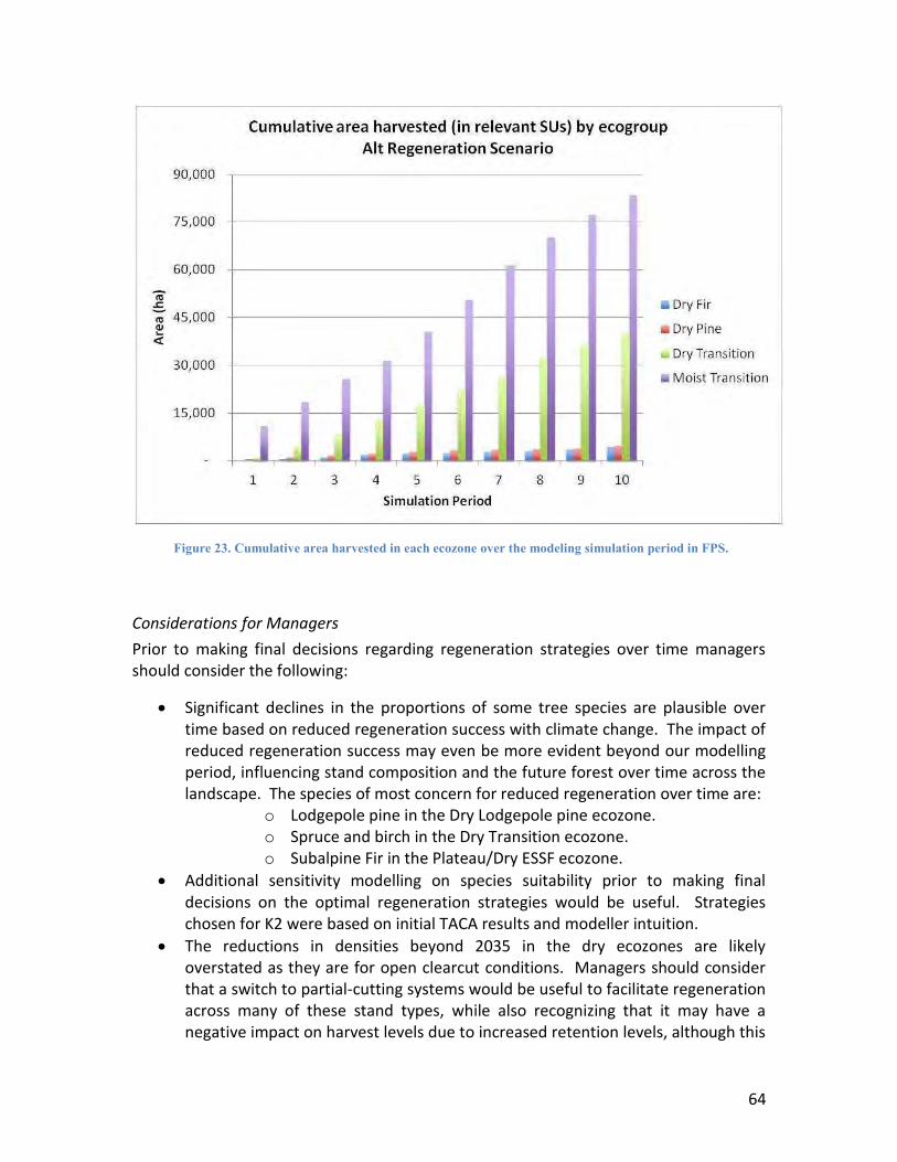
64
Figure 23. Cumulative area harvested in each ecozone over the modeling simulation period in FPS.
Considerations for Managers
Prior to making final decisions regarding regeneration strategies over time managers should consider the following:
Significant declines in the proportions of some tree species are plausible over time based on reduced regeneration success with climate change. The impact of reduced regeneration success may even be more evident beyond our modelling period, influencing stand composition and the future forest over time across the landscape. The species of most concern for reduced regeneration over time are:
o Lodgepole pine in the Dry Lodgepole pine ecozone. o Spruce and birch in the Dry Transition ecozone. o Subalpine Fir in the Plateau/Dry ESSF ecozone.
Additional sensitivity modelling on species suitability prior to making final decisions on the optimal regeneration strategies would be useful. Strategies chosen for K2 were based on initial TACA results and modeller intuition.
The reductions in densities beyond 2035 in the dry ecozones are likely overstated as they are for open clearcut conditions. Managers should consider that a switch to partial-cutting systems would be useful to facilitate regeneration across many of these stand types, while also recognizing that it may have a negative impact on harvest levels due to increased retention levels, although this
65
will depend on the silvicultural system used. Research and careful planning to facilitate this transition should be encouraged.
With reduced regeneration success for broadleaf species, managers should strategically encourage these species in areas that they are projected to decline. Retaining deciduous trees in moister areas of a stand likely would be an appropriate tactic. Careful consideration will be required for management direction regarding brushing and free-growing in those units.
Indicator Trends from Model Results
Trends in the Size of the Timber Harvesting Landbase (THLB)
Unlike the projection in K1, which projected a decrease in the THLB due to because stands that previously provided an economic contribution to harvest flow could no longer do so, K2 modelling projected no reduction in the THLB due to climate change based upon merchantable volume production. This result reflects the growth curves developed in FORECAST for the stand units in the case study area. In most stand units stand productivity actually improved over time. While some units showed declines in productivity with climate change these declines were not great enough to suggest removal from the THLB.
Considerations for Managers
Encourage further research into impacts of climate change on stand level productivity over time. The dendrochronological work linked with the stand level models used in K2 is a good start. As well, simplification of the case study area into 19 stand units may miss impacts on the productive forest landbase at a finer scale. This too deserves further investigation.
Trends in growing stock
Total growing stock (natural and managed) volume declines as a result of the combined effects of harvesting and natural disturbance (Figure 24). This is a trend that is evident even if only the THLB is considered. FPS indicates a slightly larger decline with climate change than under the no climate change scenario, however the important point is that growing stock has not yet reached equilibrium at 100 years and still declines beyond that point.
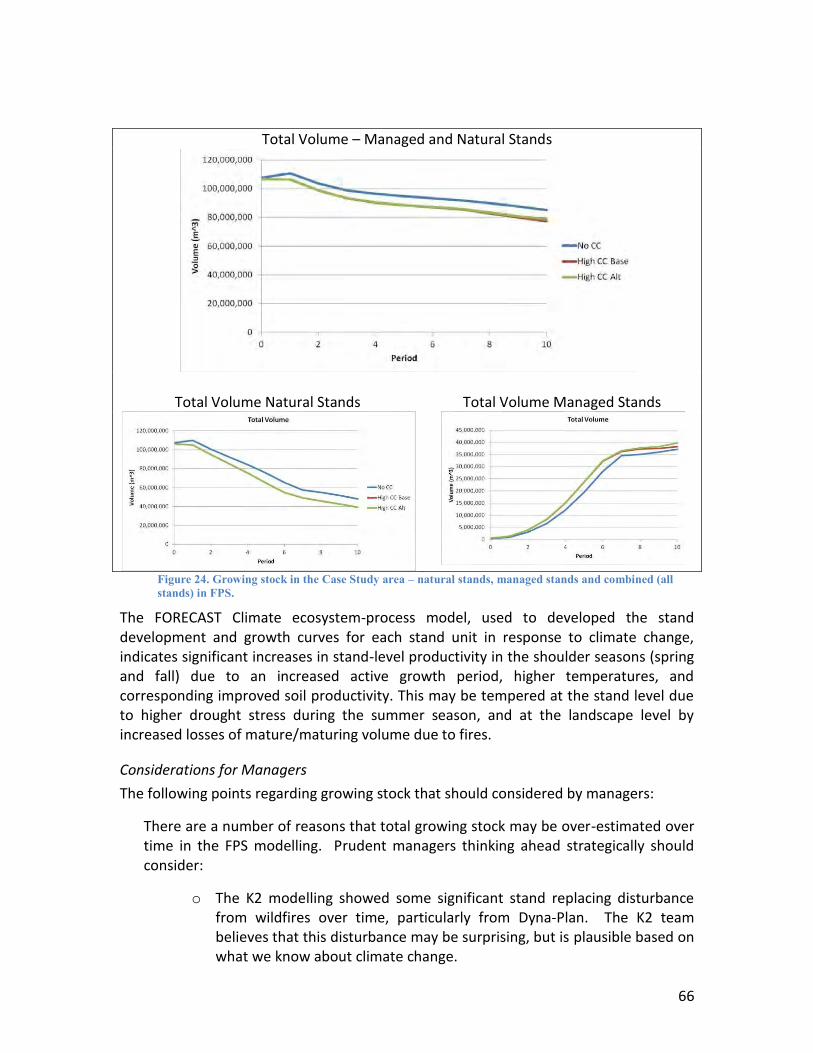
66
Total Volume – Managed and Natural Stands
Total Volume Natural Stands
Total Volume Managed Stands
Figure 24. Growing stock in the Case Study area – natural stands, managed stands and combined (all stands) in FPS.
The FORECAST Climate ecosystem-process model, used to developed the stand development and growth curves for each stand unit in response to climate change, indicates significant increases in stand-level productivity in the shoulder seasons (spring and fall) due to an increased active growth period, higher temperatures, and corresponding improved soil productivity. This may be tempered at the stand level due to higher drought stress during the summer season, and at the landscape level by increased losses of mature/maturing volume due to fires.
Considerations for Managers
The following points regarding growing stock that should considered by managers:
There are a number of reasons that total growing stock may be over-estimated over time in the FPS modelling. Prudent managers thinking ahead strategically should consider:
o The K2 modelling showed some significant stand replacing disturbance from wildfires over time, particularly from Dyna-Plan. The K2 team believes that this disturbance may be surprising, but is plausible based on what we know about climate change.
67
o The K2 modelling is not modelling eruptive surprise events of insect-related mortality where insect populations may explode beyond endemic levels in response to a favourable host as well as favourable conditions for insect population life cycles. Although K2 models included mortality from climate change due to combinations of moisture stress and endemic insects and disease populations interacting with moisture stress, these surprise events could add considerably to this mortality in localized areas during specific climate cycles.
o It is quite possible that climate change may be more severe than the “high climate change” scenario used by K2 suggests.
Trends in leading species
Douglas-fir and lodgepole pine
Douglas-fir leading stands decrease even under the No Climate Change Scenario (NCC), and even more under the High Climate Change Scenario (HCC). The area lost in Douglas-fir leading stands is almost entirely replaced by lodgepole pine leading stands (Figure 25).
Current business-as-usual planting (according to the RESULTS database) is generally favouring pine over Douglas-fir in a number of ecozones for a number of reasons, resulting in general stand-level conversions from Douglas-fir to lodgepole pine even without climate change (Figure 26). This trend is accentuated in the transitional ecozones.
Because stand types in the case study area were simplified to just 19 units, current regeneration strategies from the provincial RESULTS database were averaged across many stands to determine an average strategy. These averages may actually represent few stands on the ground. Leading stand output may not capture what is on the ground, where many areas have been planted mostly to lodgepole pine, or mostly to Douglas-fir. Such a simplification is a necessary part of the modelling process. It must be considered however when reviewing results.
A spatial representation of the case study area with Dyna-Plan shows a similar situation across the case study area, with most of the conversions from Douglas-fir to lodgepole pine occurring throughout the transitional ecozones (Figure 27).
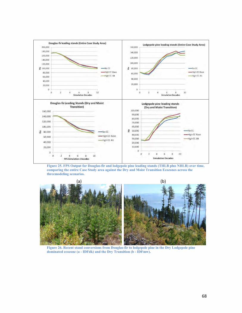
68
Figure 25. FPS Output for Douglas-fir and lodgepole pine leading stands (THLB plus NHLB) over time, comparing the entire Case Study area against the Dry and Moist Transition Ecozones across the threemodeling scenarios.
(a) (b)
Figure 26. Recent stand conversions from Douglas-fir to lodgepole pine in the Dry Lodgepole pine dominated ecozone (a - IDFdk) and the Dry Transition (b - IDFmw).
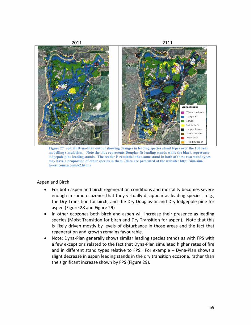
69
2011 2111
Figure 27. Spatial Dyna-Plan output showing changes in leading species stand types over the 100 year modelling simulation. Note the blue represents Douglas-fir leading stands while the black represents lodgepole pine leading stands. The reader is reminded that some stand in both of these two stand types may have a proportion of other species in them. (data are presented at the website: http://sim-sim-forest.comxa.com/k2.html)
Aspen and Birch
For both aspen and birch regeneration conditions and mortality becomes severe enough in some ecozones that they virtually disappear as leading species - e.g., the Dry Transition for birch, and the Dry Douglas-fir and Dry lodgepole pine for aspen (Figure 28 and Figure 29)
In other ecozones both birch and aspen will increase their presence as leading species (Moist Transition for birch and Dry Transition for aspen). Note that this is likely driven mostly by levels of disturbance in those areas and the fact that regeneration and growth remains favourable.
Note: Dyna-Plan generally shows similar leading species trends as with FPS with a few exceptions related to the fact that Dyna-Plan simulated higher rates of fire and in different stand types relative to FPS. For example – Dyna-Plan shows a slight decrease in aspen leading stands in the dry transition ecozone, rather than the significant increase shown by FPS (Figure 29).
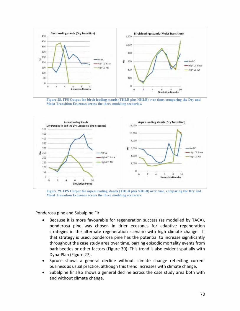
70
Figure 28. FPS Output for birch leading stands (THLB plus NHLB) over time, comparing the Dry and Moist Transition Ecozones across the three modeling scenarios.
Figure 29. FPS Output for aspen leading stands (THLB plus NHLB) over time, comparing the Dry and Moist Transition Ecozones across the three modeling scenarios.
Ponderosa pine and Subalpine Fir
Because it is more favourable for regeneration success (as modelled by TACA), ponderosa pine was chosen in drier ecozones for adaptive regeneration strategies in the alternate regeneration scenario with high climate change. If that strategy is used, ponderosa pine has the potential to increase significantly throughout the case study area over time, barring episodic mortality events from bark beetles or other factors (Figure 30). This trend is also evident spatially with Dyna-Plan (Figure 27).
Spruce shows a general decline without climate change reflecting current business as usual practice, although this trend increases with climate change.
Subalpine fir also shows a general decline across the case study area both with and without climate change.
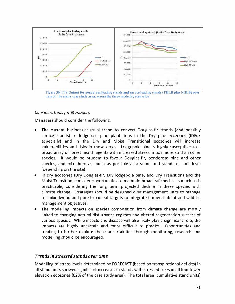
71
Figure 30. FPS Output for ponderosa leading stands and spruce leading stands (THLB plus NHLB) over time on the entire case study area, across the three modeling scenarios.
Considerations for Managers
Managers should consider the following:
The current business-as-usual trend to convert Douglas-fir stands (and possibly spruce stands) to lodgepole pine plantations in the Dry pine ecozones (IDFdk especially) and in the Dry and Moist Transitional ecozones will increase vulnerabilities and risks in those areas. Lodgepole pine is highly susceptible to a broad array of forest health agents with increased stress, much more so than other species. It would be prudent to favour Douglas-fir, ponderosa pine and other species, and mix them as much as possible at a stand and standards unit level (depending on the site).
In dry ecozones (Dry Douglas-fir, Dry lodgepole pine, and Dry Transition) and the Moist Transition, consider opportunities to maintain broadleaf species as much as is practicable, considering the long term projected decline in these species with climate change. Strategies should be designed over management units to manage for mixedwood and pure broadleaf targets to integrate timber, habitat and wildfire management objectives.
The modelling impacts on species composition from climate change are mostly linked to changing natural disturbance regimes and altered regeneration success of various species. While insects and disease will also likely play a significant role, the impacts are highly uncertain and more difficult to predict. Opportunities and funding to further explore these uncertainties through monitoring, research and modelling should be encouraged.
Trends in stressed stands over time
Modelling of stress levels determined by FORECAST (based on transpirational deficits) in all stand units showed significant increases in stands with stressed trees in all four lower elevation ecozones (62% of the case study area). The total area (cumulative stand units)
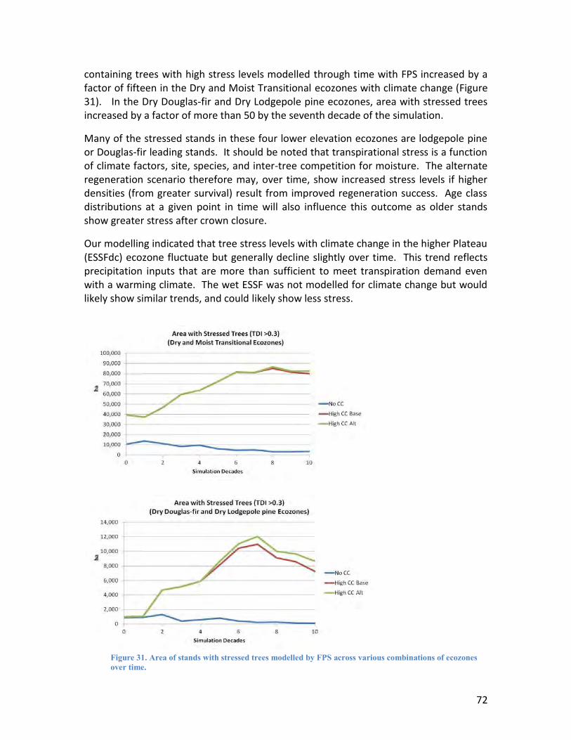
72
containing trees with high stress levels modelled through time with FPS increased by a factor of fifteen in the Dry and Moist Transitional ecozones with climate change (Figure 31). In the Dry Douglas-fir and Dry Lodgepole pine ecozones, area with stressed trees increased by a factor of more than 50 by the seventh decade of the simulation.
Many of the stressed stands in these four lower elevation ecozones are lodgepole pine or Douglas-fir leading stands. It should be noted that transpirational stress is a function of climate factors, site, species, and inter-tree competition for moisture. The alternate regeneration scenario therefore may, over time, show increased stress levels if higher densities (from greater survival) result from improved regeneration success. Age class distributions at a given point in time will also influence this outcome as older stands show greater stress after crown closure.
Our modelling indicated that tree stress levels with climate change in the higher Plateau (ESSFdc) ecozone fluctuate but generally decline slightly over time. This trend reflects precipitation inputs that are more than sufficient to meet transpiration demand even with a warming climate. The wet ESSF was not modelled for climate change but would likely show similar trends, and could likely show less stress.
Figure 31. Area of stands with stressed trees modelled by FPS across various combinations of ecozones over time.
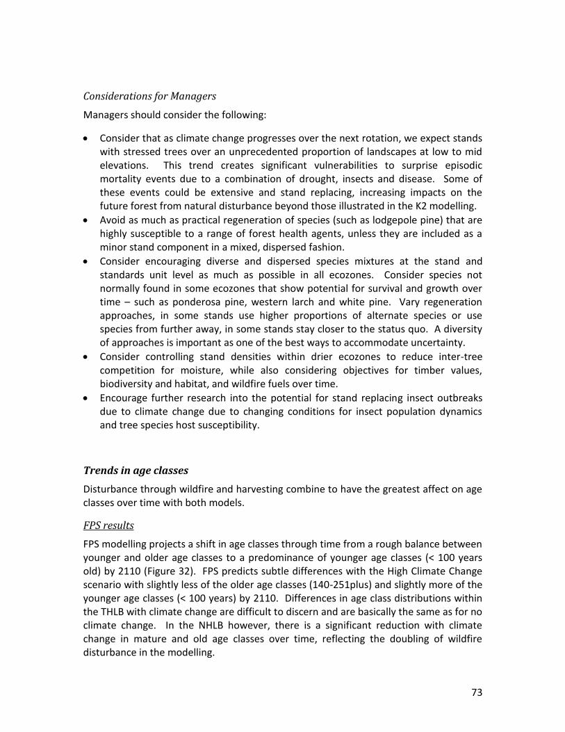
73
Considerations for Managers
Managers should consider the following:
Consider that as climate change progresses over the next rotation, we expect stands with stressed trees over an unprecedented proportion of landscapes at low to mid elevations. This trend creates significant vulnerabilities to surprise episodic mortality events due to a combination of drought, insects and disease. Some of these events could be extensive and stand replacing, increasing impacts on the future forest from natural disturbance beyond those illustrated in the K2 modelling.
Avoid as much as practical regeneration of species (such as lodgepole pine) that are highly susceptible to a range of forest health agents, unless they are included as a minor stand component in a mixed, dispersed fashion.
Consider encouraging diverse and dispersed species mixtures at the stand and standards unit level as much as possible in all ecozones. Consider species not normally found in some ecozones that show potential for survival and growth over time – such as ponderosa pine, western larch and white pine. Vary regeneration approaches, in some stands use higher proportions of alternate species or use species from further away, in some stands stay closer to the status quo. A diversity of approaches is important as one of the best ways to accommodate uncertainty.
Consider controlling stand densities within drier ecozones to reduce inter-tree competition for moisture, while also considering objectives for timber values, biodiversity and habitat, and wildfire fuels over time.
Encourage further research into the potential for stand replacing insect outbreaks due to climate change due to changing conditions for insect population dynamics and tree species host susceptibility.
Trends in age classes
Disturbance through wildfire and harvesting combine to have the greatest affect on age classes over time with both models.
FPS results
FPS modelling projects a shift in age classes through time from a rough balance between younger and older age classes to a predominance of younger age classes (< 100 years old) by 2110 (Figure 32). FPS predicts subtle differences with the High Climate Change scenario with slightly less of the older age classes (140-251plus) and slightly more of the younger age classes (< 100 years) by 2110. Differences in age class distributions within the THLB with climate change are difficult to discern and are basically the same as for no climate change. In the NHLB however, there is a significant reduction with climate change in mature and old age classes over time, reflecting the doubling of wildfire disturbance in the modelling.
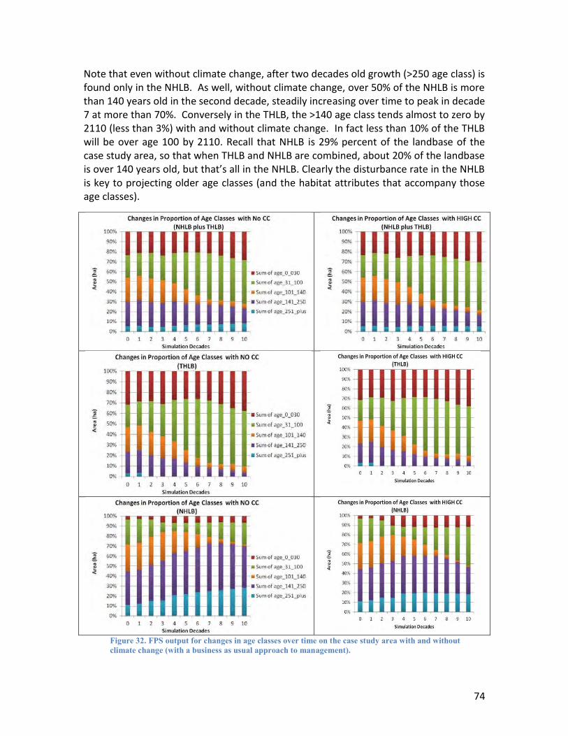
74
Note that even without climate change, after two decades old growth (>250 age class) is found only in the NHLB. As well, without climate change, over 50% of the NHLB is more than 140 years old in the second decade, steadily increasing over time to peak in decade 7 at more than 70%. Conversely in the THLB, the >140 age class tends almost to zero by 2110 (less than 3%) with and without climate change. In fact less than 10% of the THLB will be over age 100 by 2110. Recall that NHLB is 29% percent of the landbase of the case study area, so that when THLB and NHLB are combined, about 20% of the landbase is over 140 years old, but that’s all in the NHLB. Clearly the disturbance rate in the NHLB is key to projecting older age classes (and the habitat attributes that accompany those age classes).
Figure 32. FPS output for changes in age classes over time on the case study area with and without climate change (with a business as usual approach to management).
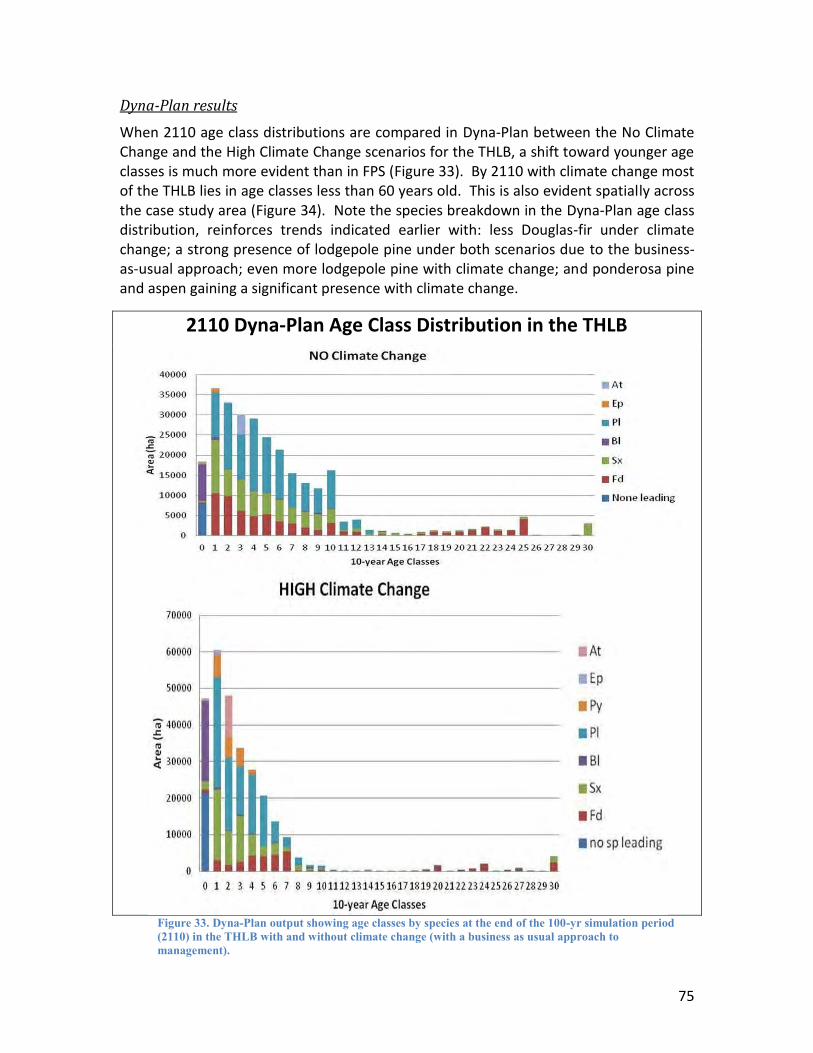
75
Dyna-Plan results
When 2110 age class distributions are compared in Dyna-Plan between the No Climate Change and the High Climate Change scenarios for the THLB, a shift toward younger age classes is much more evident than in FPS (Figure 33). By 2110 with climate change most of the THLB lies in age classes less than 60 years old. This is also evident spatially across the case study area (Figure 34). Note the species breakdown in the Dyna-Plan age class distribution, reinforces trends indicated earlier with: less Douglas-fir under climate change; a strong presence of lodgepole pine under both scenarios due to the business-as-usual approach; even more lodgepole pine with climate change; and ponderosa pine and aspen gaining a significant presence with climate change.
2110 Dyna-Plan Age Class Distribution in the THLB
Figure 33. Dyna-Plan output showing age classes by species at the end of the 100-yr simulation period (2110) in the THLB with and without climate change (with a business as usual approach to management).
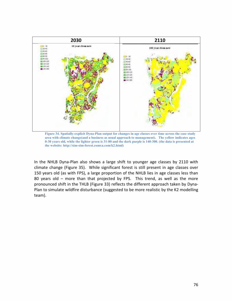
76
2030 2110
Figure 34. Spatially-explicit Dyna-Plan output for changes in age classes over time across the case study area with climate change(and a business as usual approach to management). The yellow indicates ages 0-30 years old, while the lighter green is 31-80 and the dark purple is 140-300. (the data is presented at the website: http://sim-sim-forest.comxa.com/k2.html)
In the NHLB Dyna-Plan also shows a large shift to younger age classes by 2110 with climate change (Figure 35). While significant forest is still present in age classes over 150 years old (as with FPS), a large proportion of the NHLB lies in age classes less than 80 years old – more than that projected by FPS. This trend, as well as the more pronounced shift in the THLB (Figure 33) reflects the different approach taken by Dyna-Plan to simulate wildfire disturbance (suggested to be more realistic by the K2 modelling team).
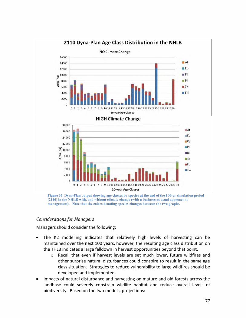
77
2110 Dyna-Plan Age Class Distribution in the NHLB
Figure 35. Dyna-Plan output showing age classes by species at the end of the 100-yr simulation period (2110) in the NHLB with, and without climate change (with a business as usual approach to management). Note that the colors denoting species changes between the two graphs.
Considerations for Managers
Managers should consider the following:
The K2 modelling indicates that relatively high levels of harvesting can be maintained over the next 100 years, however, the resulting age class distribution on the THLB indicates a large falldown in harvest opportunities beyond that point.
o Recall that even if harvest levels are set much lower, future wildfires and other surprise natural disturbances could conspire to result in the same age class situation. Strategies to reduce vulnerability to large wildfires should be developed and implemented.
Impacts of natural disturbance and harvesting on mature and old forests across the landbase could severely constrain wildlife habitat and reduce overall levels of biodiversity. Based on the two models, projections:
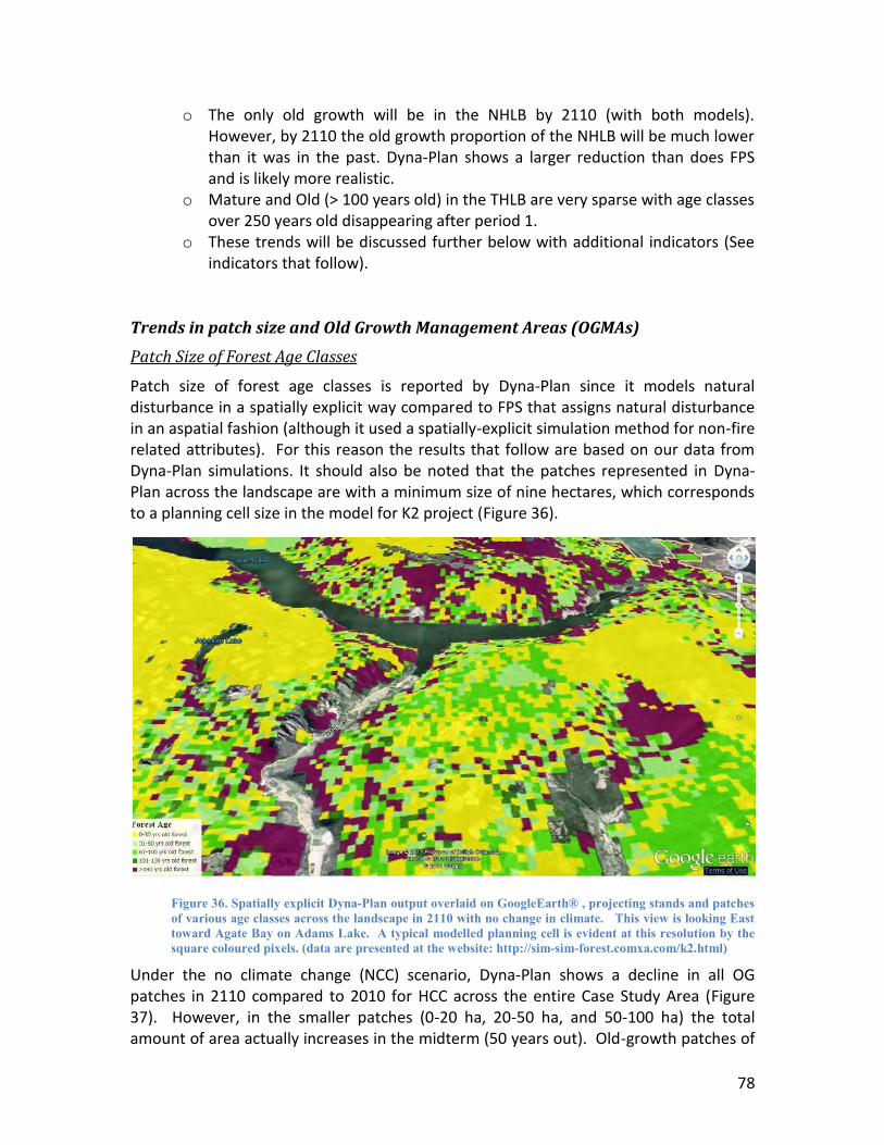
78
o The only old growth will be in the NHLB by 2110 (with both models). However, by 2110 the old growth proportion of the NHLB will be much lower than it was in the past. Dyna-Plan shows a larger reduction than does FPS and is likely more realistic.
o Mature and Old (> 100 years old) in the THLB are very sparse with age classes over 250 years old disappearing after period 1.
o These trends will be discussed further below with additional indicators (See indicators that follow).
Trends in patch size and Old Growth Management Areas (OGMAs)
Patch Size of Forest Age Classes
Patch size of forest age classes is reported by Dyna-Plan since it models natural disturbance in a spatially explicit way compared to FPS that assigns natural disturbance in an aspatial fashion (although it used a spatially-explicit simulation method for non-fire related attributes). For this reason the results that follow are based on our data from Dyna-Plan simulations. It should also be noted that the patches represented in Dyna-Plan across the landscape are with a minimum size of nine hectares, which corresponds to a planning cell size in the model for K2 project (Figure 36).
Figure 36. Spatially explicit Dyna-Plan output overlaid on GoogleEarth® , projecting stands and patches of various age classes across the landscape in 2110 with no change in climate. This view is looking East toward Agate Bay on Adams Lake. A typical modelled planning cell is evident at this resolution by the square coloured pixels. (data are presented at the website: http://sim-sim-forest.comxa.com/k2.html)
Under the no climate change (NCC) scenario, Dyna-Plan shows a decline in all OG patches in 2110 compared to 2010 for HCC across the entire Case Study Area (Figure 37). However, in the smaller patches (0-20 ha, 20-50 ha, and 50-100 ha) the total amount of area actually increases in the midterm (50 years out). Old-growth patches of
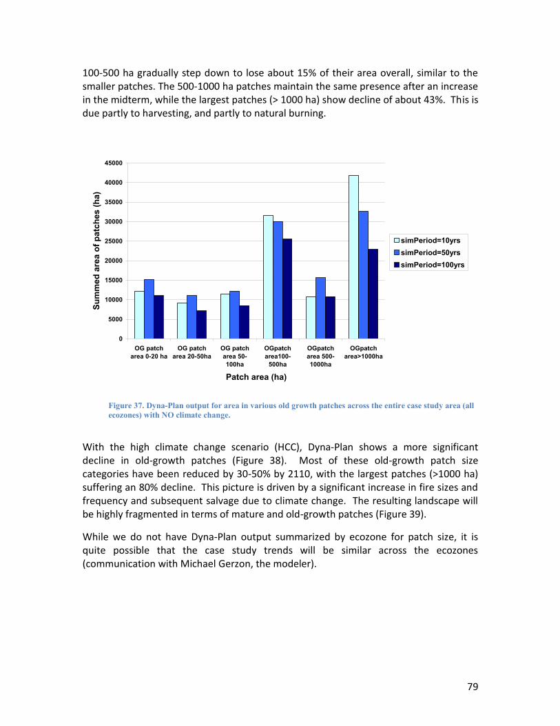
79
100-500 ha gradually step down to lose about 15% of their area overall, similar to the smaller patches. The 500-1000 ha patches maintain the same presence after an increase in the midterm, while the largest patches (> 1000 ha) show decline of about 43%. This is due partly to harvesting, and partly to natural burning.
Figure 37. Dyna-Plan output for area in various old growth patches across the entire case study area (all ecozones) with NO climate change.
With the high climate change scenario (HCC), Dyna-Plan shows a more significant decline in old-growth patches (Figure 38). Most of these old-growth patch size categories have been reduced by 30-50% by 2110, with the largest patches (>1000 ha) suffering an 80% decline. This picture is driven by a significant increase in fire sizes and frequency and subsequent salvage due to climate change. The resulting landscape will be highly fragmented in terms of mature and old-growth patches (Figure 39).
While we do not have Dyna-Plan output summarized by ecozone for patch size, it is quite possible that the case study trends will be similar across the ecozones (communication with Michael Gerzon, the modeler).
0
5000
10000
15000
20000
25000
30000
35000
40000
45000
OG patcharea 0-20 ha
OG patcharea 20-50ha
OG patcharea 50-100ha
OGpatcharea100-
500ha
OGpatcharea 500-1000ha
OGpatcharea>1000ha
Patch area (ha)
Sum
med
are
a of
pat
ches
(ha)
simPeriod=10yrssimPeriod=50yrssimPeriod=100yrs
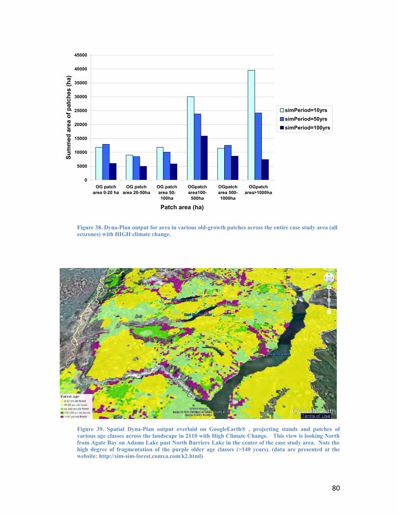
80
Figure 38. Dyna-Plan output for area in various old-growth patches across the entire case study area (all ecozones) with HIGH climate change.
Figure 39. Spatial Dyna-Plan output overlaid on GoogleEarth® , projecting stands and patches of various age classes across the landscape in 2110 with High Climate Change. This view is looking North from Agate Bay on Adams Lake past North Barriere Lake in the center of the case study area. Note the high degree of fragmentation of the purple older age classes (>140 years). (data are presented at the website: http://sim-sim-forest.comxa.com/k2.html)
0
5000
10000
15000
20000
25000
30000
35000
40000
45000
OG patcharea 0-20 ha
OG patcharea 20-50ha
OG patcharea 50-100ha
OGpatcharea100-
500ha
OGpatcharea 500-1000ha
OGpatcharea>1000ha
Patch area (ha)
Sum
med
are
a of
pat
ches
(ha)
simPeriod=10yrssimPeriod=50yrssimPeriod=100yrs
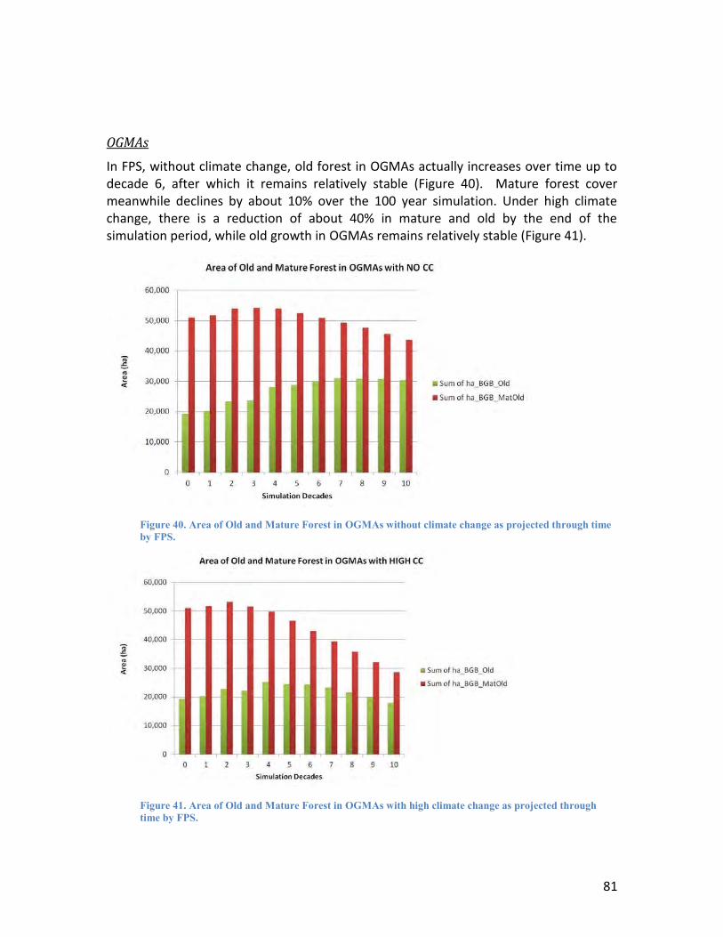
81
OGMAs
In FPS, without climate change, old forest in OGMAs actually increases over time up to decade 6, after which it remains relatively stable (Figure 40). Mature forest cover meanwhile declines by about 10% over the 100 year simulation. Under high climate change, there is a reduction of about 40% in mature and old by the end of the simulation period, while old growth in OGMAs remains relatively stable (Figure 41).
Figure 40. Area of Old and Mature Forest in OGMAs without climate change as projected through time by FPS.
Figure 41. Area of Old and Mature Forest in OGMAs with high climate change as projected through time by FPS.
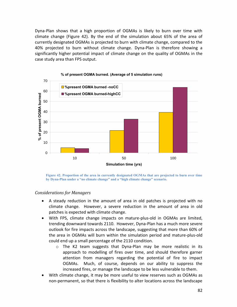
82
Dyna-Plan shows that a high proportion of OGMAs is likely to burn over time with climate change (Figure 42). By the end of the simulation about 65% of the area of currently designated OGMAs is projected to burn with climate change, compared to the 40% projected to burn without climate change. Dyna-Plan is therefore showing a significantly higher potential impact of climate change on the quality of OGMAs in the case study area than FPS output.
Figure 42. Proportion of the area in currently designated OGMAs that are projected to burn over time by Dyna-Plan under a “no climate change” and a “high climate change” scenario.
Considerations for Managers
A steady reduction in the amount of area in old patches is projected with no climate change. However, a severe reduction in the amount of area in old patches is expected with climate change.
With FPS, climate change impacts on mature-plus-old in OGMAs are limited, trending downward towards 2110. However, Dyna-Plan has a much more severe outlook for fire impacts across the landscape, suggesting that more than 60% of the area in OGMAs will burn within the simulation period and mature-plus-old could end up a small percentage of the 2110 condition.
o The K2 team suggests that Dyna-Plan may be more realistic in its approach to modelling of fires over time, and should therefore garner attention from managers regarding the potential of fire to impact OGMAs. Much, of course, depends on our ability to suppress the increased fires, or manage the landscape to be less vulnerable to them.
With climate change, it may be more useful to view reserves such as OGMAs as non-permanent, so that there is flexibility to alter locations across the landscape
0
10
20
30
40
50
60
70
10 50 100
Simulation time (yrs)
% o
f pre
sent
OG
MA
bur
ned
%present OGMA burned -noCC
%present OGMA burned-highCC
% of present OGMA burned. (Average of 5 simulation runs)
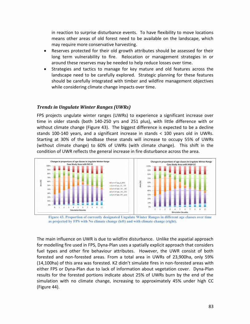
83
in reaction to surprise disturbance events. To have flexibility to move locations means other areas of old forest need to be available on the landscape, which may require more conservative harvesting.
Reserves protected for their old growth attributes should be assessed for their long term vulnerability to fire. Relocation or management strategies in or around these reserves may be needed to help reduce losses over time.
Strategies and tactics to manage for key mature and old features across the landscape need to be carefully explored. Strategic planning for these features should be carefully integrated with timber and wildfire management objectives while considering climate change impacts over time.
Trends in Ungulate Winter Ranges (UWRs)
FPS projects ungulate winter ranges (UWRs) to experience a significant increase over time in older stands (both 140-250 yrs and 251 plus), with little difference with or without climate change (Figure 43). The biggest difference is expected to be a decline stands 100-140 years, and a significant increase in stands < 100 years old in UWRs. Starting at 30% of the landbase these stands will increase to occupy 55% of UWRs (without climate change) to 60% of UWRs (with climate change). This shift in the condition of UWR reflects the general increase in fire disturbance across the area.
Figure 43. Proportion of currently designated Ungulate Winter Ranges in different age classes over time as projected by FPS with No climate change (left) and with climate change (right).
The main influence on UWR is due to wildfire disturbance. Unlike the aspatial approach for modelling fire used in FPS, Dyna-Plan uses a spatially explicit approach that considers fuel types and other fire behaviour attributes. However, the UWR consist of both forested and non-forested areas. From a total area in UWRs of 23,900ha, only 59% (14,100ha) of this area was forested. K2 didn’t simulate fires in non-forested areas with either FPS or Dyna-Plan due to lack of information about vegetation cover. Dyna-Plan results for the forested portions indicate about 25% of UWRs burn by the end of the simulation with no climate change, increasing to approximately 45% under high CC (Figure 44).
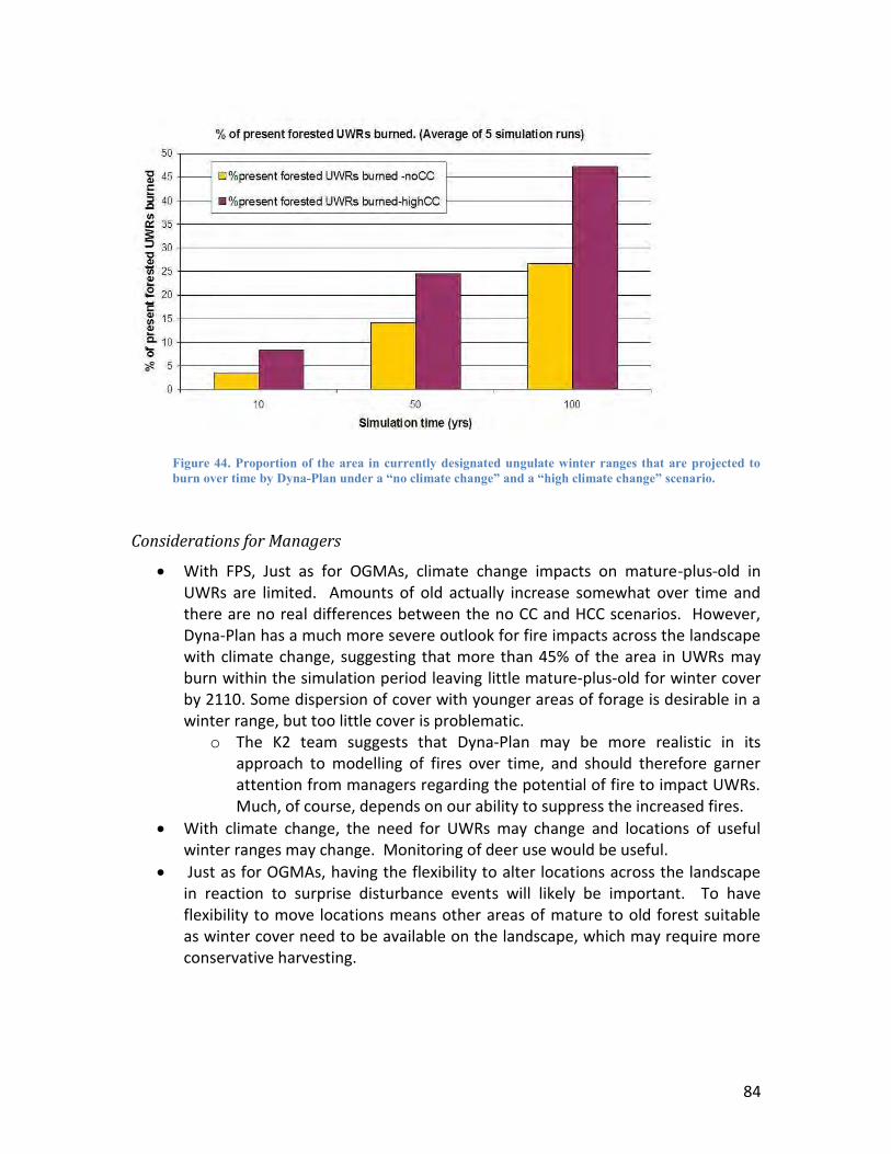
84
Figure 44. Proportion of the area in currently designated ungulate winter ranges that are projected to burn over time by Dyna-Plan under a “no climate change” and a “high climate change” scenario.
Considerations for Managers
With FPS, Just as for OGMAs, climate change impacts on mature-plus-old in UWRs are limited. Amounts of old actually increase somewhat over time and there are no real differences between the no CC and HCC scenarios. However, Dyna-Plan has a much more severe outlook for fire impacts across the landscape with climate change, suggesting that more than 45% of the area in UWRs may burn within the simulation period leaving little mature-plus-old for winter cover by 2110. Some dispersion of cover with younger areas of forage is desirable in a winter range, but too little cover is problematic.
o The K2 team suggests that Dyna-Plan may be more realistic in its approach to modelling of fires over time, and should therefore garner attention from managers regarding the potential of fire to impact UWRs. Much, of course, depends on our ability to suppress the increased fires.
With climate change, the need for UWRs may change and locations of useful winter ranges may change. Monitoring of deer use would be useful.
Just as for OGMAs, having the flexibility to alter locations across the landscape in reaction to surprise disturbance events will likely be important. To have flexibility to move locations means other areas of mature to old forest suitable as winter cover need to be available on the landscape, which may require more conservative harvesting.
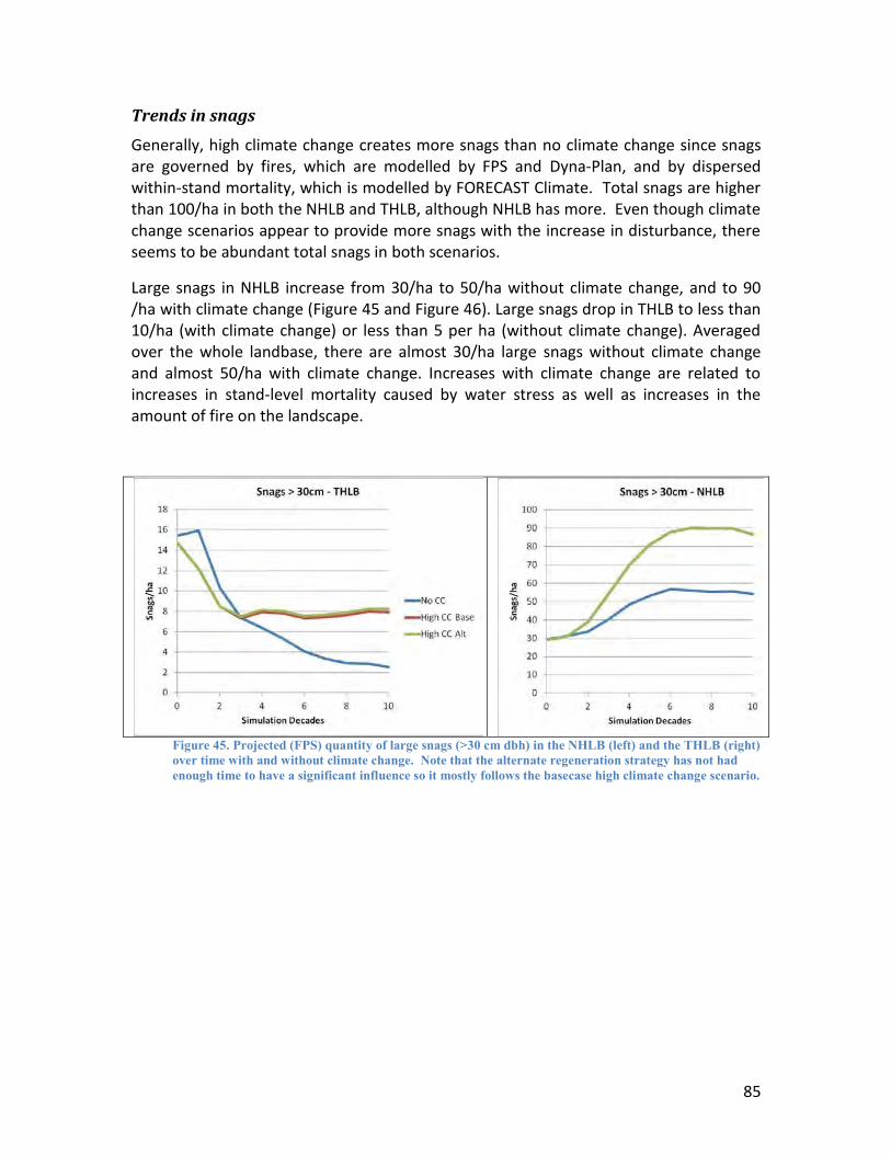
85
Trends in snags
Generally, high climate change creates more snags than no climate change since snags are governed by fires, which are modelled by FPS and Dyna-Plan, and by dispersed within-stand mortality, which is modelled by FORECAST Climate. Total snags are higher than 100/ha in both the NHLB and THLB, although NHLB has more. Even though climate change scenarios appear to provide more snags with the increase in disturbance, there seems to be abundant total snags in both scenarios.
Large snags in NHLB increase from 30/ha to 50/ha without climate change, and to 90 /ha with climate change (Figure 45 and Figure 46). Large snags drop in THLB to less than 10/ha (with climate change) or less than 5 per ha (without climate change). Averaged over the whole landbase, there are almost 30/ha large snags without climate change and almost 50/ha with climate change. Increases with climate change are related to increases in stand-level mortality caused by water stress as well as increases in the amount of fire on the landscape.
Figure 45. Projected (FPS) quantity of large snags (>30 cm dbh) in the NHLB (left) and the THLB (right) over time with and without climate change. Note that the alternate regeneration strategy has not had enough time to have a significant influence so it mostly follows the basecase high climate change scenario.
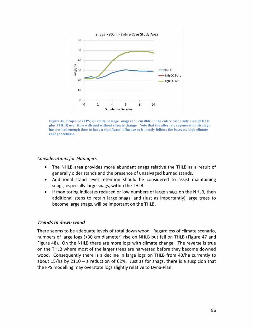
86
Figure 46. Projected (FPS) quantity of large snags (>30 cm dbh) in the entire case study area (NHLB plus THLB) over time with and without climate change. Note that the alternate regeneration strategy has not had enough time to have a significant influence so it mostly follows the basecase high climate change scenario.
Considerations for Managers
The NHLB area provides more abundant snags relative the THLB as a result of generally older stands and the presence of unsalvaged burned stands.
Additional stand level retention should be considered to assist maintaining snags, especially large snags, within the THLB.
If monitoring indicates reduced or low numbers of large snags on the NHLB, then additional steps to retain large snags, and (just as importantly) large trees to become large snags, will be important on the THLB.
Trends in down wood
There seems to be adequate levels of total down wood. Regardless of climate scenario, numbers of large logs (>30 cm diameter) rise on NHLB but fall on THLB (Figure 47 and Figure 48). On the NHLB there are more logs with climate change. The reverse is true on the THLB where most of the larger trees are harvested before they become downed wood. Consequently there is a decline in large logs on THLB from 40/ha currently to about 15/ha by 2110 – a reduction of 62%. Just as for snags, there is a suspicion that the FPS modelling may overstate logs slightly relative to Dyna-Plan.
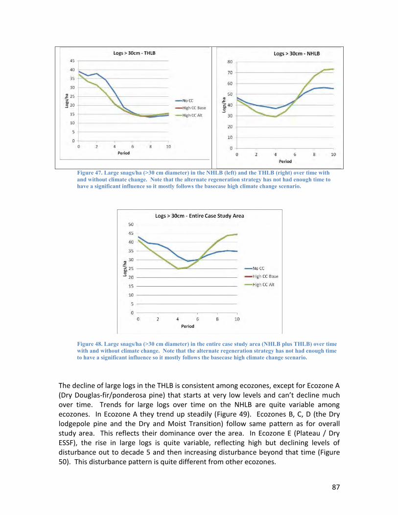
87
Figure 47. Large snags/ha (>30 cm diameter) in the NHLB (left) and the THLB (right) over time with and without climate change. Note that the alternate regeneration strategy has not had enough time to have a significant influence so it mostly follows the basecase high climate change scenario.
Figure 48. Large snags/ha (>30 cm diameter) in the entire case study area (NHLB plus THLB) over time with and without climate change. Note that the alternate regeneration strategy has not had enough time to have a significant influence so it mostly follows the basecase high climate change scenario.
The decline of large logs in the THLB is consistent among ecozones, except for Ecozone A (Dry Douglas-fir/ponderosa pine) that starts at very low levels and can’t decline much over time. Trends for large logs over time on the NHLB are quite variable among ecozones. In Ecozone A they trend up steadily (Figure 49). Ecozones B, C, D (the Dry lodgepole pine and the Dry and Moist Transition) follow same pattern as for overall study area. This reflects their dominance over the area. In Ecozone E (Plateau / Dry ESSF), the rise in large logs is quite variable, reflecting high but declining levels of disturbance out to decade 5 and then increasing disturbance beyond that time (Figure 50). This disturbance pattern is quite different from other ecozones.
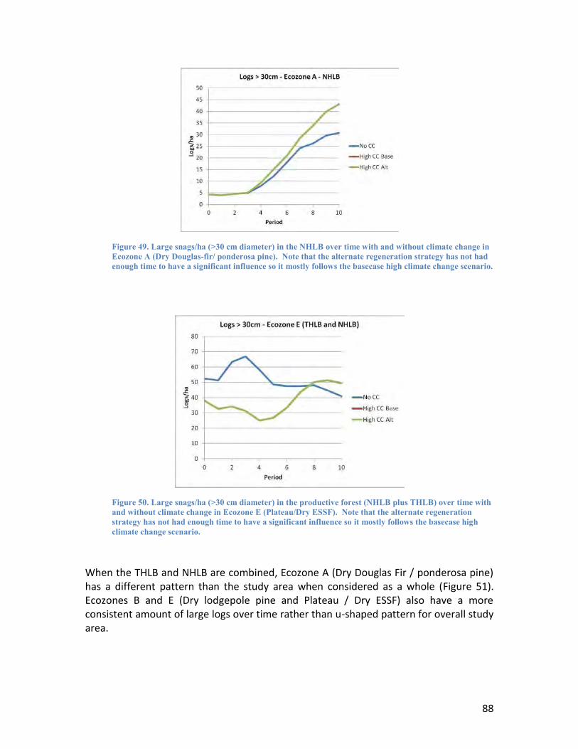
88
Figure 49. Large snags/ha (>30 cm diameter) in the NHLB over time with and without climate change in Ecozone A (Dry Douglas-fir/ ponderosa pine). Note that the alternate regeneration strategy has not had enough time to have a significant influence so it mostly follows the basecase high climate change scenario.
Figure 50. Large snags/ha (>30 cm diameter) in the productive forest (NHLB plus THLB) over time with and without climate change in Ecozone E (Plateau/Dry ESSF). Note that the alternate regeneration strategy has not had enough time to have a significant influence so it mostly follows the basecase high climate change scenario.
When the THLB and NHLB are combined, Ecozone A (Dry Douglas Fir / ponderosa pine) has a different pattern than the study area when considered as a whole (Figure 51). Ecozones B and E (Dry lodgepole pine and Plateau / Dry ESSF) also have a more consistent amount of large logs over time rather than u-shaped pattern for overall study area.
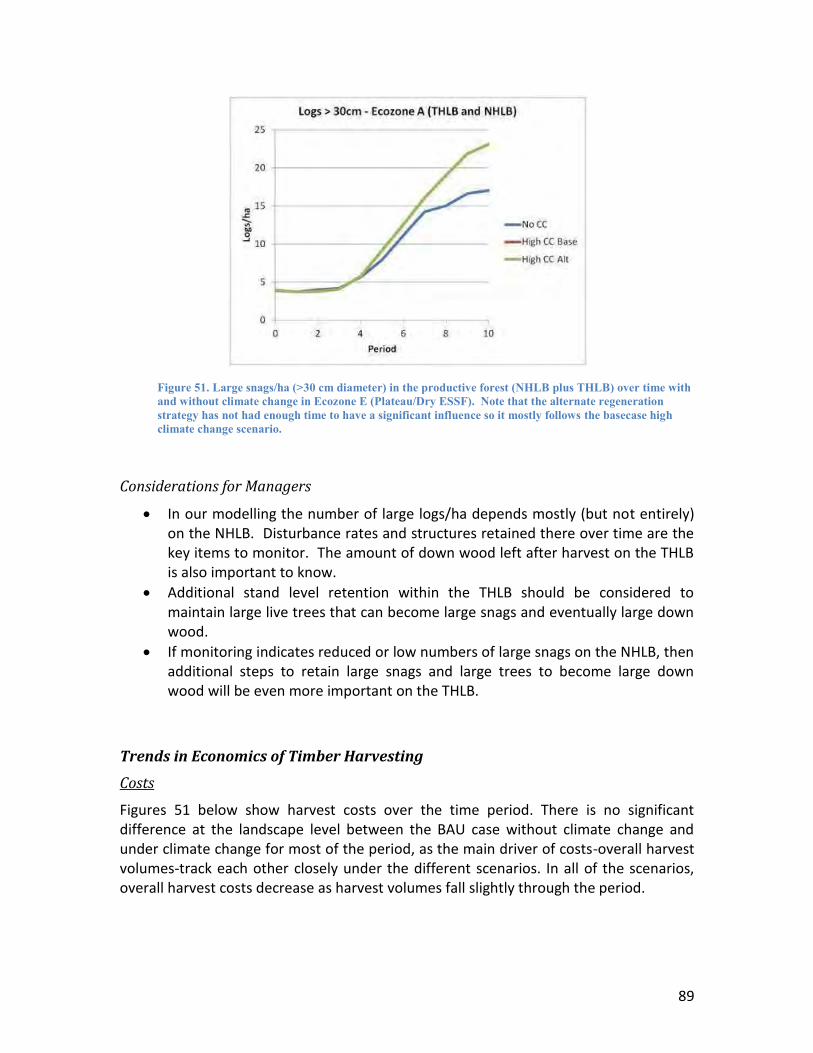
89
Figure 51. Large snags/ha (>30 cm diameter) in the productive forest (NHLB plus THLB) over time with and without climate change in Ecozone E (Plateau/Dry ESSF). Note that the alternate regeneration strategy has not had enough time to have a significant influence so it mostly follows the basecase high climate change scenario.
Considerations for Managers
In our modelling the number of large logs/ha depends mostly (but not entirely) on the NHLB. Disturbance rates and structures retained there over time are the key items to monitor. The amount of down wood left after harvest on the THLB is also important to know.
Additional stand level retention within the THLB should be considered to maintain large live trees that can become large snags and eventually large down wood.
If monitoring indicates reduced or low numbers of large snags on the NHLB, then additional steps to retain large snags and large trees to become large down wood will be even more important on the THLB.
Trends in Economics of Timber Harvesting
Costs
Figures 51 below show harvest costs over the time period. There is no significant difference at the landscape level between the BAU case without climate change and under climate change for most of the period, as the main driver of costs-overall harvest volumes-track each other closely under the different scenarios. In all of the scenarios, overall harvest costs decrease as harvest volumes fall slightly through the period.
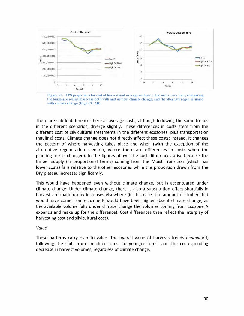
90
Figure 51. FPS projections for cost of harvest and average cost per cubic metre over time, comparing the business-as-usual basecase both with and without climate change, and the alternate regen scenario with climate change (High CC Alt).
There are subtle differences here as average costs, although following the same trends in the different scenarios, diverge slightly. These differences in costs stem from the different cost of silvicultural treatments in the different ecozones, plus transportation (hauling) costs. Climate change does not directly affect these costs; instead, it changes the pattern of where harvesting takes place and when (with the exception of the alternative regeneration scenario, where there are differences in costs when the planting mix is changed). In the figures above, the cost differences arise because the timber supply (in proportional terms) coming from the Moist Transition (which has lower costs) falls relative to the other ecozones while the proportion drawn from the Dry plateau increases significantly.
This would have happened even without climate change, but is accentuated under climate change. Under climate change, there is also a substitution effect-shortfalls in harvest are made up by increases elsewhere (in this case, the amount of timber that would have come from ecozone B would have been higher absent climate change, as the available volume falls under climate change the volumes coming from Ecozone A expands and make up for the difference). Cost differences then reflect the interplay of harvesting cost and silvicultural costs.
Value
These patterns carry over to value. The overall value of harvests trends downward, following the shift from an older forest to younger forest and the corresponding decrease in harvest volumes, regardless of climate change.
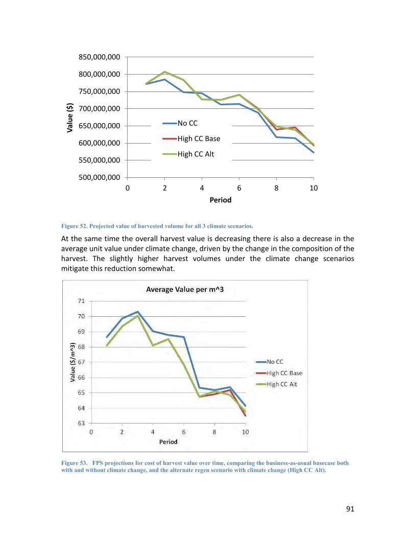
91
Figure 52. Projected value of harvested volume for all 3 climate scenarios.
At the same time the overall harvest value is decreasing there is also a decrease in the average unit value under climate change, driven by the change in the composition of the harvest. The slightly higher harvest volumes under the climate change scenarios mitigate this reduction somewhat.
Figure 53. FPS projections for cost of harvest value over time, comparing the business-as-usual basecase both with and without climate change, and the alternate regen scenario with climate change (High CC Alt).
500,000,000
550,000,000
600,000,000
650,000,000
700,000,000
750,000,000
800,000,000
850,000,000
0 2 4 6 8 10
Val
ue
($)
Period
No CC
High CC Base
High CC Alt
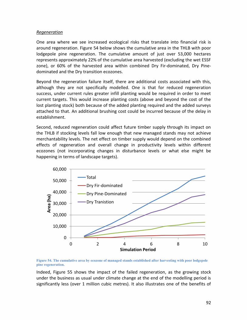
92
Regeneration
One area where we see increased ecological risks that translate into financial risk is around regeneration. Figure 54 below shows the cumulative area in the THLB with poor lodgepole pine regeneration. The cumulative amount of just over 53,000 hectares represents approximately 22% of the cumulative area harvested (excluding the wet ESSF zone), or 60% of the harvested area within combined Dry Fir-dominated, Dry Pine-dominated and the Dry transition ecozones.
Beyond the regeneration failure itself, there are additional costs associated with this, although they are not specifically modelled. One is that for reduced regeneration success, under current rules greater infill planting would be required in order to meet current targets. This would increase planting costs (above and beyond the cost of the lost planting stock) both because of the added planting required and the added surveys attached to that. An additional brushing cost could be incurred because of the delay in establishment.
Second, reduced regeneration could affect future timber supply through its impact on the THLB if stocking levels fall low enough that new managed stands may not achieve merchantability levels. The net effect on timber supply would depend on the combined effects of regeneration and overall change in productivity levels within different ecozones (not incorporating changes in disturbance levels or what else might be happening in terms of landscape targets).
Figure 54. The cumulative area by ecozone of managed stands established after harvesting with poor lodgepole pine regeneration.
Indeed, Figure 55 shows the impact of the failed regeneration, as the growing stock under the business as usual under climate change at the end of the modelling period is significantly less (over 1 million cubic metres). It also illustrates one of the benefits of
0
10,000
20,000
30,000
40,000
50,000
60,000
0 2 4 6 8 10
Are
a (h
a)
Simulation Period
Total
Dry Fir-dominated
Dry Pine-Dominated
Dry Tranistion
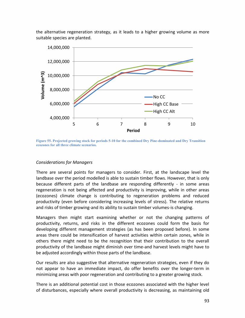
93
the alternative regeneration strategy, as it leads to a higher growing volume as more suitable species are planted.
Figure 55. Projected growing stock for periods 5-10 for the combined Dry Pine-dominated and Dry Transition ecozones for all three climate scenarios.
Considerations for Managers
There are several points for managers to consider. First, at the landscape level the landbase over the period modelled is able to sustain timber flows. However, that is only because different parts of the landbase are responding differently - in some areas regeneration is not being affected and productivity is improving, while in other areas (ecozones) climate change is contributing to regeneration problems and reduced productivity (even before considering increasing levels of stress). The relative returns and risks of timber growing-and its ability to sustain timber volumes-is changing.
Managers then might start examining whether or not the changing patterns of productivity, returns, and risks in the different ecozones could form the basis for developing different management strategies (as has been proposed before). In some areas there could be intensification of harvest activities within certain zones, while in others there might need to be the recognition that their contribution to the overall productivity of the landbase might diminish over time-and harvest levels might have to be adjusted accordingly within those parts of the landbase.
Our results are also suggestive that alternative regeneration strategies, even if they do not appear to have an immediate impact, do offer benefits over the longer-term in minimizing areas with poor regeneration and contributing to a greater growing stock.
There is an additional potential cost in those ecozones associated with the higher level of disturbances, especially where overall productivity is decreasing, as maintaining old
4,000,000
6,000,000
8,000,000
10,000,000
12,000,000
14,000,000
5 6 7 8 9 10
Vo
lum
e (m
^3)
Period
No CC
High CC Base
High CC Alt
94
growth requires reserving more timber to offset the expected losses-but that further reduces the amount of timber available for harvest.
We did not model or explore the costs associated with holding timber stock, but we also note there is an increased risk in carrying an older forest under climate change as the longer you wait to harvest there is an increased chance you will lose it from the increased disturbance levels. This is again a trade-off managers may want to explore, not only in how they are managing the landscape but also in evaluating rotation ages for different types of stands.
We also did not explore the timing for those stands that are suffering the effects of climate change-and if there might be an optimal time to enter/convert a stand that might otherwise become unmerchantable or where the planting window might vanish. This is again an area amenable to exploration within the modelling framework we have developed.
95
Collaboration and Communication
Community Outreach
The K2 research team spent time both in Clearwater and Barriere, British Columbia to share the initial findings of the K2 project, and to hear observations about climate change from residents. Public presentations and discussions were held over the course of several days with over 100 participants of all ages and affiliations, including:
The BC Ministry of Forests and Range
BC Timber Sales
Clearwater Community Forest
Woodlot licensees
Junior Council of high school students
Tourism Wells Gray
Official Community Plan Steering Committee and District Council
Clearwater Ski Hill Society and Wells Gray Outdoors Club
Community members from Barriere, including the Mayor and a Councillor
Presentations compared key findings from the initial K1 project with local observations on the ground. Discussions highlighted that communities’ knowledge of possible impacts from climate change is growing, and that a number of the project’s findings (primarily from K1) for forests do in fact reflect what people in Clearwater are seeing.
We found that people are already thinking about climate change adaptation (Appendix A13 Cleawater Outreach report 05-06-09.doc). In Clearwater, for example, groups are considering how best to include issues of climate change in the tourism sector, such as the impacts of less snow at lower elevations. In addition, the Official Clearwater Community Plan will examine flood and wildfire risks. The K2 project team remains available to support community adaptation and is always eager to share findings from the K2 project and analyse them alongside the ongoing observations of community members.
Client Meetings and Input
K2 was a client-based multi-disciplinary process of exploration and learning, designed to link researchers, agency and licensee managers, local communities and other stakeholders in an adaptive management fashion. A process such as K2, therefore, requires an engaged and supportive locally based group to champion and guide its development (i.e. the clients). In K2, the team of clients consisted of representatives from:
the Kamloops Timber Supply Area major licensees,
the local Ministry of Forests, Lands, and Natural Resource Operations (formerly the Ministry of Forests and Range); and
the local Ministry of Environment
96
The purpose of assembling the clients was to:
1. Ensure the project is relevant locally. 2. Develop a common understanding of:
a. the project itself and its objectives b. terminology and concepts utilized in the project; c. the forest models, their assumptions, capabilities, utility, and integration; d. climate scenarios, their assumptions and purpose.
3. Manage expectations of what the models and project can actually deliver. 4. Build buy-in, critical for implementation of project outcomes.
Communication, participation and engagement have been the foundation of the Kamloops Future Forest Strategy (both K1 and K2) with interaction occurring at multiple levels (Figure 5256). K2 integrated K1 assumptions into a learning approach that utilized the modelling framework to engage participants. Meetings and workshops have ensured project relevance locally, steered the modelling process, provided transparency, and helped build relationships, essential for moving forward with identified adaptive actions.
Outreach sessions with local government and community groups in the Kamloops TSA have also been important for project input and local planning. This format for the exploration of climate change will help further our knowledge and understanding, but the process is cyclical and continuous. Next steps include implementing management recommendations, monitoring, analysis, and asking more questions.
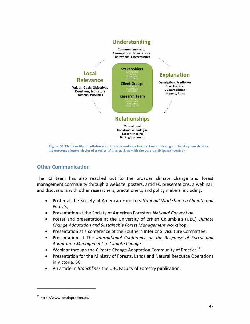
97
Figure 52 The benefits of collaboration in the Kamloops Future Forest Strategy. The diagram depicts the outcomes (outer circle) of a series of interactions with the core participants (centre).
Other Communication
The K2 team has also reached out to the broader climate change and forest management community through a website, posters, articles, presentations, a webinar, and discussions with other researchers, practitioners, and policy makers, including:
Poster at the Society of American Foresters National Workshop on Climate and Forests,
Presentation at the Society of American Foresters National Convention,
Poster and presentation at the University of British Columbia’s (UBC) Climate Change Adaptation and Sustainable Forest Management workshop,
Presentation at a conference of the Southern Interior Silviculture Committee,
Presentation at The International Conference on the Response of Forest and Adaptation Management to Climate Change
Webinar through the Climate Change Adaptation Community of Practice11
Presentation for the Ministry of Forests, Lands and Natural Resource Operations in Victoria, BC.
An article in Branchlines the UBC Faculty of Forestry publication.
11 http://www.ccadaptation.ca/
98
Conclusions The purpose of this chapter is threefold.
First, we summarize the broader management implications that flow from our analyses, and how modelling has informed the assessment of risks and options under climate change. We also offer our thoughts on next steps in extending the assessments including more analysis at different scales.
Second, we explore what was learned as we developed the different models used in the analysis, primarily TACA and FORECAST-Climate. Our focus here is on what insight was gained from using process-based models to explore forest regeneration and growth, including a better understanding of how forests might respond to climate change (what we can learn from moving beyond qualitative assessments) and where additional research could help refine our assumptions and improve our understanding of how climate change will affect forest ecosystems.
Finally, we discuss the broader implications from this project, including policy considerations. We also suggest how these models could be used to enhance adaptive capacity, and in particular how this kind of modelling approach could be incorporated into more formalized frameworks. This section is more speculative, as we are still in the process of sharing outputs with managers and practitioners, but we draw on general needs identified in the literature.
Summary of Sensitivities, Risks and Associated Adaptation Suggestions for Management in the Kamloops TSA
General Trends
One of our primary goals for the project had been around understanding the feasibility of different options, likely outcomes if we do not adjust our management outcomes, and how we might affect those outcomes by introducing different management strategies. In the preceding sections we look at following a business-as-usual approach and the consequences under climate change, and then evaluated as an alternative management strategy alternative regeneration in those stands that are displaying regeneration issues. The key trends and primary management concerns are summarized below. While we did not model other management actions, we also offer suggestions based on insights from stand-level modelling and landscape level results on other actions that could reduce risks from the BAU approach.
In the discussion of results that preceded this section, key stand and landscape level performance indicators were used to present and interpret modelling results. Many of the indicators illustrated subtle and sometimes very little impact from climate change. Examples of indicators, which show little change, include growing stock, productivity,
99
average harvest volume per hectare, harvest age, and amount of productive area (size of the timber supply landbase), harvesting costs and timber values. Some indicators such as snags and coarse woody debris actually increase in stands subject to climate change in the non-timber harvesting landbase (but are reduced to very low levels on the THLB and over the study area as a whole). Productivity and most other indicators also seem to generally improve at higher elevations (even in the dry ESSF) where abundant moisture and higher temperature in spring and fall could improve conditions generally.
An important factor to remember when considering the results of this modelling project is the 100-year time horizon. It is widely recognized that beyond 100 years, the uncertainty associated with climate change overwhelms any projections of impacts. However, under the climate scenario chosen, our modelling results show that in this area we are unlikely to detect some key potential impacts from climate change; or to test the ability to mitigate these impacts with adaptive options over a one hundred year time frame.
For example, the modelling showed that timber harvest flows can be maintained over the modelling period at relatively high and constant levels with just a small apparent decline in growing stock. However, the real challenges for timber harvesting flows may be in the next 50-100 years beyond our modelling timeline. From a stand-level perspective, we found that the impacts on productivity are minimal in younger stands and become progressively more pronounced as stands age (older than 80-100 years). Hence, the true risks (and thus the full impact) to ecosystem productivity from current planting prescriptions are likely to be manifested after the time horizon we considered. Similarly, adaptive strategies to plant alternate species appear to have little influence on timber harvesting flow and other indicators mostly because it takes more than 100 years to accumulate enough growing stock in enough stands on the landscape to really make a difference to many of the indicators.
Some of the indicators used in K2 for our business-as-usual approach with climate change decline significantly (relative to preferred levels), sometimes at alarming levels. These will be the focus for the summary of sensitivities, risks and recommendations that follow. You are encouraged to explore the preceding discussion of modelling results for more information. A key feature of these few declining indicators is that they place significant risk on the achievement of management goals established with our clients:
Our goal of maintaining or increasing the flow of timber volume and/or value appears at significant risk beyond 2100 (up to that point it can be met, but will be influenced greatly by salvage).
Our goal of no loss of native species due to management – is also be a risk over time especially for species relying on older forest types. The point is arguable on the basis of whether it is management or nature that is responsible, but none-the-less should garner management attention.
Our goal to minimize risk of fire to people and property is also at significant risk.
100
The overarching goal of encouraging resilience to maintain productive “healthy” forests with continued capacity to provide future benefits (i.e. the essence of sustainability) also appears to be at risk with our business-as-usual approach.
We believe that in spite of the assumptions and uncertainties incorporated into our modelling and detailed in preceding sections of this report that the risks to our management goals are sufficiently serious to warrant adaptations in our management approach. This case study area may be in the Kamloops TSA, but the implications are relevant for much of the Southern Interior in similar ecological landscapes.
Key Ecological Sensitivity and Management Risks
One of the challenges in the original K1 project had been understanding how stand level risks (and management strategies) would translate up at the landscape level, including the consequences of different management strategies. One of the findings from the modelling was that at the landscape level in the K2 study area, differences in stands and how they responded under climate change when averaged across the landscape suggested there would be little change. Yet closer analysis revealed more significant change, especially in some stand units, and a divergence in how different parts of the landscape were responding-where in some cases climate change on the whole had limited effect or was even contributing to improved outcomes, while in other cases it was raising challenges, either around regeneration, productivity, or mortality.
In the discussion below we focus on ecozones as the appropriate analysis unit in our assessment of impacts and risks. There are also the stand level impacts, some of which are consistent within the ecozone (reflecting the adaptation of stands to that particular climactic environment and how they respond to climactic factors), although there are differences in responses.
The results from FORECAST Climate suggest that climate change under the modelled A1B1 scenario will have both positive and negative impacts on stand-level productivity in the K2 project area. The warming of air temperatures generally led to a lengthening of the growing season in all ecozones. In addition, climate warming led to increases in the decomposition of dead organic matter and the associated release of nutrients. Both of these effects had a positive impact on stand-level productivity. In contrast, climate change consistently led to an increase in mid-growing season water stress which had a negative impact on growth rates and often resulted in increased mortality. The net impact of these competing effects on long-term stand productivity depended on a number of factors including: stand age at the time of the climate change simulation, species composition, soil edaphic conditions, and ecozone.
Table 17 below summarizes the key sensitivities, risks and actions as informed by the modelling. In particular, they emphasize that it is in certain parts of the landbase-the drier parts-and with certain species-lodgepole pine –where those sensitivities are concentrated, and the consequences and risks that flow from a business as usual
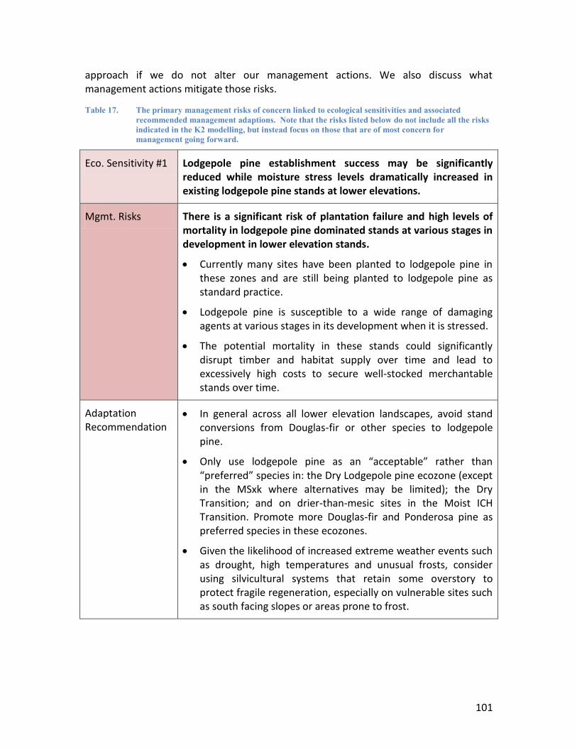
101
approach if we do not alter our management actions. We also discuss what management actions mitigate those risks.
Table 17. The primary management risks of concern linked to ecological sensitivities and associated recommended management adaptions. Note that the risks listed below do not include all the risks indicated in the K2 modelling, but instead focus on those that are of most concern for management going forward.
Eco. Sensitivity #1 Lodgepole pine establishment success may be significantly reduced while moisture stress levels dramatically increased in existing lodgepole pine stands at lower elevations.
Mgmt. Risks There is a significant risk of plantation failure and high levels of mortality in lodgepole pine dominated stands at various stages in development in lower elevation stands.
Currently many sites have been planted to lodgepole pine in these zones and are still being planted to lodgepole pine as standard practice.
Lodgepole pine is susceptible to a wide range of damaging agents at various stages in its development when it is stressed.
The potential mortality in these stands could significantly disrupt timber and habitat supply over time and lead to excessively high costs to secure well-stocked merchantable stands over time.
Adaptation Recommendation
In general across all lower elevation landscapes, avoid stand conversions from Douglas-fir or other species to lodgepole pine.
Only use lodgepole pine as an “acceptable” rather than “preferred” species in: the Dry Lodgepole pine ecozone (except in the MSxk where alternatives may be limited); the Dry Transition; and on drier-than-mesic sites in the Moist ICH Transition. Promote more Douglas-fir and Ponderosa pine as preferred species in these ecozones.
Given the likelihood of increased extreme weather events such as drought, high temperatures and unusual frosts, consider using silvicultural systems that retain some overstory to protect fragile regeneration, especially on vulnerable sites such as south facing slopes or areas prone to frost.
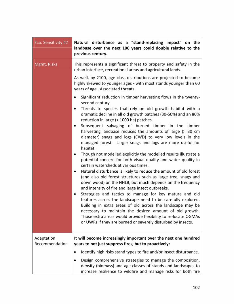
102
Eco. Sensitivity #2 Natural disturbance as a “stand-replacing impact” on the landbase over the next 100 years could double relative to the previous century.
Mgmt. Risks This represents a significant threat to property and safety in the urban interface, recreational areas and agricultural lands.
As well, by 2100, age class distributions are projected to become highly skewed to younger ages - with most stands younger than 60 years of age. Associated threats:
Significant reduction in timber harvesting flows in the twenty-second century.
Threats to species that rely on old growth habitat with a dramatic decline in all old growth patches (30-50%) and an 80% reduction in large (> 1000 ha) patches.
Subsequent salvaging of burned timber in the timber harvesting landbase reduces the amounts of large (> 30 cm diameter) snags and logs (CWD) to very low levels in the managed forest. Larger snags and logs are more useful for habitat.
Though not modelled explicitly the modelled results illustrate a potential concern for both visual quality and water quality in certain watersheds at various times.
Natural disturbance is likely to reduce the amount of old forest (and also old forest structures such as large tree, snags and down wood) on the NHLB, but much depends on the frequency and intensity of fire and large insect outbreaks.
Strategies and tactics to manage for key mature and old features across the landscape need to be carefully explored. Building in extra areas of old across the landscape may be necessary to maintain the desired amount of old growth. Those extra areas would provide flexibility to re-locate OGMAs or UWRs if they are burned or severely disturbed by insects.
Adaptation Recommendation
It will become increasingly important over the next one hundred years to not just suppress fires, but to proactively:
Identify high risks stand types to fire and/or insect disturbance.
Design comprehensive strategies to manage the composition, density (biomass) and age classes of stands and landscapes to increase resilience to wildfire and manage risks for both fire
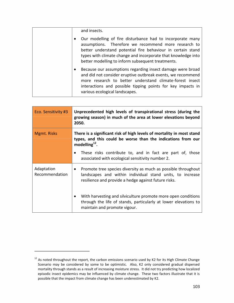
103
and insects.
Our modelling of fire disturbance had to incorporate many assumptions. Therefore we recommend more research to better understand potential fire behaviour in certain stand types with climate change and incorporate that knowledge into better modelling to inform subsequent treatments.
Because our assumptions regarding insect damage were broad and did not consider eruptive outbreak events, we recommend more research to better understand climate-forest insect interactions and possible tipping points for key impacts in various ecological landscapes.
Eco. Sensitivity #3 Unprecedented high levels of transpirational stress (during the growing season) in much of the area at lower elevations beyond 2050.
Mgmt. Risks There is a significant risk of high levels of mortality in most stand types, and this could be worse than the indications from our modelling12.
These risks contribute to, and in fact are part of, those associated with ecological sensitivity number 2.
Adaptation Recommendation
Promote tree species diversity as much as possible throughout landscapes and within individual stand units, to increase resilience and provide a hedge against future risks.
With harvesting and silviculture promote more open conditions through the life of stands, particularly at lower elevations to maintain and promote vigour.
12 As noted throughout the report, the carbon emissions scenario used by K2 for its High Climate Change Scenario may be considered by some to be optimistic. Also, K2 only considered gradual dispersed mortality through stands as a result of increasing moisture stress. It did not try predicting how localized episodic insect epidemics may be influenced by climate change. These two factors illustrate that it is possible that the impact from climate change has been underestimated by K2.
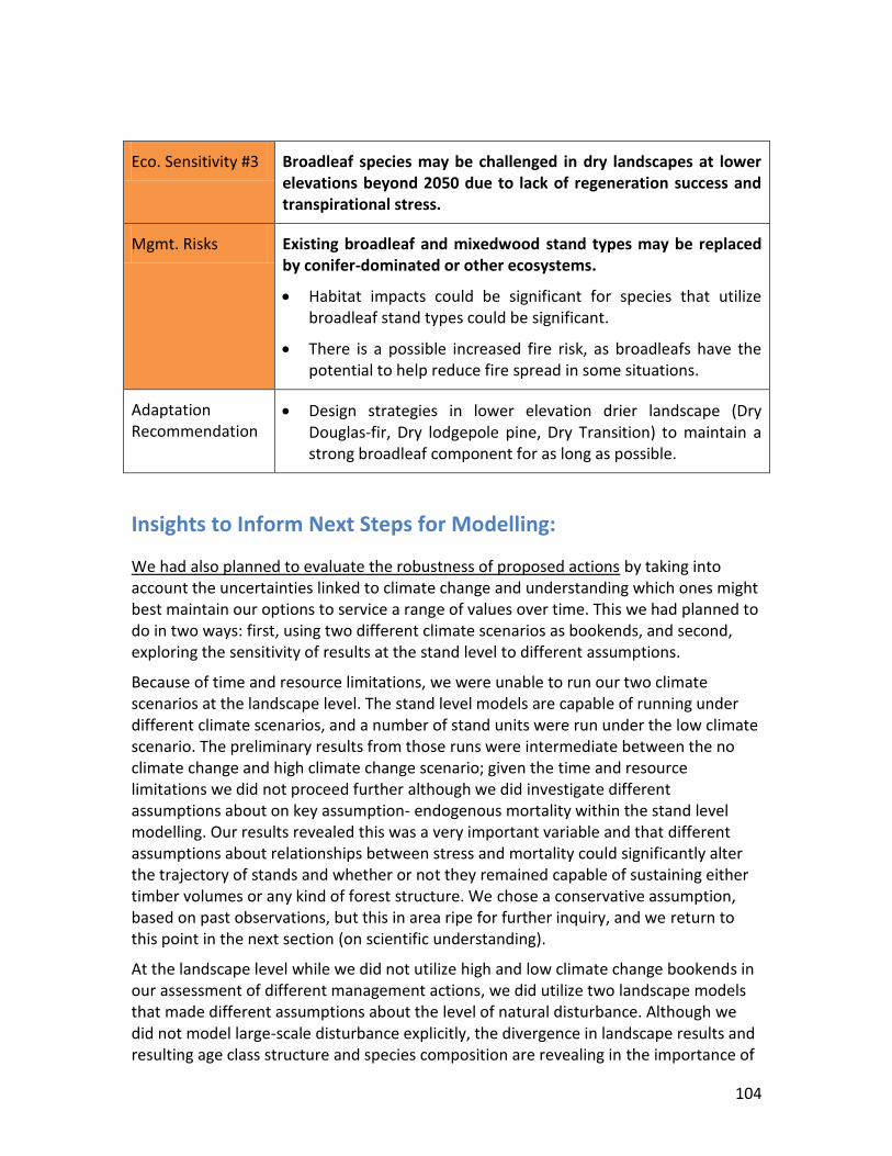
104
Eco. Sensitivity #3 Broadleaf species may be challenged in dry landscapes at lower elevations beyond 2050 due to lack of regeneration success and transpirational stress.
Mgmt. Risks Existing broadleaf and mixedwood stand types may be replaced by conifer-dominated or other ecosystems.
Habitat impacts could be significant for species that utilize broadleaf stand types could be significant.
There is a possible increased fire risk, as broadleafs have the potential to help reduce fire spread in some situations.
Adaptation Recommendation
Design strategies in lower elevation drier landscape (Dry Douglas-fir, Dry lodgepole pine, Dry Transition) to maintain a strong broadleaf component for as long as possible.
Insights to Inform Next Steps for Modelling:
We had also planned to evaluate the robustness of proposed actions by taking into account the uncertainties linked to climate change and understanding which ones might best maintain our options to service a range of values over time. This we had planned to do in two ways: first, using two different climate scenarios as bookends, and second, exploring the sensitivity of results at the stand level to different assumptions.
Because of time and resource limitations, we were unable to run our two climate scenarios at the landscape level. The stand level models are capable of running under different climate scenarios, and a number of stand units were run under the low climate scenario. The preliminary results from those runs were intermediate between the no climate change and high climate change scenario; given the time and resource limitations we did not proceed further although we did investigate different assumptions about on key assumption- endogenous mortality within the stand level modelling. Our results revealed this was a very important variable and that different assumptions about relationships between stress and mortality could significantly alter the trajectory of stands and whether or not they remained capable of sustaining either timber volumes or any kind of forest structure. We chose a conservative assumption, based on past observations, but this in area ripe for further inquiry, and we return to this point in the next section (on scientific understanding).
At the landscape level while we did not utilize high and low climate change bookends in our assessment of different management actions, we did utilize two landscape models that made different assumptions about the level of natural disturbance. Although we did not model large-scale disturbance explicitly, the divergence in landscape results and resulting age class structure and species composition are revealing in the importance of
105
how this might affect achieving management values. We again return to this point in the next section (on scientific understanding).
We did find value in comparing outcomes from different strategies to be useful in identifying the efficacy of different actions. We would expect additional insight by extending the scenarios and consideration of actions, although we do note that there are practical limitations to the number of different combinations that can be explored. However, taking that into account, we do see the value in using this approach to identify “robust strategies” and we also feel that there is value in building an approach that allows managers to “test” strategies, including exploring the sensitivity of the outcomes to different assumptions about how ecosystems might respond. We examine this point in more detail in the final section.
Scientific Insight and Further Research
Another objective we had in this project was to explicitly identify assumptions and knowledge gaps that will require further research and/or monitoring over time. We also anticipated that developing a process-based model would shed insight into how climate change would impact forests that we would be unable to obtain through either envelope-based modelling or qualitative assessments, given the complexity of relationships and interplay between all the different factors influencing forest growth and renewal.
Our modelling confirmed that intuition. The response of a given stand type to climate change is dependent upon its current age. Young stands appear to have more flexibility in their response to climate change in that they have a greater capacity (through stand self-thinning, interspecific competition, etc.) to adapt to changing conditions over an extended period of time. Stress-levels in general also tended to be relatively lower in young stands. In contrast, existing mature stands (e.g. > ~60 years) have developed characteristics that reflect past climate and may be more vulnerable to rapidly changing climates
Our modelling also revealed the importance of site-specific characteristics. Climate change led to dramatic increases in tree water stress in most of the ecozones examined in the Kamloops area. While this stress did not appear to be great enough to lead directly levels of mortality that significantly reduced merchantable yields in most simulated stand units, based on past historical records and simulating past stand development, we did find large areas of the landscape where stress was rising. This pointed to several key knowledge gaps. First, we need to develop a better understanding of the long-term implications of increased moisture stress in stands and whether or not there may be threshold effects (mortality increases significantly when it exceeds a certain point) or whether sequencing may be important (the combination of two or more years of sequential stress events). Second, we need to better understand at the landscape level whether or not the presence of large areas of chronically stressed stands may enhance their vulnerability to biotic disturbance agents.
106
Our modelling showed that increases in temperature during the spring and fall led to enhanced productivity in many stand units, particularly in higher elevation ecozones. More work is needed to evaluate the potential negative impacts of early and late growing season frosts on growth and mortality.
Our model results suggest that interactions between species within stands can influence stand-development patterns under climate change. More work needs to be done to develop our understanding of these interactions. In particular, some stand level modelling results suggest that different silvicultural treatments and planting mixes for stands that are traditionally not considered might be effective ways to reduce risks.
Stress is likely the most important indicator that FORECAST Climate provides for species suitability as it has the ability to identify vulnerability of species with a changing climate. While mortality is difficult if not impossible to predict, levels of stress can be used to gauge risk to reduced growth, and the potential for impacts from insects and disease and hence long term reliability.
Finally, process-based models (in this case FORECAST Climate) provide a powerful and flexible tool for exploring the long-term impacts of climate change on stand growth and development.
Generalizing the K2 Approach-how can it contribute to Adaptive Capacity?
One of our objectives was to translate the K2 process undertaken and the lessons learned for application in similar efforts elsewhere.
We first consider the broader question of using modelling to explore different scenarios and using those results to then informs policy and decision-making, given the uncertainty associated with climate change. We then turn to the equally broad question of how this kind of approach can contribute to adaptive capacity, both in an institutional way, but also in how it can be used to address the increasingly challenging problem of managing complexity in an increasingly uncertain world.
Scarlett (2010) identified a number of major ways in which science can help inform policy. The first was around improving vulnerability assessments, by helping managers prioritize risks, and assisting them in assessing the likely outcome of different actions and how they address those risks. A second way in which they could contribute was to enhancing adaptive management, including exploring how different actions would work across different scales and integrated across different values, and how they might need to be tailored to specific circumstances, including local or regional conditions. Finally, scientists could contribute the development of dashboard indicators-broad performance indicators that would show whether or not we are headed in the right direction.
In our discussion so far we have explored how our modeling has addressed the first point: providing assistance in prioritizing risks and assisting mangers in selecting actions.
At least five areas of management should be addressed given climate change and models-especially when they are linked across different scales can offer insight too managers looking for guidance. First, managers can use harvesting and stand tending
107
techniques that facilitate seedling survival, control competition, and direct successional processes. Second, the topic foremost in the literature, managers can actively match species and genotypes to environments for which they are optimally adapted. Third, effort can be directed at reducing forest susceptibility to insects, disease and fire. Fourth managers can plan stand and landscapes in patterns that either enables species to move or put obstacles in their way. Fifth, forest management policies should change to reflect climate change and models allow mangers to see whether their current policies will necessarily achieve the planned results.
At a practical level while the models underline the massive amount of uncertainty, they can show direction of trends, and scope out possible magnitudes. They can also indicate sites of most sensitivity. For managers and practitioners that need to make decisions, models serve to add credence to our assumptions and gut feelings, which is a very good thing. For example,
a. Models help identify impacts on survival and stress by species instead of
us simply guessing that certain species will be impacted. TACA helps with
‘real, i.e., based on scientifically calculated limiting factors’ projections of
probability of establishment that are based on more data than we can
assimilate in our heads.
b. FORECAST can show us that stress on different species is actually
increasing and in which units it is most pronounced, which is useful even
when we don’t know exactly what it takes for a tree to die or how insects
and disease respond to that stress to have an easier time.
c. FPS and Dyna-plan can show us that static reserves likely will burn –
either a little or a lot, and so strategies for maintaining old forest values
likely will need to change. Primarily, those landscape models are book
keepers showing summaries of TACA and Forecast across landscapes.
Again, that bookkeeping is not trivial, we cannot visualize the future
landscapes without the help of models.
More generally, this model-based approach also addresses another of Scarlett’s points-it can support proactive adaptive management. As shown in Figure 57 below, what models offer is conceptual linkages-hypotheses-linking how management actions will impact outcomes. This then assists in identifying the indicators and how monitoring can be used to adjust management actions-increasingly important where we anticipate that some effects may not manifest themselves for decades, even as we plant trees now that will be exposed to far different climates in the future. It also lets us build on our understanding, and continually improve our models.
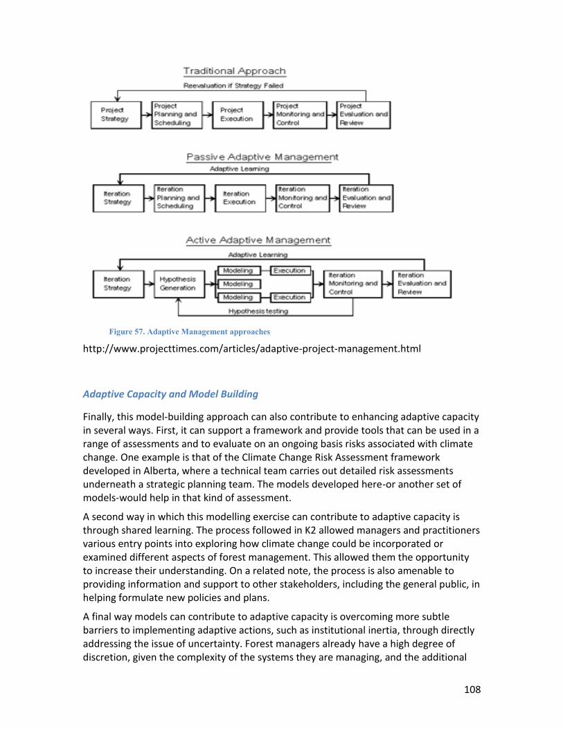
108
Figure 57. Adaptive Management approaches
http://www.projecttimes.com/articles/adaptive-project-management.html
Adaptive Capacity and Model Building
Finally, this model-building approach can also contribute to enhancing adaptive capacity in several ways. First, it can support a framework and provide tools that can be used in a range of assessments and to evaluate on an ongoing basis risks associated with climate change. One example is that of the Climate Change Risk Assessment framework developed in Alberta, where a technical team carries out detailed risk assessments underneath a strategic planning team. The models developed here-or another set of models-would help in that kind of assessment.
A second way in which this modelling exercise can contribute to adaptive capacity is through shared learning. The process followed in K2 allowed managers and practitioners various entry points into exploring how climate change could be incorporated or examined different aspects of forest management. This allowed them the opportunity to increase their understanding. On a related note, the process is also amenable to providing information and support to other stakeholders, including the general public, in helping formulate new policies and plans.
A final way models can contribute to adaptive capacity is overcoming more subtle barriers to implementing adaptive actions, such as institutional inertia, through directly addressing the issue of uncertainty. Forest managers already have a high degree of discretion, given the complexity of the systems they are managing, and the additional
109
complexity introduced by climate change could potentially make it more difficulty to make choices given the emphasis on uncertainty and what could happen. Most management has focused on those things that are more predictable; less discussion has been directed at how to cope with the uncertainty that characterizes most future scenarios. Given the importance of long-term planning in forest management, uncertainty in projections of future growth and yield under changing climates is one of the fundamental challenges that forest managers will have to face in developing adaptation plans and strategies.
A key point is that magnitudes of change are uncertain, but change is certain and the model results allow a good guess at the direction of change and the areas of most change. The models help affirm the large uncertainty in magnitude of change and can help managers understand and explore where and when this uncertainty manifests itself in a range of different outcomes, and in what cases this uncertainty is more fundamental and where additional information or research might help narrow it or improve our assumptions. For example, the models can already help assess which tree species are likely to respond to the stresses or be able to tolerate or benefit from new conditions, and help direct attention to the ecological areas likely to experience the most change.
We are now living in a world where models cannot produce numbers that are then refined to get growth rates and AACs – the world is no longer predictable enough. Rather we know directions of change and locations of more change. The issue now is how to manage in an uncertain world. This approach can help mangers select actions-understanding that the consequences might not be perfectly predictable-learn-and adjust. Without that guidance, managers might be less reluctant to be seen as making decisions that result in “mistakes” or seen to be making inconsistent decisions-all reasons why managers might be reluctant to introduce adaptive actions..
Beyond the utility of the models themselves, and how they might help managers, the broader question is coping with the greater uncertainty. Even though individual models have the capability of simulating some or all aspects of forest stand and development, and how forest landscapes might evolve. Existing projections for future changes in temperature and precipitation span a broad range, making it difficult to predict the future climate that forests will experience, particularly at the regional or local level. The ecological models used to relate forest distribution, health and productivity to changes in climate introduce additional uncertainty. Most importantly, the modelling can only include a subset of known effects, often considered in isolation, and often without the effects of how management might change over time. Thus, current projections could fail to accurately predict the actual long-term impacts of climate change on the forestry sector.
Recent analyses have shown that different projection-model approaches can provide divergent results in terms of the projected impacts of climate change at a particular site and that quantitative or spatially explicit predictions of potential future changes in vegetation distribution and composition are fraught with uncertainty. Empirical or process-based models have produced highly contrasting predictions regarding changes

110
in forest distribution with regards to both magnitude and direction of future changes (e.g., forest dieback versus forest expansion). These disparities stem from differences in model assumptions regarding several critical parameters, including effects of precipitation increases and of elevated atmospheric CO2 on physiological processes, such as plant water use efficiency. Therefore, an important implication is that a range of models and modelling approaches should be used when assessing the potential impacts of climate change on productivity in a particular area. Equally importantly, however, is that this modelling can help focus further research will help test our assumptions and improve our understanding and reduce some of this uncertainty.
Finally, in order to make sure that it can offer guidance, we will need to pay attention to how better integrate science into policy needs. Here too we can draw some lessons from K2-the collaborative approach linking clients, researchers, managers and practicioners was instrumental in achieving the project objectives-and we would be hard pressed to identify how it could be done otherwise.
111
References
Hamann A, Wang T (2006). Potential affects of climate change on ecosystem and tree species distribution in British Columbia. Ecology, 87, 2773–2786. McKenzie D, Peterson DW, Peterson DL, Thornton PE (2003). Climatic and biophysical controls on conifer species distributions in mountain forests of Washington State, USA. -Journal of Biogeography, 30, 1093–1108. Nitschke CR, Innes JL (2007). Climatic change and fire potential in south-central British Columbia, Canada. Global Change Biology, 14, 841–855. Nitschke CR, Innes JL (2008). A tree and climate assessment tool for modelling ecosystem response to climate change. Ecological Modelling, 210, 263–272. Nitschke CR, Innes JL (2008b). Integrating climate change into forest management in south-central British Columbia: An assessment of landscape vulnerability and development of a climate-smart framework. Forest Ecology and Management, 256, 313–327. Pacific Climate Impacts Consortium. 2011. Pacific Climate Impact Scenarios. Available from: http://www.pacificclimate.org/tools/ [Accessed on January 15, 2011).
Wang T, Hamann A, Yanchuck A, O'Neill GA, Aitken SN (2006). Use of response functions in selecting lodgepole pine populations for future climates. Global Change
Biology, 12, 2404–2416. Wilks DS (1999). Multisite downscaling of daily precipitation with a stochastic weather generator. Climate Research, 11, 125–136. Zimmerman NE, Yoccoz NG, Edwards Jr. TC, Meier ES, Thuiller W, Guisan A, Schmatz DR, Pearman PB (2009). Climatic extremes improve predictions of spatial patterns of tree species. Proceedings of the National Academy of Sciences of the United States of
America, 106, 19723–19728.