Understanding Plastics Engineering CalculationsHands-on Examples and Case Studies

Natti S. RaoNick R. Schott

ISBNs978-1-56990-509-8

1-56990-509-6

HANSERHanser Publishers, Munich • Hanser Publications, Cincinnati

Sample Pages from Chapters 4 and 6

4 Analytical Procedures for Troubleshooting extrusion Screws

Extrusion is one of the most widely used polymer converting operations for manufacturing blown film, pipes, sheets, and laminations, to list the most significant industrial applications. Fig. 4.1 shows a modern large scale machine for making blown film. The extruder, which constitutes the central unit of these machines, is shown in Fig. 4.2. The polymer is fed into the hopper in the form of granulate or powder. It is kept at the desired temperature and humidity by controlled air circulation. The solids are conveyed by the rotating screw and slowly melted, in part, by barrel heating but mainly by the frictional heat generated by the shear between the polymer and the barrel (Fig. 4.3). The melt at the desired temperature and pressure flows through the die, in which the shaping of the melt into the desired shape takes place.

FIguRe 4.1  Large scale blown film line [2]

68 4 Analytical Procedures for Troubleshooting Extrusion Screws

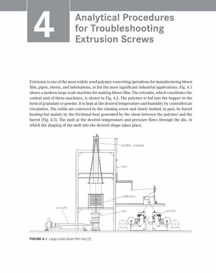
FIguRe 4.2  Extruder with auxialiary equipment [3]

 ■ 4.1  Three-Zone Screw

Basically extrusion consists of transporting the solid polymer in an extruder by means of a rotat-ing screw, melting the solid, homogenizing the melt, and forcing the melt through a die (Fig. 4.3).

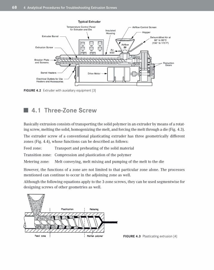
The extruder screw of a conventional plasticating extruder has three geometrically different zones (Fig. 4.4), whose functions can be described as follows:

Feed zone: Transport and preheating of the solid material

Transition zone: Compression and plastication of the polymer

Metering zone: Melt conveying, melt mixing and pumping of the melt to the die

However, the functions of a zone are not limited to that particular zone alone. The processes mentioned can continue to occur in the adjoining zone as well.

Although the following equations apply to the 3-zone screws, they can be used segmentwise for designing screws of other geometries as well.

FIguRe 4.3  Plasticating extrusion [4]

694.1 Three-Zone Screw

FIguRe 4.4  Three-zone screw [10]

4.1.1  extruder Output

Depending on the type of extruder, the output is determined either by the geometry of the solids feeding zone alone, as in the case of a grooved extruder [7], or by the solids and melt zones to be found in a smooth barrel extruder. A too high or too low output results when the dimensions of the screw and die are not matched with each other.

4.1.2  Feed Zone

A good estimate of the solids flow rate can be obtained from Eq. (4.1) as a function of the con-veying efficiency and the feed depth. The desired output can be found by simulating the effect of these factors on the flow rate by means of Eq. (4.1).

Calculated example

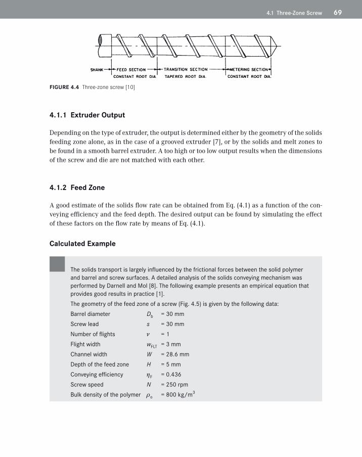
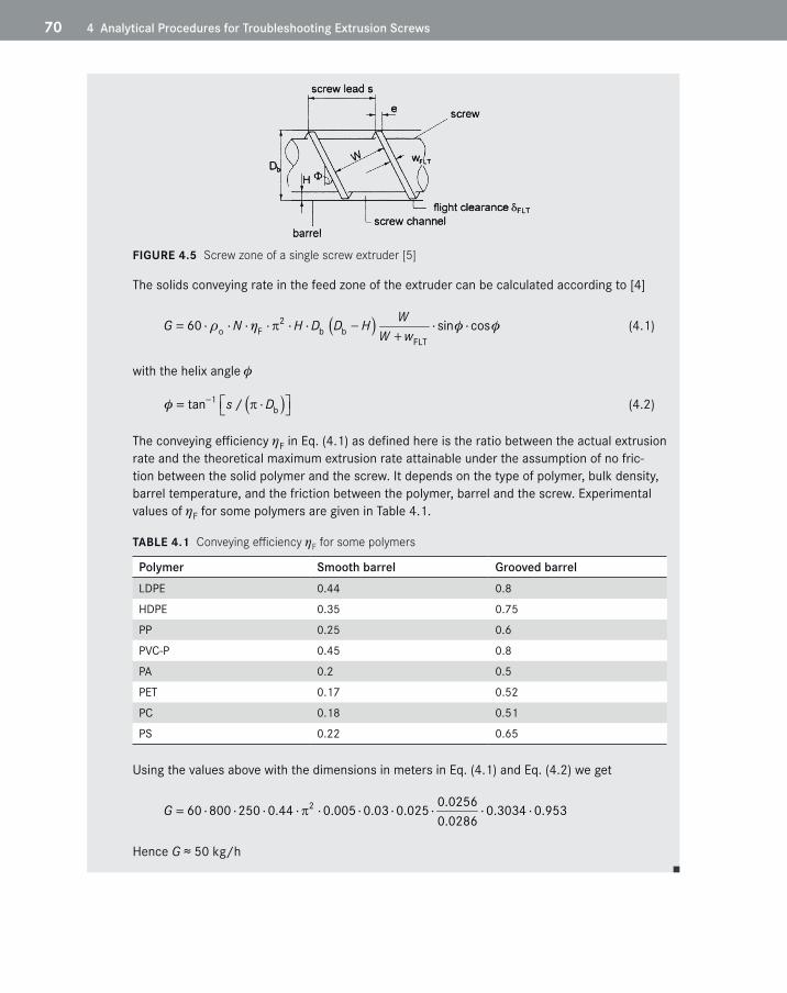
The solids transport is largely influenced by the frictional forces between the solid polymer and barrel and screw surfaces. A detailed analysis of the solids conveying mechanism was performed by Darnell and Mol [8]. The following example presents an empirical equation that provides good results in practice [1].The geometry of the feed zone of a screw (Fig. 4.5) is given by the following data:Barrel diameter Db = 30 mmScrew lead s = 30 mmNumber of flights = 1Flight width wFLT = 3 mmChannel width W = 28.6 mmDepth of the feed zone H = 5 mmConveying efficiency hF = 0.436Screw speed N = 250 rpmBulk density of the polymer ro = 800 kg/m3

70 4 Analytical Procedures for Troubleshooting Extrusion Screws

FIguRe 4.5  Screw zone of a single screw extruder [5]

The solids conveying rate in the feed zone of the extruder can be calculated according to [4]

( )r h π= ⋅ ⋅ ⋅ ⋅ ⋅ ⋅ − ⋅ ⋅+

2o F b b

FLT60 sin cosWG N H D D H

W w (4.1)

with the helix angle

( ) π− = ⋅ 1

btan /s D (4.2)

The conveying efficiency hF in Eq. (4.1) as defined here is the ratio between the actual extrusion rate and the theoretical maximum extrusion rate attainable under the assumption of no fric-tion between the solid polymer and the screw. It depends on the type of polymer, bulk density, barrel temperature, and the friction between the polymer, barrel and the screw. Experimental values of hF for some polymers are given in Table 4.1.

TAbLe 4.1  Conveying efficiency hF for some polymers

Polymer Smooth barrel Grooved barrelLDPE 0.44 0.8

HDPE 0.35 0.75

PP 0.25 0.6

PVC-P 0.45 0.8

PA 0.2 0.5

PET 0.17 0.52

PC 0.18 0.51

PS 0.22 0.65

Using the values above with the dimensions in meters in Eq. (4.1) and Eq. (4.2) we get

π= ⋅ ⋅ ⋅ ⋅ ⋅ ⋅ ⋅ ⋅ ⋅ ⋅2 0.025660 800 250 0.44 0.005 0.03 0.025 0.3034 0.9530.0286

G

Hence G ≈ 50 kg/h

1636.3 Injection Mold

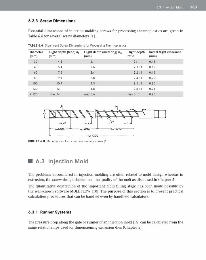
6.2.3  Screw Dimensions

Essential dimensions of injection molding screws for processing thermoplastics are given in Table 6.6 for several screw diameters [1].

TAbLe 6.6  Significant Screw Dimensions for Processing Thermoplastics

Diameter(mm)

Flight depth (feed) hF(mm)

Flight depth (metering) hM(mm)

Flight depth ratio

Radial flight clearance(mm)

30 4.3 2.1 2 : 1 0.15

40 5.4 2.6 2.1 : 1 0.15

60 7.5 3.4 2.2 : 1 0.15

80 9.1 3.8 2.4 : 1 0.20

100 10.7 4.3 2.5 : 1 0.20

120 12 4.8 2.5 : 1 0.25

> 120 max 14 max 5.6 max 3 : 1 0.25

FIguRe 6.8  Dimensions of an injection molding screw [1]

 ■ 6.3  Injection Mold

The problems encountered in injection molding are often related to mold design whereas in extrusion, the screw design determines the quality of the melt as discussed in Chapter 5.

The quantitative description of the important mold filling stage has been made possible by the well-known software MOLDFLOW [10]. The purpose of this section is to present practical calculation procedures that can be handled even by handheld calculators.

6.3.1  Runner Systems

The pressure drop along the gate or runner of an injection mold [15] can be calculated from the same relationships used for dimensioning extrusion dies (Chapter 5).

164 6 Analytical Procedures for Troubleshooting Injection Molding

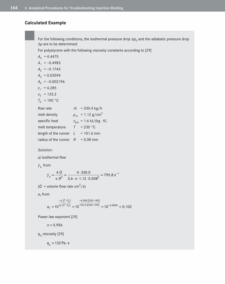
Calculated example

For the following conditions, the isothermal pressure drop Dp0 and the adiabatic pressure drop Dp are to be determined:For polystyrene with the following viscosity constants according to [29]A0 = 4.4475A1 = –0.4983A2 = –0.1743A3 = 0.03594A4 = –0.002196c1 = 4.285c2 = 133.2T0 = 190 °C

flow rate m = 330.4 kg/hmelt density rm = 1.12 g/cm3

specific heat cpm = 1.6 kJ/(kg · K)melt temperature T = 230 °Clength of the runner L = 101.6 mmradius of the runner R = 5.08 mm

Solution:

a) Isothermal flow

a from

π π

−⋅= = =⋅ ⋅ ⋅

1a 3 3

4 4 330.0 795.8 s3.6 1.12 0.508

QR

( Q = volume flow rate cm3/s)

aT from( )( )

( )( )

− − − −+ − + − −= = = =1 0

2 0

4.285 230 190133.2 230 190 0.9896

T 10 10 10 0.102

c T Tc T Ta

Power law exponent [29]

= 5.956n

ha, viscosity [29]

h = ⋅a 132 Pa s

1656.3 Injection Mold

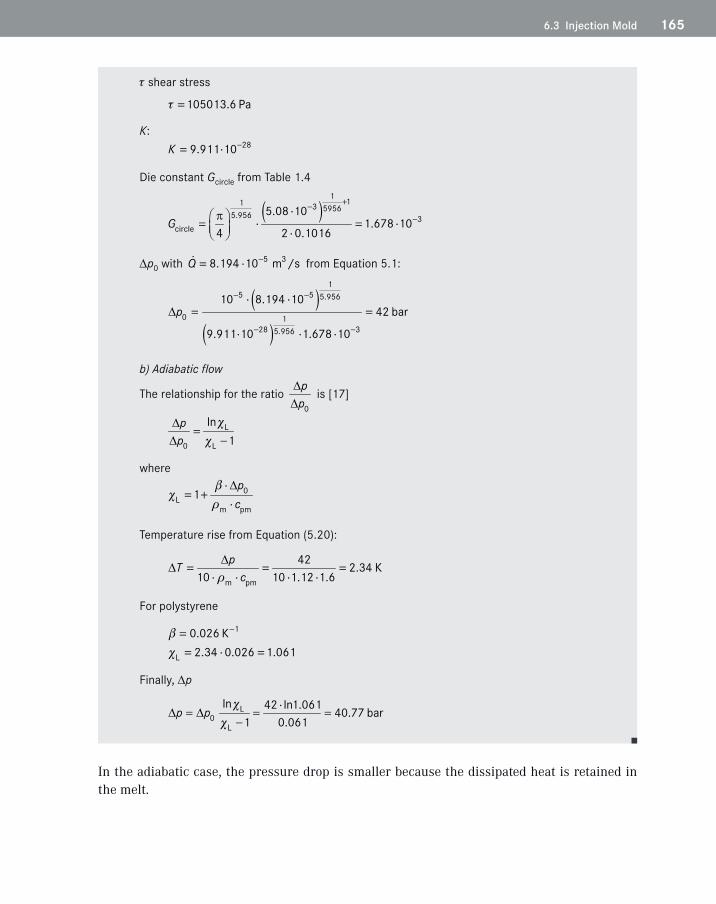
shear stress

=105013.6 Pa

K:−= ⋅ 289.911 10K

Die constant Gcircle from Table 1.4

( )π+−

−⋅

= ⋅ = ⋅ ⋅

1 11 3 59565.956 3

circle

5.08 101.678 10

4 2 0.1016G

Dp0 with −= ⋅

5 38.194 10 m /sQ from Equation 5.1:

( )( )

D− −

− −

⋅ ⋅= =

⋅ ⋅ ⋅

15 5 5.956

0 128 35.956

10 8.194 1042 bar

9.911 10 1.678 10

p

b) Adiabatic flow

The relationship for the ratio DD 0

pp

is [17]

DD

=−L

0 L

ln1

pp

where

r

D⋅= +

⋅0

Lm pm

1pc

Temperature rise from Equation (5.20):

rD

D = = =⋅ ⋅ ⋅ ⋅m pm

42 2.34 K10 10 1.12 1.6

pTc

For polystyrene

−== ⋅ =

1

L

0.026 K2.34 0.026 1.061

Finally, Dp

D D

⋅= = =−L

0L

ln 42 ln1.061 40.77 bar1 0.061

p p

In the adiabatic case, the pressure drop is smaller because the dissipated heat is retained in the melt.

166 6 Analytical Procedures for Troubleshooting Injection Molding

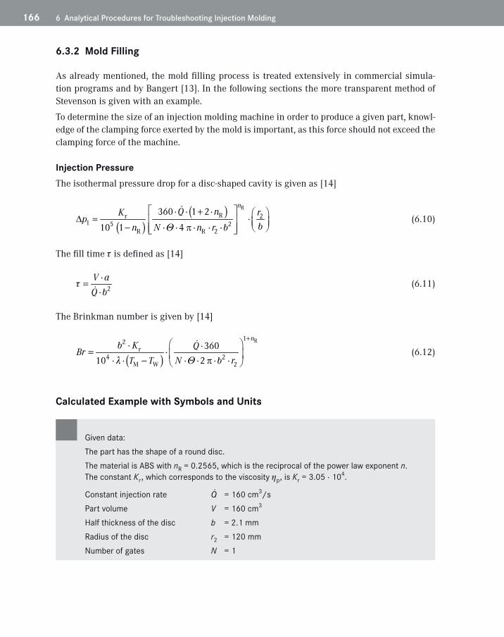
6.3.2  Mold Filling

As already mentioned, the mold filling process is treated extensively in commercial simula-tion programs and by Bangert [13]. In the following sections the more transparent method of Stevenson is given with an example.

To determine the size of an injection molding machine in order to produce a given part, knowl-edge of the clamping force exerted by the mold is important, as this force should not exceed the clamping force of the machine.

Injection PressureThe isothermal pressure drop for a disc-shaped cavity is given as [14]

( )( ) R

Rr 21 5 2

R R 2

360 1 2

10 1 4

nQ nK r

pbn N n r b

Dπ

⋅ ⋅ + ⋅ = ⋅ − ⋅ ⋅ ⋅ ⋅ ⋅ Θ

(6.10)

The fill time is defined as [14]

2V aQ b

⋅=⋅

(6.11)

The Brinkman number is given by [14]

( )R12

r4 2

M W 2

36010 2

nb K QBr

T T N b r π

+ ⋅ ⋅= ⋅ ⋅ ⋅ − ⋅ ⋅ ⋅ ⋅ Θ

(6.12)

Calculated example with Symbols and units

Given data:The part has the shape of a round disc.The material is ABS with nR = 0.2565, which is the reciprocal of the power law exponent n. The constant Kr, which corresponds to the viscosity hp, is Kr = 3.05 · 104.

Constant injection rate Q = 160 cm3/sPart volume V = 160 cm3

Half thickness of the disc b = 2.1 mmRadius of the disc r2 = 120 mmNumber of gates N = 1

1676.3 Injection Mold

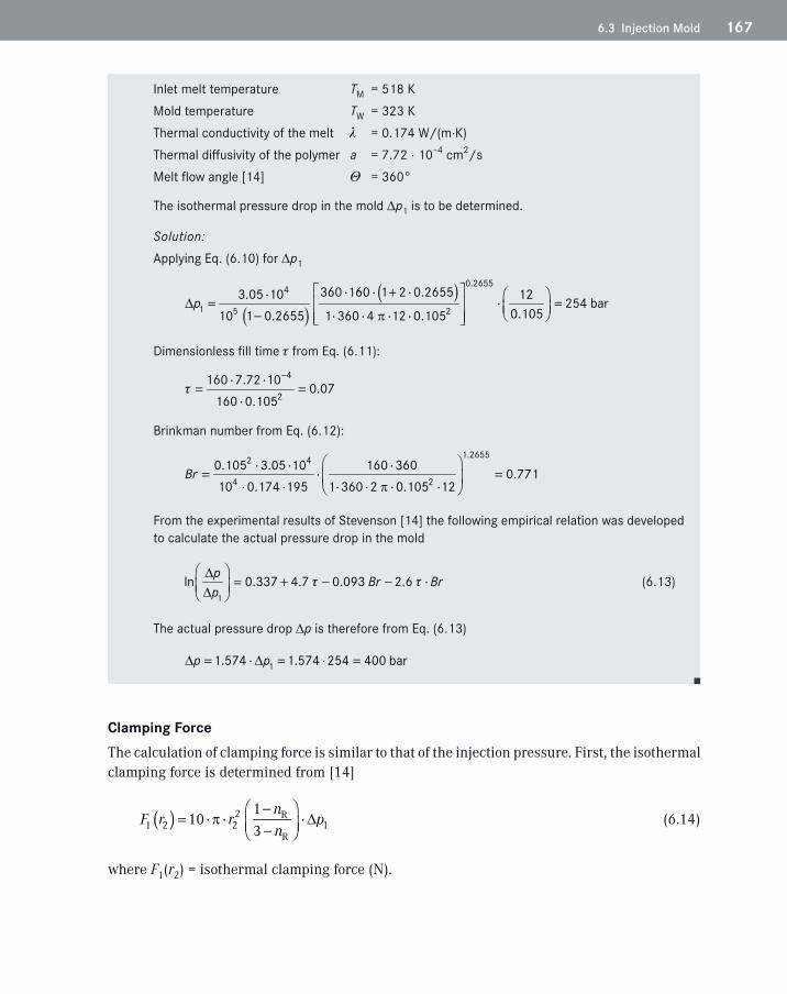
Inlet melt temperature TM = 518 KMold temperature TW = 323 KThermal conductivity of the melt = 0.174 W/(m·K)Thermal diffusivity of the polymer a = 7.72 · 10–4 cm2/sMelt flow angle [14] Θ = 360°

The isothermal pressure drop in the mold Dp1 is to be determined.

Solution:Applying Eq. (6.10) for Dp1

( )( )

Dπ

⋅ ⋅ + ⋅ ⋅= ⋅ = − ⋅ ⋅ ⋅ ⋅

0.26554

1 5 2

360 160 1 2 0.26553.05 10 12 254 bar0.10510 1 0.2655 1 360 4 12 0.105

p

Dimensionless fill time from Eq. (6.11):

−⋅ ⋅= =

⋅

4

2160 7.72 10 0.07

160 0.105

Brinkman number from Eq. (6.12):

π

⋅ ⋅ ⋅= ⋅ = ⋅ ⋅ ⋅ ⋅ ⋅ ⋅

1.26552 4

4 20.105 3.05 10 160 360 0.77110 0.174 195 1 360 2 0.105 12

Br

From the experimental results of Stevenson [14] the following empirical relation was developed to calculate the actual pressure drop in the mold

1ln 0.337 4.7 0.093 2.6p Br Br

p

DD

= + − − ⋅

(6.13)

The actual pressure drop Dp is therefore from Eq. (6.13)

11.574 1.574 254 400 barp pD D= ⋅ = ⋅ =

Clamping ForceThe calculation of clamping force is similar to that of the injection pressure. First, the isothermal clamping force is determined from [14]

( ) 2 R1 2 2 1

R

110

3n

F r r pn

π D −

= ⋅ ⋅ ⋅ − (6.14)

where F1(r2) = isothermal clamping force (N).

168 6 Analytical Procedures for Troubleshooting Injection Molding

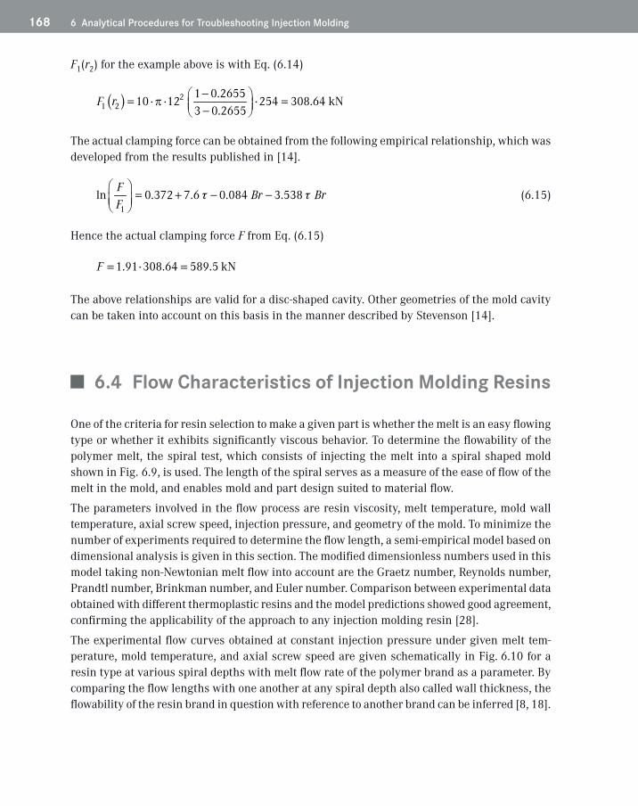
F1(r2) for the example above is with Eq. (6.14)

( ) 21 2

1 0.265510 12 254 308.64 kN

3 0.2655F r π

− = ⋅ ⋅ ⋅ = −

The actual clamping force can be obtained from the following empirical relationship, which was developed from the results published in [14].

1ln 0.372 7.6 0.084 3.538

F Br BrF

= + − − (6.15)

Hence the actual clamping force F from Eq. (6.15)

1.91 308.64 589.5 kNF = ⋅ =

The above relationships are valid for a disc-shaped cavity. Other geometries of the mold cavity can be taken into account on this basis in the manner described by Stevenson [14].

 ■ 6.4  Flow Characteristics of Injection Molding Resins

One of the criteria for resin selection to make a given part is whether the melt is an easy flowing type or whether it exhibits significantly viscous behavior. To determine the flowability of the polymer melt, the spiral test, which consists of injecting the melt into a spiral shaped mold shown in Fig. 6.9, is used. The length of the spiral serves as a measure of the ease of flow of the melt in the mold, and enables mold and part design suited to material flow.

The parameters involved in the flow process are resin viscosity, melt temperature, mold wall temperature, axial screw speed, injection pressure, and geometry of the mold. To minimize the number of experiments required to determine the flow length, a semi-empirical model based on dimensional analysis is given in this section. The modified dimensionless numbers used in this model taking non-Newtonian melt flow into account are the Graetz number, Reynolds number, Prandtl number, Brinkman number, and Euler number. Comparison between experimental data obtained with different thermoplastic resins and the model predictions showed good agreement, confirming the applicability of the approach to any injection molding resin [28].

The experimental flow curves obtained at constant injection pressure under given melt tem-perature, mold temperature, and axial screw speed are given schematically in Fig. 6.10 for a resin type at various spiral depths with melt flow rate of the polymer brand as a parameter. By comparing the flow lengths with one another at any spiral depth also called wall thickness, the flowability of the resin brand in question with reference to another brand can be inferred [8, 18].