Handling Practicalities in Agricultural PolicyOptimization for Water Quality Improvements

COIN Report Number 2017007

Brad Barnharta, Zhichao Lub, Moriah Bostianc, Ankur Sinhad, KalyanmoyDebb, Luba Kurkalovae, Manoj Jhae, Gerald Whittakerf

aU.S. EPA ORD NHEERL WEDbMichigan State University

cLewis & Clark CollegedIndian Institute of Management

eNorth Carolina A&TfOregon State University

Abstract

Bilevel and multi-objective optimization methods are often useful to spa-tially target agri-environmental policy throughout a watershed. This typeof problem is complex and is comprised of a number of practicalities: (i) alarge number of decision variables, (ii) at least two inter-dependent levels ofoptimization between policy makers and policy followers, and (iii) uncer-tainty in decision variables and problem parameters. Given agricultural andeconomic data from the Raccoon watershed in central Iowa, we formulate abilevel multi-objective optimization problem that accommodates objectivesof both policy makers and farmers. The solution procedure then explic-itly accounts for the nested nature of farm-level management decisions inresponse to agri-environmental policy incentives constructed by policy mak-ers. We specifically examine the spatial targeting of a fertilizer-reductionincentive policy while seeking to maximize farm-level productivity whilegenerating mandated water quality improvements using this framework.We test three different evolutionary optimization algorithms – m-BLEAQ,NSGA-II, and SPEA2 – and show that m-BLEAQ is well suited for handlingthe bilevel optimization problems and the considered practicalities.

1. Introduction

Nonpoint source pollution from agriculture remains a leading policychallenge for water quality improvement [23]. Key complicating factors

include measurement problems for emissions, spatial heterogeneity of pro-duction over the agricultural landscape, and the hydrological dynamicswithin the watershed [22]. One promising area of research in agriculturaland natural resource economics surrounds the use of integrated models thatlink management practices and production decisions to physical modelsof nutrient flow [25]. This integrated approach allows for optimal spatialtargeting of management practices over the agricultural landscape and moreexplicit estimation of policy cost [29, 8].

In general, problems involving players, where the actions of one player(leader) are followed by the optimal response from another player (fol-lower), are referred to as Stackelberg games. Such kind of games werefirst studied by Stackelberg [42]. Later in the 1970s, these problems wereformulated as nested mathematical programs [9] and found applications ina wide variety of areas like defense [11, 44], transportation [26, 10], modelproduction processes [27], chemical engineering [41, 12], and optimal taxpolicies [24, 34, 36], among others. A number of studies followed that in-cluded algorithms [3, 6, 4, 43, 45] These types of problems require nestedoptimization algorithms with one algorithm within the other, which leadsto high computational requirements. Recently, meta-modeling approacheshave gained importance for bilevel programming that exploit the propertiesof bilevel problems through mappings to solve the problem with lessercomputational expense. A few studies in this direction are [33, 35, 1, 40, 38].Multiobjective studies on bilevel optimization are few, both in the classical[16, 19] and evolutionary computation [47, 13, 37, 39] domain.

In this paper, we consider an agri-environmental policy targeting prob-lem for the Raccoon watershed in Central Iowa, USA. The upper leveldecision maker (i.e., the policy maker in this case) faces multiple objectivesof minimizing pollution and maximizing social benefit from agriculturalproduction. However, the policy maker is incapable of solving her ownoptimization problem without taking the actions of the followers (i.e., thefarmers) into account. For different policy decisions that the policy makermakes, the farmers react differently by maximizing their own objectives.This interaction makes the policy maker’s problem a nested optimizationtask with the farmers’ response embedded within the policy maker’s prob-lem. A deterministic version of this problem can be formulated as a bileveloptimization problem, which is a two level mathematical program with oneprogram nested within the other. A natural extension of a deterministicproblem is a problem that takes into account real-world uncertainties arisingfrom the uncertain behavior of the players and other environmental param-eters. We study both the deterministic as well as the uncertain version of

2

the agri-environmental policy targeting problem in this paper.We first provide a general formulation of a multiobjective bilevel prob-

lem, and one of the common techniques used to reduce it to a single-levelproblem. Thereafter, we discuss the agri-environmental policy targetingproblem and provide its empirical models. Specifically, an empirical modelfor farm-level profits and yield is introduced along with another empiricalecohydrological model for the Raccoon watershed that we use to simulatethe effects of fertilizer usage on water quality at the outlet of the watershed.Though the model considered in this paper has a bilevel structure, the regu-larity of the lower level allows us to write the problem as a multiobjectiveoptimization problem. This allows us to solve the problem using a standardmultiobjective optimizer when the optimal solution to the lower level can bewritten in closed form. We also solve the problem with a bilevel multiobjec-tive evolutionary optimization algorithm to which the lower level optimalsolution is not available directly. We compare the results for the two ap-proaches and then incorporate additional real-world difficulties (risk-baseduncertainties) in the model. Finally, we end the paper with some insights onfuture studies and conclusions.

2. Multiobjective Bilevel Model for Policy Problems

In this section, we provide a general formulation for policy problemswhere the upper level decision maker (policy maker) faces multiple objec-tives and the lower level decision maker faces a single objective. In othercases, where the lower level decision maker also has multiple objectives, thelower level problem can be replaced with a value function correspondingto the lower level decision maker, thereby reducing the lower level prob-lem to a single objective optimization task. A bilevel problem has decisionvariables, constraints and objectives corresponding to each player. The con-straints and objectives for each level may involve decision variables of theother player, thereby making the two levels interdependent. The lower leveloptimization is a parametric optimization task for which the upper levelvariables act as parameters, and the problem must be solved with respect tothe lower level variables. Assuming a single leader and a single follower,the problem can be defined as follows:

Definition 1. For the upper-level objective function F : Rn ×Rm → Rp andlower-level objective function f : Rn ×Rm → R, the bilevel optimization

3

problem is given as:

minimizex,y

F(x, y) = (F1(x, y), . . . , Fp(x, y))

subject toy ∈ argmin

y f (x, y) : gj(x, y) ≤ 0, j = 1, . . . , J

Gl(x, y) ≤ 0, l = 1, . . . , L

where Gl : Rn ×Rm → R, l = 1, . . . , L denotes the upper level constraints,and gj : Rn ×Rm → R, j = 1, . . . , J represents the lower level constraints.

The agri-envorinmental policy targeting problem is a different bilevel prob-lem in which there are multiple followers, each acting independently andrationally, after the decisions of the leader. In such a case, the respectivebilevel problem gets modified as:

Definition 2. For the upper-level objective function F : Rn ×Rm → Rp

corresponding to a single leader and lower level objective functions fk : Rn×Rm → R corresponding to followers k ∈ 1, . . . , K, the bilevel optimizationproblem with single leader and multiple follower is given as:

minimizex,y

(F1(x, y1, . . . , yK), . . . , Fp(x, y1, . . . , yK)

subject to

y1 ∈ argminy1 f 1(x, yk) : g1

j (x, y1) ≤ 0, j = 1, . . . , J

y2 ∈ argminy2 f 2(x, yk) : g2

j (x, y2) ≤ 0, j = 1, . . . , J

...

yk ∈ argminyk f k(x, yk) : gK

j (x, yk) ≤ 0, j = 1, . . . , J

Gl(x, y1, . . . , yK) ≤ 0, l = 1, . . . , L

where Gl : Rn ×Rm → R, l = 1, . . . , L denotes the upper level constraints,and gk j : Rn ×Rm → R, j = 1, . . . , J represents the lower level constraintsfor followers k ∈ 1, . . . , K, respectively.

Due to the presence of multiple followers each involving a different op-timization problem, this problem is more computationally challenging tosolve than the usual bilevel problems presented in Definition 1.

4

2.1. Single Level ReductionIn bilevel optimization, it is possible to replace the lower level problems

in Definitions 1 and 2 with its Karush-Kuhn-Tucker (KKT) conditions whenthe lower level problems adhere to certain regularity conditions. Despitethe reduction to single level, such problems are still hard to handle becauseof the constrained search space induced because of the KKT conditions. Incertain situations, it might even be possible to write the optimal solution tothe lower level problem in a closed form, i.e. y(x); however, this is rare. If aclosed form solution can be written, then the bilevel problem effectively getsreduced to an ordinary optimization task. For multiple-follower problems,closed form optimal solutions or any approximations to the lower levelproblem are extremely beneficial.

3. Agri-environmental Policy Targeting Problem

Next, we consider our agri-environmental policy targeting problem forthe Raccoon River Watershed, which covers roughly 9,400 km2 in West-Central Iowa.

Agriculture accounts for the majority of land use in the study area, with75.3% of land in cropland, 16.3% in grassland, 4.4% in forests and just 4% inurban use [20]. The watershed has been widely studied [20, 17, 21], and morerecently in a bilevel framework [7], due to its high concentration of nitratepollution from intensive fertilizer and livestock manure application. Nitrateconcentrations routinely exceed Federal limits, with citations dating backto the late 1980s. The watershed also serves as the main source of drinkingwater for more than 500,000 people in Central Iowa. As a consequence,the Des Moines Water Works (DMWW) has for many years operated theworld’s largest nitrate removal facility. In 2015, a spike in nitrate levelsforced the facility to run its nitrate removal equipment for a record 177 days.This culminated in the well-publicized federal lawsuit filed that year by theDMWW against three area counties for failing to control nitrate pollutionfrom agricultural non-point sources.

3.1. Problem formulationGiven the above issues, one of the objectives the policy maker faces is to

reduce the extent of pollution caused by agricultural activities by controllingthe amount of fertilizer used. However, at the same time the policy makerdoes not intend to hamper agricultural activities to an extent of causingsignificant economic distress for the farmers.

5

Consider a producer (follower) k ∈ 1, . . . , K trying to maximize herprofits from agricultural production through N inputs xk = xk

1, ..., xkN

and M outputs yk = yk1, ..., yk

M. Out of the N inputs, xkN denotes the

fertilizer input for each farm. The policy maker must choose the optimalspatial allocation of taxes, τ = τ1, . . . , τK, for each farm correspondingto the Nitrogen fertilizer usage xN = xk

N , . . . , xkN so as to control the

use of fertilizers. Tax vector τ = τ1, . . . , τK denotes the tax policy for Kproducers that is expressed as a multiplier on the total cost of fertilizers. Notethat the taxes can be applied as a constant for the entire basin, or they can bespatially targeted at semi-aggregated levels or individually at the farm-level.For generality, in our model we have assumed a different tax policy foreach producer. The objectives of the upper level are to to jointly maximizeenvironmental benefits, B(xN)—which consists of the total reduction of non-point source emissions of Nitrogen runoff from agricultural land—while alsomaximizing the total basin’s profit Π(τ, x, y). The optimization problem thatthe policy maker needs to solve in order to identify a Pareto set of efficientpolicies is given as follows:

maxτ,x,y

F(τ, x) =(Π(τ, xN), B(xN)

)(1)

s.t. (xk, yk) ∈ argmaxxk , yk

πk(τk, xk, yk) : (τk, xk, yk) ∈ Ωk

∀ k ∈ 1, . . . , K,xk

n ≥ 0, ∀ k ∈ 1, . . . , K, n ∈ 1, . . . , N,yk

m ≥ 0, ∀ k ∈ 1, . . . , K, m ∈ 1, . . . , M,τk ≥ 1, ∀ k ∈ 1, . . . , K,

(2)

The fertilizer tax, τ, serves as a multiplier on the total cost of fertilizer,so that τ ≥ 1. The environmental benefit is the negative of pollutionand therefore can be written as the negative of the total pollution causedby the producers, i.e. B(xN) = −∑K

k=1 p(xkN). Similarly the total basin

profit can be written as the sum total of individual producer’s profit, i.e.Π(τ, x, y) = ∑K

k=1 π(τk, xk, yk). The lower level optimization problem foreach agricultural producer can be written as:

maxxk ,yk

πk(pk, wk, τk) = pkyk −N−1

∑n=1

wnxkn − τk

NwNxkN (3)

s.t. yk ≤ Pk(xk),

6

where w and p are the costs and prices of the inputs x and outputs y, respec-tively. Pk(xk) denotes the production frontier for producer k. Heterogeneityacross producers, due primarily to differences in soil type, may prevent theuse of a common production function that would simplify the solution of (1).Likewise, the environmental benefits of reduced fertilizer use vary acrossproducers, due to location and hydrologic processes within the basin. Thisalso makes the solution of (1) more complex.

3.2. Empirical Model for Iowa Crop ProductionThe Iowa crop production model [32] is used to analytically model the

economics of agricultural producers in the Raccoon watershed. The modeloperates on a 56 meter square grid based on USDA GIS remote-sensingcrop cover maps. To account for producer heterogeneity across grid units,we use the ICCPI soil quality index, a measure of soil productivity thatcomes from GIS-based soil data. We model three crop rotations currentlypracticed in Iowa: continuous corn, corn-soybeans, and corn-corn-soybeans.The model captures the differentiated impacts of rotations on the yields.Crop production outputs, ym, m = 1 (corn), 2 (soybeans), are expressedas functions of soil productivity, q, previous crop, tillage system, s, andnitrogen fertilizer application, xN .

The corresponding corn and soybean current yield functions, in bushelsper acre, are:

yk1 = qk[α0γ

sk2

2 γsk

33 γ

(1−dkc)s2

4 γ5(1−dkc)sk

3 + α1dkc

+α2(x− ρdkc) + α3(xk

N − ρdkc)

2](4)

andyk

2 = qk[α0γsk

22 γ

sk3

3 + α1dkc + α2dk

cc], (5)

where dc indicates corn as the previous crop, dcc indicates corn as the pre-vious two crops, s2 indicates mulch as the tillage choice, and s3 indicatesno-till as the tillage choice. The ICCPI productivity measure, q, serves as amultiplier, ranging from 0 to 1. There are three possible rotations: corn-corn(cc), corn-soy (cs), corn-corn-soy (ccs). Note that nitrogen fertilizer is onlyapplied to corn, and that current yields depend on position within a givenrotation.

Given the above functions, the optimal response of the followers canbe written as a closed form solution in terms of the upper level decisionvariables. Profit maximization implies the optimal nitrogen fertilizer inputdemands as

xk∗N = ρ +

τNwN

p12α3qk −α2

2α3, (6)

7

for corn after corn, and

xk∗N =

τNwN

p12α3qk −α2

2α3, (7)

for corn after soy.

3.3. The Biophysical ModelTo model the water quality effects of prospective policy incentive schemes,

we input the corresponding production model’s fertilizer use into an em-pirical model for producing Nitrogen run-off. The model is runoffk =

e−0.9819+1.668 log(1.12085xkN) [46]. The sum of all runoff from all farms is defined

to be the runoff for the entire basin, which is minimized as an upper levelobjective. In our future work we intend to utilize a more accurate spatiallyexplicit biophysical watershed model known as the Soil and Water Assess-ment Tool (SWAT) [2] to dynamically simulate Nitrogen runoff at the basin’soutlet using local information related to land cover, soil type, and watermanagement practices (e.g., tile drains). A number of studies apply SWATto non-point policy for this reason [5, 31, 30].

4. Computational Algorithms Used in this Study

We use three different approaches to identify the Pareto-optimal set ofpolicies for the upper level decision maker. In this section, we provide abrief description of the approaches that we have used to solve the aboveproblem.

4.1. DEAP ImplementationOur first approach implements the Distributed Evolutionary Algorithms

in Python (DEAP) [18], which is a flexible optimization framework. Weused the traditional (µ + λ) evolutionary algorithm with SPEA2 selection[48] using DEAP. The algorithm creates a parent population of µ individualsand subsequently generates λ offspring within the population. After (µ + λ)individuals are tested, the results are sorted, and the µ best individualsfrom the (µ + λ) population are selected for the next generation. For thisapplication, we set µ = 100 and λ = 100; these values were chosen toproduce a suitably large population without incurring substantial computa-tional burden. Crossover and mutation probabilities were set to 0.90 and1/(number of farms), respectively, following conventions [18]. DEAP ishighly integrated with the SCOOP library in Python [28], which enablesparallel implementation of the algorithm to reduce computational burden.

8

4.2. m-BLEAQ ImplementationThe second approach utilizes m-BLEAQ [39]. The algorithm draws

insights from the mathematical structure and properties of bilevel optimiza-tion problems and attempts to reduce the computational costs. The methodcreates localized quadratic approximations of the rational reaction set of thefollowers as a function of the leader’s decision variables. This helps in reduc-ing the number of lower level optimization calls that are required to solvethe bilevel optimization problem. If the localized quadratic approximationof the rational reaction set created by the algorithm is accurate, then theoptimal response of the follower in the vicinity of the local approximationcan be directly obtained by using the approximation instead of solving thelower level optimization problem. Such local approximations of the rationalreaction set are useful to guide the algorithm to the regions that might con-tain the bilevel optimal solutions without wasting computations in poorerregions. As the population members converge towards the Pareto-optimalsolutions, the approximation continues to improve. In this study, whileusing m-BLEAQ we do not provide the algorithm the lower level optimalsolutions; instead, we let the algorithm handle the entire bilevel problem.

4.3. NSGA-II ImplementationWe also use NSGA-II [15] to solve the bilevel problem in this study.

Since NSGA-II is capable of handling single level multi-objective problems,we therefore eliminate the lower level completely and directly provide theoptimal lower level solution to the upper level using the empirical solutionsin 6 and 7.

5. Results

In this section, we provide the simulation results comparing m-BLEAQ,NSGA-II, and SPEA2 on the empirical model of the Iowa Racoon watershed.Results on a small size, scaled size of the problem, robustness study will beillustrated one at a time in the following of the section.

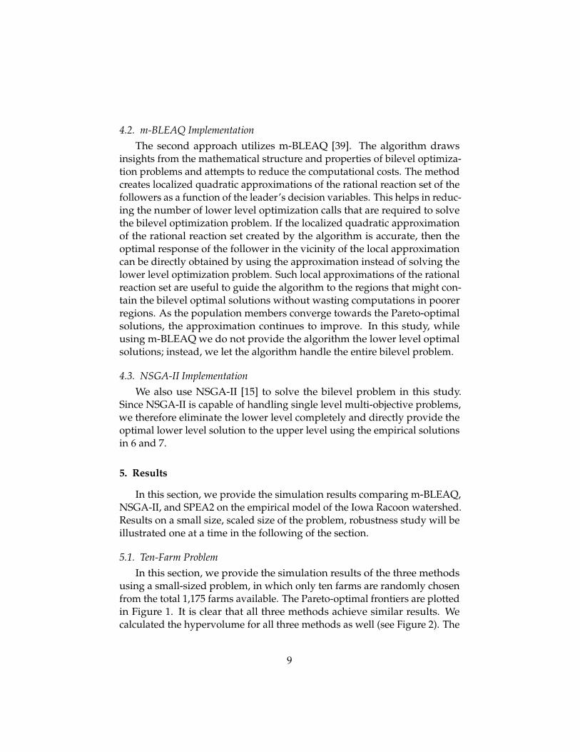
5.1. Ten-Farm ProblemIn this section, we provide the simulation results of the three methods

using a small-sized problem, in which only ten farms are randomly chosenfrom the total 1,175 farms available. The Pareto-optimal frontiers are plottedin Figure 1. It is clear that all three methods achieve similar results. Wecalculated the hypervolume for all three methods as well (see Figure 2). The

9

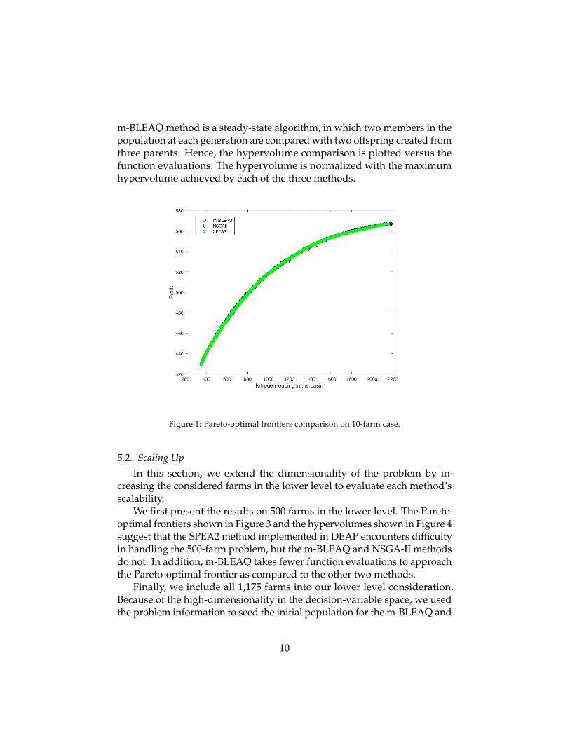
m-BLEAQ method is a steady-state algorithm, in which two members in thepopulation at each generation are compared with two offspring created fromthree parents. Hence, the hypervolume comparison is plotted versus thefunction evaluations. The hypervolume is normalized with the maximumhypervolume achieved by each of the three methods.

Figure 1: Pareto-optimal frontiers comparison on 10-farm case.

5.2. Scaling UpIn this section, we extend the dimensionality of the problem by in-

creasing the considered farms in the lower level to evaluate each method’sscalability.

We first present the results on 500 farms in the lower level. The Pareto-optimal frontiers shown in Figure 3 and the hypervolumes shown in Figure 4suggest that the SPEA2 method implemented in DEAP encounters difficultyin handling the 500-farm problem, but the m-BLEAQ and NSGA-II methodsdo not. In addition, m-BLEAQ takes fewer function evaluations to approachthe Pareto-optimal frontier as compared to the other two methods.

Finally, we include all 1,175 farms into our lower level consideration.Because of the high-dimensionality in the decision-variable space, we usedthe problem information to seed the initial population for the m-BLEAQ and

10

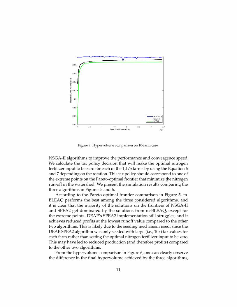
Figure 2: Hypervolume comparison on 10-farm case.

NSGA-II algorithms to improve the performance and convergence speed.We calculate the tax policy decision that will make the optimal nitrogenfertilizer input to be zero for each of the 1,175 farms by using the Equation 6and 7 depending on the rotation. This tax policy should correspond to one ofthe extreme points on the Pareto-optimal frontier that minimize the nitrogenrun-off in the watershed. We present the simulation results comparing thethree algorithms in Figures 5 and 6.

According to the Pareto-optimal frontier comparison in Figure 5, m-BLEAQ performs the best among the three considered algorithms, andit is clear that the majority of the solutions on the frontiers of NSGA-IIand SPEA2 get dominated by the solutions from m-BLEAQ, except forthe extreme points. DEAP’s SPEA2 implementation still struggles, and itachieves reduced profits at the lowest runoff value compared to the othertwo algorithms. This is likely due to the seeding mechanism used, since theDEAP SPEA2 algorithm was only seeded with large (i.e., 10x) tax values foreach farm rather than setting the optimal nitrogen fertilizer input to be zero.This may have led to reduced production (and therefore profits) comparedto the other two algorithms.

From the hypervolume comparison in Figure 6, one can clearly observethe difference in the final hypervolume achieved by the three algorithms,

11

Figure 3: Pareto-optimal frontiers comparison on 500 farms case

and surprisingly m-BLEAQ could still approach the Pareto-optimal frontierwith very few function evaluations.

5.3. Effect of Recombination Operators in NSGA-IIThe dramatic difference between the results obtained from m-BLEAQ

and NSGA-II is surprising to the investigators since the m-BLEAQ solutionprocedure is very similar to NSGA-II when the lower level optimal reactionfunction is readily available. Despite the steady-state nature, m-BLEAQ usesa vector-wise recombination operator, Parent Centric Crossover (PCX), thatis different from the variable-wise recombination operator, Simulated BinaryCrossover (SBX), used in NSGA-II. Also, studies have shown that PCX issuperior to SBX in handling variable linkages and complex problems [14].Therefore, we now compare NSGA-II, NSGA-II with PCX, and m-BLEAQ tofurther validate this finding.

It is clear from Figure 7 that the variable-wise recombination operatorcannot properly handle the high-dimensionality in the problem, but a vector-wise recombination (PCX) using NSGA-II achieves similar results to thatobtained by the bilevel m-BLEAQ approach.

12

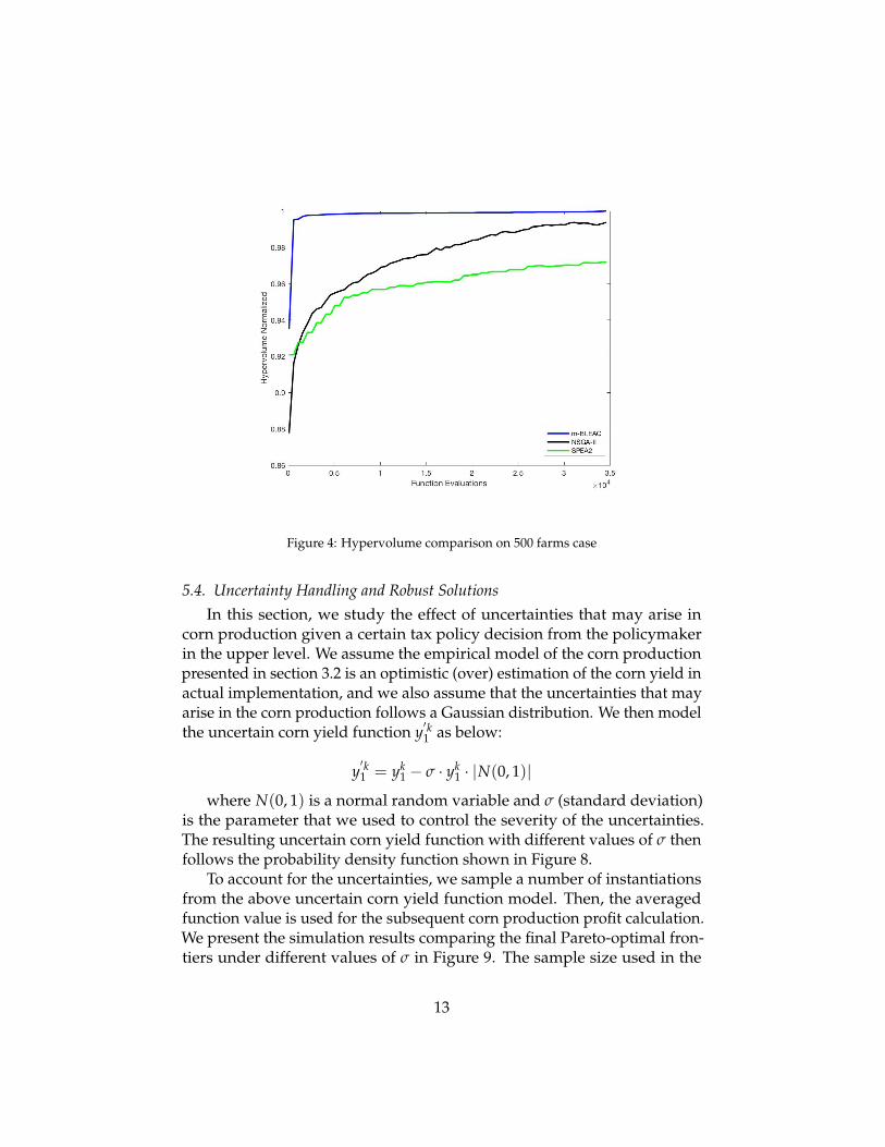
Figure 4: Hypervolume comparison on 500 farms case

5.4. Uncertainty Handling and Robust SolutionsIn this section, we study the effect of uncertainties that may arise in

corn production given a certain tax policy decision from the policymakerin the upper level. We assume the empirical model of the corn productionpresented in section 3.2 is an optimistic (over) estimation of the corn yield inactual implementation, and we also assume that the uncertainties that mayarise in the corn production follows a Gaussian distribution. We then modelthe uncertain corn yield function y

′k1 as below:

y′k1 = yk

1 − σ · yk1 · |N(0, 1)|

where N(0, 1) is a normal random variable and σ (standard deviation)is the parameter that we used to control the severity of the uncertainties.The resulting uncertain corn yield function with different values of σ thenfollows the probability density function shown in Figure 8.

To account for the uncertainties, we sample a number of instantiationsfrom the above uncertain corn yield function model. Then, the averagedfunction value is used for the subsequent corn production profit calculation.We present the simulation results comparing the final Pareto-optimal fron-tiers under different values of σ in Figure 9. The sample size used in the

13

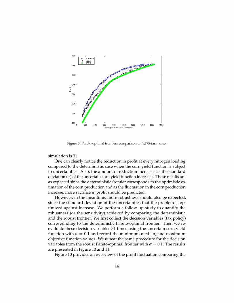
Figure 5: Pareto-optimal frontiers comparison on 1,175-farm case.

simulation is 31.One can clearly notice the reduction in profit at every nitrogen loading

compared to the deterministic case when the corn yield function is subjectto uncertainties. Also, the amount of reduction increases as the standarddeviation (σ) of the uncertain corn yield function increases. These results areas expected since the deterministic frontier corresponds to the optimistic es-timation of the corn production and as the fluctuation in the corn productionincrease, more sacrifice in profit should be predicted.

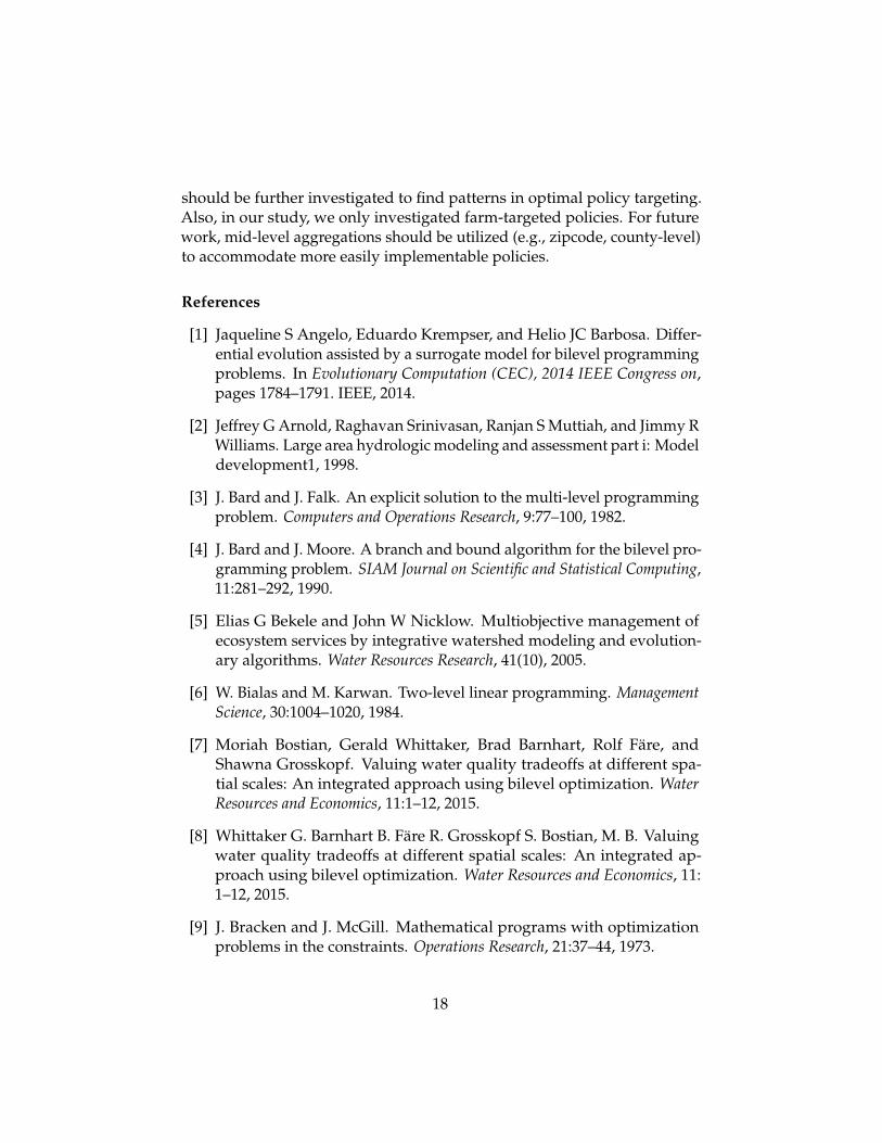
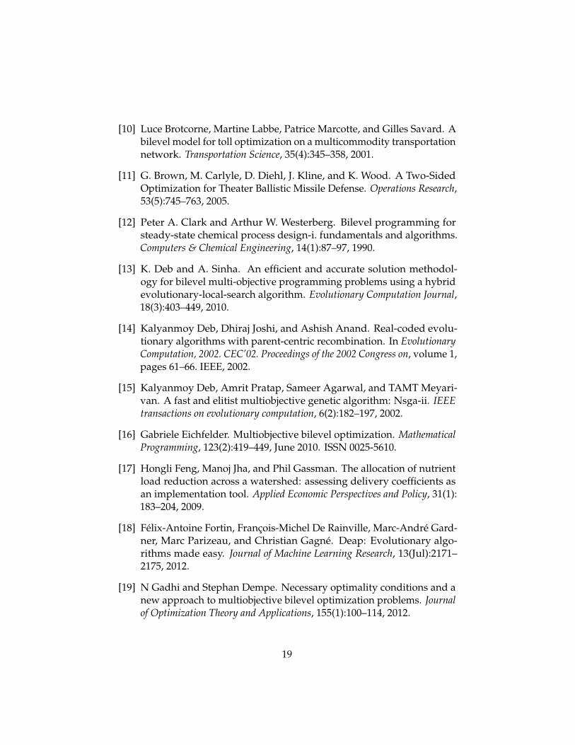
However, in the meantime, more robustness should also be expected,since the standard deviation of the uncertainties that the problem is op-timized against increase. We perform a follow-up study to quantify therobustness (or the sensitivity) achieved by comparing the deterministicand the robust frontier. We first collect the decision variables (tax policy)corresponding to the deterministic Pareto-optimal frontier. Then we re-evaluate these decision variables 31 times using the uncertain corn yieldfunction with σ = 0.1 and record the minimum, median, and maximumobjective function values. We repeat the same procedure for the decisionvariables from the robust Pareto-optimal frontier with σ = 0.1. The resultsare presented in Figure 10 and 11.

Figure 10 provides an overview of the profit fluctuation comparing the

14

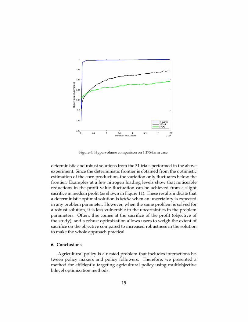
Figure 6: Hypervolume comparison on 1,175-farm case.

deterministic and robust solutions from the 31 trials performed in the aboveexperiment. Since the deterministic frontier is obtained from the optimisticestimation of the corn production, the variation only fluctuates below thefrontier. Examples at a few nitrogen loading levels show that noticeablereductions in the profit value fluctuation can be achieved from a slightsacrifice in median profit (as shown in Figure 11). These results indicate thata deterministic optimal solution is brittle when an uncertainty is expectedin any problem parameter. However, when the same problem is solved fora robust solution, it is less vulnerable to the uncertainties in the problemparameters. Often, this comes at the sacrifice of the profit (objective ofthe study), and a robust optimization allows users to weigh the extent ofsacrifice on the objective compared to increased robustness in the solutionto make the whole approach practical.

6. Conclusions

Agricultural policy is a nested problem that includes interactions be-tween policy makers and policy followers. Therefore, we presented amethod for efficiently targeting agricultural policy using multiobjectivebilevel optimization methods.

15

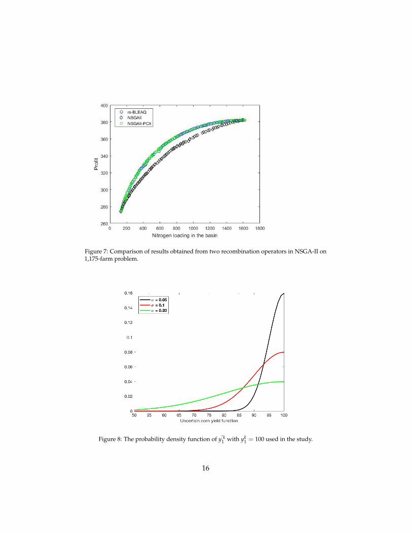
Figure 7: Comparison of results obtained from two recombination operators in NSGA-II on1,175-farm problem.

Figure 8: The probability density function of y′k1 with yk

1 = 100 used in the study.

16

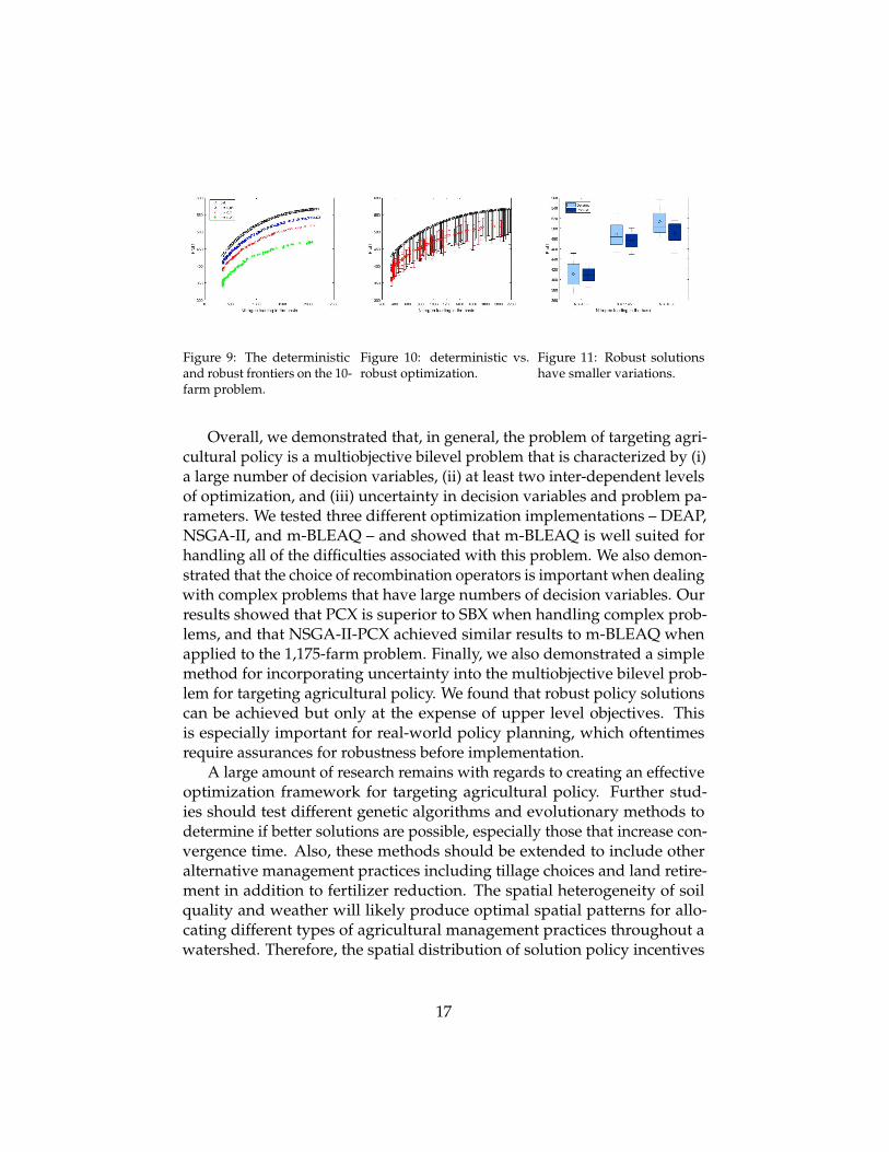
Figure 9: The deterministicand robust frontiers on the 10-farm problem.

Figure 10: deterministic vs.robust optimization.

Figure 11: Robust solutionshave smaller variations.

Overall, we demonstrated that, in general, the problem of targeting agri-cultural policy is a multiobjective bilevel problem that is characterized by (i)a large number of decision variables, (ii) at least two inter-dependent levelsof optimization, and (iii) uncertainty in decision variables and problem pa-rameters. We tested three different optimization implementations – DEAP,NSGA-II, and m-BLEAQ – and showed that m-BLEAQ is well suited forhandling all of the difficulties associated with this problem. We also demon-strated that the choice of recombination operators is important when dealingwith complex problems that have large numbers of decision variables. Ourresults showed that PCX is superior to SBX when handling complex prob-lems, and that NSGA-II-PCX achieved similar results to m-BLEAQ whenapplied to the 1,175-farm problem. Finally, we also demonstrated a simplemethod for incorporating uncertainty into the multiobjective bilevel prob-lem for targeting agricultural policy. We found that robust policy solutionscan be achieved but only at the expense of upper level objectives. Thisis especially important for real-world policy planning, which oftentimesrequire assurances for robustness before implementation.

A large amount of research remains with regards to creating an effectiveoptimization framework for targeting agricultural policy. Further stud-ies should test different genetic algorithms and evolutionary methods todetermine if better solutions are possible, especially those that increase con-vergence time. Also, these methods should be extended to include otheralternative management practices including tillage choices and land retire-ment in addition to fertilizer reduction. The spatial heterogeneity of soilquality and weather will likely produce optimal spatial patterns for allo-cating different types of agricultural management practices throughout awatershed. Therefore, the spatial distribution of solution policy incentives

17

should be further investigated to find patterns in optimal policy targeting.Also, in our study, we only investigated farm-targeted policies. For futurework, mid-level aggregations should be utilized (e.g., zipcode, county-level)to accommodate more easily implementable policies.

References

[1] Jaqueline S Angelo, Eduardo Krempser, and Helio JC Barbosa. Differ-ential evolution assisted by a surrogate model for bilevel programmingproblems. In Evolutionary Computation (CEC), 2014 IEEE Congress on,pages 1784–1791. IEEE, 2014.

[2] Jeffrey G Arnold, Raghavan Srinivasan, Ranjan S Muttiah, and Jimmy RWilliams. Large area hydrologic modeling and assessment part i: Modeldevelopment1, 1998.

[3] J. Bard and J. Falk. An explicit solution to the multi-level programmingproblem. Computers and Operations Research, 9:77–100, 1982.

[4] J. Bard and J. Moore. A branch and bound algorithm for the bilevel pro-gramming problem. SIAM Journal on Scientific and Statistical Computing,11:281–292, 1990.

[5] Elias G Bekele and John W Nicklow. Multiobjective management ofecosystem services by integrative watershed modeling and evolution-ary algorithms. Water Resources Research, 41(10), 2005.

[6] W. Bialas and M. Karwan. Two-level linear programming. ManagementScience, 30:1004–1020, 1984.

[7] Moriah Bostian, Gerald Whittaker, Brad Barnhart, Rolf Färe, andShawna Grosskopf. Valuing water quality tradeoffs at different spa-tial scales: An integrated approach using bilevel optimization. WaterResources and Economics, 11:1–12, 2015.

[8] Whittaker G. Barnhart B. Färe R. Grosskopf S. Bostian, M. B. Valuingwater quality tradeoffs at different spatial scales: An integrated ap-proach using bilevel optimization. Water Resources and Economics, 11:1–12, 2015.

[9] J. Bracken and J. McGill. Mathematical programs with optimizationproblems in the constraints. Operations Research, 21:37–44, 1973.

18

[10] Luce Brotcorne, Martine Labbe, Patrice Marcotte, and Gilles Savard. Abilevel model for toll optimization on a multicommodity transportationnetwork. Transportation Science, 35(4):345–358, 2001.

[11] G. Brown, M. Carlyle, D. Diehl, J. Kline, and K. Wood. A Two-SidedOptimization for Theater Ballistic Missile Defense. Operations Research,53(5):745–763, 2005.

[12] Peter A. Clark and Arthur W. Westerberg. Bilevel programming forsteady-state chemical process design-i. fundamentals and algorithms.Computers & Chemical Engineering, 14(1):87–97, 1990.

[13] K. Deb and A. Sinha. An efficient and accurate solution methodol-ogy for bilevel multi-objective programming problems using a hybridevolutionary-local-search algorithm. Evolutionary Computation Journal,18(3):403–449, 2010.

[14] Kalyanmoy Deb, Dhiraj Joshi, and Ashish Anand. Real-coded evolu-tionary algorithms with parent-centric recombination. In EvolutionaryComputation, 2002. CEC’02. Proceedings of the 2002 Congress on, volume 1,pages 61–66. IEEE, 2002.

[15] Kalyanmoy Deb, Amrit Pratap, Sameer Agarwal, and TAMT Meyari-van. A fast and elitist multiobjective genetic algorithm: Nsga-ii. IEEEtransactions on evolutionary computation, 6(2):182–197, 2002.

[16] Gabriele Eichfelder. Multiobjective bilevel optimization. MathematicalProgramming, 123(2):419–449, June 2010. ISSN 0025-5610.

[17] Hongli Feng, Manoj Jha, and Phil Gassman. The allocation of nutrientload reduction across a watershed: assessing delivery coefficients asan implementation tool. Applied Economic Perspectives and Policy, 31(1):183–204, 2009.

[18] Félix-Antoine Fortin, François-Michel De Rainville, Marc-André Gard-ner, Marc Parizeau, and Christian Gagné. Deap: Evolutionary algo-rithms made easy. Journal of Machine Learning Research, 13(Jul):2171–2175, 2012.

[19] N Gadhi and Stephan Dempe. Necessary optimality conditions and anew approach to multiobjective bilevel optimization problems. Journalof Optimization Theory and Applications, 155(1):100–114, 2012.

19

[20] Manoj K Jha, Philip Walter Gassman, and Jeffrey G Arnold. Water qual-ity modeling for the raccoon river watershed using swat. Transactionsof the ASAE, 50(2):479–493, 2007.

[21] Manoj K Jha, Calvin F Wolter, Keith E Schilling, and Philip W Gassman.Assessment of total maximum daily load implementation strategies fornitrate impairment of the raccoon river, iowa. Journal of EnvironmentalQuality, 39(4):1317–1327, 2010.

[22] C.L. Kling. Economic incentives to improve water quality in agri-cultural landscapes: Some new variations on old ideas. Journal ofAgricultural Economics, 93(2):297–309, 2011.

[23] L.A. Kurkalova. Cost-effective placement of best management practicesin a watershed: lessons learned from Conservation Effects AssessmentProject. Journal of the American Water Resources Association, 51(2):359–372,2015.

[24] M. Labbé, P. Marcotte, and G. Savard. A Bilevel Model of Taxation andIts Application to Optimal Highway Pricing. Management Science, 44(12):1608–1622, 1998.

[25] Shortle J. Wilen J. Zilberman D. Lichtenberg, E. Natural resourceeconomics and conservation: Contributions of agricultural economicsand agricultural economists. American Journal of Agricultural Economics,92(2):469–486, 2010.

[26] Athanasios Migdalas. Bilevel programming in traffic planning: Models,methods and challenge. Journal of Global Optimization, 7(4):381–405,1995.

[27] M.G. Nicholls. Aluminium Production Modeling - A Nonlinear BilevelProgramming Approach. Operations Research, 43(2):208–218, 1995.

[28] Per Kristian Nilsen and Nicolas Prcovic. Parallel optimisation in thescoop library. In International Parallel Processing Symposium, pages 452–463. Springer, 1998.

[29] Campbell T. Jha M. Gassman P. W. Arnold J. Kurkalova L. A. Secchi S.Feng H. Kling C. L. Rabotyabov, S. S. Least cost control of agriculturalnutrient contributions to the Gulf of Mexico hypoxic zone. EcologicalApplications, 20(6):1542–1555, 2010.

20

[30] Sergey S Rabotyagov, Manoj Jha, and Todd D Campbell. Nonpoint-source pollution reduction for an iowa watershed: An applicationof evolutionary algorithms. Canadian Journal of Agricultural Eco-nomics/Revue canadienne d’agroeconomie, 58(4):411–431, 2010.

[31] CW Richardson, DA Bucks, and EJ Sadler. The conservation effectsassessment project benchmark watersheds: synthesis of preliminaryfindings. Journal of soil and water conservation, 63(6):590–604, 2008.

[32] Silvia Secchi, Lyubov Kurkalova, Philip W Gassman, and Chad Hart.Land use change in a biofuels hotspot: the case of iowa, usa. Biomassand Bioenergy, 35(6):2391–2400, 2011.

[33] A. Sinha, P. Malo, and K. Deb. Efficient evolutionary algorithm forsingle-objective bilevel optimization. arXiv preprint arXiv:1303.3901,2013.

[34] A. Sinha, P. Malo, A. Frantsev, and K. Deb. Multi-objective stackel-berg game between a regulating authority and a mining company:A case study in environmental economics. In 2013 IEEE Congress onEvolutionary Computation (CEC-2013). IEEE Press, 2013.

[35] A. Sinha, P. Malo, and K. Deb. An improved bilevel evolutionaryalgorithm based on quadratic approximations. In 2014 IEEE Congresson Evolutionary Computation (CEC-2014), pages 1870–1877. IEEE Press,2014.

[36] A. Sinha, P. Malo, and K. Deb. Transportation policy formulation as amulti-objective bilevel optimization problem. In 2015 IEEE Congress onEvolutionary Computation (CEC-2015). IEEE Press, 2015.

[37] A. Sinha, P. Malo, and K. Deb. Towards understanding bilevel multi-objective optimization with deterministic lower level decisions. InProceedings of the Eighth International Conference on Evolutionary Multi-Criterion Optimization (EMO-2015). Berlin, Germany: Springer-Verlag,2015.

[38] A. Sinha, P. Malo, and K. Deb. Solving optimistic bilevel programsby iteratively approximating lower level optimal value function. In2016 IEEE Congress on Evolutionary Computation (CEC-2016). IEEE Press,2016.

21

[39] A. Sinha, P. Malo, K. Deb, P. Korhonen, and J. Wallenius. Solvingbilevel multi-criterion optimization problems with lower level decisionuncertainty. IEEE Transactions on Evolutionary Computation, 20(2):199–217, 2016.

[40] A. Sinha, P. Malo, and K. Deb. Evolutionary algorithm for bileveloptimization using approximations of the lower level optimal solutionmapping. 2016 (In press), journal=European Journal of OperationalResearch, pages=, volume=, number=, doi=10.1016/j.ejor.2016.08.027,publisher=Elsevier.

[41] W. R. Smith and R. W. Missen. Chemical Reaction Equilibrium Analysis:Theory and Algorithms. John Wiley & Sons, New York, 1982.

[42] H. Stackelberg. The theory of the market economy. Oxford UniversityPress, New York, Oxford, 1952.

[43] H. Tuy, A. Migdalas, and P. Värbrand. A global optimization approachfor the linear two-level program. Journal of Global Optimization, 3:1–23,1993.

[44] L. Wein. Homeland Security: From Mathematical Models to PolicyImplementation: The 2008 Philip McCord Morse Lecture. OperationsResearch, 57(4):801–811, 2009.

[45] D. White and G. Anandalingam. A penalty function approach forsolving bi-level linear programs. Journal of Global Optimization, 3:397–419, 1993.

[46] G. Whittaker, R. Confesor Jr, S. M. Griffith, R. FÃd’re, S. Grosskopf, J. J.Steiner, G. W. Mueller-Warrant, and G. M. Banowetz. A hybrid geneticalgorithm for multiobjective problems with activity analysis-basedlocal search. European Journal of Operational Research, 193(1):195–203,2009.

[47] Y. Yin. Genetic algorithm based approach for bilevel programmingmodels. Journal of Transportation Engineering, 126(2):115–120, 2000.

[48] Eckart Zitzler and Lothar Thiele. Multiobjective evolutionary algo-rithms: a comparative case study and the strength pareto approach.IEEE transactions on Evolutionary Computation, 3(4):257–271, 1999.

22