Embed Size (px)
Citation preview
Handbookof
Electrochemical Impedance Spectroscopy
DISTRIBUTEDand
MIXED IMPEDANCES
LEPMIJ.-P. Diard, C. Montella
Hosted by Bio-Logic @ www.bio-logic.info
September 7, 2015

2
Contents
1 Introduction 51.1 Lumped vs. distributed systems . . . . . . . . . . . . . . . . . . . 5
1.1.1 Lumped systems . . . . . . . . . . . . . . . . . . . . . . . 51.1.2 Distributed systems . . . . . . . . . . . . . . . . . . . . . 51.1.3 Mixed lumped-distributed systems . . . . . . . . . . . . . 5
1.2 Examples in electrochemistry . . . . . . . . . . . . . . . . . . . . 51.2.1 Lumped systems . . . . . . . . . . . . . . . . . . . . . . . 51.2.2 Distributed systems . . . . . . . . . . . . . . . . . . . . . 61.2.3 Mixed lumped-distributed systems . . . . . . . . . . . . . 6
2 Impedance containing th√
S√S
9
2.1th
√S√
S. . . . . . . . . . . . . . . . . . . . . . . . . . . . . . . . . 9
2.1.1 Electrochemical reaction . . . . . . . . . . . . . . . . . . . 92.1.2 Electrochemical impedance . . . . . . . . . . . . . . . . . 92.1.3 Reduced impedance . . . . . . . . . . . . . . . . . . . . . 92.1.4 Graphs of the reduced impedance . . . . . . . . . . . . . . 92.1.5 Pole-zero map . . . . . . . . . . . . . . . . . . . . . . . . . 9
2.2th
√S√
S
1 + α th√
S√S
. . . . . . . . . . . . . . . . . . . . . . . . . . . . . . 11
2.2.1 Electrochemical reaction . . . . . . . . . . . . . . . . . . . 112.2.2 Reduced Faradaic impedance . . . . . . . . . . . . . . . . 112.2.3 Nyquist diagrams . . . . . . . . . . . . . . . . . . . . . . . 11
2.3
(1 + α th
√S√
S
)th
√S√
S
1 + β th√
S√S
. . . . . . . . . . . . . . . . . . . . . . . . . 12
2.3.1 Electrochemical reaction . . . . . . . . . . . . . . . . . . . 122.3.2 Reduced concentration impedance . . . . . . . . . . . . . 122.3.3 Nyquist diagrams . . . . . . . . . . . . . . . . . . . . . . . 12
3 Mixed impedance 15
3.1th
√S√
S
1 + α S. . . . . . . . . . . . . . . . . . . . . . . . . . . . . . . . 15
3.1.1 Pole-zero map . . . . . . . . . . . . . . . . . . . . . . . . . 153.1.2 Nyquist diagrams . . . . . . . . . . . . . . . . . . . . . . . 15
3
4 CONTENTS
3.21 + α th
√S√
S
1 + β S. . . . . . . . . . . . . . . . . . . . . . . . . . . . . . 19
3.2.1 Electrochemical reaction: Volmer-Heyrovsky (V-H) . . . . 193.2.2 Reduced concentration impedance of adsorbed
species . . . . . . . . . . . . . . . . . . . . . . . . . . . . . 193.2.3 Nyquist diagrams . . . . . . . . . . . . . . . . . . . . . . . 19
3.31
1 + α S + β S th√
S√S
. . . . . . . . . . . . . . . . . . . . . . . . . . 21
3.3.1 Electrochemical reaction: catalytic copperdeposition . . . . . . . . . . . . . . . . . . . . . . . . . . . 21
3.3.2 Reduced concentration impedance of adsorbed species . . 213.3.3 Nyquist diagrams . . . . . . . . . . . . . . . . . . . . . . . 21
3.4S th
√S√
S
1 + α S + β S th√
S√S
. . . . . . . . . . . . . . . . . . . . . . . . . . 24
3.4.1 Electrochemical reaction: catalytic copperdeposition . . . . . . . . . . . . . . . . . . . . . . . . . . . 24
3.4.2 Reduced concentration impedance of solublespecies Cl− . . . . . . . . . . . . . . . . . . . . . . . . . . 24
3.4.3 Nyquist diagrams . . . . . . . . . . . . . . . . . . . . . . . 24
3.51 + α th
√S√
S
1 + β S + γ S th√
S√S
. . . . . . . . . . . . . . . . . . . . . . . . . . 26
3.5.1 Electrochemical reaction: E-EAR reaction . . . . . . . . . 263.5.2 Reduced concentration impedance of adsorbed species . . 263.5.3 Nyquist diagrams . . . . . . . . . . . . . . . . . . . . . . . 26
3.6(1 + α S) th
√S√
S
1 + β S + γ S th√
S√S
. . . . . . . . . . . . . . . . . . . . . . . . . . 29
3.6.1 Electrochemical reaction: E-EAR reaction . . . . . . . . . 293.6.2 Reduced concentration impedance of soluble
species R . . . . . . . . . . . . . . . . . . . . . . . . . . . 293.6.3 Nyquist diagrams . . . . . . . . . . . . . . . . . . . . . . . 29
A Some rational fractions in√
S 33A.1 Introduction . . . . . . . . . . . . . . . . . . . . . . . . . . . . . . 33A.2
11 +
√S
. . . . . . . . . . . . . . . . . . . . . . . . . . . . . . . . 33
A.31
1 + (√
S)3. . . . . . . . . . . . . . . . . . . . . . . . . . . . . . . 33
A.41 + (
√S)2√
S (1 + α(√
S)2). . . . . . . . . . . . . . . . . . . . . . . . . . . 35
A.51 − (
√S)2√
S (1 − α(√
S)2). . . . . . . . . . . . . . . . . . . . . . . . . . . 35
B Reactions involving adsorbed and soluble species 39
Bibliography 42
Chapter 1
Introduction
1.1 Lumped vs. distributed systems
1.1.1 Lumped systems
The transfer functions of systems modeled by ordinary differential equations,often called lumped-parameter systems, are rational functions (i.e. a ratio oftwo polynomials in s, the Laplace variable) [1, 2].
1.1.2 Distributed systems
The transfer functions of distributed parameter systems are irrational functions.The analysis of rational and irrational transfer functions differ in a number ofimportant aspects. The most obvious differences between rational and irrationaltransfer functions are the poles and zeros. Irrational transfer functions oftenhave infinitely many poles and zeros [2].
1.1.3 Mixed lumped-distributed systems
The transfer functions of mixed lumped-distributed systems contain rationaland irrational functions in s.
1.2 Examples in electrochemistry
1.2.1 Lumped systems
Faradaic impedance Zf and impedance Z of electrochemical adsorption reaction(EAR) are lumped systems [3,4]. Eq. (1.1) is a rational fraction in s (1).
Z(s) =1 + RctCadss
s ((Cdl + Cads) + sRctCdlCads)(1.1)
Z(s) = K1 + α s
s (1 + β s),K =
1Cdl + Cads
, α = RctCads, β =RctCdlCads
Cdl + Cads(1.2)
1Replacing a capacitor, for example Cdl, by a CPE [5] transforms a lumped impedance ina distributed impedance. This case is not subsequently envisaged.
5
6 CHAPTER 1. INTRODUCTION
Rct
Cdl
Cads
Figure 1.1: Equivalent circuit for electrochemical adsorption reaction (EAR).
1.2.2 Distributed systems
The Faradaic impedance of a corroding electrode with mass transfer limitation(Fig 1.2)) is a rational fraction in
√s, i.e. an irrational fraction in s.
Zf(s) =R σ
σ + R√
s(1.3)
Zf(s) =K
1 + α√
s, K = R, α =
R
σ(1.4)
Rct
Figure 1.2: Equivalent circuit for a corroding electrode with mass transfer limitation.W: Warburg element for semi-innite linear diffusion [6].
1.2.3 Mixed lumped-distributed systems
The impedance of the Randles equivalent circuit [4, 6, 7] (Fig. 1.3) is a mixedlumped and distributed system:
Z(s) =Rct + Rd
th√
τds√
τds
1 + RctCdl s + Cdl s Rdth
√τds
√τds
(1.5)
Z(s) = K
1 + αth
√τds
√τds
1 + β s + γ sth
√τds
√τds
, K = Rct, α =Rd
Rct, β = RctCdl γ = CdlRd
(1.6)
1.2. EXAMPLES IN ELECTROCHEMISTRY 7
∆
Rct
Cdl
Figure 1.3: Randles equivalent circuit for a redox reactions studied on a rotating diskelectrode. Wδ: bounded diffusion impedance [6].

8 CHAPTER 1. INTRODUCTION
Chapter 2
Impedance containing th√
S√S
2.1th
√S√
S
2.1.1 Electrochemical reaction
Redox reaction [4,8, 9]:
O + e ↔ R
studied on a rotating disk electrode with mass transfer limitation.
2.1.2 Electrochemical impedance
ZWδ(s) = Rd
th√
τ s√τ s
(1) (2.1)
2.1.3 Reduced impedance
ZWδ(s) = Rd
th√
τ s√τ s
⇒ Z(S) =ZWδ
(s)Rd
=th
√S√
S, S = τ s = Σ + iu (2.2)
2.1.4 Graphs of the reduced impedance
2.1.5 Pole-zero map
Infinite product expansion [12–16]:
th√
S√S
=1
1 +4S
π2
∞∏k=1
1 +S
(k π)2
1 +4S
((2 k + 1) π)2
= P∞ (2.3)
Thanks to Eq. (2.3)1This expression could be replaced by a more accurate one [10, 11]. This case is not
subsequently envisaged.
9
10 CHAPTER 2. IMPEDANCE CONTAINING TH√
S√S
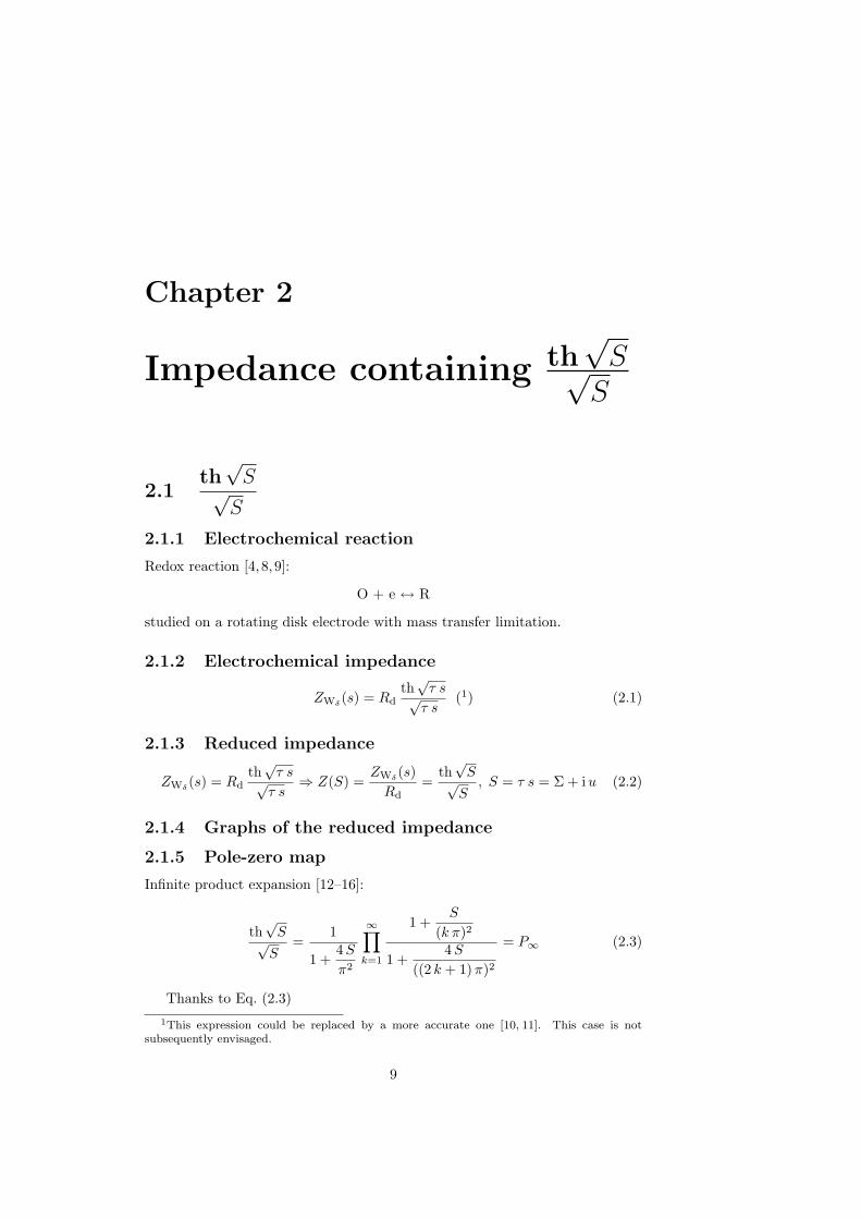
• infinity of interlaced real poles and zeros (Fig. 2.1).
sp = −14((2k + 1) π)2, k = 1 · · ·∞ (2.4)
sZ = −(k π)2, k = 1 · · ·∞ (2.5)
Figure 2.1: Pole-zero map ofth
√S√
s.
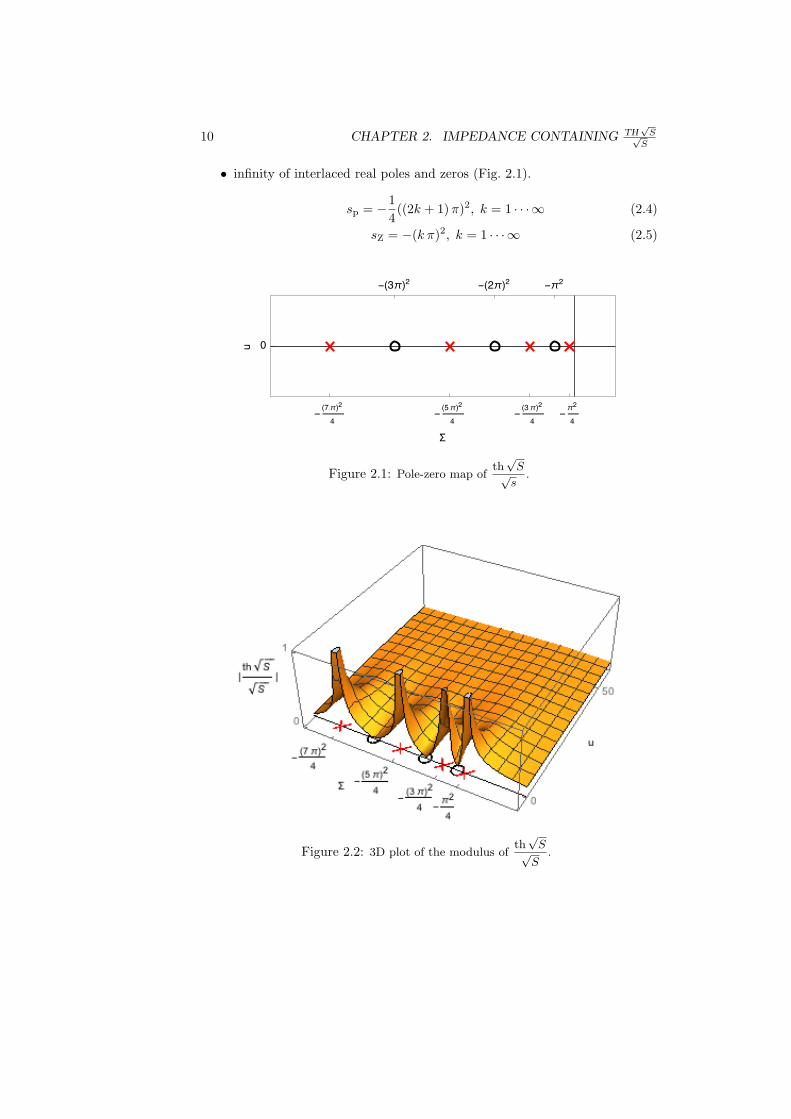
Figure 2.2: 3D plot of the modulus ofth
√S√
S.
2.2.
TH√
S√S
1 + α TH√
S√S
11
2.2
th√
S√S
1 + α th√
S√S
2.2.1 Electrochemical reaction
Corroding electrode with mass transfert limitation:
M → Mn+ + n e−
O2 + 4 e− + 4 H+ → 2 H2O
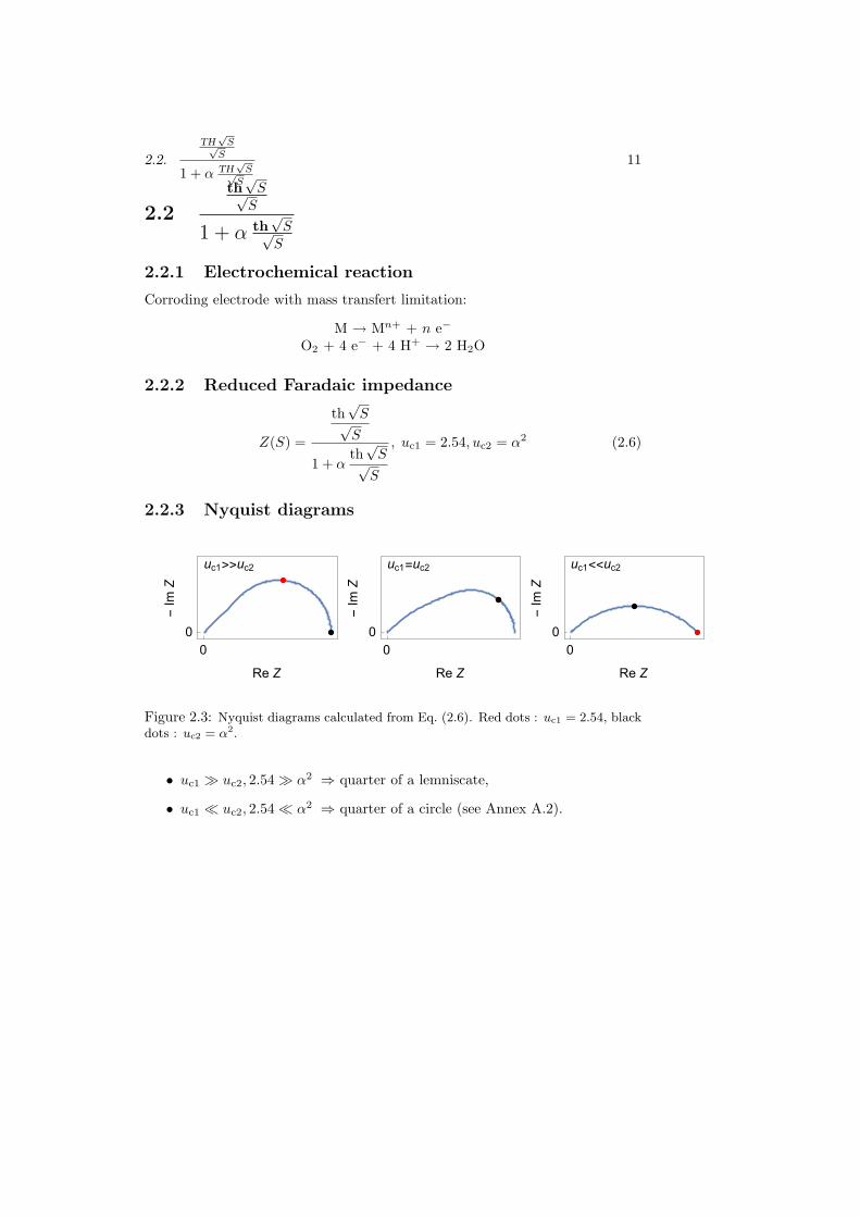
2.2.2 Reduced Faradaic impedance
Z(S) =
th√
S√S
1 + αth
√S√
S
, uc1 = 2.54, uc2 = α2 (2.6)
2.2.3 Nyquist diagrams
Figure 2.3: Nyquist diagrams calculated from Eq. (2.6). Red dots : uc1 = 2.54, blackdots : uc2 = α2.
• uc1 ≫ uc2, 2.54 ≫ α2 ⇒ quarter of a lemniscate,
• uc1 ≪ uc2, 2.54 ≪ α2 ⇒ quarter of a circle (see Annex A.2).
12 CHAPTER 2. IMPEDANCE CONTAINING TH√
S√S
2.3
(1 + α th
√S√
S
)th
√S√
S
1 + β th√
S√S
2.3.1 Electrochemical reaction
EE reaction [17]:
R ↔ X + eX ↔ O + e
studied on a rotating disk electrode with DR = DX = DO.
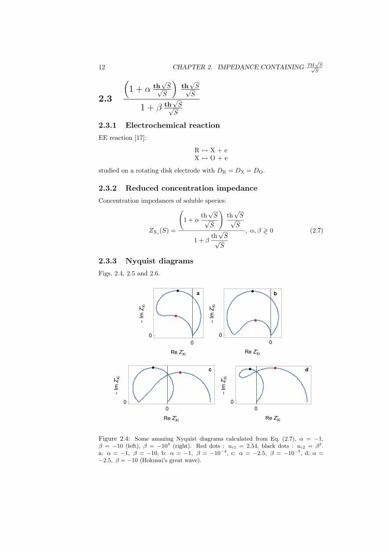
2.3.2 Reduced concentration impedance
Concentration impedances of soluble species:
ZXi(S) =
(1 + α
th√
S√S
)th
√S√
S
1 + βth
√S√
S
, α, β ≷ 0 (2.7)
2.3.3 Nyquist diagrams
Figs. 2.4, 2.5 and 2.6.
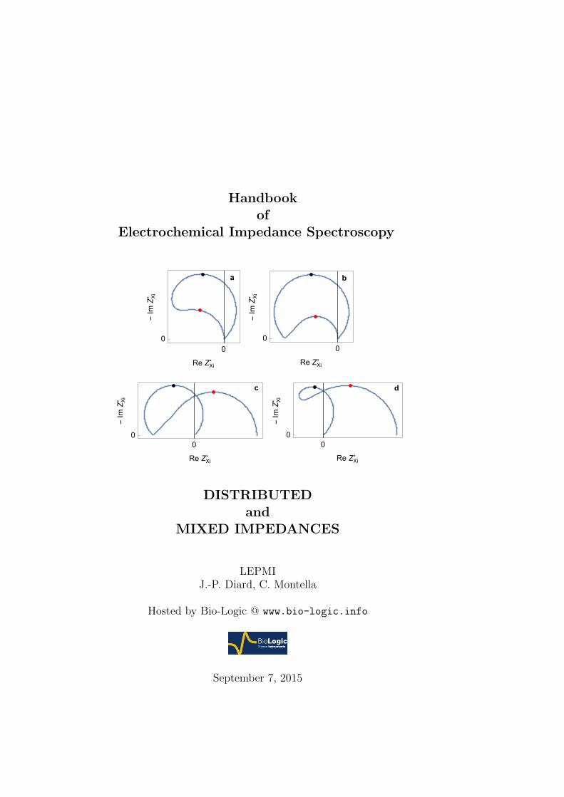
Figure 2.4: Some amazing Nyquist diagrams calculated from Eq. (2.7), α = −1,β = −10 (left), β = −104 (right). Red dots : uc1 = 2.54, black dots : uc2 = β2.a: α = −1, β = −10, b: α = −1, β = −10−4, c: α = −2.5, β = −10−5, d: α =−2.5, β = −10 (Hokusai’s great wave).
2.3.
(1 + α TH
√S√
S
)TH
√S√
S
1 + β TH√
S√S
13
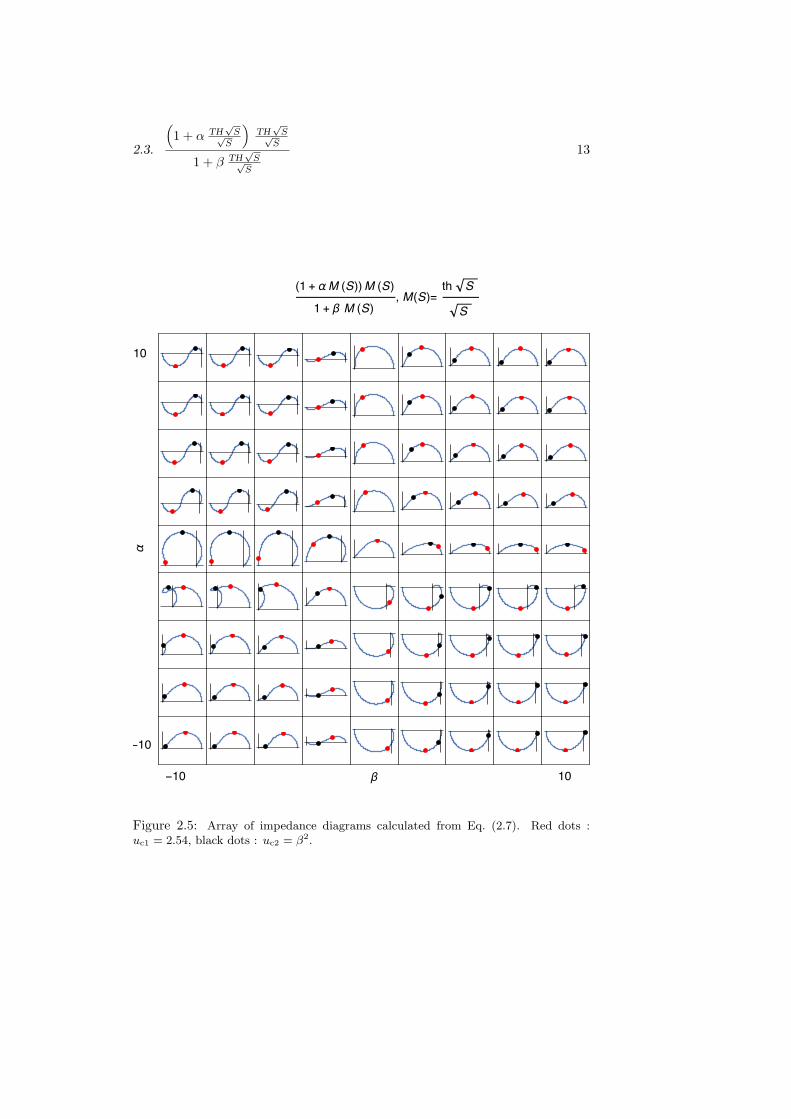
Figure 2.5: Array of impedance diagrams calculated from Eq. (2.7). Red dots :uc1 = 2.54, black dots : uc2 = β2.
14 CHAPTER 2. IMPEDANCE CONTAINING TH√
S√S
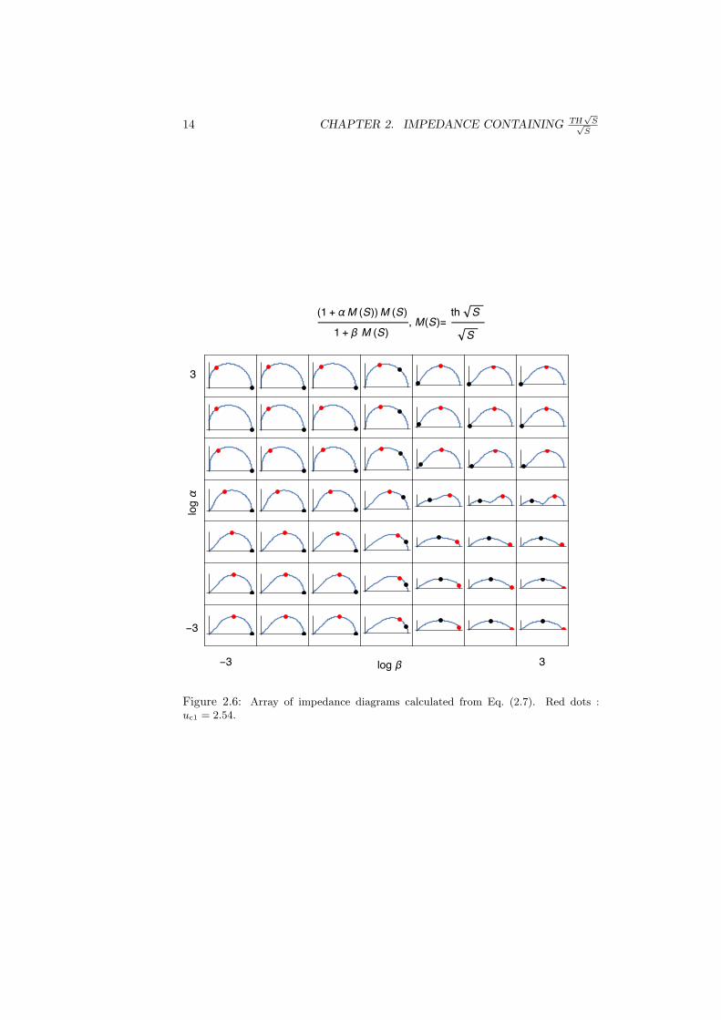
Figure 2.6: Array of impedance diagrams calculated from Eq. (2.7). Red dots :uc1 = 2.54.
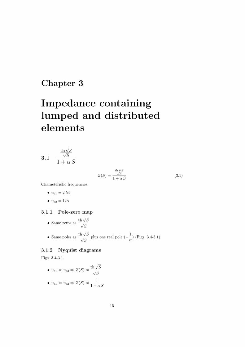
Chapter 3
Impedance containinglumped and distributedelements
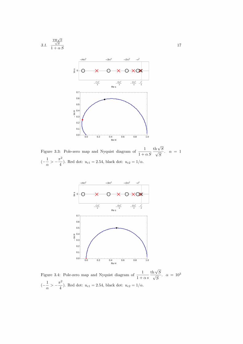
3.1
th√
S√S
1 + α S
Z(S) =th
√S√
S
1 + α S(3.1)
Characteristic frequencies:
• uc1 = 2.54
• uc2 = 1/α
3.1.1 Pole-zero map
• Same zeros asth
√S√
S
• Same poles asth
√S√
Splus one real pole (− 1
α) (Figs. 3.4-3.1).
3.1.2 Nyquist diagrams
Figs. 3.4-3.1.
• uc1 ≪ uc2 ⇒ Z(S) ≈ th√
S√S
• uc1 ≫ uc2 ⇒ Z(S) ≈ 11 + α S
15
16 CHAPTER 3. MIXED IMPEDANCE
-
Π2
4-
H3 ΠL2
4-
H5 ΠL2
4-
H7 ΠL2
4
0
-Π2
-H2ΠL2-H3ΠL2-H4ΠL2
Re sIm
s
0.0 0.2 0.4 0.6 0.8 1.00.0
0.1
0.2
0.3
0.4
0.5
0.6
0.7
Re H
-Im
H
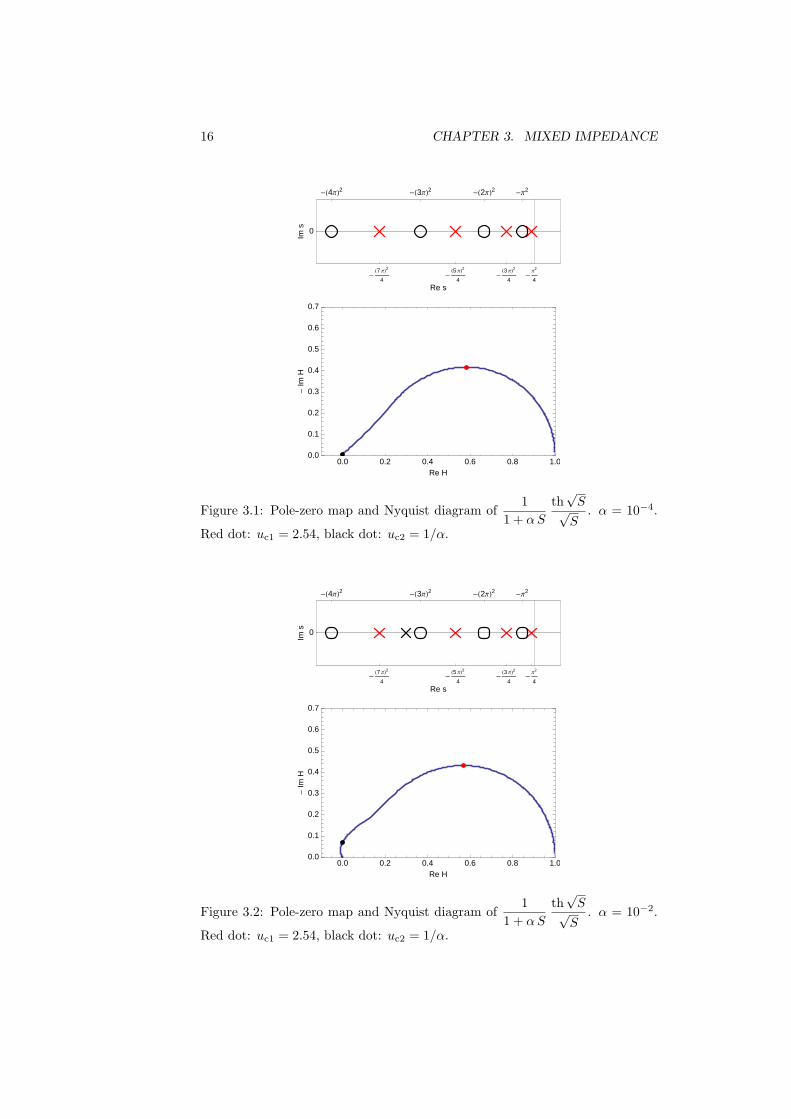
Figure 3.1: Pole-zero map and Nyquist diagram of1
1 + α S
th√
S√S
. α = 10−4.
Red dot: uc1 = 2.54, black dot: uc2 = 1/α.
-
Π2
4-
H3 ΠL2
4-
H5 ΠL2
4-
H7 ΠL2
4
0
-Π2
-H2ΠL2-H3ΠL2-H4ΠL2
Re s
Ims
0.0 0.2 0.4 0.6 0.8 1.00.0
0.1
0.2
0.3
0.4
0.5
0.6
0.7
Re H
-Im
H
Figure 3.2: Pole-zero map and Nyquist diagram of1
1 + α S
th√
S√S
. α = 10−2.
Red dot: uc1 = 2.54, black dot: uc2 = 1/α.
3.1.
TH√
S√S
1 + α S17
-
Π2
4-
H3 ΠL2
4-
H5 ΠL2
4-
H7 ΠL2
4
0
-Π2
-H2ΠL2-H3ΠL2-H4ΠL2
Re s
Ims
0.0 0.2 0.4 0.6 0.8 1.00.0
0.1
0.2
0.3
0.4
0.5
0.6
0.7
Re H
-Im
H
Figure 3.3: Pole-zero map and Nyquist diagram of1
1 + α S
th√
S√S
. α = 1
(− 1α
> −π2
4). Red dot: uc1 = 2.54, black dot: uc2 = 1/α.
-
Π2
4-
H3 ΠL2
4-
H5 ΠL2
4-
H7 ΠL2
4
0
-Π2
-H2ΠL2-H3ΠL2-H4ΠL2
Re s
Ims
0.0 0.2 0.4 0.6 0.8 1.00.0
0.1
0.2
0.3
0.4
0.5
0.6
0.7
Re H
-Im
H
Figure 3.4: Pole-zero map and Nyquist diagram of1
1 + α s
th√
S√S
. α = 103
(− 1α
> −π2
4). Red dot: uc1 = 2.54, black dot: uc2 = 1/α.
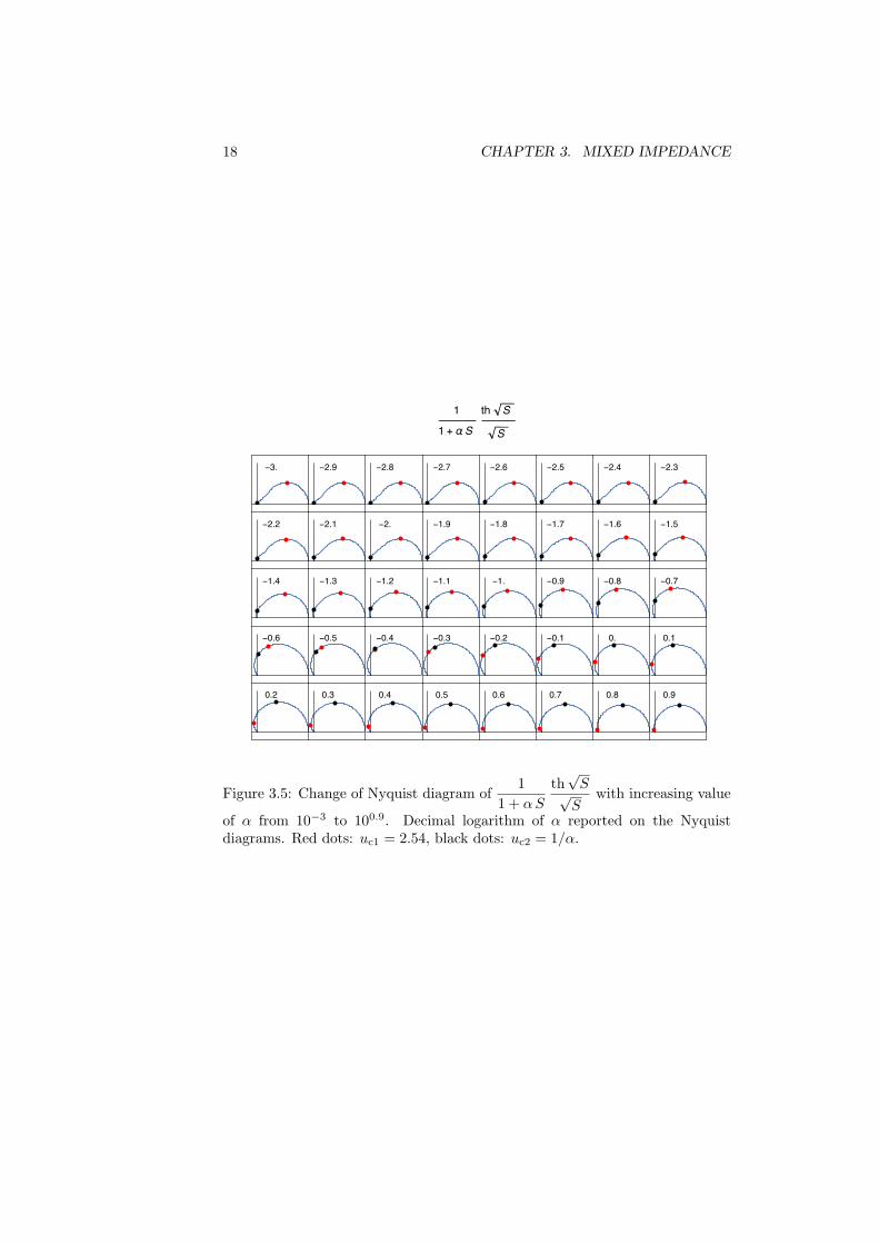
18 CHAPTER 3. MIXED IMPEDANCE
Figure 3.5: Change of Nyquist diagram of1
1 + α S
th√
S√S
with increasing value
of α from 10−3 to 100.9. Decimal logarithm of α reported on the Nyquistdiagrams. Red dots: uc1 = 2.54, black dots: uc2 = 1/α.
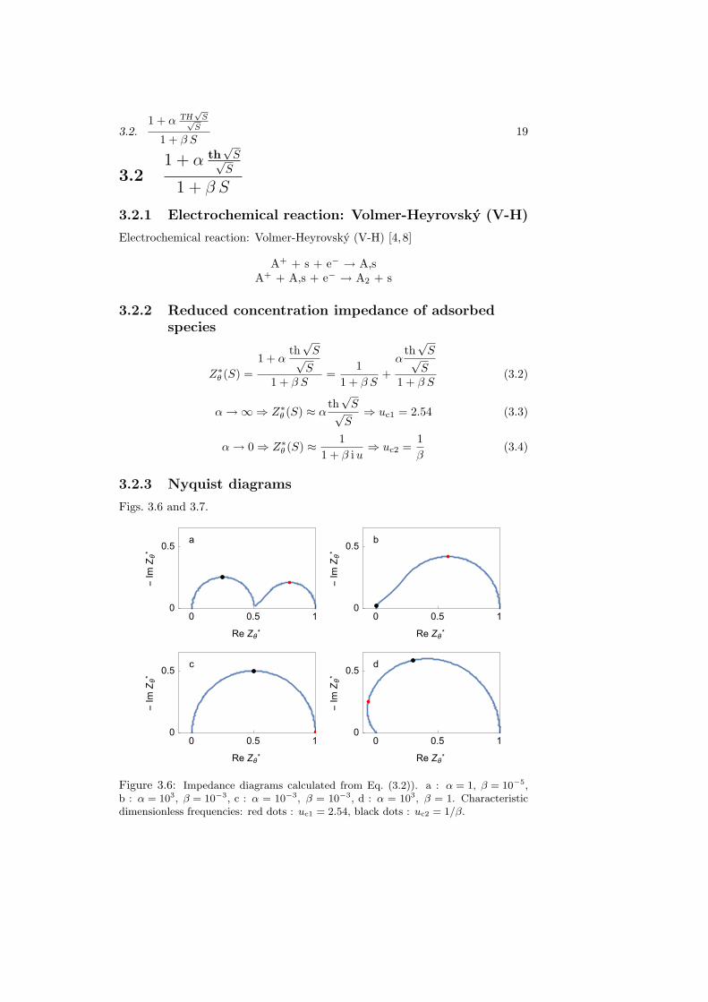
3.2.1 + α TH
√S√
S
1 + β S19
3.21 + α th
√S√
S
1 + β S
3.2.1 Electrochemical reaction: Volmer-Heyrovsky (V-H)
Electrochemical reaction: Volmer-Heyrovsky (V-H) [4,8]
A+ + s + e− → A,sA+ + A,s + e− → A2 + s
3.2.2 Reduced concentration impedance of adsorbedspecies
Z∗θ (S) =
1 + αth
√S√
S1 + β S
=1
1 + β S+
αth
√S√
S1 + β S
(3.2)
α → ∞ ⇒ Z∗θ (S) ≈ α
th√
S√S
⇒ uc1 = 2.54 (3.3)
α → 0 ⇒ Z∗θ (S) ≈ 1
1 + β iu⇒ uc2 =
1β
(3.4)
3.2.3 Nyquist diagrams
Figs. 3.6 and 3.7.
Figure 3.6: Impedance diagrams calculated from Eq. (3.2)). a : α = 1, β = 10−5,b : α = 103, β = 10−3, c : α = 10−3, β = 10−3, d : α = 103, β = 1. Characteristicdimensionless frequencies: red dots : uc1 = 2.54, black dots : uc2 = 1/β.
20 CHAPTER 3. MIXED IMPEDANCE
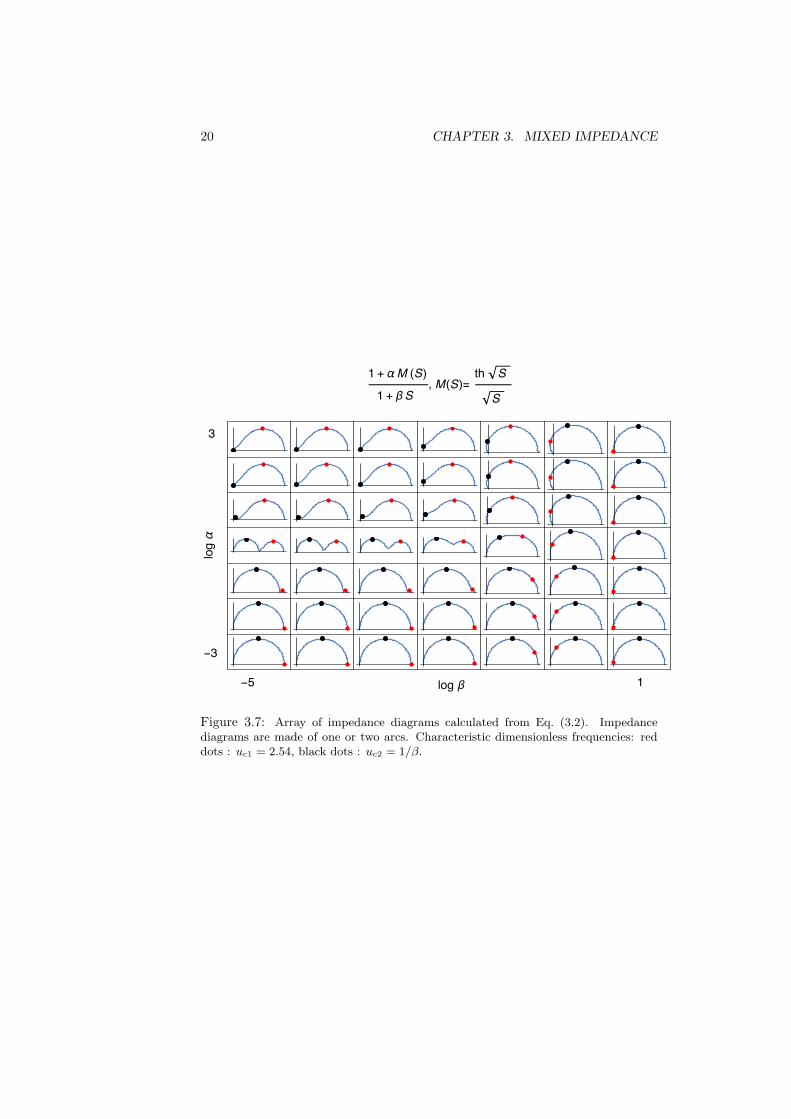
Figure 3.7: Array of impedance diagrams calculated from Eq. (3.2). Impedancediagrams are made of one or two arcs. Characteristic dimensionless frequencies: reddots : uc1 = 2.54, black dots : uc2 = 1/β.
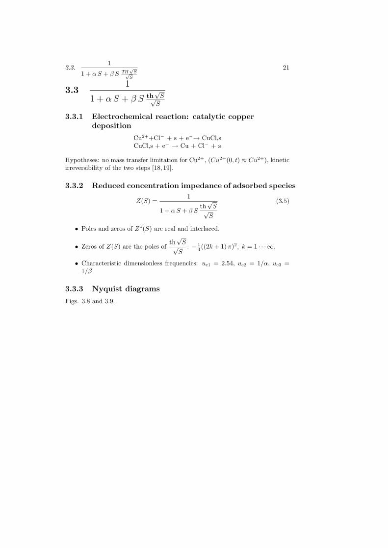
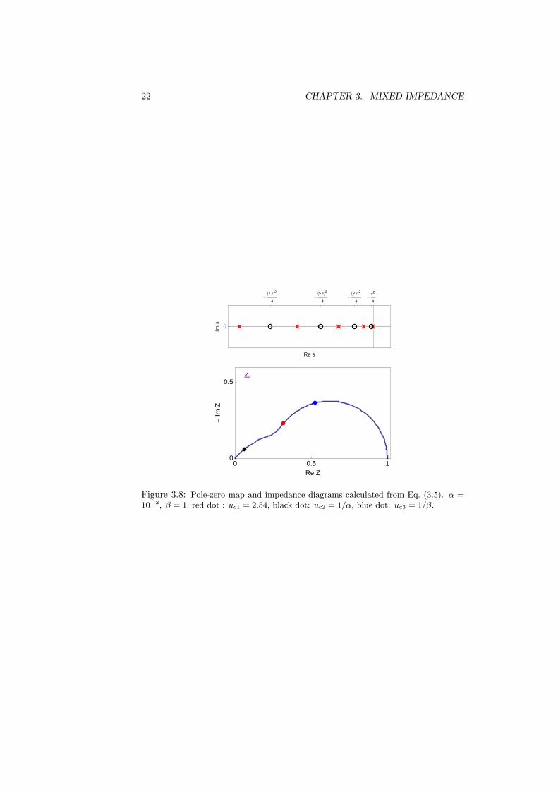
3.3.1
1 + α S + β S TH√
S√S
21
3.31
1 + α S + β S th√
S√S
3.3.1 Electrochemical reaction: catalytic copperdeposition
Cu2++Cl− + s + e−→ CuCl,sCuCl,s + e− → Cu + Cl− + s
Hypotheses: no mass transfer limitation for Cu2+, (Cu2+(0, t) ≈ Cu2+), kineticirreversibility of the two steps [18,19].
3.3.2 Reduced concentration impedance of adsorbed species
Z(S) =1
1 + α S + β Sth
√S√
S
(3.5)
• Poles and zeros of Z∗(S) are real and interlaced.
• Zeros of Z(S) are the poles ofth
√S√
S: − 1
4 ((2k + 1) π)2, k = 1 · · ·∞.
• Characteristic dimensionless frequencies: uc1 = 2.54, uc2 = 1/α, uc3 =1/β
3.3.3 Nyquist diagrams
Figs. 3.8 and 3.9.
22 CHAPTER 3. MIXED IMPEDANCE
0
-Π
2
4-I3 ΠM2
4-I5 ΠM2
4-I7 ΠM2
4
Re s
Ims
0 0.5 10
0.5
Re Z
-Im
Z
ZΘ
Figure 3.8: Pole-zero map and impedance diagrams calculated from Eq. (3.5). α =10−2, β = 1, red dot : uc1 = 2.54, black dot: uc2 = 1/α, blue dot: uc3 = 1/β.
3.3.1
1 + α S + β S TH√
S√S
23
Figure 3.9: Graphics array representation of the impedance diagram, calculatedform Eq. (3.5) and plotted using the Nyquist representation (orthonormal scales)for catalytic copper deposition. Characteristic dimensionless frequencies: red dots :uc1 = 2.54, black dots: uc2 = 1/α, blue dots: uc3 = 1/β.
24 CHAPTER 3. MIXED IMPEDANCE
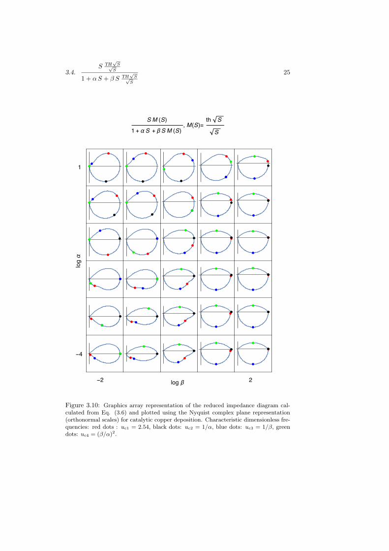
3.4S th
√S√
S
1 + α S + β S th√
S√S
3.4.1 Electrochemical reaction: catalytic copperdeposition
Cu2++Cl− + s + e−→ CuCl,sCuCl,s + e− → Cu + Cl− + s
Hypotheses: no mass transfer limitation for Cu2+, (Cu2+(0, t) ≈ Cu2+), kineticirreversibility of the two steps [19].
3.4.2 Reduced concentration impedance of solublespecies Cl−
Z(S) =S
th√
S√S
1 + α S + β Sth
√S√
S
(3.6)
3.4.3 Nyquist diagrams
• Poles and zeros of Z(S) are real.
• Zeros of Z(S) are the zeros ofth
√S√
S(SZ = −(k π)2, k = 1 · · ·∞) plus
one zero at the origine of the complex plane (derivator).
• Characteristic dimensionless frequencies: uc1 = 2.54, uc2 = 1/α, uc3 =1/β, uc4 = (β/α)2.
Fig. 3.10.
3.4.S TH
√S√
S
1 + α S + β S TH√
S√S
25
Figure 3.10: Graphics array representation of the reduced impedance diagram cal-culated from Eq. (3.6) and plotted using the Nyquist complex plane representation(orthonormal scales) for catalytic copper deposition. Characteristic dimensionless fre-quencies: red dots : uc1 = 2.54, black dots: uc2 = 1/α, blue dots: uc3 = 1/β, greendots: uc4 = (β/α)2.
26 CHAPTER 3. MIXED IMPEDANCE
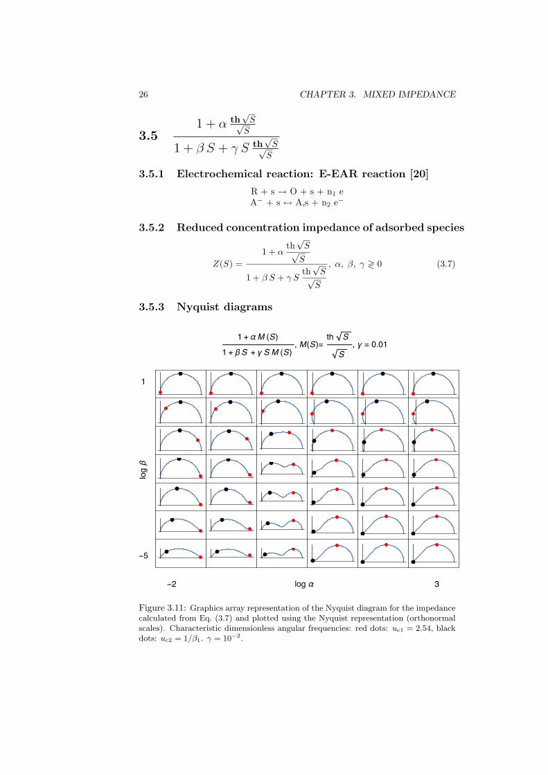
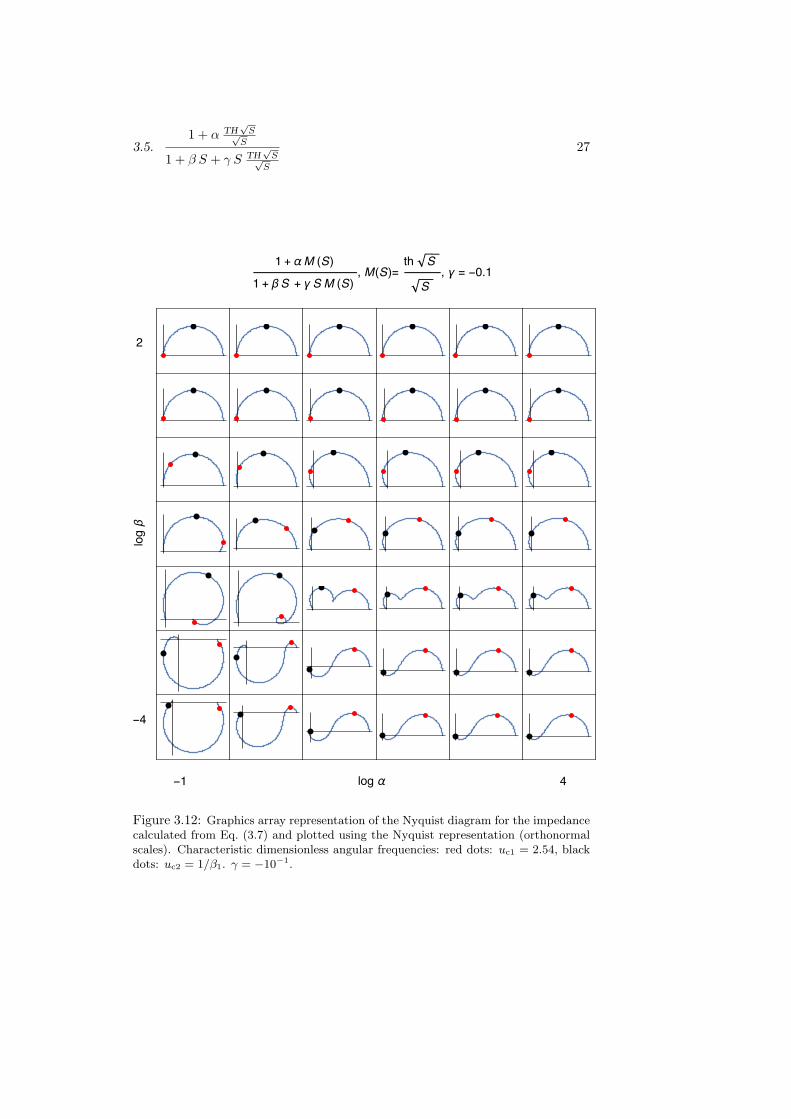
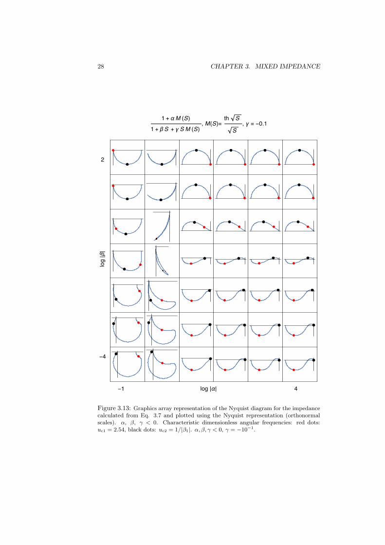
3.51 + α th
√S√
S
1 + β S + γ S th√
S√S
3.5.1 Electrochemical reaction: E-EAR reaction [20]
R + s → O + s + n1 eA− + s ↔ A,s + n2 e−
3.5.2 Reduced concentration impedance of adsorbed species
Z(S) =1 + α
th√
S√S
1 + β S + γ Sth
√S√
S
, α, β, γ ≷ 0 (3.7)
3.5.3 Nyquist diagrams
Figure 3.11: Graphics array representation of the Nyquist diagram for the impedancecalculated from Eq. (3.7) and plotted using the Nyquist representation (orthonormalscales). Characteristic dimensionless angular frequencies: red dots: uc1 = 2.54, blackdots: uc2 = 1/β1. γ = 10−2.
3.5.1 + α TH
√S√
S
1 + β S + γ S TH√
S√S
27
Figure 3.12: Graphics array representation of the Nyquist diagram for the impedancecalculated from Eq. (3.7) and plotted using the Nyquist representation (orthonormalscales). Characteristic dimensionless angular frequencies: red dots: uc1 = 2.54, blackdots: uc2 = 1/β1. γ = −10−1.
28 CHAPTER 3. MIXED IMPEDANCE
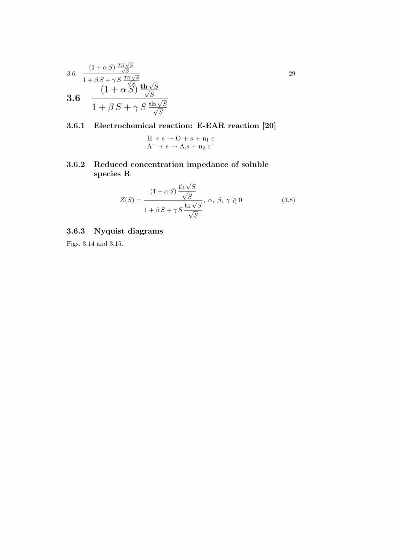
Figure 3.13: Graphics array representation of the Nyquist diagram for the impedancecalculated from Eq. 3.7 and plotted using the Nyquist representation (orthonormalscales). α, β, γ < 0. Characteristic dimensionless angular frequencies: red dots:uc1 = 2.54, black dots: uc2 = 1/|β1|. α, β, γ < 0, γ = −10−1.
3.6.(1 + α S) TH
√S√
S
1 + β S + γ S TH√
S√S
29
3.6(1 + α S) th
√S√
S
1 + β S + γ S th√
S√S
3.6.1 Electrochemical reaction: E-EAR reaction [20]
R + s → O + s + n1 eA− + s → A,s + n2 e−
3.6.2 Reduced concentration impedance of solublespecies R
Z(S) =(1 + α S)
th√
S√S
1 + β S + γ Sth
√S√
S
, α, β, γ ≷ 0 (3.8)
3.6.3 Nyquist diagrams
Figs. 3.14 and 3.15.
30 CHAPTER 3. MIXED IMPEDANCE
Figure 3.14: Graphics array representation of the Nyquist diagram for the impedancecalculated from Eq. (3.8) and plotted using the Nyquist representation (orthonormalscales). Characteristic dimensionless angular frequencies: red dots: uc1 = 2.54, blackdots: uc2 = 1/β. γ = 10−3.
3.6.(1 + α S) TH
√S√
S
1 + β S + γ S TH√
S√S
31
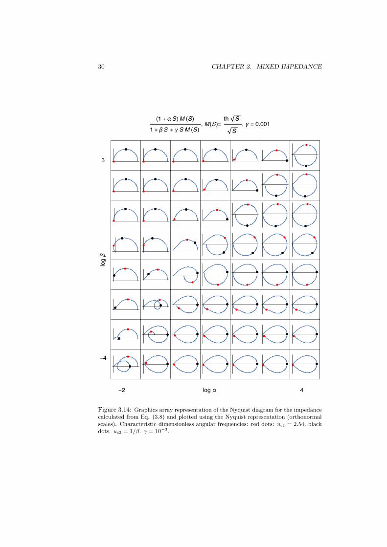
Figure 3.15: Graphics array representation of the Nyquist diagram for the impedancecalculated from Eq. (3.8) and plotted using the Nyquist representation (orthonormalscales). α, β, γ < 0. Characteristic dimensionless angular frequencies: red dots:uc1 = 2.54, black dots: uc2 = 1/|β|. γ = 10−3.

32 CHAPTER 3. MIXED IMPEDANCE
Appendix A
Some rational fractions in√S
A.1 Introduction
The use of a rational fraction in√
S
Z(√
S) =∑N
m=0 bm(√
S)m∑Pp=0 ap(
√S)p
(A.1)
has been proposed by Pintelon et al. [21, 22]. Some rational fraction in√
S arestudied below.
A.21
1 +√
S
H(u) =1
1 +√
iu(A.2)
Re H(u) =√
2√
u + 22(u +
√2√
u + 1) , Im H(u) = −
√u√
2(u +
√2√
u + 1) (A.3)
|H(u) − (1/2 + i/2)| =√
(Re H(u) − 1/2)2 + (Im H(u) − 1/2)2 =√
22
⇒ circle, radius =√
22
(A.4)
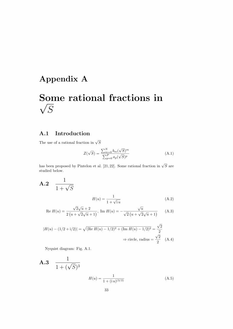
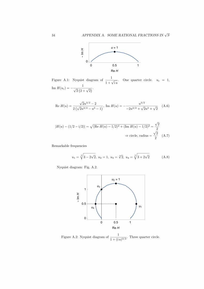
Nyquist diagram: Fig. A.1.
A.31
1 + (√
S)3
H(u) =1
1 + (iu)(3/2)(A.5)
33
34 APPENDIX A. SOME RATIONAL FRACTIONS IN√
S
Figure A.1: Nyquist diagram of1
1 +√
iu. One quarter circle. uc = 1,
Im H(uc) = − 1√2(2 +
√2) .
Re H(u) =√
2u3/2 − 22(√
2u3/2 − u3 − 1) , Im H(u) = − u3/2
−2u3/2 +√
2u3 +√
2(A.6)
|H(u) − (1/2 − i/2)| =√
(Re H(u) − 1/2)2 + (Im H(u) − 1/2)2 =√
22
⇒ circle, radius =√
22
(A.7)
Remarkable frequencies
u1 =3√
3 − 2√
2, u2 = 1, u3 = 3√
2, u4 =3√
3 + 2√
2 (A.8)
Nyquist diagram: Fig. A.2.
Figure A.2: Nyquist diagram of1
1 + (iu)3/2. Three quarter circle.
A.4.1 + (
√S)2√
S (1 + α(√
S)2)35
A.41 + (
√S)2
√S (1 + α(
√S)2)
H(u) =1 + (
√iu)2√
iu (1 + α (√
iu)2)(A.9)
Re H(u) =u(α(u − 1) + 1) + 1√
2√
u (α2u2 + 1), Im H(u) =
−u(αu + α − 1) − 1√2√
u (α2u2 + 1)(A.10)
Three different limiting cases
• α ≪ 1, Nyquist and Bode diagrams: Fig. A.3
u1 = uIm H=0 =−√
α2 − 6α + 1 − α + 12α
≈ 1 (A.11)
u2 = uIm H=0 =+√
α2 − 6α + 1 − α + 12α
≈ 1α
(A.12)
• α = 1, H(u) =1√iu
• α ≫ 1, Nyquist diagram: Fig. A.4
u1 = uReH=0 =−√
α2 − 6α + 1 + α − 12α
≈ 1α
(A.13)
u2 = uReH=0 =√
α2 − 6α + 1 + α − 12α
≈ 1 (A.14)
A.51 − (
√S)2
√S (1 − α(
√S)2)
H(u) =1 − (
√iu)2√
iu (1 − α (√
iu)2)(A.15)
Re H(u) =u(α + αu − 1) + 1√
2√
u (α2u2 + 1), Im H(u) =
u(α + α(−u) − 1) − 1√2√
u (α2u2 + 1)(A.16)
Three different limiting cases
• α ≪ 1, Nyquist diagram: Fig. A.5
u1 = uRe H=0 =−√
α2 − 6α + 1 − α + 12α
≈ 1 (A.17)
u2 = uRe H=0 =√
α2 − 6α + 1 − α + 12α
≈ 1α
(A.18)
• α = 1, H(u) =1√iu
• α ≫ 1.
36 APPENDIX A. SOME RATIONAL FRACTIONS IN√
S
Figure A.3: Nyquist and Bode (modulus) diagram of1 + (
√iu)2√
iu (1 + α (√
iu)2).
a ≪ 1. Red dot: u2 =≈ 1/α, black dot: u1 = 0 ≈ 1.
Figure A.4: Nyquist and Bode (modulus) diagram of1 + (
√iu)2√
iu (1 + α (√
iu)2).
a ≫ 1. Red dot: uIm H=0 ≈ 1/α, black dot: uIm H=0 ≈ 1.
A.5.1 − (
√S)2√
S (1 − α(√
S)2)37
Figure A.5: Nyquist and Bode (modulus) diagram of1 − (
√iu)2√
iu (1 − α (√
iu)2).
a ≪ 1. Red dot: u2 =≈ 1/α, black dot: u1 = 0 ≈ 1.

38 APPENDIX A. SOME RATIONAL FRACTIONS IN√
S
Appendix B
Impedance structure ofreactions involving bothadsorbed and solublespecies
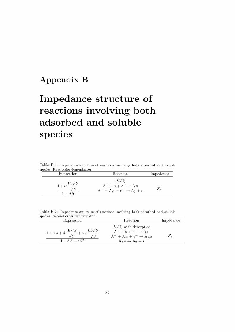
Table B.1: Impedance structure of reactions involving both adsorbed and solublespecies. First order denominator.
Expression Reaction Impedance
1 + αth
√S√
S1 + β S
(V-H)A+ + s + e− → A,s
A+ + A,s + e− → A2 + s Zθ
Table B.2: Impedance structure of reactions involving both adsorbed and solublespecies. Second order denominator.
Expression Reaction Impedance
1 + α s + βth
√S√
S+ γ s
th√
S√S
1 + δ S + ϵ S2
(V-H) with desorptionA+ + s + e− → A,s
A+ + A,s + e− → A2,sA2,s → A2 + s
Zθ
39
40APPENDIX B. REACTIONS INVOLVING ADSORBED AND SOLUBLE SPECIES
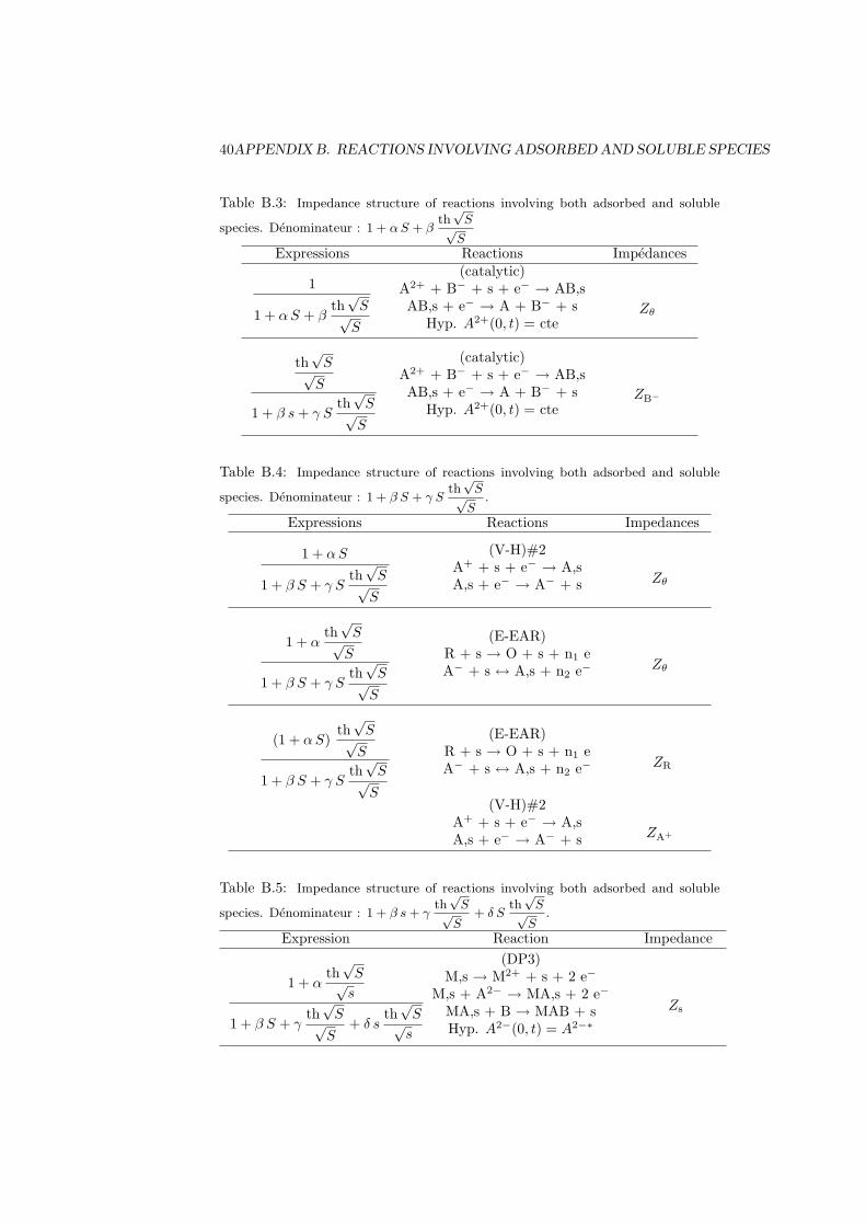
Table B.3: Impedance structure of reactions involving both adsorbed and soluble
species. Denominateur : 1 + α S + βth
√S√
SExpressions Reactions Impedances
1
1 + α S + βth
√S√
S
(catalytic)A2+ + B− + s + e− → AB,sAB,s + e− → A + B− + s
Hyp. A2+(0, t) = cteZθ
th√
S√S
1 + β s + γ Sth
√S√
S
(catalytic)A2+ + B− + s + e− → AB,sAB,s + e− → A + B− + s
Hyp. A2+(0, t) = cteZB−
Table B.4: Impedance structure of reactions involving both adsorbed and soluble
species. Denominateur : 1 + β S + γ Sth
√S√
S.
Expressions Reactions Impedances
1 + α S
1 + β S + γ Sth
√S√
S
(V-H)#2A+ + s + e− → A,sA,s + e− → A− + s Zθ
1 + αth
√S√
S
1 + β S + γ Sth
√S√
S
(E-EAR)R + s → O + s + n1 eA− + s ↔ A,s + n2 e− Zθ
(1 + α S)th
√S√
S
1 + β S + γ Sth
√S√
S
(E-EAR)R + s → O + s + n1 eA− + s ↔ A,s + n2 e− ZR
(V-H)#2A+ + s + e− → A,sA,s + e− → A− + s ZA+
Table B.5: Impedance structure of reactions involving both adsorbed and soluble
species. Denominateur : 1 + β s + γth
√S√
S+ δ S
th√
S√S
.
Expression Reaction Impedance
1 + αth
√S√
s
1 + β S + γth
√S√
S+ δ s
th√
S√s
(DP3)M,s → M2+ + s + 2 e−
M,s + A2− → MA,s + 2 e−
MA,s + B → MAB + sHyp. A2−(0, t) = A2−∗
Zs
Bibliography
[1] G. C. Temes and J. W. LaPatra. Introduction to Circuits Synthesis and Design.McGraw-Hill, New-York, 1977.
[2] R. Curtain and K. Morris. Transfer functions of distributed parameter systems:A tutorial. Automatica, 45:1101 – 1116, 2009.
[3] J.-P. Diard, B. Le Gorrec, and C. Montella. Cinetique electrochimique. Hermann,Paris, 1996.
[4] Handbook of EIS - Faradaic impedance library.www.bio-logic.info/potentiostat-electrochemistry-ec-lab/apps-literature/eis-literature/hanbook-of-eis/.
[5] Handbook of EIS - Electrical circuits containing CPEs.www.bio-logic.info/potentiostat-electrochemistry-ec-lab/apps-literature/eis-literature/hanbook-of-eis/.
[6] Handbook of EIS - Diffusion impedances.www.bio-logic.info/potentiostat-electrochemistry-ec-lab/apps-literature/eis-literature/hanbook-of-eis/.
[7] J. E. Randles. Kinetics of rapid electrode reactions. Discuss. Faraday Soc., 1:11,1947.
[8] Interactive equivalent circuit library.http://www.bio-logic.info/potentiostat-electrochemistry-ec-lab/apps-literature/interactive-eis/interactive-faradaic-impedance-library/.
[9] J.-P. Diard and C. Montella. Impedance of a Redox Reaction (E) at a RotatingDisk Electrode (RDE). Wolfram Demonstrations Project, 2010.http://demonstrations.wolfram.com/ImpedanceOfARedoxReactionEAtARota-tingDiskElectrodeRDE/.
[10] R. Michel and C. Montella. Diffusion-convection impedance using an efficient an-alytical approximation of the mass transfer function for a rotating disk. J. Elec-troanal. Chem, 736:139 – 146, 2015.
[11] J.-P. Diard and C. Montella. Re-examination of the diffusion-convectionimpedance for a uniformly accessible rotating disk. computation and accuracy.J. Electroanal. Chem., 742:37 – 46, 2015.
[12] J. Crank. The Mathematics of Diffusion. Clarendon Press, Oxford, 2 edition,1975.
[13] F. Berthier, J.-P. Diard, B. Le Gorrec, and C. Montella. La resistance de transfertd’electrons d’une reaction electrochimique peut-elle etre negative ? C. R. Acad.Sci. Paris, Serie II b, 325:21–26, 1997.
[14] F. Berthier, J.-P. Diard, and C. Montella. Developpement en produits infinisdes operateurs de transport de matiere. Application en spectroscopie d’impedanceelectrochimique et en voltamperometrie lineaire. In C. Gabrielli, editor, Proceeding
41
42 BIBLIOGRAPHY
of the 11th Forum sur les Impedances Electrochimiques, pages 189–196, Paris,December 1998.
[15] F. Berthier, J.-P. Diard, and C. Montella. Hopf bifurcation and sign of the transferresistance. Electrochim. Acta, 44:2397–2404, 1999.
[16] F. Berthier, J.-P. Diard, and C. Montella. Numerical solution of coupled systemsof ordinary and partial differential equations. Application to the study of electro-chemical insertion reaction by linear sweep voltammetry. J. Electroanal. Chem.,502:126–131, 2001.
[17] J.-P. Diard and C. Montella. Non-intuitive features of equivalent circuits foranalysis of EIS data. The example of EE reaction. J. Electroanal. Chem., 735:99– 110, 2014.
[18] C. Gabrielli, P. Mocoteguy, H. Perrot, and R. Wiart. Mechanism of copper depo-sition in a sulphate bath containing chlorides. J. Electroanal. Chem., 572:367–375,2004.
[19] J.-P. Diard and C. Montella. Unusual concentration impedance for catalytic cop-per deposition. J. Electroanal. Chem., 590:126–137, 2006.
[20] M.B. Molina Concha, M. Chatenet, C. Montella, and J.-P. Diard. A Faradaicimpedance study of E-EAR reaction. J. Electroanal. Chem, 696:24 – 37, 2013.
[21] R. Pintelon and J. Schoukens. System Identification. A frequency domain ap-proach. IEEE Press, Piscataway, USA, 2001.
[22] L. Pauwels, W. Simons, A. Hubin, J. Schoukens, and R. Pintelon. Key issues forreproducible impedance measurements and their well-founded error analysis in asilver electrodeposition system. Electrochim. Acta, 47:2135 – 2141, 2002.