Handbook of Robotics

Chapter 1: Kinematics

Ken WaldronDepartment of Mechanical Engineering

Stanford UniversityStanford, CA 94305, USA

Jim SchmiedelerDepartment of Mechanical Engineering

The Ohio State UniversityColumbus, OH 43210, USA

September 15, 2005

Contents

1 Kinematics 11.1 Introduction . . . . . . . . . . . . . . . . . . . . . . . . . . . . . . . . . . . . . . . . . . . . . . . . . . 11.2 Position and Orientation Representation . . . . . . . . . . . . . . . . . . . . . . . . . . . . . . . . . . 2

1.2.1 Representation of Position . . . . . . . . . . . . . . . . . . . . . . . . . . . . . . . . . . . . . . 21.2.2 Representation of Orientation . . . . . . . . . . . . . . . . . . . . . . . . . . . . . . . . . . . . 2

Rotation Matrices . . . . . . . . . . . . . . . . . . . . . . . . . . . . . . . . . . . . . . . . . . 2Euler Angles . . . . . . . . . . . . . . . . . . . . . . . . . . . . . . . . . . . . . . . . . . . . . 3Fixed Angles . . . . . . . . . . . . . . . . . . . . . . . . . . . . . . . . . . . . . . . . . . . . . 3Angle-Axis . . . . . . . . . . . . . . . . . . . . . . . . . . . . . . . . . . . . . . . . . . . . . . 4Quaternions . . . . . . . . . . . . . . . . . . . . . . . . . . . . . . . . . . . . . . . . . . . . . . 4

1.2.3 Homogeneous Transformations . . . . . . . . . . . . . . . . . . . . . . . . . . . . . . . . . . . 51.2.4 Screw Transformations . . . . . . . . . . . . . . . . . . . . . . . . . . . . . . . . . . . . . . . . 51.2.5 Plucker Coordinates . . . . . . . . . . . . . . . . . . . . . . . . . . . . . . . . . . . . . . . . . 6

1.3 Joint Kinematics . . . . . . . . . . . . . . . . . . . . . . . . . . . . . . . . . . . . . . . . . . . . . . . 61.3.1 Revolute . . . . . . . . . . . . . . . . . . . . . . . . . . . . . . . . . . . . . . . . . . . . . . . . 71.3.2 Prismatic . . . . . . . . . . . . . . . . . . . . . . . . . . . . . . . . . . . . . . . . . . . . . . . 71.3.3 Helical . . . . . . . . . . . . . . . . . . . . . . . . . . . . . . . . . . . . . . . . . . . . . . . . . 81.3.4 Cylindrical . . . . . . . . . . . . . . . . . . . . . . . . . . . . . . . . . . . . . . . . . . . . . . 81.3.5 Spherical . . . . . . . . . . . . . . . . . . . . . . . . . . . . . . . . . . . . . . . . . . . . . . . 81.3.6 Planar . . . . . . . . . . . . . . . . . . . . . . . . . . . . . . . . . . . . . . . . . . . . . . . . . 91.3.7 Universal . . . . . . . . . . . . . . . . . . . . . . . . . . . . . . . . . . . . . . . . . . . . . . . 91.3.8 Rolling Contact . . . . . . . . . . . . . . . . . . . . . . . . . . . . . . . . . . . . . . . . . . . . 91.3.9 Holonomic and Non-Holonomic Constraints . . . . . . . . . . . . . . . . . . . . . . . . . . . . 91.3.10 Generalized Coordinates . . . . . . . . . . . . . . . . . . . . . . . . . . . . . . . . . . . . . . . 9

1.4 Workspace . . . . . . . . . . . . . . . . . . . . . . . . . . . . . . . . . . . . . . . . . . . . . . . . . . . 91.5 Geometric Representation . . . . . . . . . . . . . . . . . . . . . . . . . . . . . . . . . . . . . . . . . . 101.6 Forward Kinematics . . . . . . . . . . . . . . . . . . . . . . . . . . . . . . . . . . . . . . . . . . . . . 121.7 Inverse Kinematics . . . . . . . . . . . . . . . . . . . . . . . . . . . . . . . . . . . . . . . . . . . . . . 12

1.7.1 Closed-Form Solutions . . . . . . . . . . . . . . . . . . . . . . . . . . . . . . . . . . . . . . . . 13Algebraic Methods . . . . . . . . . . . . . . . . . . . . . . . . . . . . . . . . . . . . . . . . . . 13Geometric Methods . . . . . . . . . . . . . . . . . . . . . . . . . . . . . . . . . . . . . . . . . 13

1.7.2 Numerical Methods . . . . . . . . . . . . . . . . . . . . . . . . . . . . . . . . . . . . . . . . . 14Symbolic Elimination Methods . . . . . . . . . . . . . . . . . . . . . . . . . . . . . . . . . . . 14Continuation Methods . . . . . . . . . . . . . . . . . . . . . . . . . . . . . . . . . . . . . . . . 14Iterative Methods . . . . . . . . . . . . . . . . . . . . . . . . . . . . . . . . . . . . . . . . . . 14

1.8 Forward Instantaneous Kinematics . . . . . . . . . . . . . . . . . . . . . . . . . . . . . . . . . . . . . 141.8.1 Jacobian . . . . . . . . . . . . . . . . . . . . . . . . . . . . . . . . . . . . . . . . . . . . . . . . 15

1.9 Inverse Instantaneous Kinematics . . . . . . . . . . . . . . . . . . . . . . . . . . . . . . . . . . . . . . 15

i

CONTENTS ii

1.9.1 Inverse Jacobian . . . . . . . . . . . . . . . . . . . . . . . . . . . . . . . . . . . . . . . . . . . 151.10 Static Wrench Transmission . . . . . . . . . . . . . . . . . . . . . . . . . . . . . . . . . . . . . . . . . 161.11 Conclusions and Further Reading . . . . . . . . . . . . . . . . . . . . . . . . . . . . . . . . . . . . . . 16

List of Figures

1.1 place holder . . . . . . . . . . . . . . . . . . . . . . . . . . . . . . . . . . . . . . . . . . . . . . . . . . 111.2 Example Six-Degree-of-Freedom Serial Chain Manipulator. . . . . . . . . . . . . . . . . . . . . . . . 11

iii

List of Tables

1.1 Equivalent rotation matrices for various representations of orientation. . . . . . . . . . . . . . . . . . 31.2 Conversions from a rotation matrix to various representations of orientation. . . . . . . . . . . . . . 41.3 Conversions from angle-axis to unit quaternion representations of orientation and vice versa. . . . . 41.4 Conversions from a screw transformation to a homogeneous transformation and vice versa. . . . . . 61.5 Tabulated Geometric Parameters for Example Serial Chain Manipulator. . . . . . . . . . . . . . . . . 111.6 Forward Kinematics of the Example Serial Chain Manipulator in Figure 1.2. . . . . . . . . . . . . . 121.7 Inverse Position Kinematics of the Articulated Arm Within the Example Serial Chain Manipulator

in Figure 1.2. . . . . . . . . . . . . . . . . . . . . . . . . . . . . . . . . . . . . . . . . . . . . . . . . . 131.8 Inverse Orientation Kinematics of the Spherical Wrist Within the Example Serial Chain Manipulator

in Figure 1.2. . . . . . . . . . . . . . . . . . . . . . . . . . . . . . . . . . . . . . . . . . . . . . . . . . 131.9 Forward Kinematics of the Example Serial Chain Manipulator in Figure 1.2. . . . . . . . . . . . . . 15

iv

Chapter 1

Kinematics

Kinematics is the geometry of motion, which is to saygeometry with the addition of the dimension of time.It pertains to the position, velocity, acceleration, and allhigher order derivatives of the position of a body in spacewithout regard to the forces that cause the motion of thebody. Since robotic mechanisms are by their very essencedesigned for motion, kinematics is the most fundamentalaspect of robot design, analysis, control, and simulation.

Unless explicitly stated otherwise, the kinematic de-scription of robotic mechanisms typically employs a num-ber of idealizations. The links that compose the roboticmechanism are assumed to be perfectly rigid bodies hav-ing surfaces that are geometrically perfect in both posi-tion and shape. Accordingly, these rigid bodies are con-nected together at joints where their idealized surfacesare in complete contact without any clearance betweenthem. The respective geometries of these surfaces in con-tact determine the freedom of motion between the twolinks, or the joint kinematics. In an actual roboticmechanism, these joints will have some physical limitsbeyond which motion is prohibited. The workspace ofa robotic manipulator is determined by considering thecombined limits and freedom of motion of all of the jointswithin the mechanism.

A common task for a robotic manipulator is to locateits end-e!ector in a specific position and with a specificorientation within its workspace. Therefore, it is criticalto have a representation of the position and orientation ofa body, such as an end-e!ector, in space. While there arein principle an infinite number of ways to describe the po-sition and orientation of a body in space, this chapter willprovide an overview of the representations that are par-ticularly convenient for the kinematic analysis of roboticmechanisms. Regardless of the selected representation,two fundamental kinematic problems arise for roboticmanipulators. Forward kinematics is the determina-tion of the position and orientation of the end-e!ector

from the specified values of the manipulator’s joint vari-ables. Inverse kinematics is the determination of thevalues of the manipulator’s joint variables required tolocate the end-e!ector in space with a specified positionand orientation. The problems of forward and inverseinstantaneous kinematics are analogous, but addressvelocities rather than positions. While kinematics doesnot consider the forces that generate motion, kinematicvelocity analysis is closely related to static wrench analy-sis. The Jacobian that maps the joint velocities to theend-e!ector velocity also maps the end-e!ector’s trans-mitted static wrench to the joint forces/torques thatproduce the wrench.

The goal of this chapter is to provide the reader withan overview of di!erent approaches to representing theposition and orientation of a body in space and algo-rithms to use these approaches in solving the problemsof forward kinematics, inverse kinematics, and staticwrench transmission for robotic manipulators.

1.1 Introduction

It is necessary to treat problems of the description anddisplacement of systems of rigid bodies since roboticmechanisms are systems of rigid bodies connected bykinematic joints. Among the many possible topologiesin which systems of bodies can be connected, two are ofparticular importance in robotics: serial chains and fullyparallel mechanisms. A serial chain is a system of rigidbodies in which each member is connected to two others,except for the first and last members that are each con-nected to only one other member. A fully parallel mech-anism is one in which there are two members that areconnected together by multiple joints. In practice, each“joint” is often itself a serial chain. This chapter focusesalmost exclusively on serial chains. Parallel mechanismsare dealt with in more detail in Chapter 13 Kinematic

1

CHAPTER 1. KINEMATICS 2

Structure and Analysis.Obviously, the draft of this chapter in its current form

is incomplete. It is missing figures and tables. It is shorton references in many places. The later sections are par-ticularly inadequate in their present form. This Intro-duction section itself is essentially yet to be written.

1.2 Position and OrientationRepresentation

Spatial, rigid body kinematics can be viewed as a com-parative study of di!erent ways of representing the po-sition and orientation of a body in space. Translationsand rotations, referred to in combination as rigid bodydisplacements, are also expressed with these representa-tions. No one approach is optimal for all purposes, butthe advantages of each can be leveraged appropriately tofacilitate the solution of di!erent problems.

The minimum number of coordinates required to lo-cate a body in Euclidean space is six: three for positionand three for orientation. Many representations of spa-tial position and orientation employ sets with superabun-dant coordinates in which auxiliary relationships existamong the coordinates. The number of independent aux-iliary relationships is the di!erence between the numberof coordinates in the set and six.

This chapter and those that follow it make frequentuse of “coordinate reference frames” or simply “frames”.A coordinate reference frame i consists of an origin, de-noted Oi, and a triad of mutually orthogonal basis vec-tors, denoted [xi yi zi], that are all fixed within a par-ticular body. The position and orientation of a bodyin space will always be expressed relative to some otherbody, so they can be expressed as the position and orien-tation of one coordinate frame relative to another. Sim-ilarly, rigid body displacements can be expressed as dis-placements between two coordinate frames, one of whichmay be referred to as “moving”, while the other may bereferred to as “fixed”. This simply indicates that the ob-server is located in a stationary position within the fixedreference frame, not that there exists any absolutely fixedframe.

1.2.1 Representation of Position

The position of the origin of coordinate frame i relativeto coordinate frame j can be denoted by the 3!1 vectorjpi =

!jpx

ijpy

ijpz

i

"T . The components of this vector arethe Cartesian coordinates of Oi in the j frame, which are

the projections of the vector jpi onto the correspondingaxes. The vector components could also be expressedas the spherical or cylindrical coordinates of Oi in the jframe. Such representations have advantages for analysisof robotic mechanisms including spherical and cylindricaljoints.

A translation is a displacement in which no point in therigid body remains in its initial position and all straightlines in the rigid body remain parallel to their initial ori-entations. The translation of a body in space can berepresented by the combination of its position prior tothe translation and its position following the translation.Conversely, the position of a body can be represented as atranslation that takes the body from a position in whichthe coordinate frame fixed to the body coincides with thefixed coordinate frame to the current position in whichthe two fames are not coincident. Thus, any representa-tion of position can be used to create a representation ofdisplacement, and vice-versa.

1.2.2 Representation of Orientation

There is significantly greater breadth in the representa-tion of orientation than in that of position. This sectiondoes not include an exhaustive summary, but focuses onthe representations most commonly applied to roboticmanipulators.

A rotation is a displacement in which at least one pointof the rigid body remains in its initial position and notall lines in the body remain parallel to their initial ori-entations. The points and lines addressed here and inthe definition of translation above are not necessarilycontained within the boundaries of the finite rigid body.Rather, any point or line in space can be taken to berigidly fixed in a body. For example, a body in a cir-cular orbit rotates about an axis through the center ofits circular path, and every point on the axis of rotationis a point in the body that remains in its initial posi-tion despite not being physically within the boundariesof the body. As in the case of position and translation,any representation of orientation can be used to create arepresentation of rotation, and vice-versa.

Rotation Matrices

The orientation of coordinate frame i relative to coordi-nate frame j can be denoted by expressing the basis vec-tors [xi yi zi] in terms of the basis vectors

!xj yj zj

".

This yields!jxi

j yij zi

", which when written together

as a 3 ! 3 matrix is known as the rotation matrix. The

CHAPTER 1. KINEMATICS 3

components of jRi are the dot products of basis vectorsof the two coordinate frames.

jRi =

#

$r11 r12 r13

r21 r22 r23

r31 r32 r33

%

& =

#

$xi · xj yi · xj zi · xj

xi · yj yi · yj zi · yj

xi · zj yi · zj zi · zj

%

&

(1.1)Because the basis vectors are unit vectors and the dotproduct of any two unit vectors is the cosine of the anglebetween them, the components are commonly referredto as direction cosines.

The rotation matrix jRi contains nine elements, whileonly three parameters are required to define the orienta-tion of a body in space. Therefore, six auxiliary relation-ships exist between the elements of the matrix. Becausethe basis vectors of coordinate frame i are mutually or-thonormal, as are the basis vectors of coordinate frame j,the columns of jRi formed from the dot products of thesevectors are also mutually orthonormal. A matrix com-posed of mutually orthonormal vectors is known as anorthogonal matrix and has the property that its inverseis simply its transpose. This property provides the sixauxiliary relationships. Three require the column vectorsto have unit length, and three require the column vectorsto be mutually orthogonal. Alternatively, the orthogo-nality of the rotation matrix can be seen by consideringthe frames in reverse order. The orientation of coordi-nate frame j relative to coordinate frame i is the rotationmatrix iRj whose rows are clearly the columns of the ma-trix jRi. Rotation matrices are combined through simplematrix multiplication such that the orientation of framei relative to frame k can be expressed as kRi = kRj

jRi.In summary, jRi is the rotation matrix that transforms

a vector expressed in coordinate frame i to a vector ex-pressed in coordinate frame j. It provides a representa-tion of the orientation of frame i relative to j and thus,can be a representation of rotation from frame i to framej. Table 1.1 lists the equivalent rotation matrices for theother representations of orientation listed in this section.Table 1.2 contains the conversions from a known rotationmatrix to these other representations.

Euler Angles

For a minimal representation, the orientation of coordi-nate frame i relative to coordinate frame j can be de-noted as a vector of three angles [!, ", #]. These anglesare known as Euler angles when each represents a rota-tion about an axis of a moving coordinate frame. In thisway, the location of the axis of each successive rotationdepends upon the preceding rotation(s), so the order of

Z-Y-X Euler Angles [!, ", #]:#

$c!c" c!s"s# " s!c# c!s"c# + s!s#

s!c" s!s"s# + c!c# s!s"c# " c!s#

"s" c"s# c"c#

%

&

X-Y-Z Fixed Angles [$, %,&]:#

$c$c% c$s%s& " s$c& c$s%c& + s$s&

s$c% s$s%s& + c$c& s$s%c& " c$s&

"s% c%s& c%c&

%

&

Angle-Axis %K (where v% = 1" c%):#

$k2

xv% + c% kxkyv% " kzs% kxkzv% + kys%

kxkyv% + kzs% k2yv% + c% kykzv% " kxs%

kxkzv% " kys% kykzv% + kxs% k2zv% + c%

%

&

Unit Quaternions [q0, q1, q2, q3]:#

$1" 2(q2

2 + q23) 2(q1q2 " q0q3) 2(q1q3 + q0q2)

2(q1q2 + q0q3) 1" 2(q21 + q2

3) 2(q2q3 " q0q1)2(q1q3 " q0q2) 2(q2q3 + q0q1) 1" 2(q2

1 + q22)

%

&

Table 1.1: Equivalent rotation matrices for various rep-resentations of orientation.

the rotations must accompany the three angles to de-fine the orientation. For example, the symbols [!, ", #]are used throughout this handbook to indicate Z-Y-XEuler angles. ! is the rotation about the z axis, " is therotation about the rotated y axis, and finally, # is therotation about the twice rotated x axis. Z-Y-Z Euler an-gles are another commonly used convention from amongthe 12 di!erent possible orders of rotations.

Fixed Angles

A vector of three angles can also denote the orientationof coordinate frame i relative to coordinate frame j wheneach angle represents a rotation about an axis of a fixedreference frame. Appropriately, such angles are referredto as Fixed Angles, and the order of the rotations mustagain accompany the angles to define the orientation. X-Y-Z Fixed Angles, denoted here as [$, %,&], are a com-mon convention from among the, again, 12 di!erent pos-sible orders of rotations. $ is the yaw rotation about thefixed x axis, % is the pitch rotation about the fixed y axis,and & is the roll rotation about the fixed z axis. As can

CHAPTER 1. KINEMATICS 4

Z-Y-X Euler Angles [!, ", #]:

" = Atan2'"r31,

(r211 + r2

21

)

! = Atan2'

r21cos " , r11

cos "

)

# = Atan2'

r32cos " , r33

cos "

)

X-Y-Z Fixed Angles [$, %,&]:

% = Atan2'"r31,

(r211 + r2

21

)

$ = Atan2'

r21c!

, r11c!

)

& = Atan2'

r32c!

, r33c!

)

Angle-Axis %K:

% = cos!1*

r11+r22+r33!12

+

K = 12 sin %

#

$r32 " r23

r13 " r31

r21 " r21

%

&

Unit Quaternions [q0, q1, q2, q3]:

q0 = 12

#1 + r11 + r22 + r33

q1 = r32!r234q0

q2 = r13!r314q0

q3 = r21!r124q0

Table 1.2: Conversions from a rotation matrix to variousrepresentations of orientation.

be seen by comparing the respective equivalent rotationmatrices in Table 1.1 and the respective conversions inTable 1.2, a set of X-Y-Z Fixed Angles is exactly equiva-lent to the same set of Z-Y-X Euler Angles (! = &, " = %,and # = $). This result holds in general such that threerotations about the three axes of a fixed frame define thesame orientation as the same three rotations taken in theopposite order about the three axes of a moving frame.

Angle-Axis

A single angle % in combination with a unit vector K canalso denote the orientation of coordinate frame i relativeto coordinate frame j. In this case, frame i is rotatedthrough the angle % about an axis defined by the vec-tor K = [kx ky kz]

T relative to frame j. The vector K issometimes referred to as the equivalent axis of a finite ro-tation. The angle-axis representation, typically writtenas either %K or [%kx %ky %kz]

T , is superabundant by one

Angle-Axis to Unit Quaternions:

q0 = cos %2

q1 = kx sin %2

q2 = ky sin %2

q3 = kz sin %2

Quaternions to Angle-Axis:

% = 2 cos!1 q0

kx = q1sin !

2

ky = q2sin !

2

kz = q3sin !

2

Table 1.3: Conversions from angle-axis to unit quater-nion representations of orientation and vice versa.

because it contains four parameters. The auxiliary rela-tionship that resolves this is the unit magnitude of vectorK. Even with this auxiliary relationship, the angle-axisrepresentation is not unique because rotation throughan angle of "% about "K is equivalent to a rotationthrough % about K. Table 1.3 contains the conversionsfrom angle-axis representation to unit quaternions andvice versa. The conversions from these two representa-tions to Euler angles or fixed angles can be easily foundby using the conversions in Table 1.2 in conjunction withthe equivalent rotation matrices in Table 1.1.

Quaternions

Quaternions provide a representation of the orientationof one coordinate frame relative to another that in someways corresponds to complex numbers. A quaternion qis defined to have the form, q = q0 + q1i + q2j + q3k,where q0, q1, q2, and q3 are scalars, sometimes referredto as Euler parameters, and i, j, and k are operatorssomewhat analogous to the operator i =

#"1 used in

complex numbers. The operators are defined to satisfythe following combinatory rules: ii = jj = kk = "1,ij = k, jk = i, ki = j, ji = "k, kj = "i, andik = "j. Two quaternions are added by adding therespective scalar elements separately, so the operatorsact as separators. The null element for addition is thequaternion 0 = 0 + 0i + 0j + 0k, and quaternion sumsare associative, commutative, and distributive. The nullelement for multiplication is I = 1 + 0i + 0j + 0k, as canbe seen using Iq = q for any quaternion q. Quaternionproducts are associative and distributive, but not com-

CHAPTER 1. KINEMATICS 5

mutative, and following the conventions of the operatorsand addition, have the form,

ab =

a0b0 " a1b1 " a2b2 " a3b3

+(a0b1 + a1b0 + a2b3 " a3b2)i+(a0b2 + a2b0 + a3b1 " a1b3)j+(a0b3 + a3b0 + a1b2 " a2b1)k

. (1.2)

It is convenient to define the conjugate of a quaternion,q = qo " q1i " q2j " q3k, so that qq = qq = q2

0 + q21 +

q23 . A unit quaternion can then be defined such that,

qq = 1. Often, q0 is referred to as the scalar part of thequaternion, and [q1 q2 q3]

T is referred to as the vectorpart.

Since a quaternion contains four elements, it is su-perabundant by one for describing orientation, and theunit magnitude of a unit quaternion provides the auxil-iary relationship to resolve this. A vector is defined inquaternion notation as a quaternion with zero real part.Thus, a vector p = [px py pz]

T can be expressed as aquaternion p = pxi+pyj +pzk. For any unit quaternionq, the operation qpq performs a rotation of the vectorp about the direction [q1 q2 q3]

T . This is clearly seen byexpanding the operation qpq and comparing the resultswith the equivalent rotation matrix listed in Table 1.1.

1.2.3 Homogeneous Transformations

The preceding sections have addressed representations ofposition and orientation separately. With homogeneoustransformations, position vectors and rotation matricesare combined together in a compact notation. Any vec-tor i! expressed relative to the i coordinate frame canbe expressed relative to the j coordinate frame if theposition and orientation of the i frame are known rela-tive to the j frame. Using the notation of Section 1.2.1,the position of the origin of coordinate frame i rela-tive to coordinate frame j can be denoted by the vec-tor jpi =

!jpx

ijpy

ijpz

i

"T . Using the notation of Section1.2.2, the orientation of frame i relative to frame j canbe denoted by the rotation matrix jRi. Thus,

j! = jRii! + jpi. (1.3)

This equation can be written,,

j!1

-=

,jRi

jpi

0 0 0 1

- ,i!1

-, (1.4)

where,jT i =

,jRi

jpi

0 0 0 1

-, (1.5)

is the 4! 4 homogeneous transform matrix and!j! 1

"T

and!i! 1

"T are the homogeneous representations of theposition vectors j! and i!. The matrix jT i transformsvectors from coordinate frame i to coordinate frame j.Its inverse, jT!1

i transforms vectors from coordinateframe j to coordinate frame i.

jT!1i = iT j =

,jRT

i "jRTi

jpi

0 0 0 1

-. (1.6)

Composition of 4!4 homogeneous transform matrices isaccomplished through simple matrix multiplication, justas in the case of 3!3 rotation matrices. Therefore, kT i =kT j

jT i. Since matrix multiplications do not commute,the order or sequence is important.

Homogeneous transformations are particularly attrac-tive when compact notation is desired and/or when easeof programming is the most important consideration.This is not, however, a computationally e"cient repre-sentation since it introduces a large number of additionalmultiplications by ones and zeros. Although homoge-neous transform matrices technically contain sixteen el-ements, four are defined to be zero or one, and the re-maining elements are composed of a rotation matrix anda position vector. Therefore, the only truly superabun-dant coordinates come from the rotation matrix com-ponent, so the relevant auxiliary relationships are thoseassociated with the rotation matrix.

1.2.4 Screw Transformations

The transformation in Equation 1.3 can be viewed ascomposed of a rotation between coordinate frames i andj and a separate displacement between those frames. Toget from frame i to frame j, one could perform the rota-tion first, followed by the displacement, or vice versa. Al-ternatively, the spatial displacement between the framescan be expressed, except in the case of a pure transla-tion, as a rotation about a unique line combined with atranslation parrallel to that line. Since this is preciselythe type of displacement produced by a screw, the lineabout which rotation takes place is referred to as thescrew axis. The displacement itself is often called thetwist about that screw axis, and the ratio of the lineardisplacement d to the rotation % is referred to as thepitch h of the screw axis. Thus, d = h%. In a screw dis-placement, every point in the body has the same lineardisplacement d parallel to the screw axis. Each point isalso rotated about that axis through the same angle %.Points that lie on the screw axis remain on the axis andare displaced a distance d along it. The screw axis of a

CHAPTER 1. KINEMATICS 6

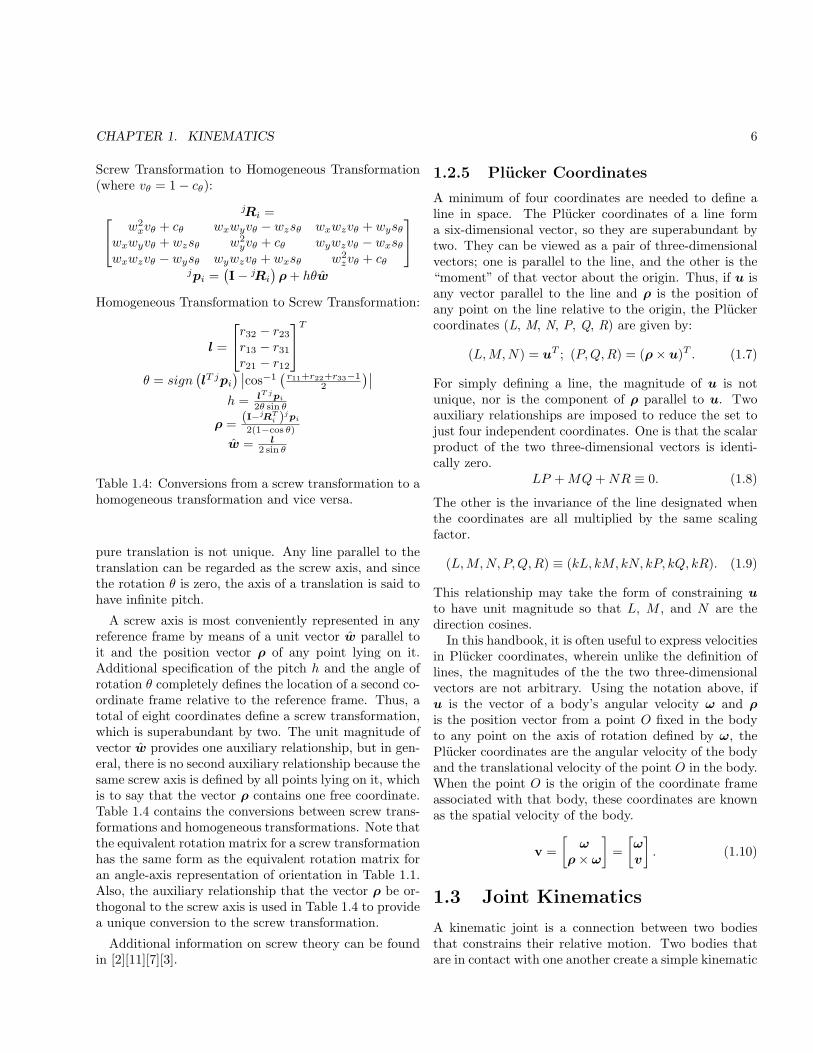
Screw Transformation to Homogeneous Transformation(where v% = 1" c%):

jRi =#

$w2

xv% + c% wxwyv% " wzs% wxwzv% + wys%

wxwyv% + wzs% w2yv% + c% wywzv% " wxs%

wxwzv% " wys% wywzv% + wxs% w2zv% + c%

%

&

jpi =*I" jRi

+! + h%w

Homogeneous Transformation to Screw Transformation:

l =

#

$r32 " r23

r13 " r31

r21 " r12

%

&T

% = sign*lT jpi

+ ..cos!1*

r11+r22+r33!12

+..

h = lT jpi

2% sin %

! = (I!jRTi )jpi

2(1!cos %)

w = l2 sin %

Table 1.4: Conversions from a screw transformation to ahomogeneous transformation and vice versa.

pure translation is not unique. Any line parallel to thetranslation can be regarded as the screw axis, and sincethe rotation % is zero, the axis of a translation is said tohave infinite pitch.

A screw axis is most conveniently represented in anyreference frame by means of a unit vector w parallel toit and the position vector ! of any point lying on it.Additional specification of the pitch h and the angle ofrotation % completely defines the location of a second co-ordinate frame relative to the reference frame. Thus, atotal of eight coordinates define a screw transformation,which is superabundant by two. The unit magnitude ofvector w provides one auxiliary relationship, but in gen-eral, there is no second auxiliary relationship because thesame screw axis is defined by all points lying on it, whichis to say that the vector ! contains one free coordinate.Table 1.4 contains the conversions between screw trans-formations and homogeneous transformations. Note thatthe equivalent rotation matrix for a screw transformationhas the same form as the equivalent rotation matrix foran angle-axis representation of orientation in Table 1.1.Also, the auxiliary relationship that the vector ! be or-thogonal to the screw axis is used in Table 1.4 to providea unique conversion to the screw transformation.

Additional information on screw theory can be foundin [2][11][7][3].

1.2.5 Plucker Coordinates

A minimum of four coordinates are needed to define aline in space. The Plucker coordinates of a line forma six-dimensional vector, so they are superabundant bytwo. They can be viewed as a pair of three-dimensionalvectors; one is parallel to the line, and the other is the“moment” of that vector about the origin. Thus, if u isany vector parallel to the line and ! is the position ofany point on the line relative to the origin, the Pluckercoordinates (L, M, N, P, Q, R) are given by:

(L,M,N) = uT ; (P,Q,R) = (!! u)T . (1.7)

For simply defining a line, the magnitude of u is notunique, nor is the component of ! parallel to u. Twoauxiliary relationships are imposed to reduce the set tojust four independent coordinates. One is that the scalarproduct of the two three-dimensional vectors is identi-cally zero.

LP + MQ + NR $ 0. (1.8)

The other is the invariance of the line designated whenthe coordinates are all multiplied by the same scalingfactor.

(L,M,N,P, Q,R) $ (kL, kM, kN, kP, kQ, kR). (1.9)

This relationship may take the form of constraining uto have unit magnitude so that L, M , and N are thedirection cosines.

In this handbook, it is often useful to express velocitiesin Plucker coordinates, wherein unlike the definition oflines, the magnitudes of the the two three-dimensionalvectors are not arbitrary. Using the notation above, ifu is the vector of a body’s angular velocity " and !is the position vector from a point O fixed in the bodyto any point on the axis of rotation defined by ", thePlucker coordinates are the angular velocity of the bodyand the translational velocity of the point O in the body.When the point O is the origin of the coordinate frameassociated with that body, these coordinates are knownas the spatial velocity of the body.

v =,

"!! "

-=

,"v

-. (1.10)

1.3 Joint Kinematics

A kinematic joint is a connection between two bodiesthat constrains their relative motion. Two bodies thatare in contact with one another create a simple kinematic

CHAPTER 1. KINEMATICS 7

joint. The surfaces of the two bodies that are in con-tact are able to move over one another, thereby permit-ting relative motion of the two bodies. Simple kinematicjoints are classified as lower pair joints if contact occursover surfaces and as higher pair joints if contact occursonly at points or along lines. Lower pair joints are me-chanically attractive since wear is spread over the wholesurface and lubricant is trapped in the small clearancespace (in non-idealized systems) between the surfaces, re-sulting in relatively good lubrication. As can be provedfrom the requirement for surface contact [Ref], there areonly six possible forms of lower pair: revolute, prismatic,helical, cylindrical, spherical, and planar joints.

Some higher pair joints also have attractive properties,particularly rolling pairs in which one body rolls withoutslipping over the surface of the other. This is mechan-ically attractive since the absence of sliding means theabsence of abrasive wear. However, since contact occursat a point, or along a line, application of a load acrossthe joint may lead to very high local stresses resulting inother forms of material failure and, hence, wear. Higherpair joints can be used to create kinematic joints withspecial geometric properties, as in the case of a gear pair,or a cam and follower pair.

Compound kinematic joints are connections betweentwo bodies formed by chains of other members and sim-ple kinematic joints. A compound joint may constrainthe relative motion of the two bodies joined in the sameway as a simple joint. In such a case, the two joints aresaid to be kinematically equivalent. An example is a ballbearing that provides the same constraint as a revolutejoint but is composed of a set of bearing balls trappedbetween two journals. The balls ideally roll without slip-ping on the journals, thereby taking advantage of thespecial properties of rolling contact joints.

Additional information on joints can be found in Chap-ter 4 Mechanisms and Actuation.

1.3.1 Revolute

The most general form of a revolute joint, sometimes re-ferred to colloquially as a hinge or pin joint, is a lowerpair composed of two congruent surfaces of revolution.The surfaces are the same except one of them is an ex-ternal surface, convex in any plane normal to the axis ofrevolution, and one is an internal surface, concave in anyplane normal to the axis. The surfaces may not be solelyin the form of right circular cylinders, since surfaces ofthat form do not provide any constraint on axial slid-ing. A revolute joint permits only rotation of one of the

bodies joined relative to the other. The position of onebody relative to the other may be expressed as the anglebetween two lines normal to the joint axis, one fixed ineach body. Thus, the joint has one degree of freedom.As noted above, a revolute joint is often realized as acompound joint. Revolute joints are easily actuated byrotating motors and are, therefore, extremely commonin robotic systems. They may also be present as passive,unactuated joints.

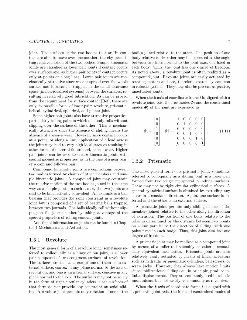
When the z axis of coordinate frame i is aligned with arevolute joint axis, the free modes #i and the constrainedmodes #c

i of the joint are expressed as,

#i =

#

//////$

001000

%

000000&, #c

i =

#

//////$

1 0 0 0 00 1 0 0 00 0 0 0 00 0 1 0 00 0 0 1 00 0 0 0 1

%

000000&. (1.11)

1.3.2 Prismatic

The most general form of a prismatic joint, sometimesreferred to colloquially as a sliding joint, is a lower pairformed from two congruent general cylindrical surfaces.These may not be right circular cylindrical surfaces. Ageneral cylindrical surface is obtained by extruding anycurve in a constant direction. Again, one surface is in-ternal and the other is an external surface.

A prismatic joint permits only sliding of one of themembers joined relative to the other along the directionof extrusion. The position of one body relative to theother is determined by the distance between two pointson a line parallel to the direction of sliding, with onepoint fixed in each body. Thus, this joint also has onedegree of freedom.

A prismatic joint may be realized as a compound jointby means of a roller-rail assembly or other kinemati-cally equivalent mechanism. Prismatic joints are alsorelatively easily actuated by means of linear actuatorssuch as hydraulic or pneumatic cylinders, ball screws, orscrew jacks. However, they always have motion limitssince unidirectional sliding can, in principle, produce in-finite displacements. They are commonly used in roboticmechanisms, but not nearly as commonly as revolutes.

When the z axis of coordinate frame i is aligned witha prismatic joint axis, the free and constrained modes of

CHAPTER 1. KINEMATICS 8

the joint are expressed as,

#i =

#

//////$

000001

%

000000&, #c

i =

#

//////$

1 0 0 0 00 1 0 0 00 0 1 0 00 0 0 1 00 0 0 0 10 0 0 0 0

%

000000&. (1.12)

1.3.3 Helical

The most general form of a helical joint, sometimes re-ferred to colloquially as a screw joint, is a lower pairformed from two helicoidal surfaces formed by extrudingany curve along a helical path. The simple example isa screw and nut wherein the basic generating curve isa pair of straight lines. The angle of rotation about theaxis of the screw joint % is directly related to the distanceof displacement of one body relative to the other alongthat axis d by the expression d = h%, where the constanth is called the pitch of the screw. Screw joints are mostoften found in robotic mechanisms as constituents of lin-ear actuators such as screw jacks and ball screws. Theyare seldom used as primary kinematic joints.

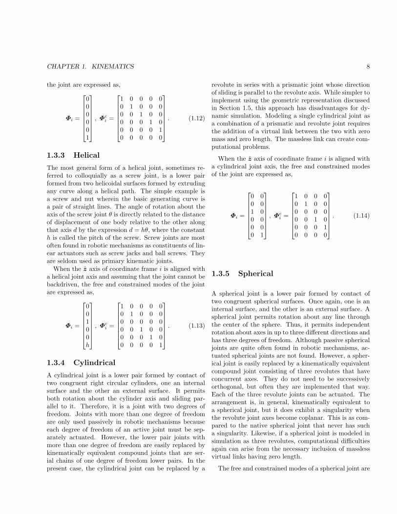
When the z axis of coordinate frame i is aligned witha helical joint axis and assuming that the joint cannot bebackdriven, the free and constrained modes of the jointare expressed as,

#i =

#

//////$

00100h

%

000000&, #c

i =

#

//////$

1 0 0 0 00 1 0 0 00 0 0 0 00 0 1 0 00 0 0 1 00 0 0 0 1

%

000000&. (1.13)

1.3.4 Cylindrical

A cylindrical joint is a lower pair formed by contact oftwo congruent right circular cylinders, one an internalsurface and the other an external surface. It permitsboth rotation about the cylinder axis and sliding par-allel to it. Therefore, it is a joint with two degrees offreedom. Joints with more than one degree of freedomare only used passively in robotic mechanisms becauseeach degree of freedom of an active joint must be sep-arately actuated. However, the lower pair joints withmore than one degree of freedom are easily replaced bykinematically equivalent compound joints that are ser-ial chains of one degree of freedom lower pairs. In thepresent case, the cylindrical joint can be replaced by a

revolute in series with a prismatic joint whose directionof sliding is parallel to the revolute axis. While simpler toimplement using the geometric representation discussedin Section 1.5, this approach has disadvantages for dy-namic simulation. Modeling a single cylindrical joint asa combination of a prismatic and revolute joint requiresthe addition of a virtual link between the two with zeromass and zero length. The massless link can create com-putational problems.

When the z axis of coordinate frame i is aligned witha cylindrical joint axis, the free and constrained modesof the joint are expressed as,

#i =

#

//////$

0 00 01 00 00 00 1

%

000000&, #c

i =

#

//////$

1 0 0 00 1 0 00 0 0 00 0 1 00 0 0 10 0 0 0

%

000000&. (1.14)

1.3.5 Spherical

A spherical joint is a lower pair formed by contact oftwo congruent spherical surfaces. Once again, one is aninternal surface, and the other is an external surface. Aspherical joint permits rotation about any line throughthe center of the sphere. Thus, it permits independentrotation about axes in up to three di!erent directions andhas three degrees of freedom. Although passive sphericaljoints are quite often found in robotic mechanisms, ac-tuated spherical joints are not found. However, a spher-ical joint is easily replaced by a kinematically equivalentcompound joint consisting of three revolutes that haveconcurrent axes. They do not need to be successivelyorthogonal, but often they are implemented that way.Each of the three revolute joints can be actuated. Thearrangement is, in general, kinematically equivalent toa spherical joint, but it does exhibit a singularity whenthe revolute joint axes become coplanar. This is as com-pared to the native spherical joint that never has sucha singularity. Likewise, if a spherical joint is modeled insimulation as three revolutes, computational di"cultiesagain can arise from the necessary inclusion of masslessvirtual links having zero length.

The free and constrained modes of a spherical joint are

CHAPTER 1. KINEMATICS 9

expressed as,

#i =

#

//////$

1 0 00 1 00 0 10 0 00 0 00 0 0

%

000000&, #c

i =

#

//////$

0 0 00 0 00 0 01 0 00 1 00 0 1

%

000000&. (1.15)

1.3.6 Planar

A planar joint is formed by planar contacting surfaces.Like the spherical joint, it is a lower pair joint with threedegrees of freedom. Passive planar joints are occasionallyfound in robotic mechanisms. A kinematically equiva-lent compound joint consisting of a serial chain of threerevolutes with parallel axes can replace a planar joint.As was the case with the spherical joint, the compoundjoint exhibits a singularity when the revolute axes be-come coplanar.

When the z axis of coordinate frame i is aligned withthe normal to the plane of contact, the free and con-strained modes of the joint are expressed as,

#i =

#

//////$

0 0 00 0 01 0 00 1 00 0 10 0 0

%

000000&, #c

i =

#

//////$

1 0 00 1 00 0 00 0 00 0 00 0 1

%

000000&. (1.16)

1.3.7 Universal

A universal joint, often referred to as a Cardan or Hookejoint, is a compound joint with two degrees of freedom.It consists of a serial chain of two revolutes whose axesintersect orthogonally and is used in robotic mechanismsin both active and passive forms.

1.3.8 Rolling Contact

Rolling contact actually encompasses several di!erentgeometries. Planar rolling contact requires that themechanism in which the joint is used constrain the rela-tive motion to a plane. This is the case of a roller bearing,for example. Rolling contact in planar motion permitsone degree of freedom of relative motion. As was notedabove, rolling contact has desirable wear properties sincethe absence of sliding means the absence of abrasivewear. Planar rolling contact can take place along a line,thereby spreading the load and wear somewhat. Three-dimensional rolling contact allows rotation about any

axis through the point of contact that is, in principle,unique. Hence, a three-dimensional rolling contact pairpermits relative motion with three degrees of freedom.

1.3.9 Holonomic and Non-HolonomicConstraints

With the exception of rolling contact, all of the con-straints associated with the joints discussed in the pre-ceding sections can be expressed mathematically byequations containing only the joint position variables.These are called holonomic constraints. The number ofequations, and hence the number of constraints, is 6"n,where n is the number of degrees of freedom of the joint.The constraints are intrinsically part of the axial jointmodel.

A non-holonomic constraint is one that cannot be ex-pressed in terms of the position variables alone, but in-cludes the time derivative of one or more of those vari-ables. These constraint equations cannot be integratedto obtain relationships solely between the joint variables.The most common example in robotic systems arisesfrom the use of a wheel or roller that rolls without slip-ping on another member.

1.3.10 Generalized Coordinates

In a robot manipulator consisting of N bodies, 6N co-ordinates are required to specify the position and orien-tation of all the bodies relative to a coordinate frame.Since some of those bodies are jointed together, a num-ber of constraint equations will establish relationshipsbetween some of these coordinates. In this case, the 6Ncoordinates can be expressed as functions of a smallerset of coordinates q that are all independent. The coor-dinates in this set are known as generalized coordinates,and motions associated with these coordinates are con-sistent with all of the constraints. The joint variables qof a robot manipulator form a set of generalized coordi-nates.

1.4 Workspace

Most generally, the workspace of a robotic manipula-tor is the total volume swept out by the end-e!ectoras the manipulator executes all possible motions. Theworkspace is determined by the geometry of the manip-ulator and the limits of the joint motions. It is morespecific to define the reachable workspace as the totallocus of points at which the end-e!ector can be placed

CHAPTER 1. KINEMATICS 10

and the dextrous workspace as the subset of those pointsat which the end-e!ector can be placed while having anarbitrary orientation. Dexterous workspaces exist onlyfor certain idealized geometries, so real industrial ma-nipulators with joint motion limits almost never possessdexterous workspaces.

Many serial-chain robotic manipulators are designedsuch that their joints can be partitioned into a regionalstructure and an orientation structure. The joints inthe regional structure accomplish the positioning of theend-e!ector in space, and the joints in the orientationstructure accomplish the orientation of the end-e!ector.Typically, the inboard joints of a serial chain manipula-tor comprise the regional structure, while the outboardjoints comprise the orientation structure. Also, sinceprismatic joints provide no capability for rotation, theyare generally not employed within the orientation struc-ture.

The regional workspace volume can be calculated fromthe known geometry of the serial-chain manipulator andmotion limits of the joints. With three inboard jointscomprising the regional structure, the area of workspacefor the outer two (joints 2 and 3) is computed first, andthen the volume is calculated by integrating over thejoint variable of the remaining inboard joint (joint 1). Inthe case of a prismatic joint, this simply involves multi-plying the area by the total length of travel of the pris-matic joint. In the more common case of a revolute joint,it involves rotating the area about the joint axis throughthe full range of motion of the revolute. By the Theoremof Pappus, the associated volume is equal to the productof the area, the distance from the area’s centroid to theaxis, and the angle through which the area is rotated.The boundaries of the area are determined by tracingthe motion of a reference point in the end-e!ector, typ-ically the center of rotation of the wrist that serves asthe orientation structure. Starting with each of the twojoints at motion limits and with joint 2 locked, joint 3 ismoved until its second motion limit is reached. Joint 3is then locked, and joint 2 is freed to move to its secondmotion limit. Joint 2 is again locked, while joint 3 isfreed to move back to its original motion limit. Finally,joint 3 is locked, and joint 2 freed to move likewise toits original motion limit. In this way, the trace of thereference point is a closed curve whose area and centroidcan be calculated mathematically.

More details on manipulator workspace can be foundin Chapter 4 Mechanisms and Actuation and Chapter 11Design Criteria.

1.5 Geometric Representation

The geometry of a robotic manipulator is convenientlydefined by attaching coordinate frames to each link.While these frames could be located arbitrarily, it is ad-vantageous both for consistency and computational e"-ciency to adhere to a convention for locating the frameson the links. Denavit and Hartenberg [8] introduced thefoundational convention that has been adapted in a num-ber of di!erent ways, one of which is the convention intro-duced by Khalil and Dombre [12] used throughout thishandbook. In all of its forms, the convention requiresonly four rather than six parameters to locate one coor-dinate frame relative to another. The four parametersare the link length ai, the link twist !i, the joint o!setdi, and the joint angle %i. This parsimony is achievedthrough judicious placement of the coordinate frame ori-gins and axes such that the x axis of one frame bothintersects and is perpendicular to the z axis of the pre-ceding coordinate frame. The convention is applicable tomanipulators consisting of revolute and prismatic joints,so when multi-degree-of-freedom joints are present, theyare modeled as combinations of revolute and prismaticjoints, as discussed in Section 1.3.

There are essentially four di!erent forms of the con-vention for locating coordinate frames in a robotic mech-anism. Each exhibits its own advantages by managingtrade-o!s of intuitive presentation. In the original De-navit and Hartenberg [8] convention, joint i is locatedbetween links i and i + 1, so it is on the outboard sideof link i. Also, the joint o!set di and joint angle %i aremeasured along and about the i " 1 joint axis, so thesubscripts of the joint parameters do not match that ofthe joint axis. Waldron [35] and Paul [22] modified thelabeling of axes in the original convention such that jointi is located between links i" 1 and i in order to make itconsistent with the base member of a serial chain beingmember 0. This places joint i at the inboard side of linki and is the convention used in all of the other modi-fied versions. Furthermore, Waldron and Paul addressedthe mismatch between subscripts of the joint parametersand joint axes by placing the zi axis along the i+1 jointaxis. This, of course, relocates the subscript mismatchto the correspondence between the joint axis and the zaxis of the coordinate frame. Craig [6] eliminated all ofthe subscript mismatches by placing the zi axis alongjoint i, but at the expense of the homogeneous trans-form i!1T i being formed with a mixture of joint para-meters with subscript i and link parameters with sub-script i" 1. Khalil and Dombre [12] introduced another

CHAPTER 1. KINEMATICS 11

Geometric ParametersDiagram

Figure 1.1: place holder

variation similar to Craig’s except that it defines the linkparameters ai and !i along and about the xi!1 axis. Inthis case, the homogeneous transform i!1T i is formedonly with parameters with subscript i, and the subscriptmismatch is such that ai and !i indicate the length andtwist of link i" 1 rather than link i. Thus, in summary,the advantages of the convention used throughout thishandbook compared to the alternative conventions arethat the z axes of the coordinate frames share the com-mon subscript of the joint axes, and the four parametersthat define the spatial transform from coordinate frame ito coordinate frame i"1 all share the common subscripti.

In this handbook, the convention for serial chain ma-nipulators is shown in Figure 1.1 and summarized as fol-lows:

1. The N moving bodies of the robotic mechanism arenumbered from 1 to N . The number of the base is0.

2. The N joints of the robotic mechanism are num-bered from 1 to N , with joint i located betweenmembers i" 1 and i.

3. The zi axis is located along the axis of joint i.

4. The xi axis is located along the common normalbetween the zi!1 and zi axes.

5. ai is the distance from zi!1 to zi along xi!1.

6. !i is the angle from zi!1 to zi about xi!1.

7. di is the distance from xi!1 to xi along zi.

8. %i is the angle from xi!1 to xi about zi.

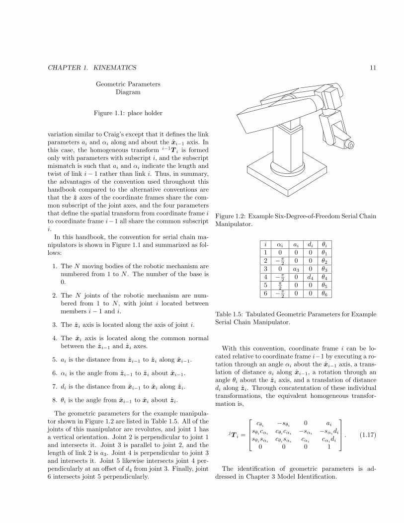
The geometric parameters for the example manipula-tor shown in Figure 1.2 are listed in Table 1.5. All of thejoints of this manipulator are revolutes, and joint 1 hasa vertical orientation. Joint 2 is perpendicular to joint 1and intersects it. Joint 3 is parallel to joint 2, and thelength of link 2 is a3. Joint 4 is perpendicular to joint 3and intersects it. Joint 5 likewise intersects joint 4 per-pendicularly at an o!set of d4 from joint 3. Finally, joint6 intersects joint 5 perpendicularly.

Figure 1.2: Example Six-Degree-of-Freedom Serial ChainManipulator.

i !i ai di %i

1 0 0 0 %1

2 "'2 0 0 %2

3 0 a3 0 %3

4 "'2 0 d4 %4

5 '2 0 0 %5

6 "'2 0 0 %6

Table 1.5: Tabulated Geometric Parameters for ExampleSerial Chain Manipulator.

With this convention, coordinate frame i can be lo-cated relative to coordinate frame i"1 by executing a ro-tation through an angle !i about the xi!1 axis, a trans-lation of distance ai along xi!1, a rotation through anangle %i about the zi axis, and a translation of distancedi along zi. Through concatentation of these individualtransformations, the equivalent homogeneous transfor-mation is,

jT i =

#

//$

c%i "s%i 0 ai

s%ic!i c%ic!i "s!i "s!idi

s%is!i c%is!i c!i c!idi

0 0 0 1

%

00& . (1.17)

The identification of geometric parameters is ad-dressed in Chapter 3 Model Identification.

CHAPTER 1. KINEMATICS 12

1.6 Forward Kinematics

The forward kinematics problem for a serial chain ma-nipulator is to find the position and orientation of theend-e!ector relative to the base given the positions ofall of the joints and the values of all of the geometriclink parameters. A more general expression of the prob-lem is to find the relative position and orientation of anytwo designated members given the geometric structureof the manipulator and the values of a number of jointpositions equal to the number of degrees of freedom ofthe mechanism. The forward kinematics problem is crit-ical for developing manipulator coordination algorithmsbecause joint positions are typically measured by sensorsmounted on the joints and it is necessary to calculate thepositions of the joint axes relative to the fixed referenceframe.

In practice, the forward kinematics problem is solvedby calculating the transformation between a coordinateframe fixed in the end-e!ector and another coordinateframe fixed in the base. This is straightforward for aserial chain since the transformation describing the po-sition of the end-e!ector relative to the base is obtainedby simply concatenating transformations between framesfixed in adjacent links of the chain. The convention forthe geometric representation of a manipulator presentedin Section 1.5 reduces this to finding an equivalent 4! 4homogeneous transformation matrix that relates the spa-tial displacement of the end-e!ector coordinate frame tothe base coordinate frame.

For the example serial chain manipulator shown in Fig-ure 1.2, the transformation is,

0T 6 = 0T 11T 2

2T 33T 4

4T 55T 6. (1.18)

Table 1.6 contains the elements of 0T 6 that are calcu-lated using Table 1.5 and Equation 1.17.

Once again, homogeneous transformations provide acompact notation, but are computationally ine"cient forsolving the forward kinematics problem. A reduction incomputation can be achieved by separating the positionand orientation portions of the transformation to elimi-nate all multiplications by the 0 and 1 elements of thematrices.

The forward kinematics problem for closed chains ismuch more complicated because of the additional con-straints present. Solution methods for closed chains areincluded in Chapter 13 Kinematic Structure and Analy-sis.

0T 6 =

#

//$

r11 r12 r130px

6

r21 r22 r230py

6

r31 r32 r330pz

6

0 0 0 1

%

00&

r11 = c1 (s2s3 " c2c3) (s4s6 " c4c5c6)"c1s5c6 (c2s3 + s2c3) + s1 (s4c5c6 + c4s6) .

r21 = s1 (s2s3 " c2c3) (s4s6 " c4c5c6)"s1s5c6 (c2s3 + s2c3)" c1 (s4c5c6 + c4s6) .

r31 = (c2s3 + s2c3) (s4s6 " c4c5c6)+s5c6 (s2s3 " c2c3) .

r12 = c1 (s2s3 " c2c3) (c4c5s6 + s4c6)+c1s5s6 (c2s3 + s2c3) + s1 (c4c6 " s4c5s6) .

r22 = s1 (s2s3 " c2c3) (c4c5s6 + s4c6)+s1s5s6 (c2s3 + s2c3)" c1 (c4c6 " s4c5s6) .

r32 = (c2s3 + s2c3) (c4c5s6 + s4c6)"s5s6 (s2s3 " c2c3) .

r13 = c1c4s5 (s2s3 " c2c3)" c1c5 (c2s3 + s2c3)"s1s4s5.

r23 = s1c4s5 (s2s3 " c2c3)" s1c5 (c2s3 + s2c3)+c1s4s5.

r33 = c4s5 (c2s3 + s2c3) + c5 (s2s3 " c2c3) .0px

6 = a2c1c2 " d4c1 (c2s3 + s2c3)0py

6 = a2s1c2 " d4s1 (c2s3 + s2c3)0pz

6 = "a2s2 + d4 (s2s3 " c2c3)

Table 1.6: Forward Kinematics of the Example SerialChain Manipulator in Figure 1.2.

1.7 Inverse Kinematics

The inverse kinematics problem for a serial chain ma-nipulator is to find the values of the joint positions giventhe position and orientation of the end-e!ector relativeto the base and the values of all of the geometric link pa-rameters. Once again, this is a simplified statement ap-plying only to serial chains. A more general statement is:Given the relative positions and orientations of two mem-bers of a mechanism, find the values of all of the jointpositions. This amounts to finding all of the joint posi-tions given the homogeneous transformation between thetwo members of interest. In the common case of a six-degree-of-freedom serial chain manipulator, the knowntransformation is 0T 6. Reviewing the formulation ofthis transformation in Section 1.6, it is clear that theinverse kinematics problem for serial chain manipulatorsrequires the solution of non-linear sets of equations. Inthe case of a six-degree-of-freedom manipulator, three ofthese equations relate to the position vector within thehomogeneous transform, and the other three relate to therotation matrix. In the latter case, these three equations

CHAPTER 1. KINEMATICS 13

cannot come from the same row or column because ofthe dependency within the rotation matrix. With thesenon-linear equations, it is possible that no solutions ex-ist or multiple solutions exist. For a solution to exist,the desired position and orientation of the end-e!ectormust lie in the workspace of the manipulator. In caseswhere solutions do exist, they often cannot be presentedin closed form, so numerical methods are required.

1.7.1 Closed-Form Solutions

Closed-form solutions are desirable because they arefaster than numerical solutions and readily identify allpossible solutions. The disadvantage of closed-form solu-tions are that they are not general, but robot-dependent.The most e!ective methods for finding closed-form solu-tions are ad hoc techniques that take advantage of partic-ular geometric features of specific mechanisms. In gen-eral, closed-form solutions can only be obtained for six-degree-of-freedom systems with special kinematic struc-ture characterized by a large number of the geometric pa-rameters defined in Section 1.5 being zero-valued. Mostindustrial manipulators have such structure because itpermits more e"cient coordination software. Su"cientconditions for a six-degree-of-freedom manipulator tohave closed-form inverse kinematics solutions are [26]: 1)three consecutive revolute joint axes intersect at a com-mon point, as in a spherical wrist; 2) three consecutiverevolute joint axes are parallel.

Closed-form solution approaches are generally dividedinto algebraic and geometric methods.

Algebraic Methods

Algebraic methods involve identifying the significantequations containing the joint variables and manipulat-ing them into a soluble form. A common strategy is re-duction to a transcendental equation in a single variablesuch as,

C1 cos %i + C2 sin %i + C3 = 0, (1.19)

where C1, C2, and C3 are constants. The solution tosuch an equation is,

%i = 2 tan!1

1C2 ±

(C2

2 " C23 + C2

1

C1 " C3

2. (1.20)

Special cases in which one or more of the constants arezero are also common. Reduction to a pair of equationshaving the form,

C1 cos %i + C2 sin %i + C3 = 0

%1 =%3 =%2 =

Table 1.7: Inverse Position Kinematics of the ArticulatedArm Within the Example Serial Chain Manipulator inFigure 1.2.

%4 =%5 =%6 =

Table 1.8: Inverse Orientation Kinematics of the Spheri-cal Wrist Within the Example Serial Chain Manipulatorin Figure 1.2.

C1 sin %i " C2 cos %i + C4 = 0, (1.21)

is particularly useful because only one solution results,

%i = Atan2 ("C1C4 " C2C3, C2C4 " C1C3) . (1.22)

Geometric Methods

Geometric methods involve identifying points on the ma-nipulator relative to which position and/or orientationcan be expressed as a function of a reduced set of thejoint variables. This often amounts to decomposing thespatial problem into separate planar problems. The re-sulting equations are solved using algebraic manipula-tion. The two su"cient conditions for existence of aclosed-form solution for a six-degree-of-freedom manip-ulator that are listed above enable the decomposition ofthe problem into inverse position kinematics and inverseorientation kinematics. This is the decomposition intoregional and orientation structures discussed in Section1.4, and the solution is found by rewriting Equation 1.18,

(1.23)

The example manipulator in Figure 1.2 has this struc-ture, and regional structure is commonly known as anarticulated or anthropomorphic arm or an elbow manip-ulator. The solution to the inverse position kinemat-ics problem for such a structure is summarized in Ta-ble 1.7.1. The orientation structure is simply a spheri-cal wrist, and the corresponding solution to the inverseorientation kinematics problem is summarized in Table1.7.1.

CHAPTER 1. KINEMATICS 14

1.7.2 Numerical Methods

Unlike the algebraic and geometric methods used tofind closed-form solutions, numerical methods are notrobot-dependent, so they can be applied to any kine-matic structure. The disadvantages of numerical meth-ods are that they can be slower and in some cases, theydo not allow computation of all possible solutions. For asix-degree-of-freedom serial chain manipulator with onlyrevolute and prismatic joints, the translation and rota-tion equations can always be reduced to a polynomial ina single variable of degree not greater than 16 [15]. Thus,such a manipulator can have as many as sixteen real solu-tions to the inverse kinematics problem [18]. Since closedform solution of a polynomial equation is only possibleif the polynomial is of degree four or less, it follows thatmany manipulator geometries are not soluble in closedform. In general, a greater number of non-zero geometricparameters corresponds to a polynomial of higher degreein the reduction. For such manipulator structures, themost common numerical methods can be divided intocategories of symbolic elimination methods, continuationmethods, and interative methods.

Symbolic Elimination Methods

Symbolic elimination methods involve analytical manip-ulations to eliminate variables from the system of non-linear equations to reduce it to a smaller set of equa-tions. Raghavan and Roth [27] used dialytic eliminationto reduce the inverse kinematics problem of a generalsix-revolute serial chain manipulator to a polynomial ofdegree 16 and to find all possible solutions. The rootsprovide solutions for one of the joint variables, while theother variables are computed by solving linear systems.Manocha and Canny [17] improved the numerical prop-erties of this technique by reformulating the problem as ageneralized eigenvalue problem. An alternative approachto elimination makes use of Grobner bases [4][13].

Continuation Methods

Continuation methods involve tracking a solution pathfrom a start system with known solutions to a targetsystem whose solutions are sought as the start systemis transformed into the target system. These techniqueshave been applied to inverse kinematics problems [33],and special properties of polynomial systems can be ex-ploited to find all possible solutions [36].

Iterative Methods

A number of di!erent iterative methods can be employedto solve the inverse kinematics problem. Most of themconverge to a single solution based on an initial guess,so the quality of that guess greatly impacts the solutiontime. Newton-Raphson methods provide a fundamen-tal approach that uses a first-order approximation to theoriginal equations. Pieper [26] was among the first toapply the method to inverse kinematics, and others havefollowed [32][19]. Optimization approaches formulate theproblem as a nonlinear optimization problem and employsearch techniques to move from an initial guess to a so-lution [34][40]. Resolved motion rate control convertsthe problem to a di!erential equation [37], and a mod-ified predictor-corrector algorithm can be used to per-form the joint velocity integration [5]. Control-theory-based methods cast the di!erential equation into a con-trol problem [29]. Interval analysis [28] is perhaps oneof the most promising iterative methods because it o!ersrapid convergence to a solution and can be used to findall possible solutions.

1.8 Forward Instantaneous Kine-matics

The forward instantaneous kinematics problem for a ser-ial chain manipulator is: Given the positions of all mem-bers of the chain and the rates of motion about all thejoints, find the total velocity of the end-e!ector. Herethe rate of motion about the joint is the angular ve-locity of rotation about a revolute joint or the transla-tional velocity of sliding along a prismatic joint. Thetotal velocity of a member is the velocity of the originof the reference frame fixed to it combined with its an-gular velocity. That is, the total velocity has six in-dependent components and therefore, completely repre-sents the velocity field of the member. It is important tonotice that this definition includes an assumption thatthe position of the mechanism is completely known. Inmost situations, this means that either the forward orinverse position kinematics problem must be solved be-fore the forward instantaneous kinematics problem canbe addressed. The same is true of the inverse instanta-neous kinematics problem discussed in the following sec-tion. The forward instantaneous kinematics problem isimportant when doing acceleration analysis for the pur-pose of studying dynamics. The total velocities of themembers are needed for the computation of Coriolis and

CHAPTER 1. KINEMATICS 15

centripetal acceleration components.Di!erentiation with respect to time of the forward po-

sition kinematics equations yields a set of equations ofthe form,

vN = J(q)q (1.24)

where vN is the spatial velocity of the end-e!ector, qis an N -dimensional vector composed of the joint rates,and J(q) is a 6!N matrix whose elements are, in gen-eral, non-linear functions of q1, ..., qN . J(q) is calledthe Jacobian matrix of this algebraic system. If the jointpositions are known, Equation 1.24 yields six linear al-gebraic equations in the joint rates. If the joint ratesare given, solution of Equation 1.24 is a solution of theforward instantaneous kinematics problem. Notice thatJ(q) can be regarded as a known matrix for this purposeprovided all the joint positions are known.

1.8.1 Jacobian

Formulation of the Jacobian. Di!erentiation of posi-tion equations. From screw parameters. Development ofequation for transforming the Jacobian from one frameto another.

Table 1.8.1 contains the Jacobian of the example ma-nipulator show in Figure 1.2.

Additional information about Jacobians can be foundin Chapter 12 Kinematically Redundant Manipulators.

1.9 Inverse Instantaneous Kine-matics

The important problem from the point of view of ro-botic coordination is the inverse instantaneous kinemat-ics problem. The inverse instantaneous kinematics prob-lem for a serial chain manipulator is: Given the positionsof all members of the chain and the total velocity of theend-e!ector, find the rates of motion of all joints. Whencontrolling a movement of an industrial robot which op-erates in the point-to-point mode, it is not only necessaryto compute the final joint positions needed to assume thedesired final hand position. It is also necessary to gen-erate a smooth trajectory for motion between the ini-tial and final positions. There are, of course, an infinitenumber of possible trajectories for this purpose. How-ever, the most straightforward and successful approachemploys algorithms based on the solution of the inverseinstantaneous kinematics problem. This technique orig-inated in the work of Whitney [38] and of Pieper [26].

J =

#

//$

J11 J12 J13 J14

J21 J22 J23 J24

J31 J32 J33 J34

J41 J42 J43 J44

%

00&

J11 =J21 =J31 =J41 =J12 =J22 =J32 =J42 =J13 =J23 =J33 =J43 =J14 =J24 =J34 =J44 =

Table 1.9: Forward Kinematics of the Example SerialChain Manipulator in Figure 1.2.

1.9.1 Inverse Jacobian

In order to solve the linear system of equations in thejoint rates obtained by decomposing Equation 1.24 intoits component equations when v is known, it is necessaryto invert the Jacobian matrix. The equation becomes,

q = J!1(q)vN (1.25)

Since J is a 6 ! 6 matrix, numerical inversion is notvery attractive in real-time software which must run atcomputation cycle rates of the order of 100 Hz or more.Worse, it is quite possible for J to become singular(|J | = 0). The inverse does not then exist. Even whenthe Jacobian matrix does not become singular, it maybecome ill conditioned leading to degraded performancein significant portions of the manipulator’s workspace.Most industrial robot geometries are simple enough thatthe Jacobian matrix can be inverted analytically leadingto a set of explicit equations for the joint rates. Thisgreatly reduces the number of computation operationsneeded as compared to numerical inversion.

More information on singularities can be found inChapter 4 Mechanisms and Actuation and Chapter 13Kinematic Structure and Analysis.

CHAPTER 1. KINEMATICS 16

1.10 Static Wrench Transmission

Static wrench analysis of a manipulator establishes therelationship between wrenches applied to the end-e!ectorand forces/torques applied to the joints. Through thepriniciple of virtual work, this relationship can be shownto be,

$ = JT f . (1.26)

1.11 Conclusions and FurtherReading

A number of excellent texts provide a broad introduc-tion to robotics with significant focus on kinematics[1][6][12][16][22][29][30][31][39][20].

Bibliography

[1] H. Asada and J.-J. E. Slotine, Robot Analysis and Con-trol, New York: John Wiley & Sons, 1986.

[2] R. S. Ball, A Treatise on the Theory of Screws, Cam-bridge: Cambridge University Press, 1998.

[3] O. Bottema and B. Roth, Theoretical Kinematics, NewYork: Dover Publications, 1990.

[4] B. Buchberger, “Applications of Grobner Basis in Non-Linear Computational Geometry,” Trends in ComputerAlgebra. Lecture Notes in Computer Science, vol. 296,Springer Verlag, 1989.

[5] H. Cheng and K. Gupta, “A Study of Robot InverseKinematics Based Upon the Solution of Di!erentialEquations,” Journal of Robotic Systems, vol. 8, no. 2,pp. 115–175, 1991.

[6] J. J. Craig, Introduction to Robotics: Mechanics andControl, Reading, MA: Addison-Wesley, 1986.

[7] J. K. Davidson and K. H. Hunt, Robots and Screw The-ory: Applications of Kinematics and Statics to Robotics,Oxford: Oxford University Press, 2004.

[8] J. Denavit and R. S. Hartenberg, “A Kinematic No-tation for Lower-Pair Mechanisms Based on Matrices,”Journal of Applied Mechanics, vol. 22, pp. 215–221,1955.

[9] J. Du!y, Analysis of Mechanisms and Robot Manipula-tors, New York: Wiley, 1980.

[10] K. S. Fu, R. C. Gonzalez, and C. S. G. Lee, Robotics:Control, Sensing, Vision, and Intelligence, New York:McGraw-Hill, 1987.

[11] K. H. Hunt, Kinematic Geometry of Mechanisms, Ox-ford: Clarendon Press, 1978.

[12] W. Khalil and E. Dombre, Modeling, Identification andControl of Robots, New York: Taylor & Francis, 2002.

[13] P. Kovacs, “Minimum Degree Solutions for the InverseKinematics Problem by Application of the BuchbergerAlgorithm,” Advances in Robot Kinematics, S. Stifterand J. Lenarcic Eds., Springer Verlag, pp. 326–334,1991.

[14] C. S. G Lee, “Robot Arm Kinematics, Dynamics, andControl,” Computer, vol. 15, no. 12, pp. 62-80, 1982.

[15] H. Y. Lee and C. G. Liang, “A New Vector Theory forthe Analysis of Spatial Mechanisms,” Mechanisms andMachine Theory, vol. 23, no. 3, pp. 209–217, 1988.

[16] F. L. Lewis, C. T. Abdallah, and D. M. Dawson, Controlof Robot Manipulators, New York: Macmillan, 1993.

[17] D. Manocha and J. Canny, Real Time Inverse Kine-matics for General 6R Manipulators, Technical report,University of California, Berkeley, 1992.

[18] R. Manseur and K. L. Doty, “A Robot Manipulatorwith 16 Real Inverse Kinematic Solutions,” Interna-tional Journal of Robotics Research, vol. 8, no. 5, pp.75–79, 1989.

[19] R. Manseur and K. L. Doty, “Fast Inverse Kinematicsof 5-Revolute-Axis Robot Maniputlators,” Mechanismsand Machine Theory, vol. 27, no. 5, pp. 587–597, 1992.

[20] R. M. Murray, Z. Li, and S. S. Sastry, A MathematicalIntroduction to Robotic Manipulation, Boca Raton, FL:CRC Press, 1994.

[21] D.E. Orin and W.W. Schrader, “E"cient Computationof the Jacobian for Robot Manipulators,” InternationalJournal of Robotics Research, vol. 3, no. 4, pp. 66–75,1984.

[22] R. Paul, Robot Manipulators: Mathematics, Program-ming and Control, Cambridge, MA: MIT Press, 1982.

[23] R. P. Paul, B. E. Shimano, and G. Mayer, “KinematicControl Equations for Simple Manipulators,” IEEETransactions on Systems, Man, and Cybernetics, vol.SMC-11, no. 6, pp. 339-455, 1981.

[24] R. P. Paul and C. N. Stephenson, “Kinematics of RobotWrists,” International Journal of Robotics Research, vol.20, no. 1, pp. 31–38, 1983.

[25] R. P. Paul and H. Zhang, “Computationally E"cientKinematics for Manipulators with Spherical wrists basedon the Homogeneous Transformation Representation,”International Journal of Robotics Research, vol. 5, no.2, pp. 32–44, 1986.

17

BIBLIOGRAPHY 18

[26] D. Pieper, The Kinematics of Manipulators Under Com-puter Control, Doctoral Dissertation, Stanford Univer-sity, 1968.

[27] M. Raghavan and B. Roth, “Kinematic Analysis of the6R Manipulator of General Geometry,” In Proceedings ofthe 5th International Symposium on Robotics Research,1990.

[28] R. S. Rao, A. Asaithambi, and S. K. Agrawal, “InverseKinematic Solution of Robot Manipulators Using Inter-val Analysis,” ASME Journal of Mechanical Design, vol.120, no. 1, pp. 147–150, 1998.

[29] L. Sciavicco and B. Siciliano, Modeling and Control ofRobot Manipulators, London: Springer, 2000.

[30] R. J. Schilling, Fundamentals of Robotics: Analysis andControl, Englewood Cli!s, NJ: Prentice-Hall, 1990.

[31] M. W. Spong and M. Vidyasagar, Robot Dynamics andControl, New York: John Wiley & Sons, 1989.

[32] S. C. A. Thomopoulos, and R. Y. J. Tam, “An IterativeSolution to the Inverse Kinematics of Robotic Manipu-lators,” Mechanisms and Machine Theory, vol. 26, no.4, pp. 359–373, 1991.

[33] L. W. Tsai and A. P. Morgan “Solving the Kinematicsof the Most General Six- and Five-Degree-of-FreedomManipulators by Continuation Methods,” ASME Jour-nal of Mechanisms, Transmissions, and Automation inDesign, vol. 107, pp. 189-195, 1985.

[34] J. J. Uicker, Jr., J. Denavit, and R. S. Hartenberg,“An Interactive Method for the Displacement Analysisof Spatial Mechanisms,” Journal of Applied Mechanics,vol. 31, pp. 309–314, 1964.

[35] K. J. Waldron, “A Study of Overconstrained LinkageGeometry by Solution of Closure Equations, Part I: AMethod of Study,” Mechanism and Machine Theory,vol. 8, no. 1, pp. 95–104, 1973.

[36] C. W. Wampler, A. P. Morgan, and A. J. Sommese,“Numerical Continuation Methods for Solving Polyno-mial Systems Arising in Kinematics,” ASME Journal ofMechanical Design, vol. 112, pp. 59-68, 1990.

[37] D. E. Whitney, “Resolved Motion Rate Control of Ma-nipulators and Human Prostheses,” IEEE Transactionson Man-Machine Systems, vol. 10, pp. 47–63, 1969.

[38] D. E. Whitney, ”The Mathematics of Coordinated Con-trol of Prosthetic Arms and Manipulators,” Journal ofDynamic Systems, Measurement, and Control, vol. 122,pp. 303–309, 1972.

[39] T. Yoshikawa, Foundations of Robotics, Cambridge,MA: MIT Press, 1990.

[40] J. Zhao and N. Badler, “Inverse Kinematics PositioningUsing Nonlinear Programming for Highly ArticulatedFigures,” Transactions on Computer Graphics, vol. 13,no. 4, pp. 313–336, 1994.