HABITAT ANALYSIS FOR THE SANTA YNEZ RIVER

Prepared for:

SANTA YNEZ RIVER CONSENSUS COMMITTEESanta Barbara, California

Prepared by:

SANTA YNEZ RIVER TECHNICAL ADVISORY COMMITTEESanta Barbara, California

March 1999

Cachuma Member Units Exhibit No. 226(b)

HABITAT ANALYSISFOR THE SANTA YNEZ RIVER

Prepared for:

SANTA YNEZ RIVER CONSENSUS COMMITTEESanta Barbara, California

Prepared by:

SANTA YNEZ RIVER TECHNICAL ADVISORY COMMITTEESanta Barbara, California

March 1999

Cachuma Member Units Exhibit No. 226(b)

i

TABLE OF CONTENTS

Page

1.0 Introduction.......................................................................................................... 1-1

2.0 Methods ............................................................................................................... 2-1

3.0 Results.................................................................................................................. 3-1

3.1 Top Width ................................................................................................ 3-1

3.2 Width to Depth Ratios ............................................................................. 3-2

3.3 Maximum Depth ...................................................................................... 3-3

3.4 Velocity at the Thalweg........................................................................... 3-3

4.0 Conclusions.......................................................................................................... 4-1

5.0 Literature Cited .................................................................................................... 5-1

Appendix A. Tables

Appendix B. Figures

1-1

1.0INTRODUCTION

The waters of the Santa Ynez River are put to a variety of uses, including themaintenance of public trust resources both within Lake Cachuma and downstream ofBradbury Dam, as well as consumptive urban and agricultural uses within the Santa YnezValley and along the coastal plain encompassing the City of Santa Barbara and its urbanenvirons. Since 1993, the U.S. Bureau of Reclamation, California Department of Fishand Game (DFG), U.S. Fish and Wildlife Service (FWS), and various water projectoperators have been party to a “Memorandum of Understanding (MOU) for Cooperationin Research and Fish Maintenance” on the Santa Ynez River, downstream of BradburyDam (“lower river”). Parties to the MOU maintain a Technical Advisory Committee(TAC) whose ultimate goal is to “develop recommendations for long term fisherymanagement, projects and operations” in the lower river.

The TAC was established in response to State Water Resources Control Board (SWRCB)actions dealing with Bradbury Dam and the lower Santa Ynez River that culminated inthe SWRCB requesting flow recommendations for maintenance of public trust resourcesin the lower river. It was also established to broaden the scope of management optionspotentially available to protect public trust resources within the lower river, to attempt toaccommodate the needs of all interested parties, and ultimately to develop mutuallyacceptable management actions. Since 1993, the TAC has worked from year to year toundertake a variety of studies of the lower river. These studies have included: (i) watertemperature and dissolved oxygen (DO) monitoring in Lake Cachuma and in the lowerriver from the stilling basin below Bradbury Dam to the lagoon; (ii) habitat qualityevaluations in both the lower river and its tributaries; (iii) flow requirements for fishpassage in the lower river; and (iv) fish population surveys in both the lower river and itstributaries (SYRTAC 1994, 1995).

Over time, the parties and the SWRCB recognized a need for a longer-term study plan toprovide additional technical information to policy makers. In March 1996, theConsensus Committee approved a long-term study plan developed by the TAC BiologySubcommittee (SYRTAC 1996). The plan provides the overall framework for the TACstudies, which are devoted to acquiring technical information regarding:

1. The diversity, abundance, and condition of existing public trust fishery resourceswithin the lower river;

2. Conditions which may limit the diversity, abundance, or condition of public trustfishery resources within the lower river;

3. Non-flow measures which could be expected to improve the conditions that currentlyact to limit the diversity, abundance, or condition of public trust fishery resourceswithin the lower river; and

1-2

4. Alternatives to the existing operational regime of the Cachuma Project which couldbe expected to improve the conditions that currently act to limit the diversity,abundance, or condition of public trust fishery resources within the lower river.

This report addresses the issue of how habitat availability and quality changes withrespect to flow in the mainstem Santa Ynez River below Bradbury Dam. This is part ofItem 2, above.

This study is identified as Job 3 in the 1997 revision of the Proposed InvestigationsReport (SYRTAC 1997). The specific objective of this report is to determine therelationship between streamflow and habitat quantity and quality for each fish specieslife-stage function, using modeling and empirical data. This document addresses theeffects of flow on rearing habitat. Included are a description of the methods used, theresults of these investigations and a discussion of the implications of these results forsteelhead management in the mainstem Santa Ynez River. Fish passage, also part of Job3, is addressed in a separate report.

In 1996, the SYRTAC implemented a study led by DFG to determine how stream habitatvaries with flow in the Santa Ynez River. The study was designed to evaluate changes inthe top width of the river (the wetted width of the channel) with changes in stream flowreleases from Bradbury Dam. Additional parameters to be considered in this studyincluded water depth at the deepest portion of the flowing channel (the thalweg) and themean column velocity associated with this portion of the channel (the thalweg velocity).The study was set up to evaluate how these parameters changed in the primary habitattypes of importance, these habitat types being riffles, runs, glides and deep pools.

2-1

2.0METHODS

Two data sets were used to develop habitat-flow relationships in three reaches of theSanta Ynez River. These reaches are the Alisal reach, near the Alisal Road bridge, theRefugio reach, upstream of the Refugio Road bridge, and the Highway 154 reach whichextends from Highway 154 to Bradbury Dam. In the first two reaches, empirical datawas collected as described below. In the Highway 154 reach, it was not possible toobtain permission to access the river from the landowners, and therefore the IFG-4models developed by the California Department of Water Resources (DWR, 1989) wereused to generate the measurements collected in that reach.

A total of 23 individual habitat units (pool, riffle, run, glide) were selected for ahabitat/flow relationship study in the Refugio and Alisal reaches of the Santa Ynez River.Each habitat unit was surveyed at flow levels of 50 cubic feet per second (cfs), 35 cfs, 20cfs, and 10 cfs (release levels from Bradbury Dam), although the flows at the habitatunits were generally less than this due to groundwater recharge of the released flows.Each habitat unit was measured for length, and between 3-10 transects were placed ineach unit perpendicular to the flow. Transect endpoints were marked by driving 1/2-inchrebar into the substrate on each bank outside of the wetted channel at the highest flowmeasured. The distance between the two headpins was noted during the first set of datacollected (at 50 cfs) and matched during subsequent measurements to facilitate precisecollection of data. At this time, the distance of the thalweg from the left bank headpinwas also determined, and at each subsequent release level the water surface elevation,depth, and velocity measurements were taken at the same location. During eachmeasurement, top width (the width of the wetted channel) was determined from the tape.Water surface elevation and thalweg bed elevation were surveyed by using an automaticlevel and standard surveying techniques. Mean column velocity was taken to the nearest0.05 feet per second (fps) at the thalweg using a Marsh McBirney model 2000 currentmeter and a top set wading rod. This measurement was taken as the water velocity at 60percent of the total depth if water depth was less than 2.5 feet, or as the average of thewater velocities at 20 and 80 percent of the total depth if the depth was greater than 2.5feet. These velocity measurements are referred to as thalweg velocities in the remainderof this document. River flow was measured upstream of survey locations during eachday data were collected.

During data reduction and analysis, pools were separated into deep and shallow pools. Apool was placed in the shallow pool category if no transect within that habitat unit had athalweg depth of more than three feet at a flow of 10 cfs. The empirical data collectedabove were log transformed, and log-log linear regression equations were generatedbetween stream flow release and top width, thalweg depth, and thalweg velocity for eachtransect. From this function, the top width, thalweg depth and thalweg velocity wasdetermined at 1.5 and 3 cfs, and at 5-cfs intervals from 5 to 50 cfs. To be considered

2-2

acceptable for further evaluation, the regression equations were required to have apositive slope and a r-squared value of 0.8 or greater. The values produced by theseequations were checked against the field data for accuracy and only those regressions thatreproduced velocity or depth values within 0.1 fps or 0.1 feet or wetted perimeter valueswithin 2 feet were accepted. The individual predictions for each predicted value of aparameter were then averaged by reach and habitat type to produce the final functions foreach parameter.

A similar habitat analysis in the area of the Santa Ynez River between Highway 154 andBradbury Dam was conducted based on the IFIM models originally produced by DWRand re-calibrated by ENTRIX (1995). Output from the hydraulic models was used todetermine the top widths, thalweg depths and thalweg velocities at simulated target flowsdescribed above. In this analysis, the target flows were the flows at the transect, not theflows being released from the dam.

The data collected were evaluated to determine how habitat changes with stream flow.This analysis is based primarily on changes in top width and width to depth ratio, withchanges in depth and velocity considered secondarily. Top width is evaluated as ameasure of habitat quantity, while width to depth ratio, depth and velocity are measuresof habitat quality.

Generally, the greater the top width, the greater the amount of habitat. Changes in topwidth were considered from the standpoint of the absolute and relative change in topwidth from one flow to the next. Large changes in top width would indicate a largechange in the amount of potential living space available to steelhead. While top width isnot the same as suitable habitat, it has been used as an index of the amount of habitatavailable in the past (Swift 1976, Annear and Condor 1983, Nelson 1984). While topwidth can be used as an index of habitat quantity, it does not address habitat quality. Forinstance, a section of stream that is 100 feet wide and two inches deep provides lesshabitat for fish than a channel that is 20 feet wide and two feet deep.

To address the issue of habitat quality, this analysis incorporates an evaluation of widthto depth ratios, which were calculated by habitat type for each reach. Generallyspeaking, a higher width to depth ratio indicates better habitat, as this indicates agenerally narrower and deeper channel which provides fish with more cover. At flowswhere there is an inflection in the width to depth ratio vs. flow function, one wouldexpect to find morphological changes in the river that might result in substantial changesin the habitat flow relationship and thus might result in substantial changes in habitatover a relatively small change in flow.

3-1

3.0RESULTS

Different habitat typing systems were used between the DWR IFIM data for the Highway154 reach and the empirical data gathered at the Refugio and Alisal reaches. Whileriffles, runs and pools were similar, the IFIM transects included shallow pools (less than3 feet deep) and the empirical transects included glides. Comparison of velocities anddepths and their response to changes in flows indicates that glide and shallow poolhabitats are hydrologically similar, although the shallow pools modeled by DWR weresubstantially wider than the glides evaluated in the current study. The similarities in theirhydrologic response indicates that they may represent the same habitat type, however thedifference in width suggests otherwise. The river has experienced several high flowyears between the two studies (1986 and 1996) and may have become more incised as aresult of these events.

The following sections describe top width, width to depth ratios, maximum depth, andvelocity at the thalweg. The data show that riffles tended to be broad and shallow, aswere glides and shallow pools. Runs and deep pools were narrower and deeper thanriffles, glides, and shallow pools. Riffle habitats had the highest velocities, runs hadsomewhat lower velocities, and glide/shallow pools and deep pools had relatively lowvelocities which were of similar magnitude at any given flow.

3.1 TOP WIDTH

Top width increased most rapidly with flow between 1.5 and 5 cfs for all habitat typesand in all reaches. The top width of riffles tended to increase the most as flow increased.Pools had the least change in top width with flow. Generally speaking, once flowincreased beyond 10 cfs, there were only minor changes in top width for all habitat typesat each sequential simulated flow. This was true in terms of both the absolute magnitudeof the change and the percent increase.

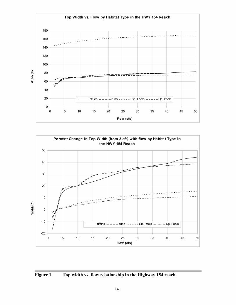
In the Highway 154 reach, the greatest change in top width occurred when flow increasedfrom 1.5 to 5 cfs (Figure 1). This change in flow resulted in a change in top width of 10and 9 feet in run and riffle habitats, respectively (Table 2a), or a relative change of nearly20 and 15 percent, respectively (Table 2b). The top width of shallow pools changed themost as flows went from 5 to 10 cfs (5 feet, 3 percent), while the top width of deep poolschanged the most as flows went from 1.5 to 3 cfs (5 feet, 7 percent). As flows increasedbeyond 15 cfs, the relative change in the top width of all habitats was generally less than3 feet (3 percent) between subsequent flow intervals. Top width increased by between 8and 25 feet (11 and 45 percent), as flow was increased from 3 to 50 cfs, a sixteen-foldincrease in flow. This increase was least in deep pools, which likely provide the besthabitat for steelhead. Riffles and runs had the greatest cumulative increase in habitat, asindicated by greater top width values.

3-2

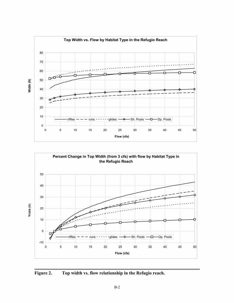
In the Refugio reach, the absolute change in top width from one flow value to the nextexceed 4 feet only for riffle habitats as flow changed from 5 to 10 cfs (Figure 2,Table 2c). This flow interval had the greatest change in top width for all sampledhabitats (Table 2c). These changes ranged from 1.3 to 4.3 feet (Table 2c) or 2 to 9percent (Table 2d). As flow increased above 15 cfs, the relative increase in top widthbetween subsequent flow intervals was generally less than 2 feet (4 percent) for allhabitat types, with the relative change diminishing with increasing flow (Table 2d). Thecumulative percent change in top width as flow increased from 3 to 50 cfs ranged from 5feet (8 percent) in deep pools to 19 feet (43 percent) in riffles (Figure 2).

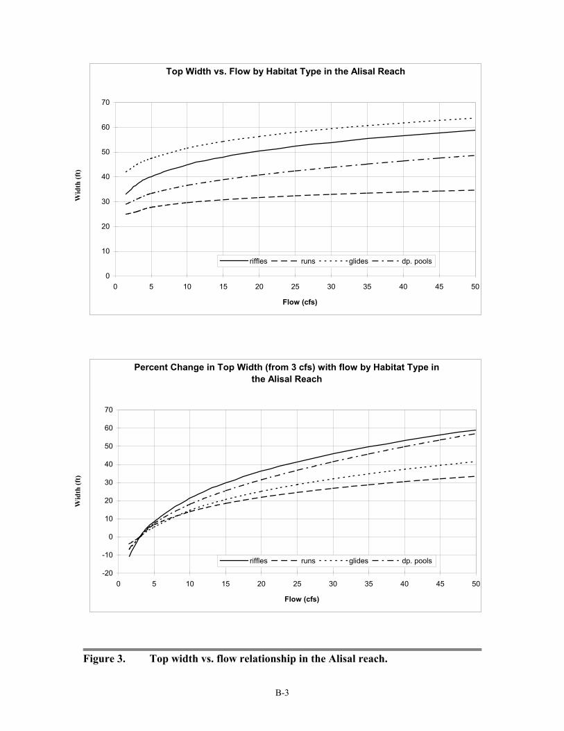
In the Alisal reach, top widths were less than in the Refugio reach for all habitat typesexcept runs (Figure 3). The absolute magnitude of change in top width from one flow tothe next is very similar to that for the Refugio reach, with the greatest changes occurringbetween 5 and 10 cfs for all habitat types (Table 2e). At this flow, top widths changed bybetween 2 and 5 feet depending on habitat. Because the top widths were generally lessthan in the Refugio reach, however, the relative change in top width was somewhathigher, with all habitat types except runs having relative changes in top width of 7 to 12percent (Table 2f) as flow increased from 5 to 10 cfs. As in the other two reaches, therelative change in top width decreases with increasing flow, generally increasing lessthan 3 feet (5 percent) between simulation flows as flow increased beyond 15 cfs. Thecumulative change in top width ranged from 9 to 22 feet (34 to 58 percent) as flowincreased from 3 to 50 cfs (Figure 3). Unlike the other two reaches, deep pools in theAlisal reach had the second highest proportional increase in top width, rather than thelowest increase.

In general, deep pools had the least change in top width in response to changing flows,while riffles had the most change. In the Alisal reach, however, deep pools changedmore than did glides or runs. In all three reaches, the amount of increased flow needed toobtain a given increase in top width is proportionately much greater than the amount ofhabitat gained. For example, to increase glide top widths by 10 percent in the Refugioreach requires more than a 300 percent increase in flow. To attain a similar increase indeep pool habitats in the Highway 154 reach requires an increase in flow of nearly 1,300percent. The habitats in the Alisal reach are more responsive than in the other reaches,requiring about a 200 to 250 percent change in flow to obtain a 10 percent change in topwidth for all habitat types.

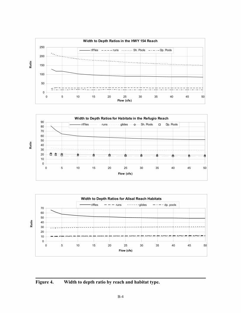
3.2 WIDTH TO DEPTH RATIOS

The width to depth ratios were fairly uniform across the range of flows modeled in allhabitat types except riffles (Figure 4). The width to depth ratio in riffles was generallymuch higher than that of the other habitat types and decreased as flow increased. Therate of change in the width to depth ratios in riffles at the Refugio and Alisal reacheschanged substantially at about 5 cfs. Glides in the Refugio reach and shallow pools inthe other two reaches also had higher width to depth ratios than runs and deep pools. Inthe Highway 154 reach, the width to depth ratios of shallow pools was greater than thatof riffles at all flows and generally declined as flow increased. The declining width to

3-3

depth ratio here and in the riffle habitats in all reaches indicates that the proportionalincrease in width is less than the proportional increase in depth as flow increases. Thisindicates that in these shallow habitat types, habitat is generally improved as flow isincreased, and that this improvement is greatest as flows increase between 1.5 and 5 cfsin the Refugio and Alisal reaches. In the Highway 154 reach, the inflection in the widthto depth ratio is not as pronounced for the riffle or the shallow pool habitats, but appearsto lie between 10 and 15 cfs.

The relatively constant width to depth ratios in the other habitat types indicates that thereis not a substantial change in habitat as flow increases. Based on this, it is reasonable touse the results of the top width analysis to assess changes in habitat with flow in thesehabitats.

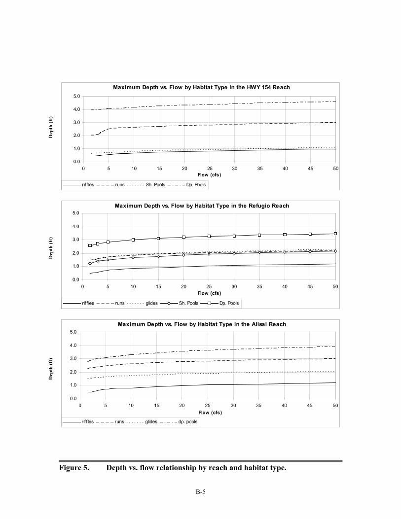
3.3 MAXIMUM DEPTH

As would be expected, the values of maximum depth increased with flow in all reachesand in all habitat types (Table 3, Figure 5). Unexpectedly, deep pools showed an initiallygreater response to changes in flow in the Refugio (Figure 5) and Alisal reaches (Figure5) than did the other habitat types. This greater change in maximum depth is attributed tothe narrower channel widths of deep pools and their inability to increase velocities asrapidly as other habitat types, because of their downstream controls. However, over theentire range of flows simulated, deep pools had the lowest response of any habitat type.Across all sampled habitats, the Refugio reach had the greatest average change in depth(0.8 feet), and the Highway 154 reach had the least (0.6 feet). Generally, depthsincreased relatively slowly over the range of simulated flows in all reaches and in allhabitats. The changes in depth at flows of 1.5 vs. 50 cfs ranged from 0.4 to 1.1 feet forall three reaches and habitats. This 3200 percent increase in flow resulted in an increaseof depth ranging from 15 to 250 percent.

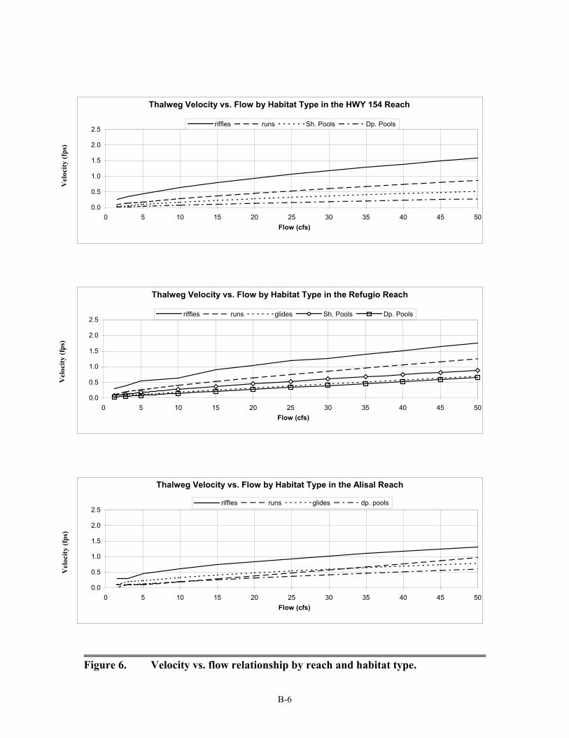
3.4 VELOCITY AT THE THALWEG

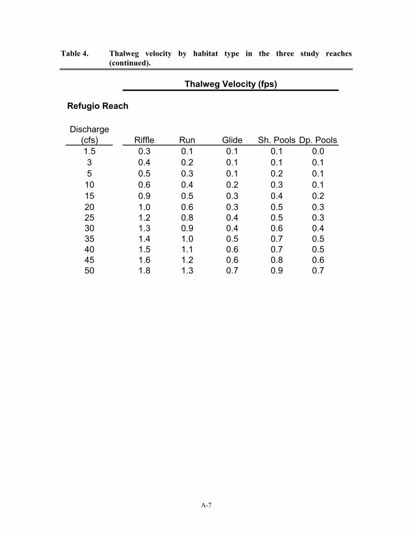
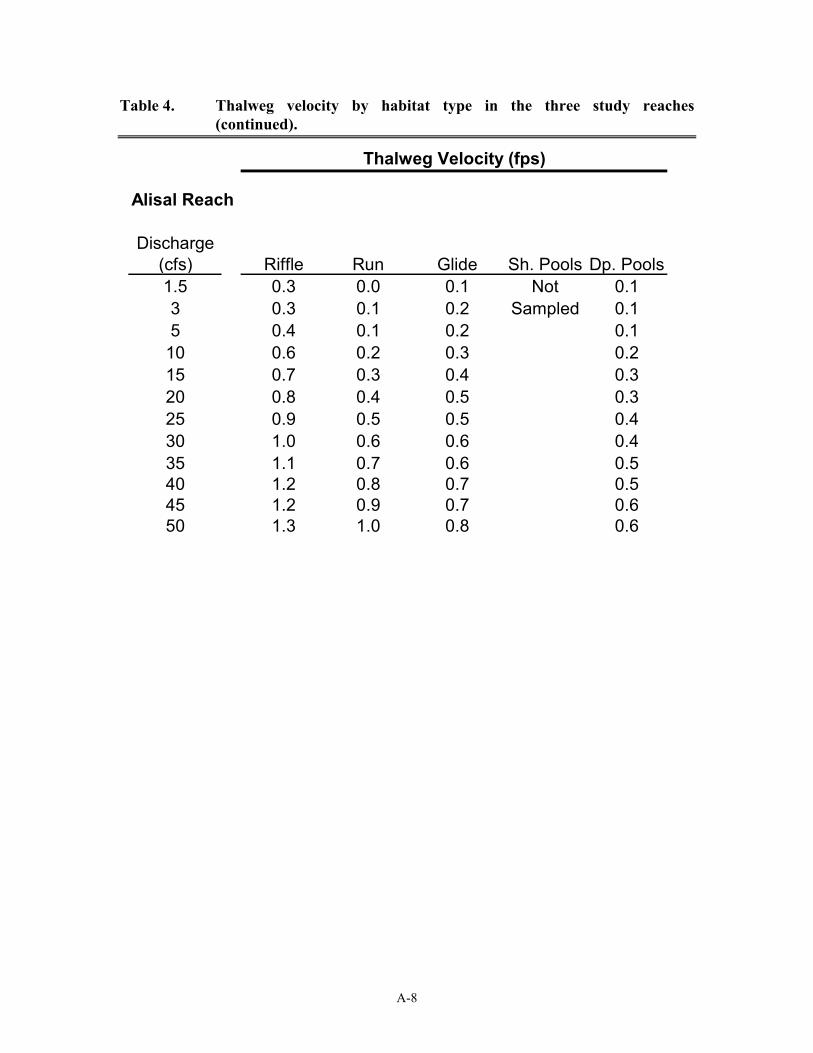
Velocity at the thalweg increased as a function of flow in all habitat types and in allreaches. Riffles had the greatest increase in velocity with increased flow, followed byruns, and then by shallow pools and glides (Table 4, Figure 6). Deep pools had thelowest increase in velocity with increased flow levels. The velocity in riffles at 5 cfs was0.4 to 0.5 fps and increased to 1.3 to 1.8 fps at 50 cfs. In deep pools, velocities were 0.0to 0.1 fps at 5 cfs and 0.3 to 0.7 fps at 50 cfs, depending on the reach.

4-1

4.0CONCLUSIONS

Habitat availability and quality changes with respect to flow were analyzed in themainstem Santa Ynez River below Bradbury Dam. Four types of analyses were utilizedto accomplish this: 1) top width, 2) width to depth ratio, 3) maximum depth, and 4)velocity at the thalweg.

Generally, top width increased most rapidly with flow between 1.5 and 5 cfs for allhabitat types and in all three reaches studied. The top width of riffles tended to increasethe most as flow increased, while deep pools had the least change in top width with flow,with the exception of deep pools in the Alisal reach (which changed more than glides orruns). Top width increased between 5 and 12 feet (equating to top widths of 33 to 66feet) as flow increased from 1.5 and 5 cfs in riffle habitats of all sampled reaches. Asflow increased from 1.5 and 5 cfs in deep pools of all sampled reaches, top widthincreased between 2 and 5 feet (equating to top widths of 29 to 69 feet). In all threereaches studied, the amount of flow required to obtain a given increase in top width wasproportionately much greater than the amount of habitat gained. This is illustrated by theminor changes in top width observed in all habitat types once flow increased beyond 10cfs.

Analysis of width to depth ratios revealed that in most habitat types, there was not asubstantial change in habitat improvement as flow increased, as indicated by relativelyconstant width to depth ratios. However, in shallow habitat types, it was deduced thathabitat generally improves as flow increases, as illustrated by declining width to depthratios with the increase in flow. This improvement was greatest as flows increasedbetween 1.5 and 5 cfs in the Refugio and Alisal reaches. In the Highway 154 reach, theinflection in the width to depth ratio was not as pronounced for the riffle or the shallowpool habitats, but appeared to be between 10 and 15 cfs (Figure 4).

Maximum depth increased with flow in all reaches and habitat types, although depthsgenerally increased relatively slowly over the range of simulated flows. At flows of 1.5cfs and 50 cfs, the changes in depth ranged from 0.4 to 1.1 feet. Deep pools in theRefugio and Alisal reaches showed an initially greater response to changes in flow thandid the other habitat types. This greater response is attributed to the narrower channelwidths of deep pools and the inability to increase velocities as rapidly as other habitattypes due to downstream controls. However, over the entire range of flows simulated,deep pools had the lowest response of any habitat type.

In all habitat types and reaches, velocity at the thalweg increased as a function of flow, asanticipated. The largest increase in velocity with increased flow (from 1.5 to 50 cfs) wasobserved in riffles (0.3 to 1.8 fps), followed by runs (0.0 to 1.3 fps), and then by shallowpools (0.0 to 0.9 fps) and glides (0.1 to 0.8 fps) of all three reaches studied. Deep pools

4-2

had the lowest increase in velocity with increased flow levels (0.0 to 0.7 fps) in all threereaches. Velocities in the Refugio reach were generally the greatest among all threereaches studied.

5-1

5.0LITERATURE CITED

Annear, T. C. and A. L. Conder. 1983. Evaluation of instream flow needs for use inWyoming. Wyoming Game and Fish Department, Fish Division. Completionreport for Contract No. YA-512-CT9-226. 247 pp.

California Department of Water Resources, 1989. Draft Santa Ynez River Instream FlowNeeds Study. CDWR, Red Bluff, CA. 28 pp. and Appendices.

ENTRIX. 1995. Fish resources technical report for the EIS/EIR, Cachuma ProjectContract Renewal. December 5, 1995. Prepared for Woodward-ClydeConsultants.

Nelson, F. A. 1984, unpubl. Guidelines for using the wetted perimeter computerprogram of the Montana Department of Fish, Wildlife and Parks. 104 pp.

Santa Ynez River Technical Advisory Committee (SYRTAC). 1994. CompilationReport for 1994 Santa Ynez River Memorandum of Understanding. Prepared forSanta Ynez River Consensus Committee, Santa Barbara, CA.

Santa Ynez River Technical Advisory Committee (SYRTAC). 1995. CompilationReport for 1995 Santa Ynez River Memorandum of Understanding. Prepared forSanta Ynez River Consensus Committee, Santa Barbara, CA.

Santa Ynez River Technical Advisory Committee (SYRTAC). 1996. ProposedInvestigations to Determine Fish-Habitat Management Alternatives for the LowerSanta Ynez River, Santa Barbara County. March 1996.

Santa Ynez River Technical Advisory Committee (SYRTAC) Biological Subcommittee.1997. Proposed Investigations to Determine Fish-Habitat ManagementAlternatives for the Lower Santa Ynez River, Santa Barbara County: 1997Update. June 1997.

Swift, C. H. 1976. Estimation of stream discharges preferred by steelhead trout forspawning and rearing in western Washington. US Geological Survey Open FileReport 75-155. USGS, Tacoma, WA. 50 pp.

APPENDIX A

TABLES

A-1

Table 1. Top width by habitat type in the three study reaches.

Top Width (ft)Highway 154

Discharge (cfs) Riffle Run Glide Sh. Pools Dp. Pools1.5 54 49 Not 145 643 58 58 Sampled 147 685 66 69 150 69

10 69 70 155 7115 71 75 159 7320 74 77 162 7425 76 78 164 7530 78 79 166 7535 79 80 167 7540 80 80 169 7645 82 81 170 7650 83 81 171 76

Refugio Reach

Discharge (cfs) Riffle Run Glide Sh. Pools Dp. Pools1.5 41 25 51 29 523 44 27 54 30 535 46 28 56 32 54

10 51 30 59 34 5515 53 32 61 36 5620 56 33 62 37 5725 57 33 64 37 5730 59 34 65 38 5735 60 35 65 39 5840 61 36 66 39 5845 62 36 67 40 5850 63 37 68 40 58

Alisal Reach

Discharge (cfs) Riffle Run Glide Sh. Pools Dp. Pools1.5 33 25 42 Not 293 37 26 45 Sampled 315 40 28 47 33

10 45 30 52 3715 48 31 54 3920 50 32 56 4125 52 32 58 4230 54 33 59 4435 55 33 61 4540 57 34 62 4645 58 34 63 4850 59 35 64 49

A-2

Table 2. Change on top width in each reach.

HWY 154

a) b)

Discharge Riffles Runs Glides Sh. Pools Dp. Pools Discharge Riffles Runs Glides Sh. Pools Dp. Pools1.5 - - not - - 1.5 - - not - -3 3.4 9.6 sampled 2.9 4.7 3 6.3 19.6 sampled 2.0 7.45 8.7 10.3 2.7 1.0 5 15.1 17.6 1.8 1.5

10 2.9 1.8 5.2 1.8 10 4.4 2.6 3.5 2.515 2.1 4.6 3.9 1.3 15 3.0 6.6 2.5 1.920 2.4 1.5 3.1 1.3 20 3.4 2.0 1.9 1.725 2.3 1.1 2.0 0.9 25 3.1 1.4 1.2 1.230 1.8 1.5 1.6 0.3 30 2.4 2.0 1.0 0.535 1.3 0.5 1.4 0.3 35 1.7 0.6 0.8 0.440 1.2 0.5 1.2 0.4 40 1.5 0.6 0.7 0.545 2.1 0.4 1.2 0.3 45 2.6 0.5 0.7 0.450 1.1 0.4 1.1 0.2 50 1.3 0.5 0.6 0.3

Change in Top Width (in ft) from Previous Simulated Flow Percent Change in Top Width from Previous Simulated Flow

A-3

Table 2. Change on top width in each reach (continued).

Refugio

c) d)

Discharge Riffles Runs Glides Sh. Pools Dp. Pools Discharge Riffles Runs Glides Sh. Pools Dp. Pools1.5 - - - - - 1.5 - - - - -3 3.0 2.0 3.0 1.9 1.2 3 7.3 8.0 5.9 6.6 2.35 2.5 1.0 1.9 1.5 0.9 5 5.6 3.6 3.5 4.9 1.7

10 4.3 2.1 3.0 2.2 1.3 10 9.2 7.6 5.4 6.9 2.415 2.8 1.4 1.9 1.4 0.8 15 5.4 4.7 3.3 4.1 1.420 2.1 1.1 1.5 1.0 0.6 20 3.9 3.4 2.4 2.9 1.025 1.7 0.9 1.2 0.8 0.5 25 3.0 2.7 1.9 2.3 0.830 1.4 0.8 1.0 0.7 0.4 30 2.5 2.3 1.6 1.9 0.735 1.3 0.7 0.9 0.6 0.3 35 2.1 2.0 1.3 1.6 0.640 1.1 0.6 0.8 0.5 0.3 40 1.9 1.7 1.2 1.4 0.545 1.0 0.5 0.7 0.5 0.2 45 1.7 1.5 1.1 1.2 0.450 0.9 0.5 0.6 0.4 0.2 50 1.5 1.4 0.9 1.1 0.4

Change in Top Width (in ft) from Previous Simulated Flow Percent Change in Top Width from Previous Simulated Flow

A-4

Table 2. Change on top width in each reach (continued).

Alisal

e) f)

Discharge Riffles Runs Glides Sh. Pools Dp. Pools Discharge Riffles Runs Glides Sh. Pools Dp. Pools1.5 - - - not - 1.5 - - - not -3 4.0 1.0 3.0 sampled 2.0 3 12.1 4.0 7.1 sampled 6.95 3.2 1.7 2.5 2.4 5 8.6 6.7 5.5 7.6

10 4.8 1.9 4.1 3.2 10 11.9 6.8 8.7 9.715 3.1 1.2 2.7 2.3 15 6.9 4.0 5.2 6.320 2.4 0.9 2.0 1.9 20 4.9 2.8 3.8 4.825 1.9 0.7 1.7 1.6 25 3.8 2.2 3.0 4.030 1.6 0.6 1.4 1.5 30 3.1 1.8 2.5 3.435 1.4 0.5 1.2 1.3 35 2.6 1.5 2.1 3.040 1.3 0.4 1.1 1.2 40 2.3 1.3 1.8 2.745 1.2 0.4 1.0 1.2 45 2.0 1.2 1.6 2.550 1.1 0.4 0.9 1.1 50 1.8 1.1 1.5 2.3

Change in Top Width (in ft) from Previous Simulated Flow Percent Change in Top Width from Previous Simulated Flow

A-5

Table 3. Thalweg depth by habitat type in the three study reaches.

Maximum Depth (ft)

Highway 154Discharge (cfs) Riffle Run Glide Sh. Pools Dp. Pools

1.5 0.4 2.1 Not 0.7 4.03 0.5 2.1 Sampled 0.7 4.15 0.6 2.5 0.8 4.1

10 0.7 2.7 0.8 4.215 0.7 2.7 0.9 4.320 0.8 2.8 0.9 4.425 0.8 2.9 1.0 4.430 0.9 2.9 1.0 4.535 0.9 2.9 1.0 4.540 0.9 3.0 1.1 4.645 1.0 3.0 1.1 4.650 1.0 3.0 1.1 4.6

Refugio ReachDischarge (cfs) Riffle Run Glide Sh. Pools Dp. Pools

1.5 0.5 1.5 1.5 1.3 2.63 0.6 1.6 1.6 1.4 2.75 0.7 1.7 1.7 1.5 2.8

10 0.8 1.9 1.9 1.7 3.015 0.9 2.0 2.0 1.8 3.120 1.0 2.0 2.1 1.9 3.225 1.0 2.1 2.1 1.9 3.330 1.1 2.1 2.2 2.0 3.335 1.1 2.1 2.2 2.0 3.440 1.1 2.2 2.2 2.1 3.445 1.2 2.2 2.3 2.1 3.450 1.2 2.2 2.3 2.2 3.5

Alisal ReachDischarge (cfs) Riffle Run Glide Sh. Pools Dp. Pools

1.5 0.5 2.3 1.5 Not 2.83 0.6 2.4 1.6 Sampled 3.05 0.7 2.5 1.7 3.1

10 0.8 2.6 1.8 3.315 0.9 2.7 1.8 3.520 1.0 2.8 1.9 3.625 1.0 2.9 1.9 3.730 1.1 2.9 2.0 3.735 1.1 2.9 2.0 3.840 1.2 3.0 2.0 3.845 1.2 3.0 2.0 3.950 1.2 3.0 2.1 3.9

A-6

Table 4. Thalweg velocity by habitat type in the three study reaches.

Thalweg Velocity (fps)

Highway 154

Discharge (cfs) Riffle Run Glide Sh. Pools Dp. Pools1.5 0.3 0.1 Not 0.0 0.03 0.4 0.1 Sampled 0.1 0.05 0.4 0.2 0.1 0.0

10 0.6 0.3 0.2 0.115 0.8 0.4 0.2 0.120 0.9 0.5 0.3 0.125 1.1 0.5 0.3 0.230 1.2 0.6 0.4 0.235 1.3 0.7 0.4 0.240 1.4 0.7 0.5 0.245 1.5 0.8 0.5 0.350 1.6 0.9 0.5 0.3

A-7

Table 4. Thalweg velocity by habitat type in the three study reaches(continued).

Thalweg Velocity (fps)

Refugio Reach

Discharge (cfs) Riffle Run Glide Sh. Pools Dp. Pools1.5 0.3 0.1 0.1 0.1 0.03 0.4 0.2 0.1 0.1 0.15 0.5 0.3 0.1 0.2 0.1

10 0.6 0.4 0.2 0.3 0.115 0.9 0.5 0.3 0.4 0.220 1.0 0.6 0.3 0.5 0.325 1.2 0.8 0.4 0.5 0.330 1.3 0.9 0.4 0.6 0.435 1.4 1.0 0.5 0.7 0.540 1.5 1.1 0.6 0.7 0.545 1.6 1.2 0.6 0.8 0.650 1.8 1.3 0.7 0.9 0.7

A-8

Table 4. Thalweg velocity by habitat type in the three study reaches(continued).

Thalweg Velocity (fps)

Alisal Reach

Discharge (cfs) Riffle Run Glide Sh. Pools Dp. Pools1.5 0.3 0.0 0.1 Not 0.13 0.3 0.1 0.2 Sampled 0.15 0.4 0.1 0.2 0.1

10 0.6 0.2 0.3 0.215 0.7 0.3 0.4 0.320 0.8 0.4 0.5 0.325 0.9 0.5 0.5 0.430 1.0 0.6 0.6 0.435 1.1 0.7 0.6 0.540 1.2 0.8 0.7 0.545 1.2 0.9 0.7 0.650 1.3 1.0 0.8 0.6

APPENDIX B

FIGURES

B-1

Figure 1. Top width vs. flow relationship in the Highway 154 reach.

Wid

th (f

t)W

idth

(ft)

Top Width vs. Flow by Habitat Type in the HWY 154 Reach

0

20

40

60

80

100

120

140

160

180

0 5 10 15 20 25 30 35 40 45 50

Flow (cfs)

rif f les runs Sh. Pools Dp. Pools

Percent Change in Top Width (from 3 cfs) with flow by Habitat Type in the HWY 154 Reach

-20

-10

0

10

20

30

40

50

0 5 10 15 20 25 30 35 40 45 50Flow (cfs)

rif f les runs Sh. Pools Dp. Pools

B-2

Figure 2. Top width vs. flow relationship in the Refugio reach.

Top Width vs. Flow by Habitat Type in the Refugio Reach

0

10

20

30

40

50

60

70

80

0 5 10 15 20 25 30 35 40 45 50

Flow (cfs)

riffles runs glides Sh. Pools Dp. Pools

Percent Change in Top Width (from 3 cfs) with flow by Habitat Type in the Refugio Reach

-10

0

10

20

30

40

50

0 5 10 15 20 25 30 35 40 45 50

Flow (cfs)

riffles runs glides Sh. Pools Dp. Pools

Wid

th (f

t)W

idth

(ft)

B-3

Figure 3. Top width vs. flow relationship in the Alisal reach.

Top Width vs. Flow by Habitat Type in the Alisal Reach

0

10

20

30

40

50

60

70

0 5 10 15 20 25 30 35 40 45 50

Flow (cfs)

riffles runs glides dp. pools

Percent Change in Top Width (from 3 cfs) with flow by Habitat Type in the Alisal Reach

-20

-10

0

10

20

30

40

50

60

70

0 5 10 15 20 25 30 35 40 45 50

Flow (cfs)

riffles runs glides dp. pools

Wid

th (f

t)W

idth

(ft)

B-4

Figure 4. Width to depth ratio by reach and habitat type.

Width to Depth Ratios for Alisal Reach Habitats

010203040506070

0 5 10 15 20 25 30 35 40 45 50

Flow (cfs)

riffles runs glides dp. pools

Rat

ioR

atio

Rat

io

Width to Depth Ratios in the HWY 154 Reach

0

50

100

150

200

250

0 5 10 15 20 25 30 35 40 45 50Flow (cfs)

rif f les runs Sh. Pools Dp. Pools

Width to Depth Ratios for Habitats in the Refugio Reach

0102030405060708090

0 5 10 15 20 25 30 35 40 45 50

Flow (cfs)

rif f les runs glides Sh. Pools Dp. Pools

B-5

Figure 5. Depth vs. flow relationship by reach and habitat type.

Maximum Depth vs. Flow by Habitat Type in the HWY 154 Reach

0.0

1.0

2.0

3.0

4.0

5.0

0 5 10 15 20 25 30 35 40 45 50Flow (cfs)

rif f les runs Sh. Pools Dp. Pools

Maximum Depth vs. Flow by Habitat Type in the Refugio Reach

0.0

1.0

2.0

3.0

4.0

5.0

0 5 10 15 20 25 30 35 40 45 50Flow (cfs)

rif f les runs glides Sh. Pools Dp. Pools

Maximum Depth vs. Flow by Habitat Type in the Alisal Reach

0.0

1.0

2.0

3.0

4.0

5.0

0 5 10 15 20 25 30 35 40 45 50Flow (cfs)

rif f les runs glides dp. pools

Dep

th (f

t)D

epth

(ft)

Dep

th (f

t)

B-6

Figure 6. Velocity vs. flow relationship by reach and habitat type.

Thalweg Velocity vs. Flow by Habitat Type in the HWY 154 Reach

0.0

0.5

1.0

1.5

2.0

2.5

0 5 10 15 20 25 30 35 40 45 50Flow (cfs)

riffles runs Sh. Pools Dp. Pools

Thalweg Velocity vs. Flow by Habitat Type in the Refugio Reach

0.0

0.5

1.0

1.5

2.0

2.5

0 5 10 15 20 25 30 35 40 45 50Flow (cfs)

riffles runs glides Sh. Pools Dp. Pools

Thalweg Velocity vs. Flow by Habitat Type in the Alisal Reach

0.0

0.5

1.0

1.5

2.0

2.5

0 5 10 15 20 25 30 35 40 45 50Flow (cfs)

riffles runs glides dp. pools

Vel

ocity

(fps

)V

eloc

ity (f

ps)

Vel

ocity

(fps

)