1

Minnesota Department of Natural Resources Investigational Report 539, December 2006

SUMMER HABITAT ASSOCIATIONS OF LARGE BROWN TROUT

IN SOUTHEAST MINNESOTA STREAMS1

Douglas J. Dieterman, William C. Thorn, Charles S. Anderson, and Jeffrey L. Weiss

(corresponding author: douglas.dieterman@dnr.state.mn.us)

Minnesota Department of Natural Resources

Division of Fish and Wildlife 500 Lafayette Road

St. Paul, MN 55155-4020

Abstract.--We evaluated summer habitat use of large brown trout Salmo trutta (TL > 380 mm) in pools and stream reaches of southeast Minnesota to test an earlier summer habitat model, to identify other important variables, and to develop a habitat quality classification to guide large trout management. We collected 224 large trout in 126 of 581 pools in 41 stream reaches during 2003 and 2004. The probability (P2) that a large brown trout was present in a pool was positively associated with the pres-ence of water deeper than 90 cm, instream rock, overhead bank cover, and woody de-bris in a logistic regression model. Similarly, large trout abundance in pools was best predicted with a Poisson regression model with four variables (area of water deeper than 60 cm, length of overhead bank cover, pool width, and area of instream rock). Streambank riprap was not significantly associated with either large trout presence or abundance in pools. Large trout abundance in stream reaches increased linearly with mean P2-value, which explained 54% of the variation among study reaches. We cate-gorized habitat quality of stream reaches into four classes based on mean P2-values. In large streams (>0.43 m3/s), with poor to fair habitat quality, habitat management should increase water deeper than 90 cm, instream rock, overhead bank cover, and woody debris. Habitat management for large trout in smaller streams (<0.43 m3/s) is more complex and may simply be more limited. Managers may have to recognize the limited biological potential in these systems and prioritize large trout management ob-jectives to larger streams.

1 This project was funded in part by the Federal Aid in Sport Fish Restoration (Dingell-Johnson) program. Completion Report, Study 667, D-J Project F-26-R, Minnesota.

2

Introduction

Large brown trout Salmo trutta (TL > 380 mm) are of high value to some anglers who request specific management actions to produce greater abundance and catch of large trout. Managers know that mean abundance of adult trout in southeast Minnesota streams increased from 139/km during 1970-1979 to 702/km during 1991-2001 (405%), and that mean abundance of large trout increased from 3/km to 6/km (100%; Thorn et al. in review). However, some anglers are convinced that abundance of large trout declined, perhaps because the proportion of large trout caught had declined or the slower rate of increase for large trout was less noticeable. This discrep-ancy has lead to requests for more protective fishing regulations and special habitat rehabili-tation features. The success or failure of man-agement actions may depend on the abundance of high quality habitat for large trout within a stream reach. For example, spe-cial regulations to reduce angling mortality may not produce more large trout if habitat quality is poor.

Large brown trout move through streams seasonally and select pools with ap-propriate habitat. Large brown trout often move extensively during spring and fall, but are relatively sedentary, using small home ar-eas, often limited to a single pool, during win-ter and summer (Bachman 1984; Clapp et al. 1990; Meyers et al. 1992; Burrell et al. 2000). Seasonal movements are likely due to spawn-ing migrations and movement between winter and summer habitats. During summer, large brown trout often select the deepest pools with abundant cover, especially overhead cover (Heggenes 1988; Greenberg et al. 2001; Diana et al. 2004). Pool depth and an abundance of complex covers, such as woody debris and undercut banks, are believed to provide more energetically profitable stream positions due to velocity reductions, decrease intraspecific competition through visual isolation, and pro-vide protection from avian and mammalian predators (Bjornn and Reiser 1991; Sundbaum and Näslund 1998; Greenberg et al. 2001). Although some brown trout exhibit nighttime foraging movements through multiple pools, typically returning to daytime resting locations

near cover in their original pool (Clapp et al. 1990; Diana et al. 2004), other brown trout exhibit a complete absence of diel movement during summer (Bunnell et al. 1998).

To evaluate the potential of a stream for large trout management in southeast Min-nesota, fisheries biologists investigated trout abundance, growth potential, habitat quality, and trout harvest (MNDNR 2000). Biologists have estimated abundance in most streams and evaluated factors related to growth potential (Dieterman et al. 2004). Evaluations of habi-tat quality and harvest of large trout from standard creel surveys, however, are less cer-tain. A standardized method of measuring and classifying habitat quality for large brown trout may enable fish managers to identify streams where instream habitat improvement or regulations would be most likely to suc-ceed. Development of such a habitat quality classification first requires identification of habitat features used by large brown trout.

A pool-scale habitat model and subse-quent reach-scale habitat quality classification for large brown trout were proposed for south-east Minnesota (Thorn and Anderson 1993; Thorn and Anderson 2001a), but rigorous test-ing of such models is required for confident management application (Rabeni 1992). Thorn and Anderson (1993) determined im-portant habitat features influencing pres-ence/absence (P/A) of large brown trout in pools in southeast Minnesota streams. They found that the probability (P-value) of finding a large brown trout in a pool was positively related to the presence of water deeper than 60 cm and presence of four cover types: woody debris, instream rock, overhead bank cover, and stream bank riprap. As more cover types were added to a pool, the probability a large trout would be present increased. Thorn and Anderson (2001a) recommended using quar-tiles based on P-values (as summarized in Ta-ble 8 of Thorn and Anderson 1993), to classify habitat quality in stream reaches as poor, fair, good, or excellent for large brown trout. First, each pool in the reach is assigned a P-value based on Table 8 in Thorn and Anderson (1993). Then the quartile (<0.25, 0.25 – 0.49, 0.50 – 0.74, >0.75) with the largest number of pools (i.e., mode) and the overall mean P-value for all pools were used to determine the

3

habitat quality class for the reach. For exam-ple, habitat quality of Diamond Creek was classified as good because the P-value for 61% of the pools in the reach and the mean P (0.55) for all pools in the reach were both in the third quartile. However, J. Weiss (personal obser-vation) found little agreement with the mean and modal P-values for 721 pools in 13 stream reaches. Although adding cover to a pool typically increased the P-value, several com-binations of cover types when added to an-other specific cover type reduced the estimated probability (see Table 8 in Thorn and Anderson 1993). Because such negative interactions seem unlikely, it is assumed that some model terms were poorly estimated due to sampling noise or collinearity problems in the initial study.

To verify the importance of the habitat features originally determined by Thorn and Anderson (1993), we applied their earlier P/A model to an independent dataset. We devel-oped new models relating habitat features to large brown trout P/A and abundance in pools, and abundance in stream reaches. From these results, we developed a revised reach-scale habitat quality classification to guide man-agement for large brown trout in southeast Minnesota streams (MNDNR 2000). The goal of this revised classification is to classify habi-tat in stream reaches into poor, fair, good or excellent habitat classes, and then relate these categories to large trout abundance. Specific objectives were to: (1) test the original pool-scale P/A model of Thorn and Anderson (1993) with an independent data set; (2) de-velop a new pool-scale P/A model with a newer and larger dataset; (3) develop a pool-scale large trout abundance model; (4) develop a reach-scale large trout abundance model; and (5) develop a habitat quality classification and relate these classes to large trout abun-dance.

Methods

We selected 41 study stations within

stream reaches that represented the range of physical habitat conditions for southeast Min-nesota trout streams. Study stations were as-sumed to represent stream reach conditions and are hereafter referred to simply as reaches.

Study reaches usually included 10-15 pools, and no more than 25% of reaches had instream habitat that had been rehabilitated since 1970. Although channel morphology of these streams varied, separate pools were easily identified in most streams by riffles between them. A few pools were delineated by a re-duction in depth, not by coarse substrate. We sampled from mid-July through the first week in October in 2003 and 2004. Pool-scale

To test the original model of Thorn and Anderson (1993), we estimated large trout abundance and recorded the presence of the same five summer cover variables (overhead bank cover, riprap, instream rocks, woody de-bris, and water deeper than 60 cm) in each pool in 20 study reaches sampled in 2003 and 6 reaches in 2004. We made upstream elec-trofishing passes through each pool until no large trout were captured. The estimate of large trout for the pool was the sum of all large trout captured. In most streams, trout were sampled with a towed electrofishing barge with two or three handheld anodes. In the few pools that were not completely wadable, biologists floated in bellyboats. In one stream, we used two barges and five elec-trodes. In small streams, the sampling gear was one or two backpack electrofishers. Us-ing the instream cover data and Table 8 in Thorn and Anderson (1993), we calculated the P-values (the expected probability of finding at least one large trout) for each pool.

To develop pool-scale P/A and abun-dance models for large brown trout, we also measured the abundance of 13 important summer covers for large trout in each pool for all 20 study reaches sampled in 2003 and for 6 study reaches sampled in 2004. We consid-ered overhead bank cover longer than 0.6 m, deeper than 0.15 m, and wider than 0.3 m would provide cover for large trout. Over-hanging grass was considered overhead bank cover when wider than 0.7 m. We measured overhead bank cover by length (Lobc), area (OBC), and as length of overhead bank cover per thalweg length of each pool (Lobc/T). Crevices in riprap provided cover for large trout. The area of cover from riprap (RR) was calculated by multiplying the length of riprap

4

by either 0.1, 0.25, or 0.5 depending on how many crevices were available above the streambed for cover (0.1 = few crevices), and this value by 0.3 m to represent the average width of riprap extending into stream banks. Hayes and Jowett (1994) found instream rocks that were at least 0.027 m2 in diameter pro-vided cover for drift-feeding brown trout, but when larger boulders were available, brown trout used them almost exclusively. We deemed instream rocks covering areas greater than 0.225 m2 would provide cover for large brown trout in our study streams. Thus, area of cover from instream rocks (IR) was esti-mated in increments of 0.225 m2 (1.5 m long X 0.15 m wide), and summed for each pool. White (1996) reviewed numerous fish habitat studies and concluded that woody debris gen-erally provided cover when larger than 0.20 m2. However, White (1996) acknowledged that larger wood sizes may be necessary to provide cover for larger fishes or in larger stream systems. We considered woody debris to provide cover for large brown trout when it covered an area of stream at least 0.45 m2 and we estimated this cover type (DEB) in incre-ments of this area (1.5 m X 0.3 m). The area of water deeper than 60 cm (D60) was calcu-lated from its length and average width. When more than one deep-water area was present in a pool, each area was measured and all areas were summed for the pool. An alternative used in some larger pools was the placement of transects at regular intervals to record the width of each water depth at each transect, calculating the length of each water depth and average width from transect data, and multi-plying length times mean average width to estimate area. We similarly estimated the area of water deeper than 90 (D90), 120 (D120), and 150 (D150) cm. We also measured thal-weg length (T), width (W), and area (Area) of each pool.

For our first objective, testing the pool-by-pool P/A habitat model of Thorn and Anderson (1993), we first calculated a P-value for each pool based on the presence of four types of cover and water deeper than 60 cm. If this P-value was greater than 0.5 (i.e., greater than a 50% chance that a large trout should be present), we predicted that pool should have a large trout present. If the P-

value was less than 0.5 we predicted that large brown trout should be absent from that pool. Actual P/A of a large brown trout in each pool was determined from electrofishing results. We then compared the predicted P/A to the observed P/A with a classification table and chi-square test of association (Hatcher and Stepanski 1994). A significant chi-square test (P ≤ 0.05) would indicate that the model-predicted data were associated with observed data, indicating an accurate model.

Then, we repeated the logistic regres-sion modeling analysis of Thorn and Anderson (1993), although without the complication of sub-sampling of pools without large trout, to see whether the same habitat variables were important as main effects. Prior to model building, we fit and plotted generalized addi-tive models (GAM; SAS Institute Inc. 2001) for each independent variable to ascertain logit linearity (Hosmer and Lemeshow 1989). If logits were not linear with raw data, we trans-formed variables and reassessed linearity with GAMs. We initially tested the full range of cover variables originally tested by Thorn and Anderson (1993) for significant associations with large trout P/A in pools. However, the D120 and D150 variables were omitted be-cause the coefficients were unstable, likely because of rarity. We used purposeful and stepwise forward approaches to determine the subset of variables and interaction terms to include in the final habitat selection model. For stepwise forward approaches, we used P values chosen to enter and remove variables of 0.15 and 0.20, respectively (Thorn and Ander-son 1993). Models were also evaluated for significance with a log-likelihood test for the overall model; the Wald chi-square statistic, which compares the individual slope coeffi-cients to see if they differ from zero (i.e., no effect); and an adjusted generalized R2 (Hos-mer and Lemeshow 1989; Nagelkerke 1991; Menard 1995).

For our third objective, we developed a pool-scale model relating trout abundance in pools to habitat variables using Poisson re-gression. We started by running a full model with all 13 habitat variables with the general linear modeling procedure in Statistical Analysis Systems software (McCullagh and Nelder 1989). However, the D120 and D150

5

variables were again omitted because of un-stable coefficients. We then assessed the sig-nificance of each habitat variable as a main effect with a chi-square test, and manually removed non-significant variables until we developed a final model (SAS Institute Inc. 1999). The final model was assessed with a goodness-of-fit test for the overall model, a Wald χ2 statistic which tested the significance of individual slope coefficients, and a log-likelihood χ2 statistic comparing one model to another (SAS Institute Inc. 1999).

Reach scale

To develop a reach-scale model of factors associated with large brown trout abundance, our fourth objective, we recorded data for 37 variables from 20 stream reaches in 2003. Although we had initially intended to validate this 2003 reach-scale model with data collected in 2004 (i.e., only those variables necessary to validate the 2003 model), new results prompted development of a revised reach-scale model (see Results below). Con-sequently, all reach-scale variables were not measured for 15 of the 21 reaches sampled in 2004. We measured length, width, mean depth, estimated substrates, and calculated area of each pool and riffle in the reach fol-lowing methods in MNDNR (1978). Trout cover (as described above), pool type, bank erosion, percent aquatic vegetation, and per-cent pool bank shade were also measured or estimated in each pool (MNDNR 1978). We then calculated reach totals or means from these individual pool and riffle measurements (MNDNR 1978). We measured gradient and discharge, calculated the width:depth ratio, recorded sinuosity from the latest stream sur-vey, and calculated stream class (Thorn and Anderson 1999) and habitat quality class (Thorn and Anderson 2001a). Abundance and biomass of smaller trout in the reach was re-corded from previous electrofishing surveys. We included five GIS watershed variables for each reach (drainage basin area, watershed slope, land use, minimum soil permeability, and K factor of the Universal Soil Loss Equa-tion). Minimum soil permeability and the K factor of the Universal Soil Loss Equation are indicators of the susceptibility of soils in the

watershed to erosion (USDA 1991). Large trout abundance in the reach, the dependent variable, was the sum of abundance in all pools in the reach, and converted to density (number per km). We culled reach-scale vari-ables following methods in Dieterman and Galat (2004) because we had more predictor variables, 37, than stream reach replicates (N=20) in 2003. Individual reach-scale vari-ables significantly related (P < 0.05) to abun-dance of large brown trout in reaches were first identified with univariate linear regres-sion models. Variables not significantly re-lated were culled. To reduce problems of collinearity in final multiple model building steps, Pearson’s rank correlations were then used to identify which remaining variables were correlated. Multiple regression models were then developed by manually entering and removing variables until the best model; based on significance, variation explained, and lack of collinearity was achieved.

Habitat Quality Classification

Our fifth objective was to develop a reach-scale habitat quality classification for large brown trout in southeast Minnesota streams. If a reach model relating abundance directly to habitat (i.e., reach-scale mean P-value) was developed, quartiles of mean P-values or other cut points might be used to classify habitat as poor, fair, good, or excel-lent. Our preferred criteria for an adequate reach-scale habitat classification, was that large trout abundance differed significantly among habitat classes. At a minimum, large trout abundance must differ between poor-fair and good-excellent habitat groupings to guide selection of reaches requiring instream habitat rehabilitation following MNDNR (2000). We used trout abundance information from this study as an initial test of abundance differ-ences among our proposed habitat classes, but recognize the tautological nature of using trout abundance data to both develop a reach-scale model and subsequently test for differences among proposed habitat classes from this model. We acknowledge that additional data should be collected to better test our classifica-tions. Finally, extensive habitat degradation in the region (Thorn et al. 1997; Thorn and Anderson 2001a) should result in a proposed

6

classification scheme with few reaches rated as good or excellent habitat if our study reach selection was a true representation of south-east Minnesota streams. We ranked stream reaches from highest to lowest P-value and visually interpreted potential breaks between poor, fair, good, and excellent habitat quality classes. Then we used Kruskal-Wallis and Wilcoxon two-sample tests to test whether large trout abundance differed significantly (P < 0.05) among these proposed habitat classes.

Results

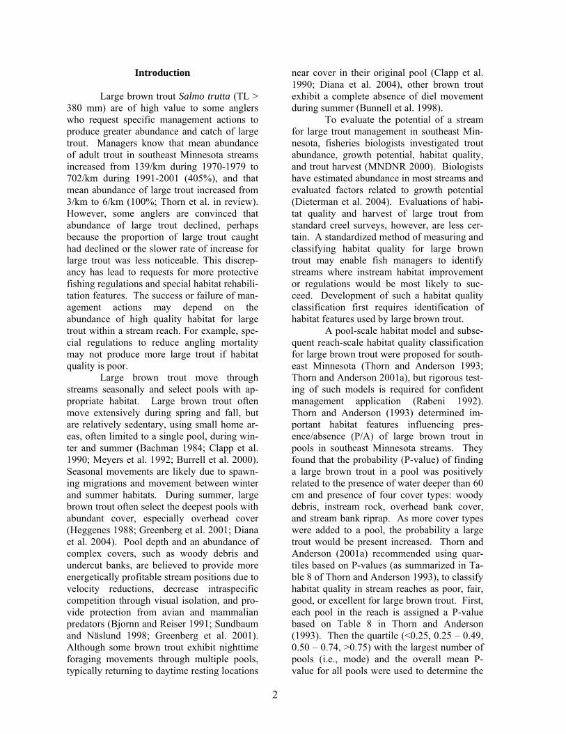
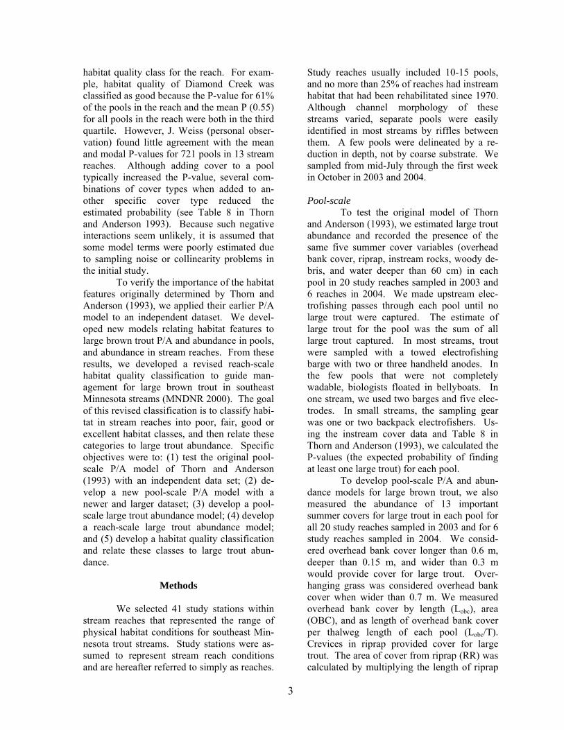
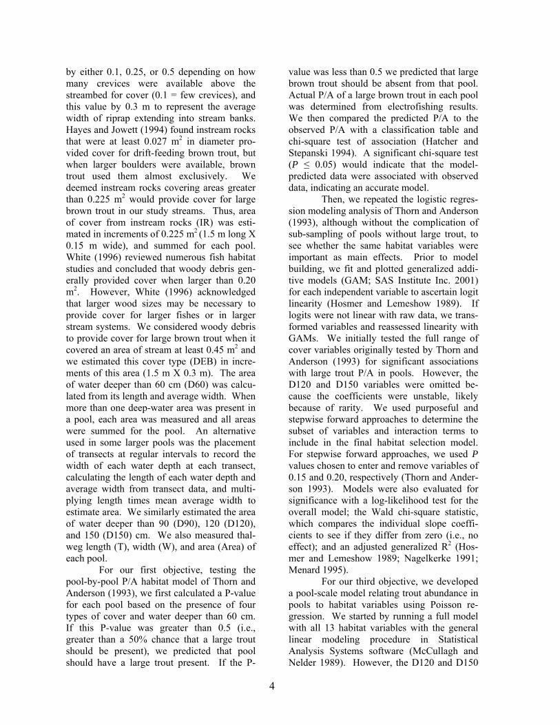
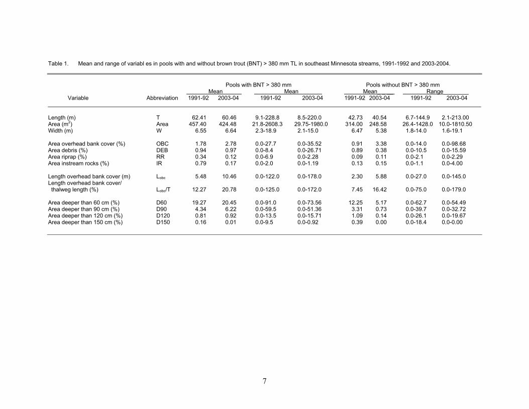
We electrofished 580 pools in 41 stream reaches in 2003 and 2004, and col-lected 224 large brown trout (0.39/pool) from 126 of the pools (22% of pools). Multiple large trout were collected in 46 pools, with a maximum of 11 in one pool. During 1991-1992, Thorn and Anderson (1993), elec-trofished 511 pools in 21 stream reaches and collected 157 trout (0.31/pool) in 107 pools (21% of pools). Multiple large trout were sampled in 28 pools, and the maximum was 6. Our range of values for many habitat variables in 2003 and 2004 was greater than in 1991-1992 (Table 1). We selected streams to represent the range of regional stream condi-tions (Appendix Tables A1-A5), but Thorn and Anderson (1993), selected stream reaches known or expected to contain large trout. For example, the reach of Badger Creek in 2003 was characterized by no riffles, pools distin-guished by thalweg crossover and sand “dunes,” and abundant overhead bank cover from overhanging grass on both stream banks (Lobc/T of 162.3% for the reach). In 1991-1992, such a stream reach was not sampled. Without the Badger Creek data, mean percent-age of overhead bank cover in pools without a large trout would decrease from 3.4% to 2.7%. Also, in pools with large trout, the mean per-centage of pools with riprap was 0.34 in 1991-1992 and 0.12 in 2003-2004 (Table 1). Pool scale The Thorn and Anderson (1993) model based on the presence of five cover variables was informative about the pres-ence/absence of large brown trout in pools in this study (χ2 = 47.63, df = 1, P < 0.001). The

mean P-value for pools with a large trout (0.484) was 43% greater (t- test, P <0.01) than the mean P-value for pools without a large trout (0.276). Overall, the model correctly predicted P/A in 70% of the 580 pools sam-pled (Table 2). However, the model had a high Negative Predictive Value, correctly pre-dicting absence in 333 of 384 pools (87%), and a lower Positive Predictive Value, cor-rectly predicting presence in 75 of 196 pools (38%). In the newer dataset, presence of a large brown trout in a pool was positively as-sociated with the presence of water > 90 cm deep, instream rock, overhead bank cover, and woody debris, with two negative interaction terms (Table 3). All four cover variables in the final model had been transformed to pres-ence/absence values because responses were not linear on the logit scale. The six-term model was significant (log likelihood χ2 = 112.75, df = 6, P < 0.0001), explained 40.8% of the variation in these data, and included some main effects originally identified by Thorn and Anderson (1993) (e.g., woody de-bris and overhead bank cover). Although the interaction terms were negative, they were small relative to the main effects, thus for any set of cover types present, the addition of an-other cover type increased the predicted prob-ability of large trout presence. This avoids a problematic aspect of the Thorn and Anderson (1993) model, where addition of another cover type did not always increase predicted prob-abilities. Some cover types originally included in the Thorn and Anderson (1993) model (e.g., riprap, pool length, and water deeper than 60 cm), were not associated with large trout P/A in these newer data. Area of water deeper than 60 cm was tested in our multiple model development because it was significantly as-sociated with large trout presence in our uni-variate general additive models. However, area of water deeper than 60 cm and the pres-ence/absence of water deeper than 90 cm were nested and highly correlated prompting inclu-sion of only one of these terms. We retained the presence/absence of D90 in our multiple regression model because the model with D60 only explained 28.1% of the variation in these data and provided a poorer fit to the data

7

Table 1. Mean and range of variabl es in pools with and without brown trout (BNT) > 380 mm TL in southeast Minnesota streams, 1991-1992 and 2003-2004. Pools with BNT > 380 mm Pools without BNT > 380 mm Mean Mean Mean_ _ __ Range________ Variable Abbreviation 1991-92 2003-04 1991-92 2003-04 1991-92 2003-04 1991-92 2003-04 Length (m) T 62.41 60.46 9.1-228.8 8.5-220.0 42.73 40.54 6.7-144.9 2.1-213.00 Area (m2) Area 457.40 424.48 21.8-2608.3 29.75-1980.0 314.00 248.58 26.4-1428.0 10.0-1810.50 Width (m) W 6.55 6.64 2.3-18.9 2.1-15.0 6.47 5.38 1.8-14.0 1.6-19.1 Area overhead bank cover (%) OBC 1.78 2.78 0.0-27.7 0.0-35.52 0.91 3.38 0.0-14.0 0.0-98.68 Area debris (%) DEB 0.94 0.97 0.0-8.4 0.0-26.71 0.89 0.38 0.0-10.5 0.0-15.59 Area riprap (%) RR 0.34 0.12 0.0-6.9 0.0-2.28 0.09 0.11 0.0-2.1 0.0-2.29 Area instream rocks (%) IR 0.79 0.17 0.0-2.0 0.0-1.19 0.13 0.15 0.0-1.1 0.0-4.00 Length overhead bank cover (m) Lobc 5.48 10.46 0.0-122.0 0.0-178.0 2.30 5.88 0.0-27.0 0.0-145.0 Length overhead bank cover/ thalweg length (%) Lobc/T 12.27 20.78 0.0-125.0 0.0-172.0 7.45 16.42 0.0-75.0 0.0-179.0 Area deeper than 60 cm (%) D60 19.27 20.45 0.0-91.0 0.0-73.56 12.25 5.17 0.0-62.7 0.0-54.49 Area deeper than 90 cm (%) D90 4.34 6.22 0.0-59.5 0.0-51.36 3.31 0.73 0.0-39.7 0.0-32.72 Area deeper than 120 cm (%) D120 0.81 0.92 0.0-13.5 0.0-15.71 1.09 0.14 0.0-26.1 0.0-19.67 Area deeper than 150 cm (%) D150 0.16 0.01 0.0-9.5 0.0-0.92 0.39 0.00 0.0-18.4 0.0-0.00

8

Table 2. Accuracy of pool-scale logistic regression models developed from 1991-1992 (Thorn and Anderson 1993; Table 8) for predicting presence/absence of large brown trout (> 380 mm TL) in pools in 2003 and 2004, based on presence/absence of five cover variables, in southeast Minnesota streams. For the proportion of pools, the first number is the observed number and the second number is the predicted number. For ex-ample, the first value (75/196) shows that large trout were predicted to be present in 196 pools but were observed present in only 75 of these 196 pools.

Model prediction

Proportion of pools

Percentage of pools

Correct predictions Large trout present where predicted to be present 75/196 38% Large trout absent where predicted to be absent 333/384 87% Incorrect predictions Large trout absent where predicted to be present 121/196 62% Large trout present where predicted to be absent 51/384 13% Overall correct classification 408/580 70% Table 3. Estimated coefficients, standard errors (SE), and Wald χ2-statistic testing for significance of the individual

coefficients for a multiple logistic regression model predicting presence/absence of brown trout > 380 mm TL in southeast Minnesota streams, 2003-2004.

Variable Coefficient SE Wald χ2 P > χ2

Constant -4.097 0.518 62.39 <0.0001 OBC (0=absent, 1=present) 1.616 0.492 10.76 0.0010 IR (0=absent, 1=present) 2.327 0.604 14.85 0.0001 DEB (0=absent, 1=present) 0.774 0.322 5.74 0.0165 D90 (0=absent, 1=present) 3.040 0.472 41.43 <0.0001 OBC x IR -1.254 0.639 3.84 0.0498 IR x D90 -1.315 0.629 4.36 0.0368 (Hosmer and Lemeshow (1989) Goodness of Fit Test, χ2 = 26.02, df = 7, P = 0.0005). Be-cause this model differed from Thorn and Anderson’s, for contrast to their Table 8 we calculated the predicted probability of a large trout being present for pools with all possible combinations of cover and renamed this pool scale index the P2-Value (Table 4). Large brown trout abundance in pools was significantly associated with four vari-

ables: area of water deeper than 60 cm, length of overhead bank cover, pool width, and area of instream rock (Table 5). Together, these four variables explained about 26% of the de-viance (i.e., variation) in large trout abundance in pools. Area of water deeper than 60 cm and 90 cm were both significantly associated with our large trout variable again. However, we retained D60 in our multiple Poisson model

9

Table 4. Probability (new P2-value) of finding a large brown trout in pools with various combinations of the pres-ence=1 or absence=”blank” of four habitat variables found to be significantly associated with pres-ence/absence of large brown trout in pools in southeast Minnesota streams.

Variables

DEB OBC IR D90

P2-value

No Cover 0.016

1 cover type 1 0.034 1 0.077 1 0.145 1 0.257

2 cover types

1 1 0.153 1 1 0.196

1 1 0.269 1 1 0.429 1 1 0.488 1 1 0.636

3 cover types 1 1 1 0.346 1 1 1 0.578

1 1 1 0.674 1 1 1 0.791

4 cover types 1 1 1 1 0.748

Table 5. Estimated coefficients, standard errors (SE), and χ2-statistic testing for significance of the individual coeffi-

cients for a pool-scale multiple Poisson regression model testing for associations between habitat variables and abundance of brown trout > 380 mm TL in pools in southeast Minnesota streams, 2003-2004.

Variable Coefficient SE χ2 P > χ2

Constant -1.982 0.210 88.85 <0.0001 D60 (m2) 0.006 0.001 77.59 <0.0001 OBC_L (m) 0.013 0.002 42.67 <0.0001 W (m) 0.075 0.029 6.76 0.0093 IR (m2) 0.245 0.099 6.39 0.0115

10

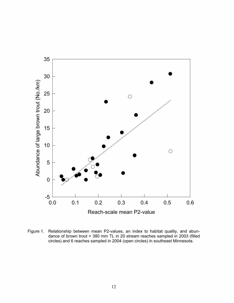
because it explained more deviance than com-parable models with D90. For example, in univariate models, D60 explained 20% of the deviance, whereas D90 only explained 13%. Overhead bank cover, instream rock, and a water depth variable were similarly selected in our P/A model, and help corroborate our find-ings of pool-scale variables influencing large trout. Reach scale Large trout abundance in this study ranged from 0.0–30.7/km, and mean abun-dance was 8.5/km in 2003, 6.1/km in 2004, and 7.2/km for both years. Mean density of large trout in the 20 streams used for model development in this study, was 12.9/ha and ranged from 0.0 to 43.5/ha (Appendix Table A1). Large trout abundance (number/km) was positively related to mean P2-value, dis-charge, mean depth, trout biomass, and water-shed basin area in univariate regressions. However, all variables were significantly cor-related with each other except for mean depth with discharge, trout biomass, and basin area (Table 6), suggesting coefficient estimates would be unstable if other predictor variables besides mean P2-value were added. Mean P2-value alone explained 54% of the variation in large brown trout abundance among the 20 reaches sampled in 2003 plus an additional 6 reaches where sufficient data were collected in 2004 to calculate a reach-scale mean P2-value (y = -3.57 + 51.83x, with σ2 y|x = 41.50, and P < 0.0001; Figure 1). Habitat Quality Classification We ranked the 26 stream reaches from highest to lowest P2-value, and visually inter-preted potential breaks between poor, fair, good and excellent habitat classes (Table 7). Based on these data, we propose the lower bounds for these classes be 0.0, 0.15, 0.30, and 0.50, respectively. Large brown trout abun-dance differed significantly among the four habitat quality classes (Kruskal-Wallis test χ2

= 14.14, df = 3, P = 0.003). The Wilcoxon two-sample test showed that abundance was significantly different between most pairwise comparisons, except fair and excellent habitat quality classes (Z-statistic = 1.39, P = 0.081)

or between good and excellent classes (Z-statistic = 0.50, P = 0.308). This was likely because of small sample size as only two reaches had excellent habitat quality using this method.

Discussion

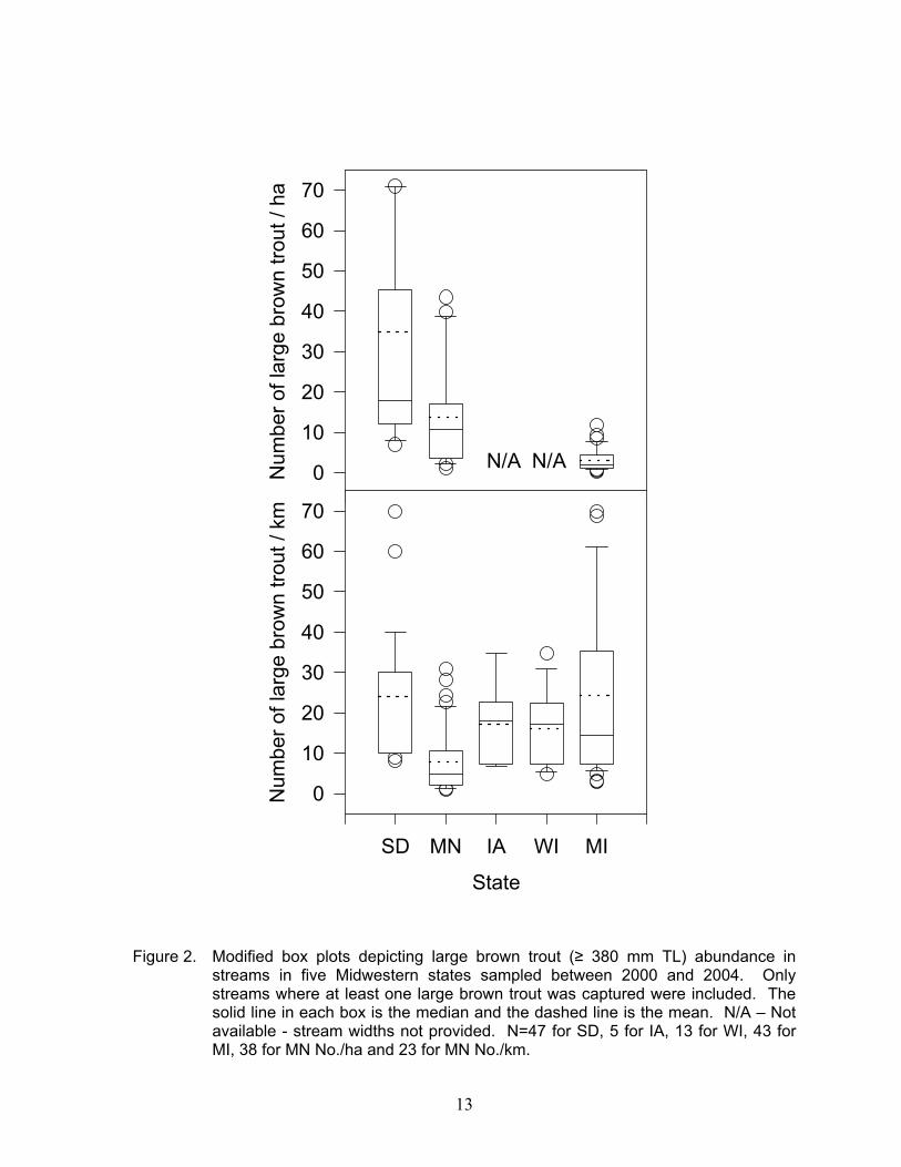
Annear et al. (2004) identified five riverine components as influencing the struc-ture and function of riverine systems: hydrol-ogy, geomorphology / physical habitat, water quality, connectivity / energy sources, and bi-otic interactions. Numerous studies have found relationships between these factors and one or more age- or size-groups of brown trout in streams (e.g., Mesick 1995; Eklöv et al. 1999; Lobón-Cerviá 2004). Results from this study suggest physical habitat and hydrology are important factors limiting large trout abundance in southeast Minnesota streams. In particular, the cover types identified here should be considered as necessary, but not sufficient conditions for a stream to support high densities of large trout. Large trout abundance is generally lower in streams in southeast Minnesota than in other upper Mid-west states (Figure 2). For example, mean number of large brown trout/km was lowest in southeast Minnesota compared with other Midwest states. However, the mean number of large brown trout in southeast Minnesota, expressed as number/ha, was only slightly lower than the mean number/ha in coldwater streams in the Black Hills in South Dakota, but higher than mean number/ha in Michigan (Figure 2). These patterns suggest additional regional features may be important. Our findings confirm several physical habitat features identified by Thorn and Anderson (1993) as being important to large brown trout during summer, but not all of them. Overhead bank cover, instream rocks, and woody debris were significant predictors of large trout presence in a pool in both stud-ies. Presence of deep water, as either D90 in the present study or D60 in the previous study, was also identified. Similarly, our Poisson abundance model selected overhead bank cover, instream rocks, and deeper water, as represented by D60. Pool width was also sig-nificantly associated with large trout abun-dance in pools. Greater pool widths may

11

Table 6. Pearson’s correlation matrix for reach-scale variables significantly related to abundance of large brown trout (No./km) following univariate linear regressions. Data were collected from coldwater streams in southeast Minnesota in 2003 and 2004. Values presented are correlation coefficients (r), with probabilities in paren-theses.

Variable

Large trout abundance

Mean

P2-value

Discharge

Mean depth

Trout biomass (all sizes)

Mean P2-value 0.81 (< 0.001)

Discharge 0.70 (< 0.001)

0.73 (<0.001)

Mean depth 0.52 (0.016)

0.60 (0.005)

0.40 (0.078)

Trout biomass (all sizes)

0.52 (0.018)

0.64 (0.002)

0.56 (0.010)

0.33 (0.150)

Basin area 0.44 (0.047)

0.54 (0.013)

0.65 (0.001)

0.30 (0.185)

0.46 (0.038)

Table 7. Length, number of pools , mean P2-value (a proposed index to habitat quality), and large brown trout (≥ 380

mm TL) abundance (No./km) estimates for 26 stream reaches sampled in southeast Minnesota used to de-velop a reach-scale habitat quality (HQ) classification to guide large trout management. Lower bounds for habitat classes are at mean P2-values 0.0, 0.15, 0.30, and 0.50.

Stream reach

Year

Reach length (km)

No. Pools

Trout abundance

Mean P2-value

H Q Class

Miller Cr.

2003

0.99

15

1.00

0.039

Poor

Daley Cr. – unimproved 2003 0.55 16 0.00 0.047 Poor Watson Cr. – upper 2004 0.85 16 0.00 0.063 Poor Ferguson Cr. 2003 0.32 15 3.14 0.092 Poor Crooked Cr. – North Fork 2003 0.87 13 1.15 0.104 Poor Badger Cr. 2003 0.65 14 1.55 0.117 Poor Big Springs Cr. 2003 0.49 15 0.00 0.146 Poor Wisel Cr. 2003 1.47 18 2.72 0.146 Poor

Lynch Cr. 2004 0.93 16 5.81 0.164 Fair Money Cr. 2003 0.48 15 6.23 0.175 Fair Pine Cr. – unimproved 2004 1.05 14 3.78 0.176 Fair Daley Cr. – improved 2003 0.47 15 2.10 0.189 Fair Thompson Cr. – upper 2004 0.82 17 0.94 0.195 Fair Money Cr. – West Branch 2003 0.45 15 4.40 0.196 Fair Root Rv. – South Branch 2003 0.72 11 1.38 0.208 Fair West Beaver Cr. 2003 0.82 16 9.72 0.223 Fair Etna Cr. 2003 0.53 18 22.64 0.233 Fair Pine Cr. – New Hartford 2003 1.24 14 12.30 0.243 Fair

Spring Valley Cr. 2003 0.87 15 13.74 0.302 Good Root Rv. – South Fork 2003 1.02 14 1.96 0.308 Good Rush Cr. – unimproved 2004 0.53 9 24.16 0.337 Good Bee Cr. 2003 0.75 10 7.07 0.358 Good Main Beaver Cr. – upper 2003 0.75 14 18.80 0.364 Good Rush Cr. – improved 2003 0.89 13 28.22 0.432 Good

Main Beaver Cr. – lower 2003 0.65 8 30.77 0.513 Excellent Pine Cr. – improved 2004 1.00 14 8.24 0.514 Excellent

12

Figure 1. Relationship between mean P2-values, an index to habitat quality, and abun-dance of brown trout > 380 mm TL in 20 stream reaches sampled in 2003 (filled circles) and 6 reaches sampled in 2004 (open circles) in southeast Minnesota.

Reach-scale mean P2-value

0.0 0.1 0.2 0.3 0.4 0.5 0.6

Abu

ndan

ce o

f lar

ge b

row

n tro

ut (N

o./k

m)

-5

0

5

10

15

20

25

30

35

13

Figure 2. Modified box plots depicting large brown trout (≥ 380 mm TL) abundance in streams in five Midwestern states sampled between 2000 and 2004. Only streams where at least one large brown trout was captured were included. The solid line in each box is the median and the dashed line is the mean. N/A – Not available - stream widths not provided. N=47 for SD, 5 for IA, 13 for WI, 43 for MI, 38 for MN No./ha and 23 for MN No./km.

State

SD MN IA WI MI

Num

ber o

f lar

ge b

row

n tro

ut /

ha

0

10

20

30

40

50

60

70

State

SD MN IA WI MI

Num

ber o

f lar

ge b

row

n tro

ut /

km

0

10

20

30

40

50

60

70

N/AN/A

14

indicate a need for greater pool volume in ad-dition to the presence of multiple cover types. Perhaps the presence of multiple cover types promoted presence in a pool by at least one large brown trout, but larger pools, as indi-cated by wider pool widths, promoted pres-ence of multiple large trout. Streambank riprap was not significantly associated with either large trout presence or abundance in pools in the present study. Clearly, shallow pools with little cover do not provide habitat for large brown trout in southeast Minnesota streams. Larger and deeper pools with over-head bank cover, instream rock, and woody debris typically afford protection from preda-tors (Bjornn and Reiser 1991), and may reduce intraspecific competition for space through visual isolation (Sundbaum and Näslund 1998). The pool-scale model of Thorn and Anderson (1993), that predicted P/A of large trout in pools from the presence of five cover variables, was not very good at predicting presence, although it predicted absence well (Table 2). This indicated a need for re-developing the pool-scale model with newer data. Because pools lacking the cover vari-ables identified in Thorn and Anderson (1993) usually did not have large trout present, the presence of these covers was a partial re-quirement, but not the only requirement for large trout presence. If the pools failed to have most of these cover types present, then large trout were usually absent. If, however, the pools had the appropriate cover types, then large trout were present, but only 38% of the time. Other factors may have precluded large trout presence in the other 62% of pools with adequate covers present. The missing physical habitat factors may have been the greater pool depths (i.e., D90) identified in this study, some other unmeasured pool-scale factor, or a factor at a larger spatial scale, such as the reach scale. The low positive predictive value also suggests that the former model did not gener-alize well to new data, possibly because it was overparameterized. Finally, the method Thorn and Anderson (1993) used to select study streams and pools may have inflated the prob-abilities of finding large brown trout and slightly biased their model. Thorn and Ander-son (1993) selected reaches known to have

large brown trout to ensure an adequate sam-ple size for model development. Also, they only measured physical habitat features in an equal number of pools where large trout were present or absent (i.e., as opposed to measur-ing habitat features in all pools large brown trout were absent from). Their approach may have inflated the likelihood of finding large trout overall. Thus, although the pool-scale model of Thorn and Anderson (1993) had some predictive value, we proceeded to de-velop new models based on new data meas-ured across a wider range of stream types that were more representative of conditions in southeast Minnesota. We also included data from all pools sampled for large trout irrespec-tive of whether a large trout was present in each pool or not. Large spatial-scale factors, such as environmental differences among stream reaches, could have influenced large trout abundance and their pool selection, further explaining the low positive predictive value of the Thorn and Anderson (1993) model. A post-hoc analysis, that included a categorical factor for each stream reach sampled in our final pool-scale presence/absence model, indi-cated a significant stream-reach effect on pool-scale presence of large brown trout (log-likelihood ratio test comparing the final multi-ple logistic models with and without the stream-reach factor: -2 log L = 42.773, P < 0.025). This supports the notion that some reach-scale factor(s) were important. Our reach-scale model found large trout abundance to be positively related to mean P2-value, strongly correlated with stream discharge (a hydrology factor), and with watershed area (Table 6). The latter two variables indicate that larger streams have more large brown trout. Stream discharge in late summer was not selected in our final reach-scale model, because it was strongly correlated with the new mean P2-values. This may be because our new P2-value index included D90 and lar-ger streams with greater late summer low flows would likely have a greater frequency of D90 present in pools. Thorn and Anderson (1999) developed a classification scheme for rivers and streams across Minnesota. They speculated that coldwater streams in Class 9 might be some of the best candidates for large

15

brown trout management. Streams in Class 9 were generally the largest coldwater streams with low flow wetted widths exceeding 6 m. Our findings of strong reach-scale positive correlations between large trout abundance and discharge and positive pool-scale associa-tions with pool width, supports their conten-tion. Future analyses should consider use of hierarchical modeling approaches to build and test nested logistic models, to better contrast the relative influences of reach- and pool-scale effects. Such hierarchical modeling ap-proaches include Generalized Linear Models with the Generalized Estimation Equation (GEE), Generalized Linear Mixed Models (GLMM), or Non-Linear Mixed Models (NLINMIX) (Kuss 2002). Abiotic stream features are hierarchi-cally linked, with features at larger spatial scales influencing features at smaller scales (Frissell et al. 1986; Allan 1995; Roth et al. 1996). Such linkages often confound identifi-cation of the most important abiotic variables influencing biotic responses. Widespread col-linearity among many variables at various spa-tial scales has now been detected in several studies of southeast Minnesota streams (Blann 2000, 2004; Dieterman et al. in review; this study, Table 6). Streams with higher dis-charge would be expected to have larger and wider pools with more deep water as reflected in a greater P2-value. Additionally, larger pools may have a higher probability of having a cover type such as woody debris or overhead bank cover present. Thus, large trout may be responding directly to the cover types and greater pool volume, but it is the larger-scale features such as larger basin area and greater discharge that ultimately influence large trout abundance. For example, Thorn and Ander-son (2001b) did not find an increase in large trout abundance in a study of habitat rehabili-tation in Hay Creek, where cover types such as instream rock, riprap, and overhead bank cover were added. They suggested that the lack of increase in large trout abundance may have been due to factors hindering growth, such as water temperature or prey availability. Our results suggest that the lack of an increase may have been due to the smaller stream size of Hay Creek and that riprap was not impor-tant. Future studies of fish and fish habitat

associations should focus more on manipulat-ive studies that isolate the effects of habitat features of interest, so that broad associations identified in previous studies can be verified. Assuming our study reach selection was representative, our method of classifying habitat as poor with mean P2-values < 0.15, fair with values from 0.15 to < 0.30, good with values from 0.30 to < 0.50, and excellent with values ≥ 0.50, met most criteria for a good reach-scale habitat index. This method ac-counted for past stream degradation by classi-fying most reaches as poor (8 reaches) or fair (10 reaches), yet still classified a few reaches as good (6 reaches) or excellent (2 reaches). Large trout abundance differed significantly between poor or fair and good classes, which permits application with the MNDNR (2000) decision-making key. Few excellent-quality reaches likely limited our ability to adequately compare large trout abundance among all four habitat classes. This could be retested if future assessments collect large trout abundance in-formation and classify habitat with this method. Our mean P2-value index to habitat quality may be sensitive to the length of stream sampled, and therefore should not be calculated for reach lengths exceeding those used in its development in this study. We never sampled a stream reach shorter than 0.32 km nor longer than 1.47 km with fewer than 8 pools nor more than 18 pools (Table 7). Larger streams generally had fewer pools per length of reach (personal observation). There-fore, when determining the length of stream to assess for calculation of a mean P2-value, reach lengths may be the best guide for larger streams (i.e., generally watershed basin areas > 5,000 ha and mean widths > 6.0 m), whereas number of pools may be a better criteria to use for smaller streams. A general limitation of studies of as-sociation is that some important variables may not be included in the analysis. Although our results found physical habitat and discharge to be important, associated with presence and abundance of large trout, we did not examine potential influence of water quality, connec-tivity/energy sources, and biotic interactions. Also, some factors may interact and exhibit synergistic effects. For example, Dieterman et

16

al. (2004) suggested that water temperature, a water quality factor, influenced the composi-tion and availability of prey items (i.e., energy sources) that in turn promoted faster growth of brown trout. Previous modeling results showed that large brown trout abundance may be linked to faster growth rates. Dieterman et al. (in review) examined biotic interactions among age 0, 1, and 2 brook Salvelinus fon-tinalis, brown Salmo trutta, and rainbow trout Oncorhynchus mykiss in southeast Minnesota streams. They found trout densities explained at most 15% of the variation in incremental growth, indicating that these biotic interac-tions were of only minor importance in influ-encing growth, and consequently abundance of large brown trout. Other parameters, such as water temperature, that could directly influ-ence large trout P/A and abundance, should be incorporated in future studies, and more ther-mally marginal streams could also be in-cluded. Warmwater stream sampling and angler reports indicate that large brown trout are occasionally captured in streams consid-ered to be too warm for trout for at least a por-tion of each year (MNDNR unpublished data). Finally, angling mortality, another biotic inter-action, is a parameter that could have influ-enced our results and should be examined in future studies. Measurement of angler mortal-ity may necessitate alternative methods of measurement, other than traditional creel sur-veys, because of the low abundance of large brown trout and infrequent creel interviews. For example, Weiss (1999) was unable to es-timate exploitation of brown trout age groups older than age 2 in nine southeast Minnesota streams because of low sample sizes. Our reach-scale abundance model with the new P2-value as a predictor should be further tested. We only collected relevant data to validate our reach-scale abundance model from six reaches in 2004. In the other 15 reaches, we only noted P/A of the 5 cover types (i.e., riprap, woody debris, instream rock, overhead bank cover, and water deeper than 60 cm) identified as important in the original Table 8 of Thorn and Anderson (1993). Thus, we did not have data on P/A of water deeper than 90 cm to validate our reach-model based on the newer mean P2-values (Table 5-this report). However, results from

our pool-scale analyses somewhat corrobo-rated our reach-scale model, because the pri-mary cover components in our reach-scale predictor, P2-value, were derived from pool-scale analyses. This also illustrates the bene-fits of using a multi-scale approach such as ours. Nevertheless, additional data on P/A of overhead bank cover, woody debris, instream rock, and water deeper than 90 cm should be collected in conjunction with trout abundance information to further test our reach-scale model. If catchability of large brown trout was not consistent among our study streams, it could have influenced our results. Conven-tional thinking would suggest that larger streams with greater discharge, depth, and width might reduce large trout catchability. However, our strong positive correlations be-tween large trout abundance and discharge and mean depth (Table 6) indicate that we cap-tured more large trout in larger streams, and casts doubt on the idea of lower catchability in larger streams. If catchability was indeed lower, thean the implication is that our statisti-cal relationships should only be stronger than what we found and the variables we identified should be even more important. In summary, we found large brown trout presence or abundance to be associated with selected physical habitat and hydrology features in pools and reaches of southeast Minnesota streams. Large brown trout are most abundant in the largest streams, as indi-cated by an association with late summer, low-flow discharges. The largest streams may have the best combinations of pool-scale in-stream cover types used by large trout in late summer, and include wide pools, deep water, instream rocks, overhead bank cover, and woody debris. The pool-scale cover types are reflected in our new reach-scale mean P2-value index. Our results should be used to help prioritize streams for large trout man-agement and contribute to an instream habitat management program for large brown trout.

Management Implications

We recommend managers begin pri-oritizing streams for large trout management based on discharge during late summer.

17

Streams with the greatest discharge should have the highest priority. Streams with dis-charge ≥ 0.43 m3/s (the 75th percentile in our dataset) should then be evaluated for habitat quality as measured by the mean P2-value for a representative study reach. Streams with good-excellent habitat quality should be elec-trofished to assess large brown trout abun-dance. Measured large trout abundance should then be compared to expected abun-dance calculated from our reach-scale regres-sion model. If abundance is greater than 25% of the expected value, then the stream should simply be monitored (MNDNR 2000). We suggest that measured abundance values be-tween 25% and 75% of the expected values be considered normal variation. If abundance is lower than the 25th percentile, then other fac-tors such as angler harvest or water chemistry parameters should be investigated. Similarly, values greater than 75% of expected values may suggest influences of factors other than physical habitat. For example, Etna Creek had a measured abundance of large brown trout of 22.6/km that exceeded 75% of the expected value (i.e., 11.4/km) for a stream reach with a mean P2-value of 0.233. Perhaps such high abundance was due to immigration of trout from an adjacent large warmwater stream dur-ing our summer sampling period.

For streams with discharge ≥ 0.43 m3/s and poor-fair habitat quality, we recom-mend instream habitat management. Preva-lence of water deeper than 90 cm, woody debris, instream rocks, and overhead bank cover within pools should be assessed and added as needed. Instream rocks, as boulder clusters, are also an important cover type for large brown trout in winter as shown by Mar-witz et al. (unpublished). For smaller streams with discharge < 0.43 m3/s, large trout management is more complex. These streams are unlikely to have wider and larger pool areas or water deeper than 90 cm. Thus, habitat quality will likely be poor-fair in most instances and managers may simply need to recognize the limited bio-logical potential in these systems for support-ing abundant large trout. Managers may consider increased cooperation with land man-agement agencies, such as the Natural Re-sources Conservation Service, to target

watersheds and implement watershed man-agement approaches to bolster streamflows. Regulatory agencies should also continue to protect late summer baseflows from water withdrawals for municipal, industrial, agricul-tural, or private uses. We recommend that all large trout habitat management, whether in large or small streams of various habitat qual-ity, be considered experimental management and evaluated. Managers should consider collecting information on late summer discharge, large brown trout abundance, and area of overhead bank cover, instream rock, woody debris, rip rap, and water depths exceeding 60, 90, 120, and 150 cm to aid application, evaluation, and refinement of these models. Some variables, such as area of water deeper than 120 or 150 cm, were not adequately evaluated due to ex-treme rarity. Also, continuous variable meas-urements can always be collapsed to P/A, but P/A data cannot be expanded.

The emphasis of these data was on physical habitat, but managers should remain aware of other factors potentially influencing large brown trout, such as water quality and biotic interactions. Biotic interactions with anglers or mammalian and avian predators can result in high mortality for large brown trout (Meyers et al. 1992; Marwitz et al., unpub-lished). Also, large brown trout are able to make extensive long distance movements (Meyers et al. 1992; Young 1994; Bettinger and Bettoli 2004), and connectivity to winter refugium or spawning areas may be extremely important. Such movements could have im-plications in the success of a comprehensive habitat management program. For example, how close do pools with overwintering habitat, in the form of deep water, woody debris, and instream rocks, have to be to pools providing important summer habitat? Can small streams support higher abundances of large brown trout than predicted by our P2-values if con-nected to larger streams? Similar movement studies should be investigated in southeast Minnesota to further our understanding of the importance of habitat quality and juxtaposition to promote greater large trout abundance.

18

References Allan, J. D. 1995. Stream ecology: structure

and function of running waters. Chapman and Hall, New York, New York.

Annear, T., I. Chisholm, H. Beecher, A. Locke, and 12 co-authors. 2004. In-stream flows for riverine resource stewardship, revised edition. Instream Flow Council, Cheyenne, Wyoming.

Bachman, R. A. 1984. Foraging behavior of free-ranging wild and hatchery brown trout in a stream. Transactions of the American Fisheries Society 113:1-32.

Bettinger, J. M., and P. W. Bettoli. 2004. Seasonal movement of brown trout in the Clinch River, Tennessee. North American Journal of Fisheries Man-agement 24:1480-1485.

Bjornn, T. C., and D. W. Reiser. 1991. Habitat requirements of salmonids in streams. Pages 83-138 in W. R. Meehan, edi-tor. Influences of forest and rangeland management on salmonid fishes and their habitats. American Fisheries So-ciety Special Publication 19. Bethesda, Maryland.

Blann, K. L. 2000. Catchment and riparian scale influences on coldwater streams and stream fish in southeastern Minne-sota. Master’s thesis. University of Minnesota, St. Paul.

Blann, K. L. 2004. Landscape-scale analysis of stream fish communities and habitats: lessons from southeastern Minnesota. Doctoral dissertation. University of Minnesota, St. Paul.

Bunnell Jr., D. B., J. J. Isely, K. H. Burrell, and D. H. Van Lear. 1998. Diel movement of brown trout in a south-ern Appalachian river. Transactions of the American Fisheries Society 127:630-636.

Burrell, K. H., J. J. Isely, D. B. Bunnell, Jr., D. H. Van Lear, and C. A. Dolloff. 2000. Seasonal movement of brown trout in a southern Appalachian river. Transac-tions of the American Fisheries Soci-ety 129:1373-1379.

Clapp, D. F., R. D. Clark, Jr., and J. S. Diana. 1990. Range, activity, and habitat of

large, free-ranging brown trout in a Michigan stream. Transactions of the American Fisheries Society 119:1022-1034.

Diana, J. S., J. P. Hudson, and R. D. Clark, Jr. 2004. Movement patterns of large brown trout in the mainstem Au Sable River, Michigan. Transactions of the American Fisheries Society 133:34-44.

Dieterman, D. J., and D. L. Galat. 2004. Large-scale factors associated with sicklefin chub distribution in the Mis-souri and Lower Yellowstone Rivers. Transactions of the American Fisheries Society 133:577-587.

Dieterman, D. J., W.C. Thorn, and C. S. Anderson. 2004. Application of a bioenergetics model for brown trout to evaluate growth in southeast Minnesota streams. Minnesota Department of Natural Resources, Section of Fisheries Investigational Report 513, St. Paul.

Dieterman, D. J., T. D. Marwitz, C. S. Ander-son, W. C. Thorn, and J. L. Weiss. In review. Effects of trout density and other factors upon the growth of brown trout in southeast Minnesota streams. Minnesota Department of Natural Resources, Section of Fisher-ies Investigational Report, St. Paul.

Eklöv, A. G., L. A. Greenberg, C. Brönmark, P. Larsson, and O. Berglund. 1999. Influence of water quality, habitat and species richness on brown trout popu-lations. Journal of Fish Biology 54:33-43.

Frissell, C. A., W. L. Liss, C. E. Warren, and M. D. Hurley. 1986. A hierarchical framework for stream habitat classifi-cation: viewing streams in a watershed context. Environmental Management 10:199-214.

Greenberg, L. A., T. Steinwall, and H. Persson. 2001. Effect of depth and substrate on use of pools by brown trout. Transac-tions of the American Fisheries Soci-ety 130:699-705.

Hatcher, L., and E. J. Stepanski. 1994. A step-by-step approach to using the SAS system for univariate and multivariate statistics. SAS Institute Inc., Cary, North Carolina.

19

Hayes, J. W., and I. G. Jowett. 1994. Micro-habitat models of large drift-feeding brown trout in three New Zealand riv-ers. North American Journal of Fish-eries Management 14:710-725.

Heggenes, J. 1988. Physical habitat selection by brown trout (Salmo trutta) in riverine systems. Nordic Journal of Freshwater Research 64:74-90.

Hosmer, D. W., and S. Lemeshow. 1989. Applied logistic regression. Wiley, New York.

Kuss, O. 2002. How to use SAS® for logistic regression with correlated data. Pro-ceedings of the 27th Annual SAS® Users Group International Conference (SUGI 27), Paper 261-27. Available: www2.sas.com/proceedings/sugi27/p261-27.pdf. (April 2006).

Lobón-Cerviá, J. 2004. Discharge-dependent covariation patterns in the population dynamics of brown trout (Salmo trutta) within a Cantabrian river drain-age. Canadian Journal of Fisheries and Aquatic Sciences 61:1929-1939.

Marwitz, T. D., Thorn, W. C., and C. S. Anderson. (unpublished). Determina-tion of winter habitat of large brown trout in southeast Minnesota streams using radiotelemetry. Minnesota De-partment of Natural Resources, Sec-tion of Fisheries, St. Paul.

McCullagh, P., and J. A. Nelder. 1989. Gen-eralized linear models, 2nd edition. Chapman and Hall, London.

Menard, S. 1995. Applied logistic regression analysis. Sage Publications, Thousand Oaks, California.

Mesick, C. F. 1995. Response of brown trout to streamflow, temperature, and habi-tat restoration in a degraded stream. Rivers 5:75-95.

Meyers, L. S., T. F. Thuemler, and G. W. Kornely. 1992. Seasonal movement of brown trout in northeast Wisconsin. North American Journal of Fisheries Management 12:433-441.

MNDNR (Minnesota Department of Natural Resources). 1978. Minnesota stream survey manual. Minnesota Department of Natural Resources, Section of Fish-eries Special Publication 120, St. Paul.

MNDNR (Minnesota Department of Natural Resources). 2000. Management for large brown trout in southeast Minne-sota streams. Minnesota Department of Natural Resources, Section of Fish-eries Staff Report 57, St. Paul.

Nagelkerke, N. J. D. 1991. A note on a gen-eral definition of the coefficient of de-termination. Biometrika 78:691-692.

Rabeni, C. F. 1992. Habitat evaluation in a watershed context. Pages 56-67 in R. Stroud, editor. Fisheries management and watershed development. American Fisheries Society Symposium 13, Be-thesda, Maryland.

Roth, N. E., J. D. Allan, and D. L. Erickson. 1996. Landscape influences on stream biotic integrity assessed at multiple spatial scales. Landscape Ecology 11:141-156.

SAS Institute Inc. 1999. SAS INSIGHT user’s guide. SAS OnlineDocTM: ver-sion 7-1. SAS Institute Inc., Cary, North Carolina. Available: www.okstate. edu/sas/v7/saspdf/insight/chap17.pdf. (May 2005).

SAS Institute Inc. 2001. SAS/STAT® software: changes and enhancements, release 8.2., SAS Institute Inc., Cary, North Carolina. Available:www.ats.ucla.edu/stat/sas/V8/ gam.pdf.(November 2005).

Sundbaum, K., and I. Näslund. 1998. Effects of woody debris on the growth and behavior of brown trout in experimental stream channels. Canadian Journal of Zoology 76:56-61.

Thorn, W. C., and C. S. Anderson. 1993. Sum-mer habitat requirements of large brown trout in southeast Minnesota streams. Minnesota Department of Natural Resources, Section of Fisheries Investigational Report 428, St. Paul.

Thorn, W. C., C. S. Anderson, W. E. Lorenzen, D. L. Hendrickson, and J. W. Wagner. 1997. A review of trout management in southeast Minnesota streams. North American Journal of Fisheries Man-agement 17:860-872.

Thorn, W. C., and C. S. Anderson. 1999. A provisional classification of Minnesota rivers with associated fish communi-ties. Minnesota Department of Natural

20

Resources, Section of Fisheries Special Publication 153, St. Paul.

Thorn, W. C., and C. S. Anderson. 2001a. Evaluating habitat quality from stream survey variables. Minnesota Depart-ment of Natural Resources, Section of Fisheries Fish Management Report 35, St. Paul.

Thorn, W. C., and C. S. Anderson. 2001b. Comparison of two methods of habitat rehabilitation for brown trout in a southeast Minnesota stream. Minne-sota Department of Natural Resources, Section of Fisheries Investigational Report 488, St. Paul.

Thorn, W. C., C. S. Anderson, and W. E. Lorenzen. In review. Increasing brown trout abundance in southeast Minne-sota streams, 1970-2001.

USDA (United States Department of Agricul-ture). 1991. Revised 1995. State soil geographic (STATSGO) database data use information. National Soil Survey Center, Miscellaneous Publication 1492. Natural Resources Conservation Ser-vice. United States Department of Agriculture, Lincoln, Nebraska.

Weiss, J. L. 1999. Characteristics of the trout fishery on nine southeastern Minnesota streams. Minnesota Department of Natural Resources, Section of Fisheries Completion Report, St. Paul.

White, R. J. 1996. Growth and development of North American stream habitat management for fish. Canadian Journal of Fisheries and Aquatic Sciences 53 (Supplement 1):342-363.

Young, M. K. 1994. Mobility of brown trout in south-central Wyoming streams. Canadian Journal of Zoology 72:2078-2083.

21

Appendix Table A1. Values for biological variables measured to develop a model of large brown trout (LT) abundance (LT/km, LT/ha) in stream reaches in southeast Minnesota.

Stream reach LT/km LT/ha Trout density (#/ha) Trout biomass (kg/ha)

2003 Badger 1.55 5.40 726 99 Beaver, Lower 30.77 43.52 1512 224 Beaver, Upper 18.80 22.53 2115 215 Beaver, West 9.72 14.90 1452 118 Bee 7.07 9.53 1677 160 Big Springs 0.00 0.00 2162 120 Crooked, North Fork 1.15 2.17 809 88 Daley, improved 2.10 7.19 1924 199 Daley, unimproved 0.00 0.00 680 36 Etna 22.64 38.35 2048 72 Ferguson 3.14 10.80 6465 219 Miller 1.00 2.20 181 14 Money 6.23 12.02 20 9 Money, West 4.40 9.87 246 39 Pine (New Hartford) 12.30 15.23 1085 128 Root River, South Branch 1.38 1.19 1977 161 Root River, South Fork 1.96 2.70 1914 110 Rush, improved 28.22 39.91 3565 278 Spring Valley 13.74 17.72 1621 108 Wisel 2.72 3.18 289 56

2004 Lynch 5.81 11.30 1396 64 Pine, improved 8.24 11.58 243 64 Pine, unimproved 3.78 4.59 146 36 Rush, unimproved 24.16 29.23 520 55 Thompson, upper 0.94 2.69 366 60 Watson, upper 0.00 0.00 77 13

22

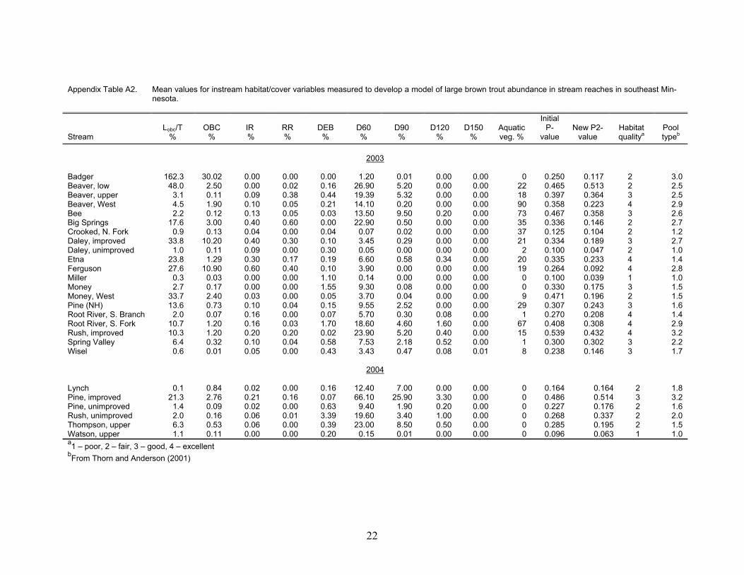
Appendix Table A2. Mean values for instream habitat/cover variables measured to develop a model of large brown trout abundance in stream reaches in southeast Min-nesota.

Stream

Lobc/T

%

OBC

%

IR %

RR %

DEB

%

D60 %

D90 %

D120

%

D150

%

Aquatic veg. %

Initial P-

value

New P2-

value

Habitat qualitya

Pool typeb

2003

Badger

162.3

30.02

0.00

0.00

0.00

1.20

0.01

0.00

0.00

0

0.250

0.117

2

3.0

Beaver, low 48.0 2.50 0.00 0.02 0.16 26.90 5.20 0.00 0.00 22 0.465 0.513 2 2.5 Beaver, upper 3.1 0.11 0.09 0.38 0.44 19.39 5.32 0.00 0.00 18 0.397 0.364 3 2.5 Beaver, West 4.5 1.90 0.10 0.05 0.21 14.10 0.20 0.00 0.00 90 0.358 0.223 4 2.9 Bee 2.2 0.12 0.13 0.05 0.03 13.50 9.50 0.20 0.00 73 0.467 0.358 3 2.6 Big Springs 17.6 3.00 0.40 0.60 0.00 22.90 0.50 0.00 0.00 35 0.336 0.146 2 2.7 Crooked, N. Fork 0.9 0.13 0.04 0.00 0.04 0.07 0.02 0.00 0.00 37 0.125 0.104 2 1.2 Daley, improved 33.8 10.20 0.40 0.30 0.10 3.45 0.29 0.00 0.00 21 0.334 0.189 3 2.7 Daley, unimproved 1.0 0.11 0.09 0.00 0.30 0.05 0.00 0.00 0.00 2 0.100 0.047 2 1.0 Etna 23.8 1.29 0.30 0.17 0.19 6.60 0.58 0.34 0.00 20 0.335 0.233 4 1.4 Ferguson 27.6 10.90 0.60 0.40 0.10 3.90 0.00 0.00 0.00 19 0.264 0.092 4 2.8 Miller 0.3 0.03 0.00 0.00 1.10 0.14 0.00 0.00 0.00 0 0.100 0.039 1 1.0 Money 2.7 0.17 0.00 0.00 1.55 9.30 0.08 0.00 0.00 0 0.330 0.175 3 1.5 Money, West 33.7 2.40 0.03 0.00 0.05 3.70 0.04 0.00 0.00 9 0.471 0.196 2 1.5 Pine (NH) 13.6 0.73 0.10 0.04 0.15 9.55 2.52 0.00 0.00 29 0.307 0.243 3 1.6 Root River, S. Branch 2.0 0.07 0.16 0.00 0.07 5.70 0.30 0.08 0.00 1 0.270 0.208 4 1.4 Root River, S. Fork 10.7 1.20 0.16 0.03 1.70 18.60 4.60 1.60 0.00 67 0.408 0.308 4 2.9 Rush, improved 10.3 1.20 0.20 0.20 0.02 23.90 5.20 0.40 0.00 15 0.539 0.432 4 3.2 Spring Valley 6.4 0.32 0.10 0.04 0.58 7.53 2.18 0.52 0.00 1 0.300 0.302 3 2.2 Wisel 0.6 0.01 0.05 0.00 0.43 3.43 0.47 0.08 0.01 8 0.238 0.146 3 1.7

2004

Lynch

0.1

0.84

0.02

0.00

0.16

12.40

7.00

0.00

0.00

0

0.164

0.164

2

1.8

Pine, improved 21.3 2.76 0.21 0.16 0.07 66.10 25.90 3.30 0.00 0 0.486 0.514 3 3.2 Pine, unimproved 1.4 0.09 0.02 0.00 0.63 9.40 1.90 0.20 0.00 0 0.227 0.176 2 1.6 Rush, unimproved 2.0 0.16 0.06 0.01 3.39 19.60 3.40 1.00 0.00 0 0.268 0.337 2 2.0 Thompson, upper 6.3 0.53 0.06 0.00 0.39 23.00 8.50 0.50 0.00 0 0.285 0.195 2 1.5 Watson, upper 1.1 0.11 0.00 0.00 0.20 0.15 0.01 0.00 0.00 0 0.096 0.063 1 1.0 a1 – poor, 2 – fair, 3 – good, 4 – excellent bFrom Thorn and Anderson (2001)

23

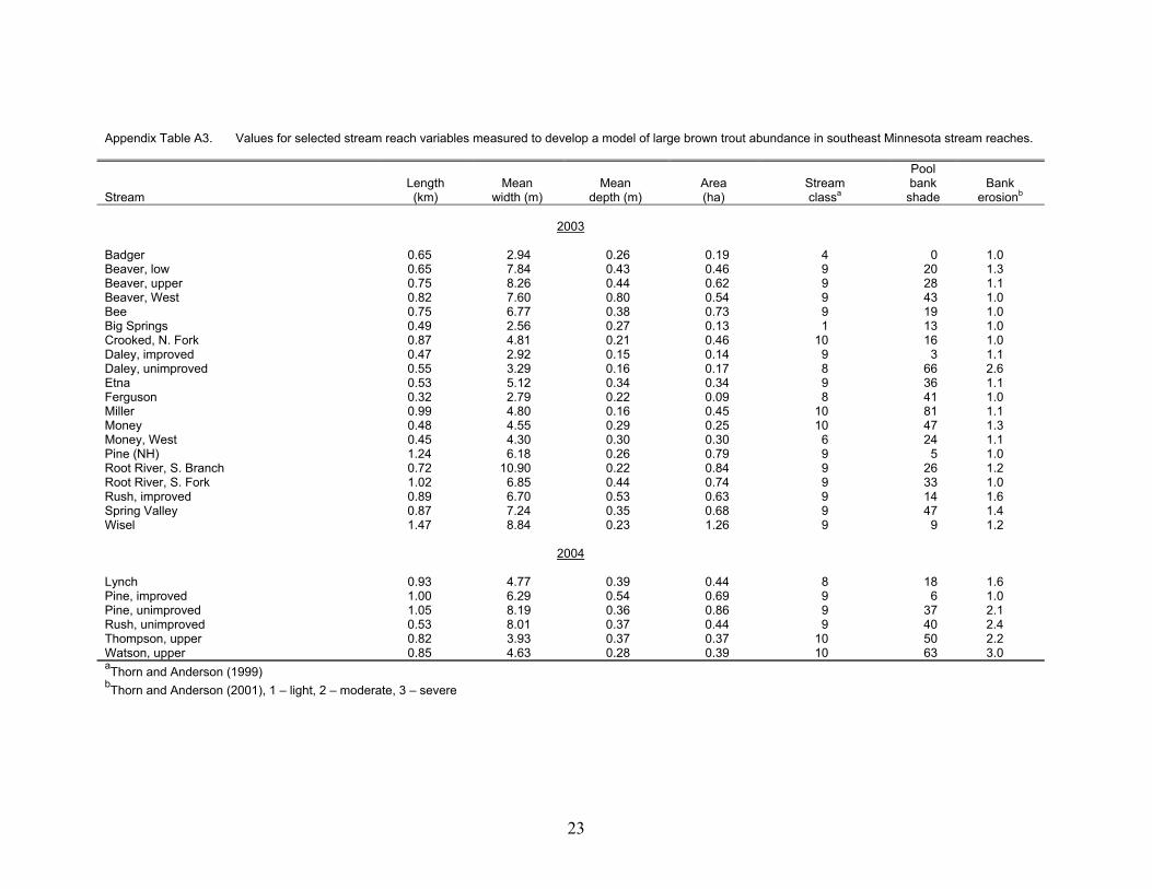
Appendix Table A3. Values for selected stream reach variables measured to develop a model of large brown trout abundance in southeast Minnesota stream reaches. Stream

Length (km)

Mean

width (m)

Mean

depth (m)

Area (ha)

Stream classa

Pool bank

shade

Bank

erosionb

2003

Badger 0.65 2.94 0.26 0.19 4 0 1.0 Beaver, low 0.65 7.84 0.43 0.46 9 20 1.3 Beaver, upper 0.75 8.26 0.44 0.62 9 28 1.1 Beaver, West 0.82 7.60 0.80 0.54 9 43 1.0 Bee 0.75 6.77 0.38 0.73 9 19 1.0 Big Springs 0.49 2.56 0.27 0.13 1 13 1.0 Crooked, N. Fork 0.87 4.81 0.21 0.46 10 16 1.0 Daley, improved 0.47 2.92 0.15 0.14 9 3 1.1 Daley, unimproved 0.55 3.29 0.16 0.17 8 66 2.6 Etna 0.53 5.12 0.34 0.34 9 36 1.1 Ferguson 0.32 2.79 0.22 0.09 8 41 1.0 Miller 0.99 4.80 0.16 0.45 10 81 1.1 Money 0.48 4.55 0.29 0.25 10 47 1.3 Money, West 0.45 4.30 0.30 0.30 6 24 1.1 Pine (NH) 1.24 6.18 0.26 0.79 9 5 1.0 Root River, S. Branch 0.72 10.90 0.22 0.84 9 26 1.2 Root River, S. Fork 1.02 6.85 0.44 0.74 9 33 1.0 Rush, improved 0.89 6.70 0.53 0.63 9 14 1.6 Spring Valley 0.87 7.24 0.35 0.68 9 47 1.4 Wisel 1.47 8.84 0.23 1.26 9 9 1.2

2004

Lynch 0.93 4.77 0.39 0.44 8 18 1.6 Pine, improved 1.00 6.29 0.54 0.69 9 6 1.0 Pine, unimproved 1.05 8.19 0.36 0.86 9 37 2.1 Rush, unimproved 0.53 8.01 0.37 0.44 9 40 2.4 Thompson, upper 0.82 3.93 0.37 0.37 10 50 2.2 Watson, upper 0.85 4.63 0.28 0.39 10 63 3.0 aThorn and Anderson (1999) bThorn and Anderson (2001), 1 – light, 2 – moderate, 3 – severe

24

Appendix Table A4. Stream reach morphology variables measured to develop a model of large brown trout abundance in southeast Minnesota stream reaches. Stream

% Pool

% Riffle

Gradient (m/km)

Sinuosity

Discharge (m3/s)

% Fines

WDa

2003

Badger 100.0 0.0 0.93 1.7 0.197 100.0 11.4 Beaver, low 90.4 9.6 2.00 1.9 0.827 71.3 18.4 Beaver, upper 81.9 18.1 3.53 1.2 0.711 61.7 18.9 Beaver, West 89.7 10.3 3.54 1.6 0.231 33.4 9.5 Bee 85.4 14.6 4.19 1.4 0.216 19.6 7.7 Big Springs 84.2 15.8 5.27 1.6 0.051 70.3 9.6 Crooked, N. Fork 52.3 47.7 5.40 1.2 0.211 46.0 23.4 Daley, improved 77.3 22.8 5.84 1.4 0.073 56.4 19.0 Daley, unimproved 70.1 29.9 3.55 1.4 0.138 72.7 20.2 Etna 89.1 11.9 3.41 1.6 0.069 65.5 15.1 Ferguson 60.4 39.6 11.84 1.5 0.112 35.0 12.6 Miller 87.0 13.0 3.98 1.5 0.203 92.0 30.8 Money 87.8 12.2 4.68 1.6 0.067 67.2 15.9 Money, West 89.5 10.1 3.90 2.7 0.088 79.9 14.6 Pine (NH) 83.1 16.9 3.62 1.7 0.201 46.5 23.4 Root River, S. Branch 77.2 22.8 4.13 2.0 0.222 1.0 49.5 Root River, S. Fork 84.1 15.9 5.14 1.5 0.197 49.0 15.4 Rush, improved 79.2 20.8 3.48 2.2 0.427 55.0 12.6 Spring Valley 81.7 18.3 1.84 2.3 0.293 24.0 21.0 Wisel 81.0 9.0 3.62 1.9 0.195 54.3 38.9

2004

Lynch 85.0 15.0 1.70 2.2 0.117 83.6 10.7 Pine, improved 79.3 20.7 1.59 1.8 0.503 47.0 11.5 Pine, unimproved 82.2 18.8 1.98 1.8 0.503 76.0 22.2 Rush, unimproved 85.4 14.6 3.22 1.7 0.849 74.0 21.2 Thompson, upper 90.6 9.4 2.10 1.4 0.142 78.0 10.4 Watson, upper 80.8 19.2 2.78 2.0 0.161 60.9 16.4 aWidth:Depth ratio

25

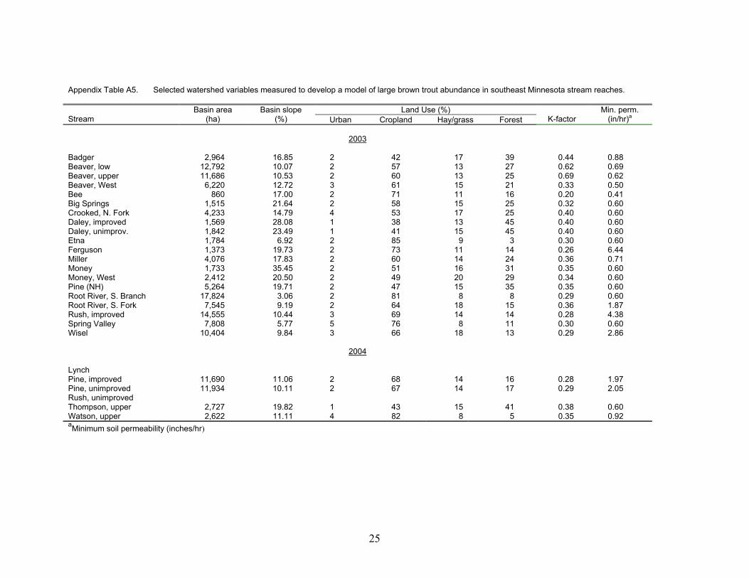
Appendix Table A5. Selected watershed variables measured to develop a model of large brown trout abundance in southeast Minnesota stream reaches.

Land Use (%) Stream

Basin area (ha)

Basin slope (%) Urban Cropland Hay/grass Forest

K-factor

Min. perm. (in/hr)a

2003

Badger 2,964 16.85 2 42 17 39 0.44 0.88 Beaver, low 12,792 10.07 2 57 13 27 0.62 0.69 Beaver, upper 11,686 10.53 2 60 13 25 0.69 0.62 Beaver, West 6,220 12.72 3 61 15 21 0.33 0.50 Bee 860 17.00 2 71 11 16 0.20 0.41 Big Springs 1,515 21.64 2 58 15 25 0.32 0.60 Crooked, N. Fork 4,233 14.79 4 53 17 25 0.40 0.60 Daley, improved 1,569 28.08 1 38 13 45 0.40 0.60 Daley, unimprov. 1,842 23.49 1 41 15 45 0.40 0.60 Etna 1,784 6.92 2 85 9 3 0.30 0.60 Ferguson 1,373 19.73 2 73 11 14 0.26 6.44 Miller 4,076 17.83 2 60 14 24 0.36 0.71 Money 1,733 35.45 2 51 16 31 0.35 0.60 Money, West 2,412 20.50 2 49 20 29 0.34 0.60 Pine (NH) 5,264 19.71 2 47 15 35 0.35 0.60 Root River, S. Branch 17,824 3.06 2 81 8 8 0.29 0.60 Root River, S. Fork 7,545 9.19 2 64 18 15 0.36 1.87 Rush, improved 14,555 10.44 3 69 14 14 0.28 4.38 Spring Valley 7,808 5.77 5 76 8 11 0.30 0.60 Wisel 10,404 9.84 3 66 18 13 0.29 2.86

2004

Lynch Pine, improved 11,690 11.06 2 68 14 16 0.28 1.97 Pine, unimproved 11,934 10.11 2 67 14 17 0.29 2.05 Rush, unimproved Thompson, upper 2,727 19.82 1 43 15 41 0.38 0.60 Watson, upper 2,622 11.11 4 82 8 5 0.35 0.92 aMinimum soil permeability (inches/hr)